Autonomous Excavation of Challenging Terrain using Oscillatory Primitives and Adaptive Impedance Control

Abstract

This paper addresses the challenge of autonomous excavation of challenging terrains, in particular those that are prone to jamming and inter-particle adhesion when tackled by a standard penetrate-drag-scoop motion pattern. Inspired by human excavation strategies, our approach incorporates oscillatory rotation elements – including swivel, twist, and dive motions – to break up compacted, tangled grains and reduce jamming. We also present an adaptive impedance control method, the Reactive Attractor Impedance Controller (RAIC), that adapts a motion trajectory to unexpected forces during loading in a manner that tracks a trajectory closely when loads are low, but avoids excessive loads when significant resistance is met. Our method is evaluated on four terrains using a robotic arm, demonstrating improved excavation performance across multiple metrics, including volume scooped, protective stop rate, and trajectory completion percentage.

I INTRODUCTION

Autonomous excavation — which refers to the navigation, loading, and planning of removing or depositing materials without the assistance of a human driver — is a promising frontier of robotics [1]. Excavation is an economically important activity for constructing roadways, foundations for buildings, and earth structures in forward military bases, as well as mining and waste handling operations, and automated excavation has been studied for decades since the pioneering work of Singh [2] in relation to planning [3], perception [4], and control [5]. This paper focuses on excavation trajectory planning and execution. Whereas standard excavation motions perform well in some terrains, particularly in homogeneous, fine-grained terrains and non-compacted soils, they may fail to yield a sufficient volume or excavation profile in more complex terrains [6]. In particular, tool-material interactions experienced during an excavation loading cycle may be unpredictable due to jamming phenomena in rocky materials and variability in terrain composition, such as large embedded rocks and tree roots hidden beneath a soil surface [5, 7, 8]. Moreover, unusual inter-particle interactions like adhesion and snagging occur when particle shapes are highly irregular, such as those observed in organic terrains like mulch, and can significantly reduce excavated volumes. Although human operators observe terrain response and adjust their excavation strategy appropriately for a given terrain, prior work has not adequately addressed these issues in the automated case.

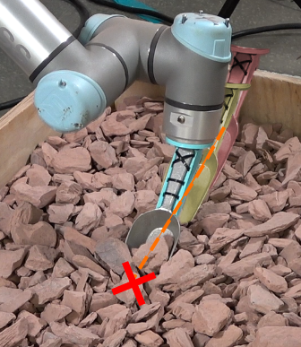
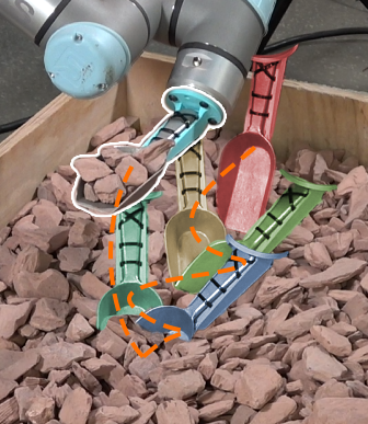
Figure 1: Strobe-effect visualization of a robot excavating large-grained slate. Motion of the scoop is illustrated via tinting progressing from red to blue hue. Left: standard Penetrate-Drag-Scoop (PDS) motion with impedance control fails due to jamming forces triggering a protective stop (red X). Right: using our “swivel” primitive and Reactive Attractor Impedance Controller (RAIC), the robot breaks through jammed particles and excavates a large volume (outlined in white). Trajectory of the scoop is illustrated as an orange curve.

The majority of prior autonomous excavation work uses a predefined trajectory class: penetrate-drag-scoop (or penetrate-drag-curl), in which an excavator bucket first penetrates the terrain with its leading edge, the bucket is dragged through the terrain, and the bucket is rotated to lift the material away from the terrain [9]. The penetration angle, depth, and drag length can be adjusted for a given terrain. Inspired by observations of human adjustments of excavation strategies in such terrains, we introduce a class of variations to the basic primitive that uses oscillations to break up grains to reduce the rate of jamming and encourage disentangling between irregular grains. We empirically examine the effect of sinusoidal rotation perturbations along different axes, frequencies, and amplitudes as the scoop penetrates the terrain.

Moreover, although impedance control [10] is a common strategy to introduce compliance in excavation [11, 12], standard methods of impedance control are still prone to jamming and exceeding safe force limits in challenging terrain. We introduce a novel adaptive method for trajectory tracking control, Reactive Attractor Impedance Controller (RAIC), that alleviates the jamming problem found in the loading cycle by adapting the progress of the impedance control attractor along the tracked path according to the experienced resistance. At low resistance the attractor moves at full speed, and slows if resistance is high. Our experiments evaluate our approach in a variety of terrains, demonstrating that the combination of oscillatory primitives and adaptive impedance significantly increase excavated volumes and reduce protective stop rates in challenging terrain. Moreover, the RAIC controller can even adapt to hidden immovable obstacles embedded in the terrain.

II Related Work

II-A Excavation

Automating excavation is a long-standing and ongoing effort towards creating more efficient construction worksites [13, 14]. Previous studies have shown that autonomous excavation can increase fuel efficiency [15], decrease load time [16, 17], and replace human workers in dangerous environments such as underground-mine excavation [18]. Planning, perception, control, and learning are the key ingredients of autonomous excavation systems [2]. Although much interesting work addresses high-level perception and decision making for orchestrating navigation and excavation locations [3, 4], we focus in this paper on lower-level problems of trajectory planning and control once an excavation location, depth, and drag length have been chosen.

II-B Excavator Trajectory Planning

Yao et al. [15] use a trajectory optimization method to fill a Load-Haul-Dump machine bucket to a desired fill factor while minimizing fuel usage and constraining the optimization to safe torque limits. While this trajectory optimization method proved to create more fuel efficient trajectories, the work assumes the soil is homogeneous and requires prior knowledge on the composition of the material. Fragmented rock has been identified as a challenge for standard excavation approaches [19, 20, 5]. Vision-based learning techniques [19, 20] have been applied to identify areas between rocks in which the bucket edge should begin excavating. However, these learning approaches focused on finding location and shape parameters for the standard penetrate-drag-scoop primitive rather than maneuvering the scoop.

II-C Excavation Control

Open-loop excavation control can be dangerous during jamming or when encountering unexpected obstacles, as high forces can cause damage to actuators and or tip an excavator over. Impedance control [11, 10, 21] and admittance control [5, 22] have been proposed to modify the controls and comply to unexpected terrain resistance. Here, the robot tracks the end effector toward an attractor pose, but also responds to measured forces using a mass-damper simulation [23]. Controller parameters can be learned iteratively by observing excavated fill weight and adjusting parameters to help obtain a desired weight for novel terrain materials [22]. Although standard impedance / admittance control achieves compliance to unexpected forces, it can still encounter large forces when the distance between the current and target pose grows large due to substantial obstructions. Azulay et. al. recently proposed an end-to-end deep reinforcement learning model that directly controls the velocity, bucket tilt and lift of an LHD machine [24]. Egli et al. [25] also propose an RL model that directly drives joint velocities of a wheeled loader. The RL policy is rewarded for quick and filling scoops and negatively rewarded for erratic movements and self collisions. Although this study provides promising results for RL controlled excavation, the work is mostly limited to soft, homogeneous soils. Our proposed controller is an adaptation of impedance control tailored for severe cases of jamming, and it requires far less tuning than RL-based methods.

III Methodology

Motivated by observations of human strategies for excavating challenging terrains, we present parameterized scooping primitives that enhance the standard penetrate-drag-scoop (PDS) trajectory, and the Reactive Attractor Impedance Controller (RAIC) which enhances standard impedance control.

III-A Parameterized Scooping Primitive

The penetrate-drag-scoop (PDS) trajectory, illustrated in Fig. 2, is a three-phase loading cycle widely employed by earth-moving vehicles such as backhoes, wheeled loaders, and excavators. This trajectory begins at a point p and moves in a plane with $x$ direction aligned to a heading $\theta_{\text{base}}$ and $y$ direction vertical. The scoop will also pitch in a prescribed manner about the axis perpendicular to this plane. The cycle begins with a penetration phase, where the end-effector enters the target material at an attack angle $\alpha$, reaching a depth d. Subsequently, in the dragging phase, the scoop maintains its initial attack angle while being dragged linearly for a distance l. The final scooping phase involves rotating the scoop to a closing angle $\beta$, followed by a vertical ascent to height h, thus extracting the scooped material. The trajectory can be described as:

$$\mathbf{T}_{\text{PDS}}(t)=\begin{cases}\mathbf{T}_{\text{penetrate}}(t),&0\leq t<t_{1}\\ \mathbf{T}_{\text{drag}}(t),&t_{1}\leq t<t_{2}\\ \mathbf{T}_{\text{scoop}}(t),&t_{2}\leq t\leq t_{3}\end{cases}$$ (1)

where $\mathbf{T}(t)\in SE(3)$ represents the scoop tip pose in the world frame at time $t$, and $t_{1}$, $t_{2}$, and $t_{3}$ are the transition times between phases.

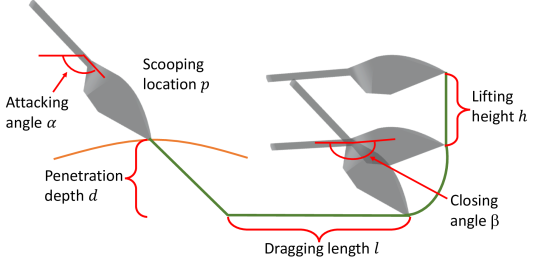
Figure 2: Illustration of the PDS trajectory.

Although PDS is effective at scooping fine-grained granular media, it suffers in terrains where penetration is difficult due to jamming and in terrains with high inter-particle friction forces. To help alleviate these inter-particle forces, we extend the standard PDS trajectory with three novel scooping primitives inspired by motions humans use when scooping materials: the swivel, the twist, and the dive. These primitives introduce variable frequency and amplitude perturbations designed to improve performance in terrains prone to jamming or containing irregular materials.

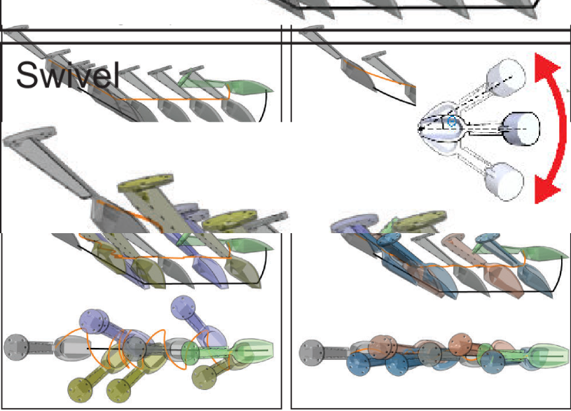
Figure 3: Illustration of our proposed primitives. Bottom row shows side and t op-down views of oscillatory trajectories. Scoop tint indicates magnitude of roll (cyan - orange), yaw (blue - yellow), and pitch (green).

III-A1 Swivel Primitive

Swiveling introduces an oscillatory rotation about the scoop’s tip, aiding in breaking inter-particle friction and disrupting jammed particles when the scoop tip encounters resistance. It is defined by amplitude $A_{\text{swivel}}$ and frequency $f_{\text{swivel}}$ with yaw defined by:

$$\theta_{\text{swivel}}(t)=A_{\text{swivel}}\sin(2\pi f_{\text{swivel}}t).$$ (2)

This yaw value is added to the base yaw $\theta_{\text{base}}$ from the beginning of the penetration phase to the end of the dragging phase. During the scoop phase we return the yaw to $\theta_{\text{base}}$.

III-A2 Twist Primitive

Twisting introduces an oscillatory rotation about the scoop’s longitudinal axis, and helps disentangle particles outside of the scoop from dragging out particles inside of the scoop, which is particularly effective in materials with high inter-particle adhesion. The roll angle is parameterized by amplitude $A_{\text{twist}}$ and frequency $f_{\text{twist}}$ as:

$$\phi_{\text{twist}}(t)=A_{\text{twist}}\sin(2\pi f_{\text{twist}}t)$$ (3)

Like the swivel, twisting is only active from the beginning of the penetration phase through the end of the drag phase. During the scoop phase the roll is returned back to 0.

III-A3 Dive Primitive

Diving modifies the translation and pitch of the penetration and drag phases of the PDS trajectory, creating a smooth, continuous curve. It is parameterized by a dive curve factor $s\in[0,1]$, where $s=0$ corresponds to the original PDS trajectory and $s=1$ generates a fully smooth curve. The dive trajectory modifies the drag phase such that the drag phase becomes replaces by this smoothed trajectory as $s$ increases to one. We define $\mathbf{p}_{\text{smoothed}}(u)$ as a quadratic Bézier curve using the penetration point, the original starting pose of dragging phase $p_{dragstart}$ and drag length $s\cdot l$ from $p_{dragstart}$ as control points. Given the parameter $s$, the trajectory of the end effector is given by:

$$\mathbf{p}_{\text{dive}}(u)=(1-s)\mathbf{p}_{\text{drag}}(u)+s\mathbf{p}_{\text{smoothed}}(u)$$ (4)

where $\mathbf{p}_{\text{drag}}$ is the translation defined by the original PDS $\mathbf{T}_{\text{drag}}$ trajectory, and $u$ is the normalized trajectory parameter. To smooth out and replace the drag phase as $s$ increases, we linearly shrink the drag phase by $(1-s)*l$ such that at $s=1$ the drag phase is fully replaced by $p_{\text{smoothed}}$ with $p_{smoothed}$ using control points $p$, $p_{dragstart}$, and drag length $l$ from $p_{dragstart}$. In addition to smoothing translation, the dive curve modifies the pitch of the scoop to keep the scoop edge traveling tangent to the curve. The pitch at time t is defined as follows:

$$\text{pitch}(t)=tan^{-1}(p^{\prime}_{z}/\sqrt{\Delta p_{x}^{\prime 2}+p_{y}^{\prime 2}})$$ (5)

This modification facilitates more effective media penetration and encourages particle ingress into the scoop during the loading cycle.

We found that this primitive is most useful when paired with the swivel or twist motions as keeping the scoop tangent to its motion allows for the oscillatory movements to more easily cut through the materials.

These primitives can be applied individually or in combination, allowing for adaptive scooping strategies tailored to specific terrain characteristics. Given a set of desired parameters $(A_{\text{swivel}},f_{\text{swivel}},A_{\text{twist}},f_{\text{twist}},s)$, the three primitives are combined to provide the pose trajectory for the scoop as follows. First, we convert our roll, pitch and yaw into a combined rotation matrix, defined as:

$$R_{\text{prim}}(t)=R_{z}(\theta_{\text{base}}+\theta_{\text{swivel}}(t))\cdot R_{y}(\text{pitch}(t))\cdot R_{x}(\phi_{\text{twist}}(t))$$

where $R_{x}$, $R_{y}$, and $R_{z}$ are rotation matrices about the elementary axes. The translation is defined by $\mathbf{p}_{\text{dive}}$ (4), which is identical to the PDS translation trajectory if $s=0$. In the scoop phase, the pitch linearly interpolates from pitch($t_{2}$) to closing angle $\beta$ to finish the scooping trajectory, and the swivel and twist are interpolated to 0 to keep the scoop level upon termination.

III-B Reactive Attractor Impedance Controller

Our RAIC controller is a modification of a standard impedance controller that avoids applying excessive forces while following a target trajectory. RAIC behaves exactly like an impedance controller does in zero-to-little resistance materials, but limits how far the attractor moves away from the end effector when it experiences a lack of progression in medium-to-high resistance materials.

Standard impedance control attracts the current end-effector pose $\mathbf{T}$ to the planned pose $\mathbf{T}^{\text{plan}}$ via a simulating a spring-damper system. Instead, RAIC evolves an attractor pose $\mathbf{T}^{\text{att}}$ to move along the planned trajectory when loads are low, but allows deviations when they are high, which avoids approaching the robot’s force / torque limits. Moreover, our control scheme allows the attractor point to become “unstuck” if the plan pulls it in a direction that may relieve currently accumulated load.

More specifically, we define $\mathbf{T}_{t}\in SE(3)$ as the current end-effector pose at time $t$, and $\mathbf{T}^{\text{plan}}_{t}$ the planned pose, and attractor pose as $\mathbf{T}_{0}^{\text{att}}$. Let $\mathbf{f}=[f_{x},f_{y},f_{z},\tau_{x},\tau_{y},\tau_{z}]^{\top}\in\mathbb{R}^{6}$ be the vector of measured forces and torques from a force/torque sensor. We also define two elementary operators. The first computes the difference vector between poses as

$$d(\mathbf{T}^{\prime},\mathbf{T})=[\omega(\mathbf{R}^{\prime})^{-1}\mathbf{R},\mathbf{p}^{\prime}-\mathbf{p}]\in\mathbb{R}^{6}$$ (6)

where the notation $\mathbf{R}\in SO(3)$ and $\mathbf{p}\in\mathbb{R}^{3}$ split a pose into its rotation and position components, and $\omega(R)$ gives the rotational displacements of $R$ about the $x$, $y$, and $z$ axes. Conversely, the integration operator $int(\mathbf{T},\psi)$ to apply a difference vector $\psi$ to a pose. This operator acts as an inverse of $d$, such that $\mathbf{T}^{\prime}=int(\mathbf{T},d(\mathbf{T}^{\prime},\mathbf{T}))$.

The attractor begins at $\mathbf{T}_{0}^{\text{att}}=\mathbf{T}_{0}$ and evolves along $\mathbf{T}^{\text{plan}}$ according to a feedforward and feedback component. Specifically, we compute the difference in the planned pose

$$\mathbf{d}=d(\mathbf{T}^{\text{plan}}_{t+1},\mathbf{T}^{\text{plan}}_{t})$$ (7)

and the difference from the planned pose to the attractor position

$$\mathbf{e}=d(\mathbf{T}^{\text{plan}}_{t},\mathbf{T}^{\text{att}}_{t}).$$ (8)

The attractor update is given by a damped proportional control with feedforward and feedback terms:

$$\mathbf{T}^{\text{att}}_{t+1}=int(\mathbf{T}^{\text{att}}_{t},D(\mathbf{f},\mathbf{e})\mathbf{d}^{\prime}+F(\mathbf{f},\mathbf{e})\mathbf{e}).$$ (9)

Here, $\mathbf{d}^{\prime}$ is a small modification to $\mathbf{d}$ that discards feedforward directions that close the gap between the plan and the attractor:

$$d_{i}=d_{i}\cdot\min(1+sign(d_{i}\cdot e_{i}),1).$$

The gains $D$ and $F$ are defined such that $D=I$ and $E=I$ when resistive forces are low, and they are close to 0 when resistive forces are high and the planned differences are pointing opposite to the felt forces.

Specifically, we define a damping function $\phi_{i}:\mathbb{R}\rightarrow[0,1]$ for each axis $i$:

$$\phi_{i}(f_{i})=\text{clip}(1-s_{i}|f_{i}-c_{i}|,0,1)$$ (10)

where $s_{i}>0$ is a scaling factor and $c_{i}$ is a cutoff value for axis $i$. $\phi_{i}$ creates a piecewise linear damping effect that begins at 1, starts decreasing linearly at $c_{i}$, and saturates at 0.

We also define an “exit” damping function $\varphi_{i}\rightarrow[0,1]$ for each axis $i$:

$$\varphi_{i}(f_{i},e_{i})=\max(0,\tanh(f_{i}\cdot e_{i}))$$

Where $e_{i}$ is the corresponding element of $\mathbf{e}$. $\varphi_{i}$ is 0 when the direction from the attractor to the plan opposes the direction of sensed forces, and rises to 1 when they are in the same direction.

Overall, the feedforward damping function is

$$\lambda_{i}(f_{i},e_{i})=\max(\phi_{i}(f_{i}),\varphi_{i}(f_{i},e_{i}))$$

and the damping matrix $\mathbf{D}\in\mathbb{R}^{6\times 6}$ is

$$\mathbf{D}=\text{diag}(\lambda_{1}(f_{1},e_{1}),\ldots,\lambda_{6}(f_{6},e_{6})).$$ (11)

For the feedback gain, we use a similar piecewise linear damping. Governed by feedback scales $s^{\text{fb}}_{i}$ and cutoffs $c^{\text{fb}}_{i}$, we define:

$$\phi^{fb}_{i}(f_{i})=\text{clip}(1-s^{fb}_{i}|f_{i}-c^{fb}_{i}|,0,1)$$

and

$$\lambda^{fb}_{i}(f_{i},e_{i})=\max(\phi^{fb}_{i}(f_{i}),\varphi_{i}(f_{i},e_{i}))$$

giving the feedback damping matrix

$$\mathbf{F}=\text{diag}(\lambda^{fb}_{1}(f_{1},e_{1}),\ldots,\lambda^{fb}_{6}(f_{6},e_{6}))$$ (12)

The attractor is used as the target for a standard impedance controller. A spring-damper system is simulated as follows. First, given the difference from the current pose to the attractor,

$$\mathbf{e}^{spring}=d(\mathbf{T}^{\text{att}}_{t},\mathbf{T}_{t}),$$

We simulate a spring-damper with $\mathbf{f}$ as an external force:

$$M\ddot{x}+B\dot{\mathbf{e}}^{spring}+K\mathbf{e}^{spring}=\mathbf{f}.$$ (13)

Here $M$ is the inertia matrix, which we set to an identity, $B$ is the damping matrix, and $K$ is the spring stiffness. We set $B$ and $K$ to diagonal matrices with isotropic behavior in rotation and in translation. Solving for the acceleration $\ddot{x}$, we then double integrate $\ddot{x}$ to find a difference $\Delta x$, which is then added to the end-effector pose:

$$\mathbf{T}_{t+1}=int(\mathbf{T}_{t},\Delta x).$$

IV Experiments and Results

IV-A Setup Overview

Our experimental testbed consists of a Universal Robots UR5e robot arm equipped with a metallic scoop as its end effector. We use the built-in force-torque sensing of UR5e for implementing impedance control as well as RAIC. As a cobot, the UR5e implements a notion of a P-stop (protective stop) that detects potential damage and halts motion. We use P-stop rate as a proxy for a high-force event in which a robot or construction machinery could experience irreversible damage.

An Intel RealSense L515 RGB-D camera mounted above the workspace is used to estimate the volume of excavated material. Excavation occurs in a filled wooden box measuring 0.9 m x 0.6 m x 0.2 m and placed so that the robot is unlikely to reach the end of its workspace. We selected four terrain materials with a diverse set of physical properties: Pebbles, Gravel, Slate, and Mulch. Pebbles, with particles 3-8 mm in diameter, introduces moderate challenges in terms of inter-particle friction and potential jamming. Mulch present unique difficulties due to their irregular shape and tendency to interlock, testing our system’s ability to handle materials with high inter-particle friction and potential for entanglement. Gravel and Slate, approximately 2-5 cm in size, represent the most challenging terrain, prone to severe jamming and requiring substantial force to manipulate.

Pebbles	Gravel	Slate	Mulch

TABLE I: Materials in test terrains, with U.S. quarter coin shown for scale.

IV-B Controller Parameter Tuning

Our methodology for choosing the parameters of our impedance controller and RAIC are as follows. Finding that a stiff controller performs better in rocky terrains than more compliant settings, we chose base impedance controller parameters sufficiently large to penetrate the slate material using the PDS trajectory. We slowly increased K values until penetration was possible, which occurred at 750 N/m for linear stiffness values and 80 Nm/rad for rotational stiffness. Next we tuned damping values until the scoop’s oscillations when hitting hard terrain were minimal. We found these damping values to be 330 Ns/m for linear damping and 12 Nms/rad.

Next, we set the parameters of the RAIC controller as a fixed function of the force and torque values that trigger protective stops in the UR5 arm. We did this by firmly pushing on the tip of the end-effector until the arm triggered a protective stop and logging the magnitude of the force and torque values. We found these to be $F_{\text{max}}$ = 60 N and $T_{\text{max}}$ = 10 Nm respectively. We then set the cutoffs $c_{i}$ to be 25% of their respective maxes and set the scaling values $s_{i}$ to be 1/(50%) of their respective maxes. So, RAIC decouples the attractor point from the planned pose when 25%-75% of the max loads are encountered. For the feedback cutoffs, we set the cutoffs $c^{fb}_{i}$ to be 0 and set their scaling values $s^{fb}_{i}$ to be 1/(25%) of their respective maxes. This is so that the attractor pose is pulled to the plan only when loads are low.

IV-C Effects of Primitive Parameters

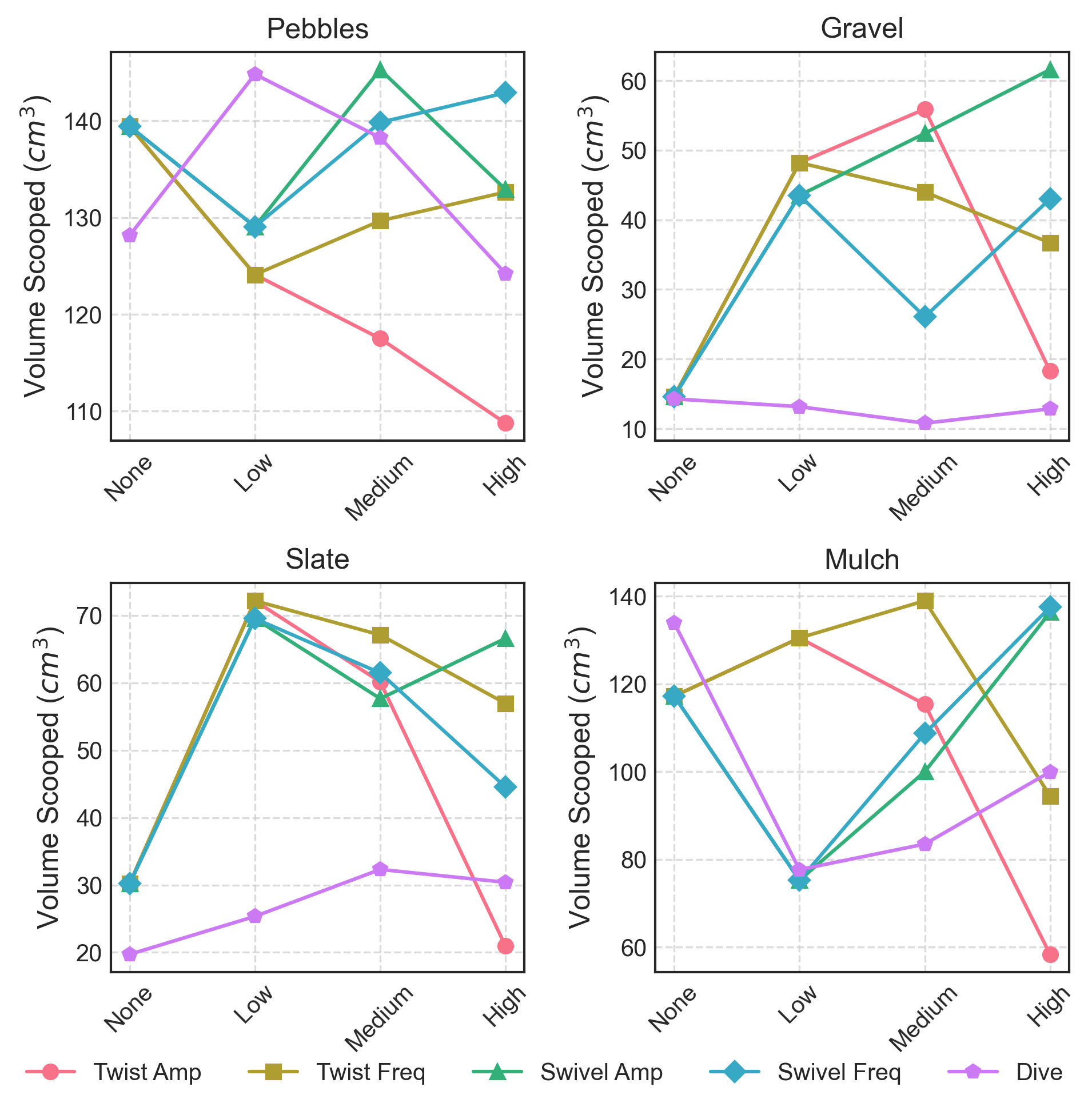
Figure 4: Parameter exploration showing how primitive parameter settings are related to excavated volume. Dive sweep = None is equivalent to the standard penetrate-drag-scoop trajectory.

Next, we explore the effects of parameter settings on our proposed primitive trajectories. On each of our four terrains, we performed parameter sweeps along the five proposed parameters: swivel amplitude/frequency, the twist amplitude/frequency, and the dive curve. Each scoop maintains static values for depth of .07 m, drag length of .25m, and attack angle of 5$\pi$/6 radians.

For each setting we performed 6 (12 on slate for verification purposes) scoops and measured the excavated volume, counting P-stop events as 0. For each parameter, we swept through the primitive at zero, Low, Medium, and High setting. The swivel amplitude sweep considers $A_{\text{swivel}}$ at $\pi$/16, $\pi$/8, and 3$\pi$/16 rad while keeping $f_{\text{swivel}}$ at the Low frequency ($\pi$ rad/sec). The twist amplitude sweep consideres $A_{\text{twist}}$ at $\pi$/12, $\pi$/6 and $\pi$/4 rad respectively while keeping $f_{\text{twist}}$ at the same Low frequency. Both swivel and twist frequency parameter sweeps vary $f_{\cdot}$ amongst $\pi$, 2$\pi$, and 4$\pi$ rad/sec while maintaining Low amplitude. For the dive curve, $s$ is varied between 0.33, 0.66, and 1.0. All other parameters are set to 0. Fig. 4 shows the results from these sweeps.

We found that oscillatory movements during the loading cycle improved the average volume scooped in the difficult Slate and Gravel terrains, while showing little improvement in easier terrains such as Pebbles. For Gravel and Slate, we found that medium-high settings for swivel helped break up frictional forces that caused particles to jam. We also found that twisting at small amplitudes but low-medium frequencies helped improve volume scooped in materials with larger particle sizes. However, twisting at higher amplitudes in lost some material due the roll of the scoop becoming too aggressive, spilling material from the sides.

As for the dive curve, we found that although maintaining a pitch tangential to the trajectory improved performance when combined with a swivel or twist motion, the value of dive curve itself did not affect the results much. In Slate, we can see a minor improvement when we varied $s$ from 0 to 1, however in the other materials we saw an unsubstantial difference in volume scooped between the different values.

IV-D Ablation studies

We next perform ablation studies to examine the effects of our primitives and the RAIC controller (Tab. II). The four experimental conditions use were on the impedance controller using the PDS trajectory, impedance controller plus our scooping primitive trajectory, our RAIC controller using the PDS controller and our RAIC controller using our scooping primitive trajectory. For the scooping primitive trajectory, we used the best parameters described in our parameter tuning section. Both the impedance controller and RAIC controller use the tuned parameters found in our parameter tuning experiments of 750 N/m linear stiffness, 80 Nm/rad rotational stiffness, 320 Ns/m linear damping and 12 Nms/rad rotational damping. In each study we perform 12 (30 on slate for verification purposes) scoops per terrain in batches of 2 pre-defined penetration points. The scoop parameters used in these experiments are .07 m depth, .25 m drag length, and attack angle of 5$\pi$/6 radians.

We computed 3 metrics: volume scooped, P-stop rate, and completion percentage. Completion percentage is defined as the percentage of the trajectory executed before a P-stop occurred. In the easy Pebbles terrain, standard methods work adeuqately well. However, the RAIC controller helps prevent protective stops in harder terrains, especially Gravel and Slate. In these terrains, P-stops were frequently triggered, often during the penetration phase or early drag phase as indicated by the low completion percentages. Behavior in Mulch was also slightly improved using RAIC, although it is not clear whether these results are statistically significant due to the high variance in scooped volumes.

Beyond RAIC, our scooping primitives both helped reduce the number of P-stops as well as increased average scoop volume in most cases. In Gravel and Slate, oscillations broke the friction forces that caused the particles to jam as well as displaced particles that were interlocked with one another, increasing volume and reducing P-stop rate to nearly 0%.

IV-E Hidden Obstacle Compliance

Finally, we performed two qualitative experiments to show how the RAIC controller complies with hidden obstacles, as an excavator can often encounter tangled roots, large boulders, or other unseen obstructions in the terrain.

The first experiment embeds a fixed slope into gravel. For this experiment, we set the depth to be .06 m, drag length of .35 m, and an attack angle of 5$\pi$/6 radians. Primitive settings include High $A_{\text{swivel}}$, Low $f_{\text{swivel}}$, and a dive curve $s=0.5$. Compared to a standard impedance controller, RAIC is able to comply to the slope and successfully excavate material (Fig. 5, left).

The second experiment embeds a large stone into soft soil. We created an indentation in the terrain, placed a large rock in the center of it, and refilled the soil to cover the rock, lightly compacting it. The primitive parameters are unchanged from the ablation studies, using the dive primitive at dive curve $s=0.5$. Compared to standard impedance control, which jams against the rock, RAIC is able to both slow down the trajectory and scoop underneath the rock, leading to the successful completion of the trajectory.(Fig. 5, right)

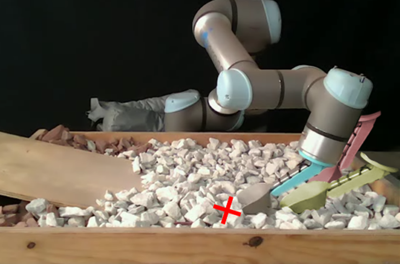
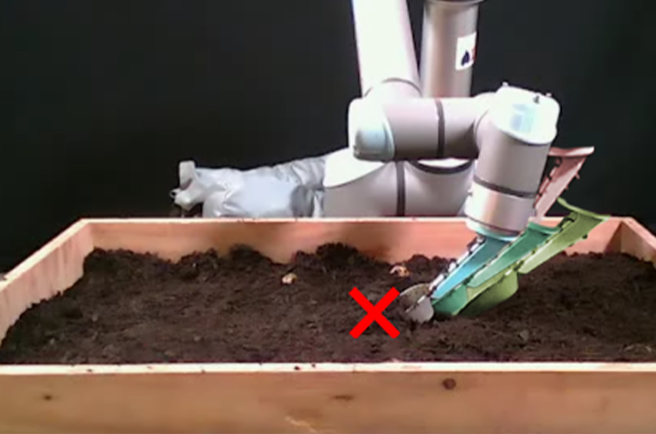
Figure 5: Testing on hidden obstacles, showing movement via strobe-effect. Left: a rigid slope is embedded in gravel. Right: a large rock embedded in soil. Top row: a standard impedance controller is unable to comply to these obstacles when jamming is encountered, triggering a protective stop. Bottom row: the RAIC controller successfully adapts to these obstacles.

TABLE II: Performance comparison of control methods across test terrains. Volume averages and standard deviations are presented. Bold value indicates best mean on a given terrain

Method	Material	Volume (cm³)	P-stop rate (%)	Completion %
Impedance + PDS	Pebbles	134.5 $\pm$ 24.4	25	85
	Gravel	4.0 $\pm$ 4.7	100	21
	Slate	12.3 $\pm$ 3.2	100	27
	Mulch	119.0 $\pm$ 67.0	25	85
Impedance + Primitives	Pebbles	142.0 $\pm$ 11.5	0	100
	Gravel	38.7 $\pm$ 44.3	66	51
	Slate	45.6 $\pm$ 59.8	66	52
	Mulch	106.4 $\pm$ 66.6	17	89
RAIC + PDS	Pebbles	140.0 $\pm$ 15.3	8	95
	Gravel	18.7 $\pm$ 26.0	50	65
	Slate	17.6 $\pm$ 18.8	50	64
	Mulch	135.7 $\pm$ 59.9	0	100
RAIC + Primitives	Pebbles	143.8 $\pm$ 9.2	0	100
	Gravel	62.5 $\pm$ 31.9	8	94
	Slate	68.6 $\pm$ 35.7	7	95
	Mulch	97.0 $\pm$ 52.3	8	95

V Conclusion

This paper demonstrated the surprising effectiveness of oscillation and adaptive impedance control when excavating challenging terrains with large grain sizes and inter-grain entangling. Oscillation is used to break up grains and avoid jamming, and adaptive impedance maintains measured progress and low forces even in cases of severe jamming. We note that these techniques use capabilities that are commonly available in industrial robot arms but not in current excavators, whose arms are usually 4DOF devices that cannot roll or yaw about the bucket, and which require significant retrofitting to enable force feedback [25]. Our work suggests the possibility of incorporating new approaches in the design of more effective excavation mechanisms (both automated and manually controlled). Although our experiments indicate that appropriate parameter settings can greatly improve the volume of excavated materials, we do not yet have an automated technique for identifying optimal parameters for a given terrain. In future we plan to investigate using material identification to select appropriate parameters a priori, as well as using force and/or vision feedback to adapt oscillations on the fly.

References

- [1] N. Melenbrink, J. Werfel, and A. Menges, “On-site autonomous construction robots: Towards unsupervised building,” Automation in Construction, vol. 119, p. 103312, 2020. [Online]. Available: https://www.sciencedirect.com/science/article/pii/S0926580520301746
- [2] S. Singh, “Synthesis of tactical plans for robotic excavation,” Ph.D. dissertation, Carnegie Mellon University, 1995.
- [3] J. Kim, D. eun Lee, and J. Seo, “Task planning strategy and path similarity analysis for an autonomous excavator,” Automation in Construction, vol. 112, p. 103108, 2020. [Online]. Available: https://www.sciencedirect.com/science/article/pii/S0926580519305989
- [4] D. J. Yeom, H. S. Yoo, and Y. S. Kim, “3d surround local sensing system h/w for intelligent excavation robot (ies),” Journal of Asian Architecture and Building Engineering, vol. 18, no. 5, pp. 439–456, 2019. [Online]. Available: https://doi.org/10.1080/13467581.2019.1679148
- [5] J. A. Marshall, P. F. Murphy, and L. K. Daneshmend, “Toward autonomous excavation of fragmented rock: Full-scale experiments,” IEEE Transactions on Automation Science and Engineering, vol. 5, no. 3, pp. 562–566, 2008.
- [6] S. Dadhich, U. Bodin, and U. Andersson, “Key challenges in automation of earth-moving machines,” Automation in Construction, vol. 68, pp. 212–222, 2016. [Online]. Available: https://www.sciencedirect.com/science/article/pii/S0926580516300899
- [7] J. A. Marshall, Towards autonomous excavation of fragmented rock: Experiments, modelling, identification and control. Queen’s University, 2001.
- [8] X. Zhang, H. Li, K. Xu, W. Yang, R. Yan, Z. Ma, Y. Wang, Z. Su, and H. Wu, “A novel modeling approach for soil and rock mixture and applications in tunnel engineering,” Sustainability, vol. 15, no. 4, p. 3077, 2023. [Online]. Available: https://doi.org/10.3390/su15043077
- [9] Q. Lu and L. Zhang, “Excavation learning for rigid objects in clutter,” IEEE Robotics and Automation Letters, vol. 6, no. 4, pp. 7373–7380, 2021.
- [10] N. Hogan, “Impedance control: An approach to manipulation,” in 1984 American Control Conference, 1984, pp. 304–313.
- [11] Q. Ha, Q. Nguyen, D. Rye, and H. Durrant-Whyte, “Impedance control of a hydraulically actuated robotic excavator,” Automation in Construction, vol. 9, no. 5-6, pp. 421–435, 2000. [Online]. Available: https://www.sciencedirect.com/science/article/pii/S092658050000056X
- [12] D. Jud, G. Hottiger, P. Leemann, and M. Hutter, “Planning and control for autonomous excavation,” IEEE Robotics and Automation Letters, vol. 2, no. 4, pp. 2151–2158, 2017.
- [13] O. M. U. Eraliev, K.-H. Lee, D.-Y. Shin, and C.-H. Lee, “Sensing, perception, decision, planning and action of autonomous excavators,” Automation in Construction, vol. 141, p. 104428, 2022. [Online]. Available: https://www.sciencedirect.com/science/article/pii/S0926580522003016
- [14] D. A. Bradley and D. W. Seward, “The development, control and operation of an autonomous robotic excavator,” Journal of Intelligent and Robotic Systems, vol. 21, no. 1, pp. 73–97, Jan 1998. [Online]. Available: https://doi.org/10.1023/A:1007932011161
- [15] J. Yao, C. P. Edson, S. Yu, G. Zhao, Z. Sun, X. Song, and K. A. Stelson, “Bucket loading trajectory optimization for the automated wheel loader,” IEEE Transactions on Vehicular Technology, vol. 72, pp. 6948–6958, 2023. [Online]. Available: https://api.semanticscholar.org/CorpusID:255930711
- [16] A. A. Dobson, J. A. Marshall, and J. Larsson, Admittance Control for Robotic Loading: Underground Field Trials with an LHD. Cham: Springer International Publishing, 2016, pp. 487–500. [Online]. Available: https://doi.org/10.1007/978-3-319-27702-8_32
- [17] R. J. Sandzimier and H. H. Asada, “A data-driven approach to prediction and optimal bucket-filling control for autonomous excavators,” IEEE Robotics and Automation Letters, vol. 5, no. 2, pp. 2682–2689, 2020.
- [18] C. Tampier, M. Mascaró, and J. Ruiz-del Solar, “Autonomous loading system for load-haul-dump (lhd) machines used in underground mining,” Applied Sciences, vol. 11, no. 18, 2021. [Online]. Available: https://www.mdpi.com/2076-3417/11/18/8718
- [19] Q. Lu, Y. Zhu, and L. Zhang, “Excavation reinforcement learning using geometric representation,” IEEE Robotics and Automation Letters, vol. 7, no. 2, pp. 4472–4479, 2022.
- [20] Y. Zhu, L. Wang, and L. Zhang, “Excavation of fragmented rocks with multi-modal model-based reinforcement learning,” in 2022 IEEE/RSJ International Conference on Intelligent Robots and Systems (IROS). IEEE, 2022, pp. 6523–6530.
- [21] H. Feng, Q. Song, C. Yin, and D. Cao, “Adaptive impedance control method for dynamic contact force tracking of robotic excavators,” Journal of Construction Engineering and Management, vol. 148, no. 11, p. 04022124, 2022. [Online]. Available: https://ascelibrary.org/doi/abs/10.1061/%28ASCE%29CO.1943-7862.0002399
- [22] H. Fernando, J. A. Marshall, and J. Larsson, “Iterative learning-based admittance control for autonomous excavation,” Journal of intelligent & robotic systems, vol. 96, no. 3, pp. 493–500, 2019.
- [23] N. Hogan, “Impedance control of industrial robots,” Robotics and Computer-Integrated Manufacturing, vol. 1, no. 1, pp. 97–113, 1984. [Online]. Available: https://www.sciencedirect.com/science/article/pii/073658458490084X
- [24] O. Azulay and A. Shapiro, “Wheel loader scooping controller using deep reinforcement learning,” IEEE Access, vol. 9, pp. 24 145–24 154, 2021.
- [25] P. Egli, D. Gaschen, S. Kerscher, D. Jud, and M. Hutter, “Soil-adaptive excavation using reinforcement learning,” IEEE Robotics and Automation Letters, vol. 7, no. 4, pp. 9778–9785, 2022.