Using dynamic loss weighting to boost improvements
in forecast stability

Abstract

Rolling origin forecast instability refers to variability in forecasts for a specific period induced by updating the forecast when new data points become available. Recently, an extension to the N-BEATS model for univariate time series point forecasting was proposed to include forecast stability as an additional optimization objective, next to accuracy. It was shown that more stable forecasts can be obtained without harming accuracy by minimizing a composite loss function that contains both a forecast error and a forecast instability component, with a static hyperparameter to control the impact of stability. In this paper, we empirically investigate whether further improvements in stability can be obtained without compromising accuracy by applying dynamic loss weighting algorithms, which change the loss weights during training. We show that some existing dynamic loss weighting methods achieve this objective. However, our proposed extension to the Random Weighting approach—Task-Aware Random Weighting—shows the best performance.

Keywords Deep learning  $\cdot$ Dynamic hyperparameter tuning  $\cdot$ Rolling origin forecast instability  $\cdot$ Global models  $\cdot$ N-BEATS

1 Introduction

In practice, multi-step-ahead forecasts are often updated when new observations become available (i.e., when time passes). The underlying idea is that forecasts typically improve in accuracy as the target time period approaches. However, at the same time, updating forecasts can lead to substantial adjustments to earlier predictions for those same periods. Van Belle et al. (2023) refer to these changes as rolling origin forecast instability and define it as "the variability in forecasts for a specific time period caused by updating the forecast for this time period each time a new observation becomes available, or in other words, from using subsequent forecasting origins (i.e., the time period from which the forecast is generated)" (p. 1334). Depending on the forecasting method used, forecast instability can stem from the impact of (a) newly available observation(s) on either parameter estimation alone or on both model selection and parameter estimation. Hereafter, with the term forecast (in)stability, we specifically refer to rolling origin forecast (in)stability.

If forecasts are used as a means to an end in that they are used as inputs to draw up plans, forecast updates give rise to both benefits and costs. Using more accurate updated forecasts as inputs to plans, after all, makes sure that the plan is more closely aligned with what eventually will happen; however, the induced forecast instabilities may also lead to costly adjustments to these plans. For example, in a supply chain planning context, forecast instabilities can result in costs due to necessary revisions of initial supply plans, which may cause excess inventory build-up or require expedited production and/or delivery (Tunc et al., 2013; Li & Disney, 2017).

If forecasts are not updated, we avoid the additional costs from induced forecast instability; however, we also miss out on the potential benefits resulting from improvements in forecast accuracy. Ideally, if we could fully quantify these associated costs and benefits, we could optimally trade off accuracy and stability. However, this quantification is often difficult in practice (Tunc et al., 2013). An alternative approach is to focus on improving stability without sacrificing accuracy (Van Belle et al., 2023). This approach is reasonable because, when forecasts are updated in practice, it is implicitly assumed that the benefits of improved accuracy outweigh the costs of induced instability. Nevertheless, (slightly) less accurate but more stable algorithmic forecasts might be justified, as instabilities can cause (non-technical) users to lose trust in the forecasting system, possibly resulting in unwarranted judgmental adjustments that might reduce forecast accuracy (Petropoulos et al., 2022).

Van Belle et al. (2023) propose a methodology for optimizing global neural point forecasting models for both forecast accuracy and stability that has been empirically shown to improve forecast stability without leading to considerable losses in accuracy. The key element of their proposed solution is the use of a composite loss function, which can be conceptually formulated as follows:

$$\mathcal{L}_{\text{combined}}=(1-\lambda)\cdot\mathcal{L}_{\text{error}}(\hat{y},y)+\lambda\cdot\mathcal{L}_{\text{instability}}(\hat{y},\hat{y}_{\text{old}}),$$ (1)

where $\mathcal{L}_{\text{error}}$ is a loss function that optimizes forecast accuracy by quantifying the difference between the forecast $\hat{y}$ and the observed value $y$, $\mathcal{L}_{\text{instability}}$ is a loss function for forecast stability that measures the difference between the forecast $\hat{y}$ and an older forecast $\hat{y}_{\text{old}}$ for the same time period, and $\lambda\in[0,1]$ is a hyperparameter that controls the weight assigned to forecast instability during training. They apply this methodology to extend the N-BEATS (Oreshkin et al., 2020) deep learning method for univariate point forecasting, resulting in a new method named N-BEATS-S. The authors empirically demonstrate that there are $\lambda$ values for which N-BEATS-S produces as accurate but more stable forecasts than those of N-BEATS. Moreover, in some cases, N-BEATS-S even outperforms N-BEATS in terms of forecast accuracy, suggesting that the forecast instability loss term may also serve as a regularization mechanism, potentially improving generalization performance.

The methodology described above can be viewed as a multi-task learning (MTL) approach. In MTL, the goal is to improve generalization performance by learning multiple tasks in parallel while using a shared representation (Caruana, 1997). For the problem considered in this paper, the two tasks involve optimizing both forecast accuracy and stability simultaneously. As stated by Caruana (1997), "when alternate metrics […] capture different, but useful, aspects of a problem, MTL can be used to benefit from them" (p. 56). While the MTL literature is not limited to work on neural networks only (Wei et al., 2022), the majority of the work focuses on MTL with deep learning. Traditionally, MTL networks are trained using a composite loss function that combines the losses of separate tasks with static coefficients. In Van Belle et al. (2023), a static value for $\lambda$ in Equation (1) is determined by using grid search. This approach thus coincides with the traditional method for training MTL networks. More recently, however, much of the work in the deep MTL field has focused on leveraging the iterative nature of optimizing neural networks by dynamically changing the loss weights during training (i.e., different combination weights are used in different learning iterations). We believe that the application of dynamic loss weighting (DLW) algorithms could potentially improve the performance of N-BEATS-S for two reasons. First, DLW methods have been demonstrated to enhance performance on other MTL problems (see, e.g., Chen et al., 2018; Kendall et al., 2018; Yu et al., 2020; Lin et al., 2022; Verboven et al., 2023). Second, perfect forecast stability is straightforward to achieve because a model may simply learn to predict the same constant value (e.g., zero) for all inputs, resulting in perfectly stable but most likely very inaccurate forecasts. If the model is trained with a fixed and relatively high $\lambda$, it might get stuck in a local optimum, achieving poor accuracy but near-perfect stability. When using grid search to select a static value for $\lambda$, the procedure might favor lower $\lambda$ values to avoid these local optima, introducing a bias toward selecting a relatively low $\lambda$. We hypothesize that dynamically tuning $\lambda$ to prioritize forecast accuracy during the early stages of training, and only increasing $\lambda$ after this initial phase—keeping in mind the goal of improving forecast stability without sacrificing accuracy—can lead to improved performance compared to using a tuned static value for $\lambda$.

In this paper, we explore the potential of dynamically weighting the two components of the N-BEATS-S loss function during training to further improve forecast stability while maintaining accuracy. Our contributions are threefold: (i) we empirically demonstrate that some existing DLW methods can enhance forecast stability without sacrificing accuracy; (ii) we propose a novel variant of Random Weighting (Lin et al., 2022), called Task-Aware Random Weighting (TARW), which allows for explicit prioritization of forecast accuracy; (iii) we experimentally validate TARW and other DLW methods, comparing their effectiveness in improving forecast stability (while maintaining accuracy) against N-BEATS-S with a tuned static $\lambda$.

We explain N-BEATS-S in detail in Section 2. Subsequently, we introduce the concept of DLW and provide an overview of existing algorithms in this domain. In Section 3, we describe the various DLW strategies—including TARW—that will be used to optimize N-BEATS-S in more detail. Our experimental study is introduced in Section 4, with results presented and discussed in Section 5. Finally, Section 6 concludes the paper and includes suggestions for future research.

2 Related work

In this section, we first explain the N-BEATS-S method and how it balances forecast accuracy and stability during optimization. Next, we introduce the concept of DLW.

2.1 N-BEATS-S: stabilized N-BEATS forecasts

The N-BEATS point forecasting method (Oreshkin et al., 2020) was the first pure deep learning approach to achieve state-of-the-art performance on the M3 and M4 data sets (Makridakis & Hibon, 2000; Makridakis et al., 2020). As a global forecasting method, its parameters are optimized across different time series (Januschowski et al., 2020). Its architecture, depicted in Figure 1, consists of multiple processing blocks $k=1,\dots,K$, where $K$ is a hyperparameter, organized using "doubly residual stacking". The basic building block of a generic N-BEATS network consists of four fully connected layers, followed by two task-specific layers (one for each block output), all using ReLU activations. Each block $k$ has an input vector $\mathbf{x}_{k}\in\mathbb{R}^{T}$ (the lookback window), where the lookback window length $T$ is a hyperparameter, and produces two output vectors: a partial forecast $\hat{\mathbf{y}}_{k}\in\mathbb{R}^{h}$ (where $h$ is the forecast horizon) and a backcast $\hat{\mathbf{x}}_{k}$, which is the block’s best estimate of $\mathbf{x}_{k}$. Backcasts are used to filter the input signal as it moves deeper into the network: the input for block $k+1$ is given by $\mathbf{x}_{k+1}=\mathbf{x}_{k}-\hat{\mathbf{x}}_{k}$, with $\mathbf{x}_{1}=\mathbf{x}$ containing the $T$ most recent observations at the forecasting origin. Partial forecasts are summed to produce the final forecasts $\hat{\mathbf{y}}=\sum_{k}\hat{\mathbf{y}}_{k}$ for the next $h$ observations $\mathbf{y}\in\mathbb{R}^{h}$.

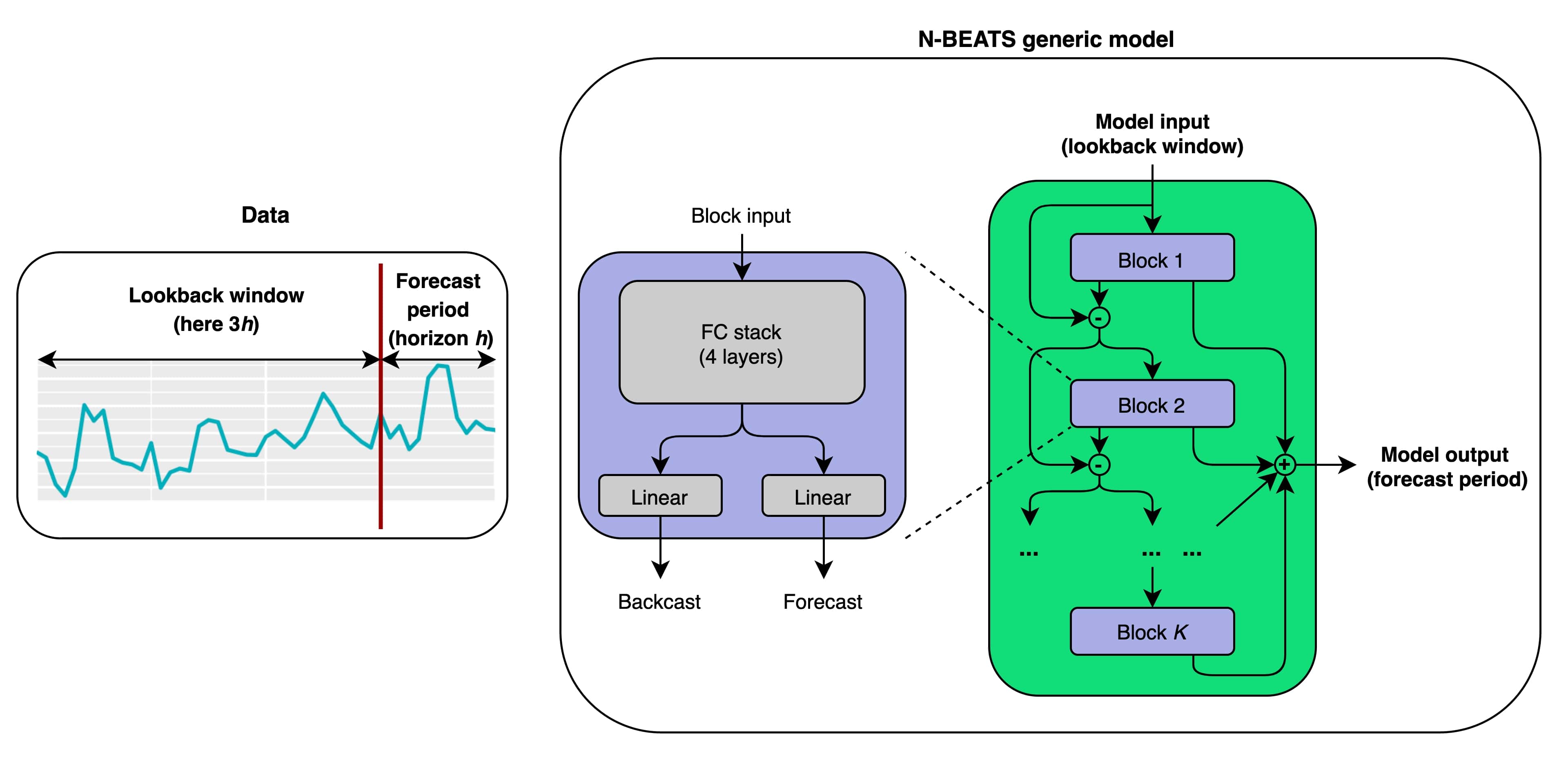
Figure 1: Generic N-BEATS architecture. Figure sourced from Van Belle et al. (2023).

To stabilize N-BEATS forecasts, Van Belle et al. (2023) propose N-BEATS-S, an N-BEATS network optimized for both forecast accuracy and stability by relying on Equation (1). More specifically, given a training set of $N$ input-output samples $\mathcal{D}=\{(\mathbf{x}^{j}_{T|t},\mathbf{y}_{h|t}^{j})\}_{j=1}^{N}$, where $\mathbf{x}^{j}_{T|t}$ contains the $T$ most recent observations at the forecasting origin $t$ ($y_{t-T+1}$ to $y_{t}$) and $\mathbf{y}_{h|t}^{j}$ contains the next $h$ observations ($y_{t+1}$ to $y_{t+h}$), they propose using an additional input-output pair $(\mathbf{x}^{j}_{T|t-1},\mathbf{y}_{h|t-1}^{j})$ for each sample $j$ in order to quantify forecast instability via $\mathcal{L}_{\text{instability}}(\hat{\mathbf{y}}_{h|t}^{j},\hat{\mathbf{y}}_{h|t-1}^{j})$, where $\hat{\mathbf{y}}_{h|t}^{j}$ and $\hat{\mathbf{y}}_{h|t-1}^{j}$ are the forecasts for sample $j$ for the input-output pairs with forecasting origins $t$ ($\hat{y}_{t+1|t}$ to $\hat{y}_{t+h|t}$) and $t-1$ ($\hat{y}_{t|t-1}$ to $\hat{y}_{t+h-1|t-1}$), respectively. The parameters $\bm{\theta}$ of an N-BEATS-S network $f(\mathbf{x};\bm{\theta})$ are then optimized as follows:

$$\bm{\theta}^{*} = \underset{\bm{\theta}}{\arg\min}\sum_{j}\bigg{[}\frac{1-\lambda}{2}\cdot\Big{(}\mathcal{L}_{\text{error}}(\mathbf{\hat{y}}_{h|t}^{j},\mathbf{y}_{h|t}^{j})+\mathcal{L}_{\text{error}}(\mathbf{\hat{y}}_{h|t-1}^{j},\mathbf{y}_{h|t-1}^{j})\Big{)}+\lambda\cdot\mathcal{L}_{\text{instability}}(\mathbf{\hat{y}}_{h|t}^{j},\mathbf{\hat{y}}_{h|t-1}^{j})\bigg{]},$$ (2)

$$\mathbf{\hat{y}}_{h|t}^{j} = f(\mathbf{x}_{T|t}^{j};\bm{\theta}),$$ (3)

$$\mathbf{\hat{y}}_{h|t-1}^{j} = f(\mathbf{x}_{T|t-1}^{j};\bm{\theta}).$$ (4)

For $\mathcal{L}_{\text{error}}$, they use the scale-independent root mean squared scaled error (RMSSE) proposed by Hyndman & Koehler (2006):

$$\text{RMSSE}(\mathbf{\hat{y}}_{h|t}^{j},\mathbf{y}_{h|t}^{j})=\sqrt{\frac{\frac{1}{h}\sum_{i=1}^{h}(y_{t+i}-\hat{y}_{t+i|t})^{2}}{\frac{1}{(T-1)}\sum_{i=1}^{T-1}(y_{t-i+1}-y_{t-i})^{2}}}.$$ (5)

For $\mathcal{L}_{\text{instability}}$, Van Belle et al. (2023) propose the root mean squared scaled change (RMSSC), defined similarly to RMSSE:

$$\text{RMSSC}(\mathbf{\hat{y}}_{h|t}^{j},\mathbf{\hat{y}}_{h|t-1}^{j})=\sqrt{\frac{\frac{1}{(h-1)}\sum_{i=1}^{h-1}(\hat{y}_{t+i|t-1}-\hat{y}_{t+i|t})^{2}}{\frac{1}{(T-1)}\sum_{i=1}^{T-1}(y_{t-i+1}-y_{t-i})^{2}}},$$ (6)

which quantifies the differences between the model forecasts made at adjacent forecasting origins for the same overlapping time periods.

2.2 Dynamic loss weighting (DLW)

In MTL, multiple tasks are trained in parallel. When these tasks are related, MTL can improve accuracy on one or more tasks compared to training a separate model for each task individually (Caruana, 1997; Ruder, 2017). In MTL with deep learning, the primary objective is generally to learn shared representations for all tasks. These shared representations are typically followed by task-specific layers for each task. Training these task-specific layers is straightforward: gradients are calculated with respect to the specific task loss, and stochastic gradient descent is used for optimization. However, training the shared layers requires combining the task-specific losses, often by taking a weighted sum of these losses (Ruder, 2017).

As explained in Section 1, the traditional approach to determining loss weights involves using grid search to find static values for these weights (Sener & Koltun, 2018). However, this method may perform poorly due to several issues identified in the literature, such as different learning speeds of the different tasks (Chen et al., 2018) and conflicting gradients (Yu et al., 2020). To address these issues, more recent works propose DLW algorithms. These algorithms leverage the iterative nature of neural network optimization by adjusting the loss weights dynamically during training, i.e., the loss weights can change throughout the process of optimizing the network parameters. Some methods specifically target the issue of varying training rates, which occurs because tasks may have different training dynamics. For instance, GradNorm (Chen et al., 2018) and Dynamic Weight Average (Liu et al., 2019) aim to balance the losses or gradients to ensure that different tasks learn at similar rates. Similarly, Kendall et al. (2018) introduce Uncertainty Weighting (UW), a method based on quantifying task uncertainty to dynamically balance task-specific losses. In contrast, Yu et al. (2020) address the problem of conflicting gradients by proposing a form of "gradient surgery" to mitigate their influence. They define two gradients to be conflicting if they point in opposite directions (i.e., have negative cosine similarity; see Section 3 for a definition). When the weighted gradient conflicts with one or more individual gradients, performance on the associated tasks will decrease. Hence, since task gradients with larger magnitude can dominate the combined gradient, this may cause the optimizer to prioritize certain tasks over others. More recently, Lin et al. (2022) proposed Random Weighting (RW), a simple yet effective approach that involves randomly sampling loss weights in each training iteration. This approach has been shown to achieve performance comparable to that of state-of-the-art techniques, including those mentioned above, on several multi-task computer vision and natural language processing problems. Consequently, the authors suggest that it should be considered a strong baseline.

A subfield within the MTL domain focuses on scenarios with one main task and one or more auxiliary tasks, with the goal of improving generalization performance on the main task. Incorporating auxiliary tasks effectively enriches the learning problem with additional training data (Caruana, 1997; Ruder, 2017). In this setting, dynamically adjusting the loss weights of the auxiliary tasks can be used to ensure that their gradients are used only if they benefit the main task’s performance. One intuitive approach is to use the auxiliary task gradient only if it has a positive cosine similarity (see Section 3 for a definition) with the main task gradient (Du et al., 2018). Lin et al. (2019) proposed an alternative method that focuses on maximizing the speed of the main task’s loss reduction. Other approaches determine the loss weights for auxiliary tasks by using a stable main task metric calculated over multiple minibatches (Verboven et al., 2023) or by employing a holdout main task metric (Grégoire et al., 2024).

Recall from Section 1 that our goal is to explore the potential of dynamically weighting the two components of the N-BEATS-S loss function during training to further improve forecast stability, compared to using static loss weights, without compromising accuracy. Given this constraint, we can approach this problem from an auxiliary task learning perspective, treating forecast accuracy as the main task and forecast stability as the auxiliary task. However, unlike traditional auxiliary task learning settings—where the final performance on auxiliary tasks is generally of lesser importance—we are explicitly interested in improving forecast stability (while either improving or at least maintaining forecast accuracy). Therefore, the problem we address in this paper can be situated between the auxiliary task learning setting and the general MTL setting.

3 Optimizing N-BEATS-S with DLW methods

The training methodology for N-BEATS-S using a DLW method to dynamically adjust the impact of forecast accuracy and forecast stability on the network parameters during training is conceptually summarized in Pseudocode 3. DLW methods differ in how they dynamically calculate $\lambda_{i}$ (line 4).

Pseudocode 1 Training N-BEATS-S with DLW.

1:for training iteration $i=1,2,\ldots$ with minibatch $\mathcal{D}_{i}$ and learning rate $\eta$ do

2:     Compute loss terms $\mathcal{L}_{\text{error}}^{i}(\mathcal{D}_{i};\bm{\theta})$ and $\mathcal{L}_{\text{instability}}^{i}(\mathcal{D}_{i};\bm{\theta})$;

3:     Compute gradients $\mathbf{g}_{\text{error}}^{i}=\nabla_{\bm{\theta}}\mathcal{L}_{\text{error}}^{i}$ and $\mathbf{g}_{\text{instability}}^{i}=\nabla_{\bm{\theta}}\mathcal{L}_{\text{instability}}^{i}$;

4:     Compute $\lambda_{i}$

5:     $\bm{\theta}\leftarrow\bm{\theta}-\eta\bigl{(}(1-\lambda_{i})\mathbf{g}_{\text{error}}^{i}+\lambda_{i}\mathbf{g}_{\text{instability}}^{i}\bigr{)}$;

6:end for

We will investigate the performance of the following existing DLW methods:

• GradNorm (Chen et al., 2018): $\lambda_{i}$ is updated to bring the gradient norms of the different tasks closer together to balance their training rates. A hyperparameter $\alpha$ controls the strength of this balancing, with higher values enforcing stronger equalization of training rates. An initial value for $\lambda_{0}$ needs to be set to initialize the algorithm.

• Uncertainty Weighting (UW) (Kendall et al., 2018): $\lambda_{i}$ is updated based on the learned relative homoscedastic uncertainties of the different tasks. A task’s homoscedastic uncertainty reflects the uncertainty inherent to the task. It is the aleatoric uncertainty (inherent randomness in the data) that stays constant for all input data but varies between different tasks. If a task’s relative homoscedastic uncertainty increases, its weight is decreased, and vice versa.

• Random Weighting (RW) (Lin et al., 2022): $\lambda_{i}$ is randomly sampled from a standard uniform distribution, $U(0,1)$.

• Gradient Cosine Similarity (GCosSim) (Du et al., 2018): $\lambda_{i}$ is either 0 or 0.5, depending on the cosine similarity between $\mathbf{g}_{\text{error}}^{i}$ (considered the main task’s gradient) and $\mathbf{g}_{\text{instability}}^{i}$ (considered the auxiliary task’s gradient), given by $\frac{\mathbf{g}_{\text{error}}^{i}\cdot\mathbf{g}_{\text{instability}}^{i}}{\|\mathbf{g}_{\text{error}}^{i}\|\|\mathbf{g}_{\text{instability}}^{i}\|}\in[-1,1]$. If the cosine similarity is negative, $\lambda_{i}=0$, and forecast instability is ignored. If the cosine similarity is positive, $\lambda_{i}=0.5$, and the gradients of both tasks are summed to update the model parameters.

• Weighted GCosSim (Du et al., 2018): This method is similar to GCosSim but accounts for the degree of similarity between $\mathbf{g}_{\text{error}}^{i}$ and $\mathbf{g}_{\text{instability}}^{i}$ (i.e., the degree to which these two vectors point in the same direction). If the cosine similarity is positive but less than one, indicating only partial alignment, $\lambda_{i}$ equals half of the cosine similarity.

Keeping in mind our goal of further improving forecast stability without compromising accuracy by optimizing N-BEATS-S with a DLW method instead of static loss weights, and considering that this problem can be situated between the auxiliary task learning setting and the general MTL setting (see Section 2.2), we propose a variant of RW to better fit this context:

• Task-Aware Random Weighting (TARW): $\lambda_{i}$ is randomly sampled from a uniform distribution, $U(0,\kappa)$, where $\kappa\in(0,1]$ is a tunable hyperparameter that caps the maximum value of the uniform distribution, preventing excessively high weights from being assigned to forecast instability. Note that $\kappa$ remains the same over all iterations.

Where RW can be seen as the stochastic version of equal weighting (where each task is assigned the same weight) (Lin et al., 2022), TARW can be considered the stochastic version of static loss weight tuning. Instead of treating $\lambda$ as a static hyperparameter, we obtain dynamic loss weights ($1-\lambda_{i}$) and $\lambda_{i}$ by tuning the hyperparameter $\kappa$, which characterizes the uniform distribution from which the weights are sampled.

4 Experimental design

In this section, we provide a detailed description of the experimental design. We begin by describing the data sets and the evaluation scheme used. Next, we present an overview of the forecasting methods included for comparison in our study and briefly outline the adopted training methodology. Finally, we explain how the hyperparameter values were obtained. The code to reproduce the experiments is available online at https://github.com/daan-caljon/Dynamic-N-BEATS-S.

4.1 Data sets

We use the monthly time series from the M3 (Makridakis & Hibon, 2000) and M4 (Makridakis et al., 2020) data sets, with summary statistics presented in Table 1. All series have positive observed values at every time step.

Table 1: Summary statistics of the data sets used.

	M3 monthly	M4 monthly
No. of series	1,428	48,000
Min. length	66	60
Max. length	144	2812
Mean length	117.3	234.3
Std. dev. length	28.5	137.4

In both the original M3 and M4 competitions, participants were tasked with generating one- to 18-month-ahead out-of-sample forecasts from a single forecasting origin. Specifically, the test set included the last 18 data points of each time series (Makridakis & Hibon, 2000; Makridakis et al., 2020). We follow this setup and use the same test set to report performance metrics.

4.2 Evaluation scheme

We adopt the evaluation scheme used by Van Belle et al. (2023) to be able to evaluate forecast stability in addition to forecast accuracy: for both data sets, a rolling forecasting origin evaluation (Tashman, 2000) is performed for each time series, in which one- to six-month-ahead forecasts from 13 consecutive forecasting origins are evaluated (so as to use the full test set, i.e., the last 18 observations of each time series). The results presented in Section 5 are averaged across (different pairs of) forecasting origins and then averaged again across all time series.

To evaluate forecast accuracy, we use the scale-independent symmetric mean absolute percentage error (sMAPE), as used in the M3 and M4 competitions (Makridakis & Hibon, 2000; Makridakis et al., 2020):

$$\text{sMAPE}(\mathbf{\hat{y}}_{h|t}^{j},\mathbf{y}_{h|t}^{j})=\frac{200}{h}\sum_{i=1}^{h}\frac{|y_{t+i}-\hat{y}_{t+i|t}|}{|y_{t+i}|+|\hat{y}_{t+i|t}|}.$$ (7)

For forecast stability, we report the scale-independent symmetric mean absolute percentage change (sMAPC) proposed by Van Belle et al. (2023), which is defined similarly to sMAPE:

$$\text{sMAPC}(\mathbf{\hat{y}}_{h|t}^{j},\mathbf{\hat{y}}_{h|t-1}^{j})=\frac{200}{(h-1)}\sum_{i=1}^{h-1}\frac{|\hat{y}_{t+i|t-1}-\hat{y}_{t+i|t}|}{|\hat{y}_{t+i|t-1}|+|\hat{y}_{t+i|t}|}.$$ (8)

It quantifies the differences between forecasts made at adjacent forecasting origins $t$ and $t-1$ for the same overlapping time periods $t+1,\dots,t+h-1$.

4.3 Forecasting methods

Alongside the results for N-BEATS-S optimized using the various DLW methods discussed in Section 3, we also report results for the following methods:

• N-BEATS: A standard N-BEATS model as described in Oreshkin et al. (2020). To fairly compare N-BEATS and N-BEATS-S forecasts, we also use the additional input-output pairs for the N-BEATS model (even though they are strictly unnecessary), with $\lambda$ set to zero to ignore the instability loss term.

• N-BEATS-S: N-BEATS-S with a static value for $\lambda$ (Van Belle et al., 2023).

• ETS: An automatically selected exponential smoothing model using the ets() function from the forecast R package (Hyndman et al., 2008, 2020).

• ARIMA: An automatically selected ARIMA model using the auto.arima() function from the forecast R package (Hyndman & Khandakar, 2008).

• THETA: The method proposed by Assimakopoulos & Nikolopoulos (2000), which won the M3 competition (Makridakis & Hibon, 2000). Forecasts are obtained using the thetaf() function from the forecast R package.

As in Van Belle et al. (2023), for each N-BEATS(-S) variant, we run the network with its specific set of hyperparameter values five times, each with a different initialization. The medians of the forecasts from these runs are then used as the final forecasts.

4.4 Training methodology for N-BEATS(-S) networks

Although we use sMAPE and sMAPC for evaluation purposes (as these metrics are convenient for comparing methods), we use RMSSE and RMSSC for the forecast error and instability loss terms, respectively, due to numerical instabilities resulting from the use of sMAPE and sMAPC. Moreover, since high levels of forecast instability are particularly undesirable and should therefore incur a relatively high cost, using a quadratic loss function for forecast instability is preferable. Using these scale-independent loss functions also eliminates the need for data preprocessing.

All networks are implemented in PyTorch (Paszke et al., 2019), and we use the Adam optimizer with default settings (Kingma & Ba, 2014) and initial learning rates as specified in Table 2 to optimize the networks’ parameters. To construct training batches, following Van Belle et al. (2023), we first sample time series uniformly at random. Next, to obtain an input-output sample for each selected time series, we sample a time step uniformly at random from the forecasting origin range. This range comprises the most recent observations that do not result in missing values when creating a sample, and its size is a hyperparameter.

4.5 Hyperparameters for N-BEATS(-S) networks

Table 2 provides an overview of the hyperparameter values used for training the N-BEATS(-S) networks, which are the tuned values reported in Van Belle et al. (2023).

Table 2: Hyperparameters for N-BEATS(-S) networks from Van Belle et al. (2023).

	M3 monthly		M4 monthly
No. of blocks $K$	20		20
Hidden layer width	256		256
Batch size	512		512
Lookback window length $T$	6$h$		4$h$
Forecasting origin range	20$h$		10$h$
Iterations	8,000		14,415
Learning rates	1e-5		1e-3
$\lambda_{\text{static}}$	0.15		0.15

For all N-BEATS-S networks optimized using DLW methods in this study, only the additional hyperparameters (if any), the learning rate, and the number of learning iterations are tuned, while the other hyperparameters are set to the values listed in Table 2. The learning rate is retuned because some methods exhibit unstable training curves with the values reported in Table 2. The number of iterations is also adjusted for two reasons: (i) a lower learning rate may require more iterations for the model to converge, and (ii) more advanced DLW methods might need additional iterations or data to achieve convergence. These hyperparameters are optimized using grid search and selected based on the minimum validation sMAPE (for converged validation losses) from a single run. The validation sMAPE is calculated on a holdout set comprising the 18 observations immediately preceding the first data point in the test set for each time series. The rolling origin evaluation procedure used for the test set results is also applied to obtain validation set results. An overview of the selected hyperparameter values is provided in Table 3.

Table 3: Hyperparameters for optimizing N-BEATS-S with DLW methods.

	M3 monthly				M4 monthly
	Iterations	Learning rate	Other		Iterations	Learning rate	Other
GradNorm	8,000	1e-5	$\alpha=0$; $\lambda_{0}=0.05$		14,415	1e-3	$\alpha=1.5$; $\lambda_{0}=0.05$
UW	10,000	1e-5	$\lambda_{0}=0.5$		14,415	1e-5	$\lambda_{0}=0.5$
RW	9,000	1e-5			18,600	1e-4
GCosSim	8,000	1e-5			14,415	1e-3
Weighted GCosSim	8,000	1e-5			14,415	5e-4
TARW	9,000	1e-5	$\kappa=0.35$		23,808	1e-3	$\kappa=0.35$

After the hyperparameters are tuned, the networks are trained on the entire training set, including the validation set. These trained networks are then used to generate forecasts for the test set, which are used to report performance metrics.

5 Results and discussion

In this section, we present and discuss the results of the experiments conducted to evaluate the impact of using a DLW method to train N-BEATS-S, focusing on its ability to further improve the stability of N-BEATS-S forecasts obtained with a static $\lambda$, without sacrificing forecast accuracy.

5.1 Results

Table 5.1 summarizes the test set results for the M3 and M4 monthly data sets. All DLW algorithms outperform N-BEATS-S on both data sets in terms of sMAPC, which measures forecast stability. However, our goal is to improve forecast stability while either improving or at least maintaining forecast accuracy. For the M3 data set, TARW achieves the highest accuracy among the DLW variants, outperforming both N-BEATS and N-BEATS-S. GradNorm and Weighted GCosSim also have sMAPE values close to those of N-BEATS and N-BEATS-S, while UW, RW, and GCosSim fail to maintain accuracy. For the M4 data set, the results are similar, with TARW again being the best-performing DLW variant, achieving the same sMAPE as N-BEATS-S. Although UW, RW, and GCosSim perform best in terms of stability on both data sets, they do so at the cost of considerable accuracy, making them less suitable for the problem addressed in this study. Finally, note that all DLW variants outperform the traditional time series forecasting methods (ETS, ARIMA, and THETA) in terms of stability. However, in terms of accuracy, the local ETS and THETA models outperform the deep learning models on the M3 data set. In contrast, for the larger M4 data set, all DLW variants, except UW, outperform the traditional methods.

Table 4: Forecast accuracy and stability performance on the test sets. Lower is better.
The minimum value per column is highlighted in bold.

	M3 monthly			M4 monthly
	sMAPE	sMAPC		sMAPE	sMAPC
N-BEATS	11.44	3.65		9.12	3.88
N-BEATS-S	11.38	2.61		9.11	2.95
GradNorm	11.47	1.63		9.23	2.17
UW	11.62	0.92		10.56	0.84
RW	11.64	1.06		9.76	1.22
GCosSim	11.59	1.05		9.70	1.28
Weighted GCosSim	11.41	2.07		9.18	2.40
TARW	11.37	2.38		$\mathbf{9.11}$	2.68
ETS	11.34	3.21		9.98	4.38
ARIMA	11.70	3.16		9.78	4.15
THETA	11.28	2.96		10.07	3.80

To determine whether the reported differences in sMAPE and sMAPC are statistically significant, we also present results from multiple comparisons with the best (MCB) tests (Koning et al., 2005). The MCB test calculates the average rank of each method across all time series in a data set based on a specified performance metric and constructs an interval around this average. If the intervals of two methods do not overlap, the difference between these methods is statistically significant. The results of the MCB tests are shown in Figure 2 (M3 monthly) and Figure 3 (M4 monthly), with the interval of the best method highlighted by the grey-shaded area. Additionally, all methods can be compared by examining the overlaps or gaps between their intervals.

The MCB results for the M3 data set indicate that ETS and TARW generate the most accurate forecasts in terms of average sMAPE rank, with a large group of methods, including the other traditional time series methods, N-BEATS-S, and two other DLW variants, GradNorm and Weighted GCosSim, resulting in forecasts with similar average accuracy. Moreover, the results confirm that the three DLW variants lead to statistically significant improvements in stability over N-BEATS-S with a static value for $\lambda$ (and the traditional time series methods). For the M4 data set, TARW and N-BEATS-S produce the most accurate forecasts in terms of average sMAPE rank, followed by Weighted GCosSim and GradNorm. For this dataset as well, these three DLW variants significantly outperform N-BEATS-S in terms of forecast stability.

Based on these results, we can conclude that GradNorm, Weighted GCosSim, and TARW further improve forecast stability compared to N-BEATS-S without considerably compromising forecast accuracy. Among these three DLW variants, TARW performs best in terms of accuracy but yields the smallest improvements in stability.

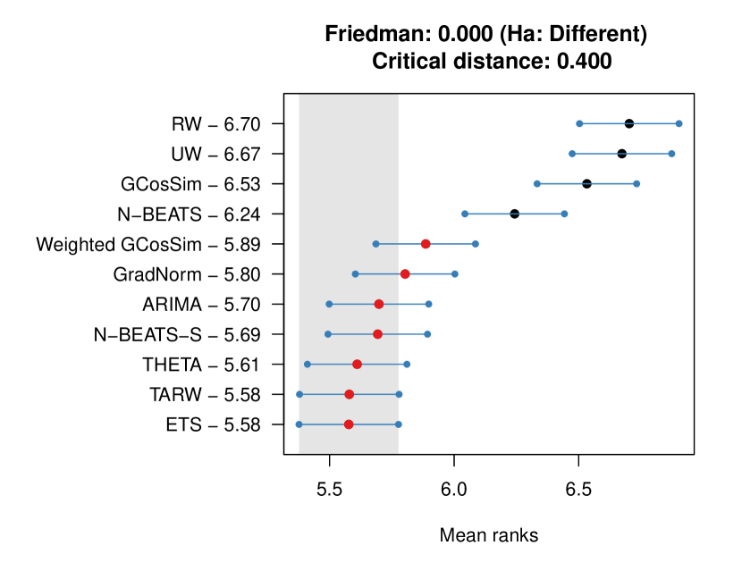
(a) sMAPE ranking

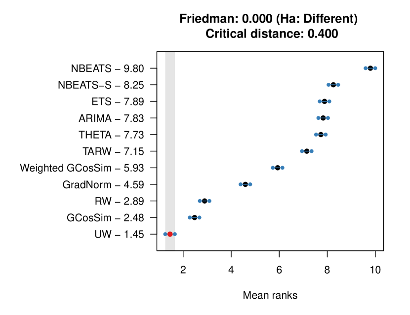
(b) sMAPC ranking

Figure 2: MCB results for the M3 monthly data set. Lower is better. If two intervals overlap, there is no statistically significant difference between the corresponding methods. There is no statistically significant difference among N-BEATS-S, GradNorm, Weighted GCosSim, and TARW in terms of sMAPE. All DLW methods outperform N-BEATS-S in terms of sMAPC.

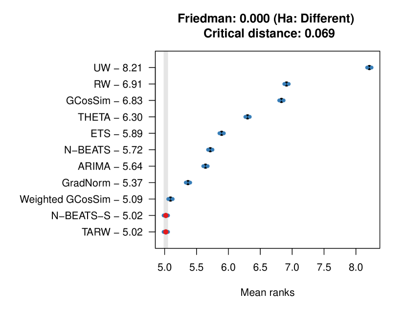
(a) sMAPE ranking

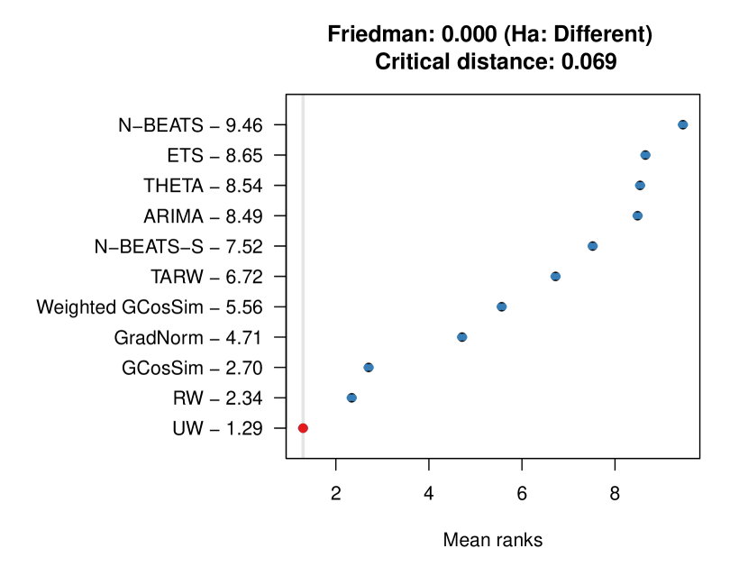
(b) sMAPC ranking

Figure 3: MCB results for the M4 monthly data set. Lower is better. If two intervals overlap, there is no statistically significant difference between the corresponding methods. There is no statistically significant difference between N-BEATS-S and TARW in terms of sMAPE. All DLW methods outperform N-BEATS-S in terms of sMAPC.

5.2 Discussion

In this section, we further investigate GradNorm, Weighted GCosSim, and TARW to gain a deeper understanding of the underlying mechanisms of these DLW methods.

5.2.1 GradNorm

Recall that the GradNorm algorithm aims to balance the training rates of the different tasks during training. Figure 4 shows the evolution of $\lambda_{i}$ during training on the M3 and M4 monthly data sets when using GradNorm.

For the M3 data set, Figure 3(a) shows that $\lambda_{i}$ decreases at the beginning of training and then gradually increases after several iterations. This pattern suggests that achieving good forecast stability early in the training process is relatively easier compared to improving accuracy, leading to a lowering of the loss weight $\lambda_{i}$ for stability to balance the training rates. After this initial learning period, $\lambda_{i}$ gradually increases and stabilizes around $0.27$, compared to $0.15$ in the static case. This supports our hypothesis regarding the usefulness of DLW methods: the model needs to achieve reasonable accuracy before it also considers forecast stability. However, for the M4 data set, this same behavior is not visible in Figure 3(b): $\lambda_{i}$ decreases only after the first iteration and then quickly increases to 0.3, where it stabilizes. An additional experiment showed that lowering the learning rate for the M4 data set results in a similar evolution of $\lambda_{i}$ as observed for the M3 data set, whereas with the higher learning rate, a reasonable accuracy is already achieved after the first iteration.

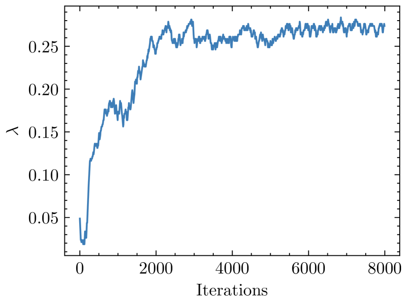
(a) M3 monthly

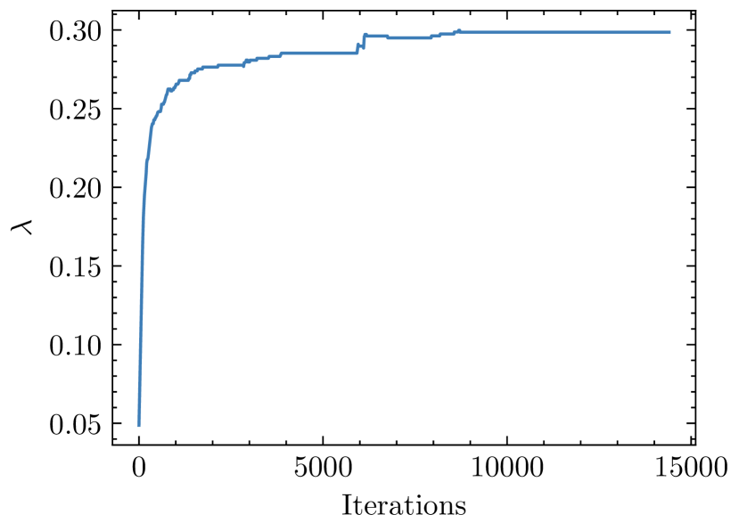
(b) M4 monthly

Figure 4: Evolution of $\lambda_{i}$ during training using GradNorm.

5.2.2 Weighted GCosSim

Figure 5 shows the evolution of the cosine similarity between $\mathbf{g}_{\text{error}}^{i}$ and $\mathbf{g}_{\text{instability}}^{i}$ during training with Weighted GCosSim on the M3 and M4 monthly data sets. There are two important observations to discuss. First, for both data sets, the cosine similarity is generally greater than zero throughout training. This confirms that optimizing for forecast accuracy and forecast stability can be considered related tasks (after all, if a model generates perfect zero-error forecasts, these forecasts will also be perfectly stable by definition). Consequently, forecast instability is (almost) consistently taken into account during training with Weighted GCosSim. The fact that the cosine similarity is substantially less than one for most of the training may explain why regular GCosSim leads to poor accuracy performance. Since regular GCosSim essentially adds the gradients for both tasks in each iteration without considering the degree of similarity between them, it places too much emphasis on forecast instability given our goal of improving stability without sacrificing accuracy. Second, for the M3 data set, Figure 4(a) shows that the cosine similarity is close to zero at the start of training, indicating that accuracy and stability are initially unrelated according to cosine similarity. As training progresses, the cosine similarity becomes positive, suggesting that these tasks become related after this initial phase. This aligns with the observed evolution of $\lambda_{i}$ for GradNorm: both algorithms prioritize optimizing forecast accuracy at the start of training before considering forecast instability. However, as with GradNorm, this behavior is not visible for the M4 data set (see Figure 4(b)). This can again be attributed to the higher learning rate used for M4, which leads to a reasonable accuracy after just the first iteration.

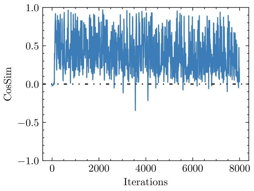
(a) M3 monthly

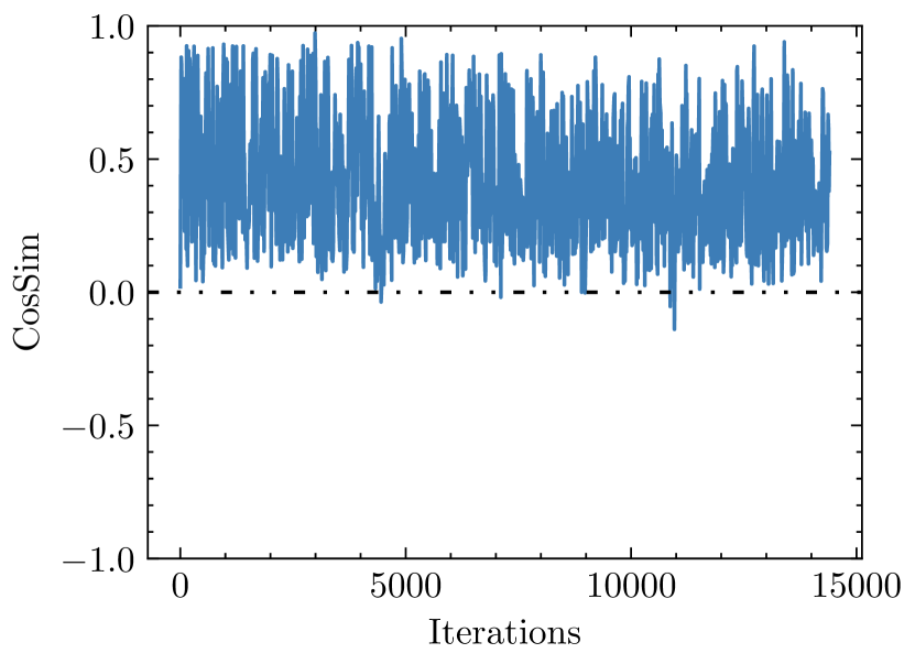
(b) M4 monthly

Figure 5: Evolution of cosine similarity between $\mathbf{g}_{\text{error}}^{i}$ and $\mathbf{g}_{\text{instability}}^{i}$ during training using Weighted GCosSim.

5.2.3 TARW

Figure 6 illustrates how validation accuracy (sMAPE) and stability (sMAPC) for TARW vary as a function of the hyperparameter $\kappa$ for both the M3 and M4 monthly data sets. As $\kappa$ increases, a greater average weight is assigned to forecast instability during training. The impact of $\kappa$ on sMAPE and sMAPC is similar across both data sets, following trends consistent with those observed for a static $\lambda$ in Van Belle et al. (2023). While sMAPC shows an almost linear decrease with increasing $\kappa$, sMAPE initially decreases to a minimum and then increases as $\kappa$ continues to rise (supporting the idea that incorporating forecast instability in training can act as a regularization mechanism). As discussed in Section 4.5, the minimum validation sMAPE is used to select $\kappa$, resulting in $\kappa=0.35$ for both data sets. Interestingly, this choice leads to $\mathbb{E}[\lambda_{i}]>\lambda_{\text{static}}$, which may (partly) explain the further improvement in forecast stability compared to N-BEATS-S. Additionally, we conjecture that TARW, as the stochastic version of static loss weight tuning (see Section 3), outperforms the latter because it can explore the loss space more effectively and may better escape local optima due to its stochastic nature.

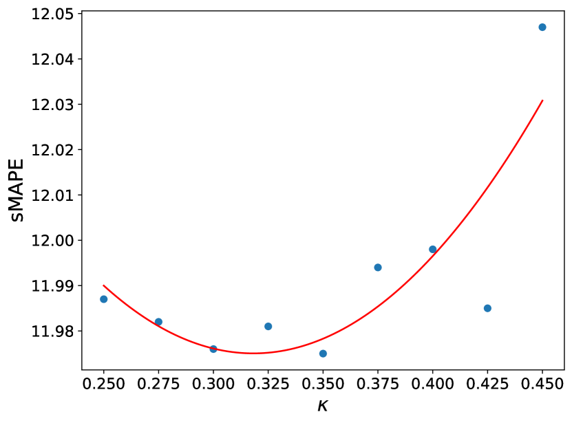
(a) Accuracy for M3 monthly

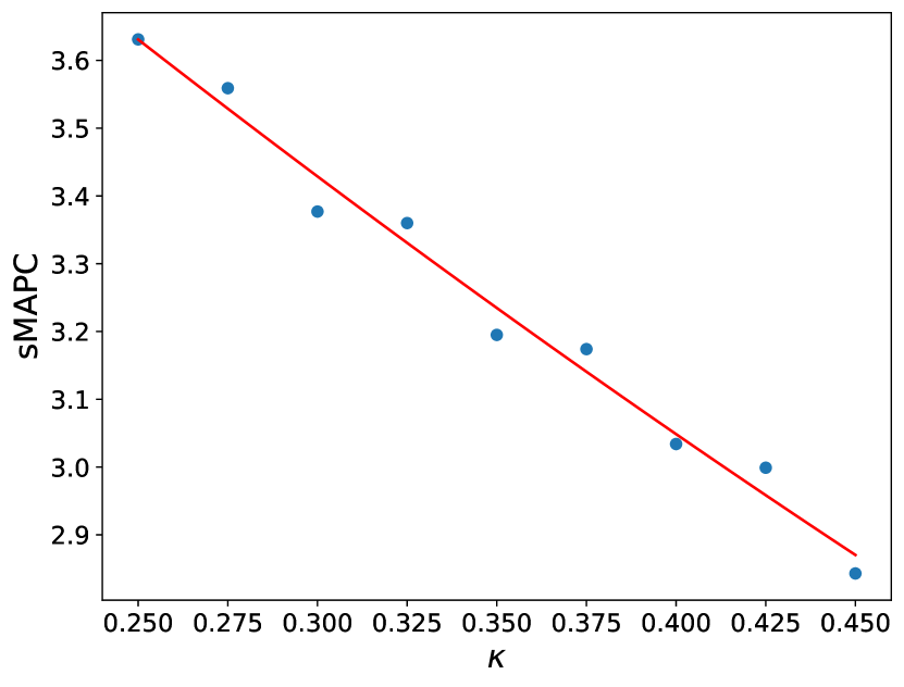
(b) Stability for M3 monthly

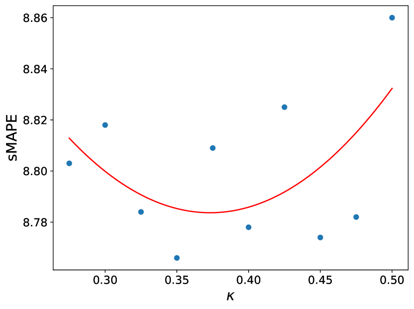
(c) Accuracy for M4 monthly

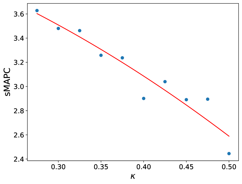
(d) Stability for M4 monthly

Figure 6: Validation accuracy (sMAPE) and stability (sMAPC) for TARW as a function of its hyperparameter $\kappa$.

6 Conclusions and future research

Rolling origin forecast instability can incur costs, as updates to forecasts based on new data may require changes to plans that rely on these forecasts as inputs. Van Belle et al. (2023) propose a methodology to optimize global neural point forecasting models from both a forecast accuracy and stability perspective, aiming to improve forecast stability while maintaining accuracy. They apply this methodology to extend the N-BEATS method (Oreshkin et al., 2020), resulting in a new method called N-BEATS-S.

In this paper, we explore the potential of using DLW methods to train N-BEATS-S, with the goal of further improving forecast stability while either improving or at least maintaining forecast accuracy compared to N-BEATS-S with static tuned loss weights. To this end, we use existing DLW algorithms and propose TARW, a variant of RW (Lin et al., 2022), specifically tailored to align with our objective. Our empirical results on the M3 and M4 monthly data sets demonstrate that training N-BEATS-S using certain DLW methods can outperform N-BEATS-S with static tuned loss weights in terms of further improving forecast stability without a significant trade-off in accuracy.

The motivation for using DLW methods stems from the hypothesis that forecast accuracy should be prioritized in the early stages of training, with forecast instability being addressed only after a reasonable level of accuracy has been achieved. This approach may lead to better results by enabling a more targeted exploration of the loss space, more closely aligned with our goal. Our experiments with GradNorm (see Section 5.2.1) and Weighted GCosSim (see Section 5.2.2) support this hypothesis. Additionally, training N-BEATS-S using TARW also yields favorable results, even outperforming the aforementioned DLW methods in terms of accuracy. While TARW does not directly prioritize accuracy in the early stages of training but instead randomly samples loss weights from a uniform distribution $U(0,\kappa)$, where $\kappa\in(0,1]$ is a tunable hyperparameter, we believe this stochastic variant of static loss weight tuning is effective because it allows for a more comprehensive exploration of the loss space and may better escape local optima due to its stochastic nature.

One limitation of this work is that we only incorporate forecast stability for adjacent forecasting origins during optimization (as in Van Belle et al. (2023)). While it is intuitive that this approach would also improve stability for non-adjacent forecasting origins, the effectiveness of directly accounting for instability with respect to non-adjacent origins during optimization should be explored in future work. Additionally, to further validate our findings, the benefits of training N-BEATS-S using DLW methods should be tested on a broader range of data sets. Another limitation of our study is the ensemble size. As explained in Section 4.3, we use ensembles consisting of only five models, whereas Oreshkin et al. (2020) used a total of 180 models for each of their final N-BEATS ensembles. Investigating how ensemble size and type affect forecast accuracy and stability is an interesting direction for future research.

Moreover, another promising area for future research is the application of TARW in other MTL settings. Given that Lin et al. (2022) demonstrated the superiority of RW over equal weighting, it is plausible that TARW could also outperform static loss weight tuning in other MTL problems due to its stochastic nature. Finally, a broader direction for future research concerns incorporating forecast stability into different modeling approaches or pipelines, such as the post-processing technique for stabilizing point forecasts proposed by Godahewa et al. (2023) or the N-BEATS variant to stabilize Gaussian probabilistic forecasts by Van Belle et al. (2024). Of particular interest is the incorporation of forecast stability into tree-based methods like LightGBM (Ke et al., 2017) due to their widespread adoption in the time series forecasting field, as evidenced in the M5 competition (Makridakis et al., 2022).

Acknowledgements

This work was supported by the Research Foundation – Flanders [grant number 12AZX24N].

References

- Assimakopoulos & Nikolopoulos (2000) Assimakopoulos, V. & Nikolopoulos, K. (2000). The theta model: a decomposition approach to forecasting. International Journal of Forecasting, 16(4), 521–530.
- Caruana (1997) Caruana, R. (1997). Multitask learning. Machine Learning, 28, 41–75.
- Chen et al. (2018) Chen, Z., Badrinarayanan, V., Lee, C.-Y., & Rabinovich, A. (2018). GradNorm: Gradient normalization for adaptive loss balancing in deep multitask networks. In International Conference on Machine Learning, (pp. 794–803). PMLR.
- Du et al. (2018) Du, Y., Czarnecki, W. M., Jayakumar, S. M., Farajtabar, M., Pascanu, R., & Lakshminarayanan, B. (2018). Adapting auxiliary losses using gradient similarity. arXiv preprint arXiv:1812.02224.
- Godahewa et al. (2023) Godahewa, R., Bergmeir, C., Baz, Z. E., Zhu, C., Song, Z., García, S., & Benavides, D. (2023). On forecast stability. arXiv preprint arXiv:2310.17332.
- Grégoire et al. (2024) Grégoire, E., Chaudhary, M. H., & Verboven, S. (2024). Sample-level weighting for multi-task learning with auxiliary tasks. Applied Intelligence, 54(4), 3482–3501.
- Hyndman et al. (2020) Hyndman, R., Athanasopoulos, G., Bergmeir, C., Caceres, G., Chhay, L., O’Hara-Wild, M., Petropoulos, F., Razbash, S., Wang, E., & Yasmeen, F. (2020). forecast: Forecasting functions for time series and linear models. R package version 8.13.
- Hyndman & Khandakar (2008) Hyndman, R. J. & Khandakar, Y. (2008). Automatic time series forecasting: the forecast package for R. Journal of Statistical Software, 26(3), 1–22.
- Hyndman & Koehler (2006) Hyndman, R. J. & Koehler, A. B. (2006). Another look at measures of forecast accuracy. International Journal of Forecasting, 22(4), 679 – 688.
- Hyndman et al. (2008) Hyndman, R. J., Koehler, A. B., Ord, J. K., & Snyder, R. D. (2008). Forecasting with exponential smoothing: the state space approach. Berlin: Springer-Verlag.
- Januschowski et al. (2020) Januschowski, T., Gasthaus, J., Wang, Y., Salinas, D., Flunkert, V., Bohlke-Schneider, M., & Callot, L. (2020). Criteria for classifying forecasting methods. International Journal of Forecasting, 36(1), 167–177.
- Ke et al. (2017) Ke, G., Meng, Q., Finley, T., Wang, T., Chen, W., Ma, W., Ye, Q., & Liu, T.-Y. (2017). LightGBM: A highly efficient gradient boosting decision tree. Advances in Neural Information Processing Systems, 30.
- Kendall et al. (2018) Kendall, A., Gal, Y., & Cipolla, R. (2018). Multi-task learning using uncertainty to weigh losses for scene geometry and semantics. In Proceedings of the IEEE Conference on Computer Vision and Pattern Recognition, (pp. 7482–7491).
- Kingma & Ba (2014) Kingma, D. P. & Ba, J. (2014). Adam: A method for stochastic optimization. arXiv preprint arXiv:1412.6980.
- Koning et al. (2005) Koning, A. J., Franses, P. H., Hibon, M., & Stekler, H. O. (2005). The M3 competition: Statistical tests of the results. International Journal of Forecasting, 21(3), 397–409.
- Li & Disney (2017) Li, Q. & Disney, S. M. (2017). Revisiting rescheduling: MRP nervousness and the bullwhip effect. International Journal of Production Research, 55(7), 1992–2012.
- Lin et al. (2022) Lin, B., Ye, F., Zhang, Y., & Tsang, I. W. (2022). Reasonable effectiveness of random weighting: A litmus test for multi-task learning. Transactions on Machine Learning Research.
- Lin et al. (2019) Lin, X., Baweja, H., Kantor, G., & Held, D. (2019). Adaptive auxiliary task weighting for reinforcement learning. Advances in Neural Information Processing Systems, 32.
- Liu et al. (2019) Liu, S., Johns, E., & Davison, A. J. (2019). End-to-end multi-task learning with attention. In Proceedings of the IEEE/CVF Conference on Computer Vision and Pattern Recognition, (pp. 1871–1880).
- Makridakis & Hibon (2000) Makridakis, S. & Hibon, M. (2000). The M3-competition: Results, conclusions and implications. International Journal of Forecasting, 16(4), 451–476.
- Makridakis et al. (2020) Makridakis, S., Spiliotis, E., & Assimakopoulos, V. (2020). The M4-competition: 100,000 time series and 61 forecasting methods. International Journal of Forecasting, 36(1), 54–74.
- Makridakis et al. (2022) Makridakis, S., Spiliotis, E., & Assimakopoulos, V. (2022). The M5 competition: Background, organization, and implementation. International Journal of Forecasting, 38(4), 1325–1336.
- Oreshkin et al. (2020) Oreshkin, B. N., Carpov, D., Chapados, N., & Bengio, Y. (2020). N-BEATS: Neural basis expansion analysis for interpretable time series forecasting. In International Conference on Learning Representations.
- Paszke et al. (2019) Paszke, A., Gross, S., Massa, F., Lerer, A., Bradbury, J., Chanan, G., Killeen, T., Lin, Z., Gimelshein, N., Antiga, L., et al. (2019). Pytorch: An imperative style, high-performance deep learning library. Advances in Neural Information Processing Systems, 32.
- Petropoulos et al. (2022) Petropoulos, F., Apiletti, D., Assimakopoulos, V., Babai, M. Z., Barrow, D. K., Taieb, S. B., Bergmeir, C., Bessa, R. J., Bijak, J., Boylan, J. E., et al. (2022). Forecasting: theory and practice. International Journal of Forecasting, 38(3), 705–871.
- Ruder (2017) Ruder, S. (2017). An overview of multi-task learning in deep neural networks. arXiv preprint arXiv:1706.05098.
- Sener & Koltun (2018) Sener, O. & Koltun, V. (2018). Multi-task learning as multi-objective optimization. Advances in Neural Information Processing Systems, 31.
- Tashman (2000) Tashman, L. J. (2000). Out-of-sample tests of forecasting accuracy: An analysis and review. International Journal of Forecasting, 16(4), 437–450.
- Tunc et al. (2013) Tunc, H., Kilic, O. A., Tarim, S. A., & Eksioglu, B. (2013). A simple approach for assessing the cost of system nervousness. International Journal of Production Economics, 141(2), 619–625.
- Van Belle et al. (2024) Van Belle, J., Crevits, R., Caljon, D., & Verbeke, W. (2024). Probabilistic forecasting with modified N-BEATS networks. IEEE Transactions on Neural Networks and Learning Systems.
- Van Belle et al. (2023) Van Belle, J., Crevits, R., & Verbeke, W. (2023). Improving forecast stability using deep learning. International Journal of Forecasting, 39(3), 1333–1350.
- Verboven et al. (2023) Verboven, S., Chaudhary, M. H., Berrevoets, J., Ginis, V., & Verbeke, W. (2023). Hydalearn. Applied Intelligence, 53, 5808–5822.
- Wei et al. (2022) Wei, T., Wang, S., Zhong, J., Liu, D., & Zhang, J. (2022). A review on evolutionary multitask optimization: Trends and challenges. IEEE Transactions on Evolutionary Computation, 26(5), 941–960.
- Yu et al. (2020) Yu, T., Kumar, S., Gupta, A., Levine, S., Hausman, K., & Finn, C. (2020). Gradient surgery for multi-task learning. Advances in Neural Information Processing Systems, 33, 5824–5836.