Bayesian Event Categorization Matrix Approach for Nuclear Detonations

Abstract

Current efforts to detect nuclear detonations and correctly categorize explosion sources with ground- and space-collected discriminants presents challenges that remain unaddressed by the Event Categorization Matrix model. Smaller events (lower yield explosions) often include only sparse observations among few modalities and can therefore lack a complete set of discriminants. The covariance structures can also vary significantly between such observations of event (source-type) categories. Both obstacles are problematic for the “classic” Event Categorization Matrix model. Our work addresses this gap and presents a Bayesian update to the previous Event Categorization Matrix model, termed the Bayesian Event Categorization Matrix model, which can be trained on partial observations and does not rely on a pooled covariance structure. We further augment the Event Categorization Matrix model with Bayesian Decision Theory so that false negative or false positive rates of an event categorization can be reduced in an intuitive manner. To demonstrate improved categorization rates for the Bayesian Event Categorization Matrix model, we compare an array of Bayesian and classic models with multiple performance metrics using Monte Carlo experiments. We use both synthetic and real data. Our Bayesian models show consistent gains in overall accuracy and a lower false negative rates relative to the classic Event Categorization Matrix model. We propose future avenues to improve Bayesian Event Categorization Matrix models for further improving decision-making and predictive capability.

Keywords— Bayesian inference, Monte Carlo methods, Probability distributions, Statistical methods, Earthquake monitoring and test-ban treaty verification

1 Introduction

The central question in the discussion of an adequate monitoring of a [comprehensive test ban treaty] is that of confidently identifying seismic events, i. e., to judge whether observed seismic signals are generated by an underground nuclear explosion or by an earthquake.

[14]
[14]

Statistical methods have historically supported monitoring signatures of suspected nuclear explosions [10, 5]. Agencies that verify test ban treaties, in particular, leverage such methods to confirm or challenge the hypotheses that some geophysical events present evidence of a nuclear detonation, rather than natural processes [40]. Such methods have been crucial in seismic source identification, that is, statistical methods that screen explosion-sourced records of seismic activity from records expected from earthquakes or other processes.

Early quantitative work [9] that developed classification methods to separate explosions from earthquake populations (discrimination) in the 1960s justified later efforts to rigorously defend test-ban treaties [16]. Some of these treaties were only aspirational at the time that the geophysical work was achieved [42, 15]. More modern efforts from researchers like Shumway [50, 52, 51], Anderson [4, 5, 6, 1], and their coworkers [31] have further advanced these statistical methods beyond discrimination. Such newer methods often ingest multiple discriminants [17, 3] or other modalities [44] in statistical tests that screen all-source explosions from earthquakes. Some recent research has continued the trend to use data integration or fusion methods to more confidently detect [49, 11, 12], identify [54, 7], and characterize [18, 20, 26, 57] populations of explosions from other events, and thereby reduce false positive rates. This effort continues to focus on smaller, evasively conducted explosions [36, 47].

One such multi-discriminant, statistical method that supports test ban treaty verification is called the Event Categorization Matrix [3, ECM,]. This method has historically been used to test if multiple observations associated with a single event support the hypothesis that their source was a nuclear detonation [39]. The ECM method currently consumes seismic discriminants like event depth, ratios of body-wave and surface-wave magnitudes, and ground motion polarity. Some variants of ECM also leverage more novel discriminants, like infrasound phase arrivals and teleseismic waveform complexity factors (CFs) [2]. Such populations of discriminants that are sourced by nuclear detonations largely segregate from populations that are sourced by nuisance events that form other categories, like shallow earthquakes and mining explosions.

The ECM method assumes that a vector of discriminant observations can be modeled as a random variable from a multivariate normal distribution, with a mean and covariance matrix specific to a single event category. The ECM method uses previous observations with known event categories (ground truth data) to estimate mean and covariance parameters for each event category distribution, and applies regularized discriminant analysis [21, RDA,] to estimate covariance matrices for small data sets. The ECM model then categorizes a new observation with a series of hypothesis tests that are based on typicality indices [41], and quantifies the likely set membership of the new, uncategorized, observation to each candidate event group. If a new observation is atypical of all categories, with the exception of the nuclear detonation category, its source is then categorized as a nuclear explosion.

While technologies to monitor for nuclear explosions leverage multiple sensor networks (e.g., satellites and seismic arrays) research to routinely fuse such multi-modal, simultaneous observations and improve event categorization accuracy remains on-going [29, 34]. Both physical and mathematical issues each challenge implementing ECM with multiple modalities [3].

Firstly, it is operationally difficult to associate multi-modal signals to the same causative source for all but the largest events. Therefore, analyses of such data can produce limited sets of discriminants. This means that the ECM model, which must use the same set of discriminants that it is calibrated against to categorize a new event, cannot ingest data from a new event that contains only partial observations, relative to that calibration data.

Secondly, ECM uses a covariance estimator which can lead to model mis-specification, because there is the potential for events that produce multi-modal signals to have a drastically different covariance structures. For example, high-yield, aboveground nuclear detonations will produce optical signals with high irradiance that covaries with large amplitude seismic waveforms [19]. This does not imply that a nuisance event that produces a high irradiance signal (like cloud-to-cloud lightning) will also produce seismic waveforms with significant amplitude. Therefore, while the nuclear detonation may produce covarying discriminants, nuisance events may not.

Lastly, ECM may categorize an event for non-intuitive reasons. This is particularly true when the number of event categories considered grows. When ECM then fails to reject a new observation from multiple event categories, the model declares the event as indeterminate, requiring human intervention for categorization [3]. A monitoring agent must then explore strategies to empirically reduce the observed number of false negatives, while not significantly increasing the number of indeterminate categorizations or the overall categorization accuracy. Some of the gaps in [3]’s [*]anderson2007mathematical approach are a result of hypothesis testing and parameter estimation procedures associated with classical statistical methods. Hence, subsequent references to the ECM model provided in [3] are termed classical ECM (C-ECM).

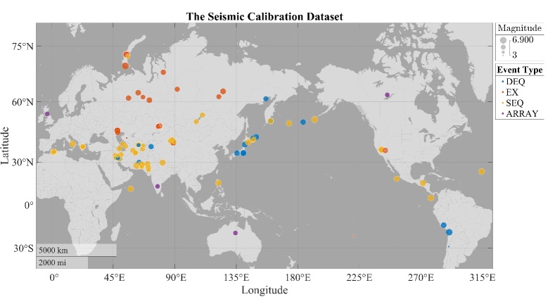
Figure 1: The source locations for ground truth (calibration) dataset for C-ECM and each form of B-ECM, across the globe. Many sources were recorded from historical nuclear tests and their size is marked by seismic magnitude (see legend). Explosions with entirely missing magnitude data are marked with a “magnitude 3” size marker; this provides a crude estimate for global magnitude of completeness in most continental regions. The violet circles mark locations of the the four seismic arrays (labeled “ARRAY”) that provided the bulk of the discriminant data.

To address some of the problems faced with fusing discriminants from multiple modalities, we develop an ECM model which uses Bayesian methods (B-ECM) for parameter estimation and decision criteria. This novel work uses Bayesian decision theory and treats missing data with a matrix $t$-distribution within a Bayesian Normal mixture model [53]. We evaluate integrals analytically when possible to avoid the computational expense of multi-dimensional numerical integration. These collective advances then select an event category for a new observation within practical time constraints and without supervision. We utilize a Bayesian typicality index to detect if a new observation is inconsistent with the event categories used for training, under the uncertainty imparted by using training data with missing elements. Lastly, we demonstrated the accuracy of the B-ECM methodology against a carefully prepared, curated dataset with missing entries (Fig. 1), which C-ECM has previously been demonstrated against [2]. This establishes a baseline and measures gains in accuracy with the same curated dataset.

We organize this report as follows: Section 2 summarizes the statistical methods assimilated to create the B-ECM methodology. Section 3 overviews how these methods are implemented in codes and algorithms. Section 4 details results from a series of Monte Carlo (MC) experiments that compare the performance of the B-ECM models versus the C-ECM model. Finally, section 5 provides a discussion of the results, their implications, and potential avenues for further improvements to event categorization models.

2 Statistical Basis for the Decision Framework

B-ECM is an end-to-end formalized framework that exploits geophysical discriminants to categorize an unknown event. We use Bayesian inference (Section 2.1) throughout this work to ensure consistency between the computational and data processing stages of B-ECM. Our statistical model (Section 2.2) leverages Bayesian inference to use training data with missing discriminants. Bayesian decision theory (Section 2.3) enables consistent decision making, taking into account category probabilities, the utility of a correct categorization, and the loss of an incorrect categorization. Notation is detailed in Nomenclature Appendix A.

2.1 Bayesian Inference

Bayesian statistics relies on Bayes’ Theorem (Equation 1) to infer model parameters. Bayes’ rule reads as: the posterior distribution of $\phi$ given data $y$; $p(\phi|y)$, is equal to the likelihood of the data $p(y|\phi)$ times the prior distribution on the model parameter $p(\phi)$, divided by the marginal likelihood of the data $p(y)$:

$$p(\phi|y)=\frac{p(y|\phi)p(\phi)}{p(y)}$$ (1)

Bayesian inference treats probability as model parameter uncertainty, resulting in a probability distribution on $\phi$ instead of a point estimate. Computational methods, like the Gibbs sampler, often use Markov chain Monte Carlo (MCMC) to infer model parameters by sampling model parameters from the posterior distribution $p\left(\phi|y\right)$ [23, 22, 13, 25]. An observer can consider the probabilities for multiple models, given the data, to make data predictions under the Bayesian framework. We use these traits of Bayesian inference to derive B-ECM. [30] provdies more resources on Bayesian inference and [45] gives more details about MCMC and statistical simulation.

2.2 Bayesian Categorization with Missing Training Data

We choose to categorize data with a methodology that is similar to that in [53]. This method assumes that the event category for each training data event known, but the group for which a new observation belongs to is unknown. We let $\bm{Y}_{N\times p}$ be a matrix that contains the entirety of the training data, with $N$ event observations each with $p$ observed discriminants. Each row of $\bm{Y}_{N\times p}$ is an observation of the $k^{\mathrm{th}}$ event category, where $k\in\{1,\dots,K\}$ has no uncertainty. We split the training data into the event category-specific matrices $\bm{Y}_{N_{1}\times p},\dots,\bm{Y}_{N_{k}\times p},\dots,\bm{Y}_{N_{K}\times p}$. Here, $N_{k}$ is the number of training observations in the $k^{\mathrm{th}}$ event category and $N_{1}+\dots+N_{k}+\dots+N_{K}=N$. The $p$ discriminants in each $\bm{Y}_{N_{k}\times p}$ are the same and are arranged in the same column order.

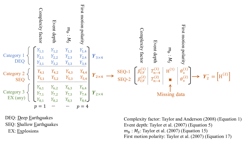
Figure 2: A visual description of the training data $\bm{Y}_{N\times p}$ that populates the B-ECM module. Dimensions $N=8$ and $p=4$ in this example. The top, leftmost column matrix organizes data within three categories (deep earthquakes, shallow earthquakes, and explosions) into distinct groups of rows. The four columns enumerate distinct seismic discriminant types (complexity factor, event depth, body wave to surface wave magnitudes, and polarity of first motion). The row matrices $\bm{Y}_{N_{k}\times p}$ compartmentalize this training data by category, which we color separately. The sub-matrix $\bm{Y}_{2\times 4}$ $(N_{2}=2,p=4)$ then stores data observed from shallow earthquakes (SEQ), according to the notation cited at the bottom right. The second shallow earthquake observation lacks a body wave to surface wave magnitude measurement. This missing data then populates the data set $\bm{Y}_{2}^{-}$.

We assume that each $\bm{Y}_{N_{k}\times p}$ is a realization from a Matrix Normal distribution [27], with an unknown mean $\bm{1}_{N_{k}}\bm{\mu}_{k}^{\top}$, independent rows, and column covariance $\bm{\Sigma}_{k}$. Appendix LABEL:sec:normal-likelihood provides details. The elements of a Matrix Normal distributed random variable have infinite support (that is, the interval where the density is not identically zero) on the real number line. Historically, p-values on $(0,1]$ have been used with ECM [3]. We choose to transform these values with a logit transformation $\mathrm{logit}(x)=\mathrm{ln}(x)-\mathrm{ln}(1-x)$ so that the transformed values are (instead) unbounded. The arcsine transform used in [3] returns values on $[0,1]$ instead of on the entire real number line. This property is a mis-match for the normal distribution, which has support for all real numbers. However, both transforms are available for use in our code.

We integrate the Matrix Normal density of each $\bm{Y}_{N_{k}\times p}$ over the prior densities of $\bm{\mu}_{k}$ and $\bm{\Sigma}_{k}$ for each $k$ analytically. This reduces the computational burden of inference, as detailed in Appendix LABEL:sec:data-likelihood. Integration results in the marginal likelihood $p(\bm{Y}_{N_{k}\times p}|\bm{\theta}_{k})$, which is a matrix t-distribution [27], conditioned on a set of prior hyperparameters, abbreviated as $\bm{\theta}_{k}$ for the hyperparameters specific to group $k$. We refer to the set of prior hyperparameters, totaled over all $K$ event categories, as $\bm{\theta}$. Appendix LABEL:sec:priors details the prior distributions and hyperparameters in $\bm{\theta}$. Appendix LABEL:sec:matrix-t provides relevant properties of the matrix t-distribution.

Sometimes an event contained in $\bm{Y}_{N_{k}\times p}$ will have less than $p$ recorded discriminants, which is therefore unavailable. The unavailable discriminants for such a case are considered missing data [38, 24]. We let $\bm{Y}_{k}^{-}$ represent the missing data elements from all $N_{k}$ events in $\bm{Y}_{N_{k}\times p}$ and $\bm{Y}_{k}^{+}$ be the recorded elements, respectively. We leave $\bm{Y}_{k}^{+}$ and $\bm{Y}_{k}^{-}$ dimensionless to represent the observed and missing data with generality. We use the chain rule of conditional probability to specify

$$p(\bm{Y}_{N_{k}\times p}|\bm{\theta}_{k})=p(\bm{Y}_{k}^{-},\bm{Y}_{k}^{+}|\bm{\theta}_{k})=p(\bm{Y}_{k}^{-}|\bm{Y}_{k}^{+},\bm{\theta}_{k})p(\bm{Y}_{k}^{+}|\bm{\theta}_{k}).$$ (2)

Because of the properties of conditional probability and $p(\bm{Y}_{N_{k}\times p}|\bm{\theta}_{k})$, we can obtain a large number of random draws, or samples, of $\bm{Y}_{k}^{-}$ given $\bm{Y}^{+}_{k}$ and $\bm{\theta}_{k}$ from the probability density function $p(\bm{Y}_{k}^{-}|\bm{Y}_{k}^{+},\bm{\theta}_{k})$ using a combination of conditional formulas (Appendices LABEL:sec:matrix-t and LABEL:sec:missing-data-conditionals) for the matrix t-distribution and numerical methods. We use these probabilistic imputations of $\bm{Y}_{k}^{-}$ to exploit partial observations in the training data set, and thereby compute more accurate decisions by utilizing instead of discarding partial observations.

We now use the imputed $\bm{Y}_{k}^{-}$ and return to a full data set $\bm{Y}_{N_{k}\times p}$ and $p(\bm{Y}_{N_{k}\times p}|\bm{\theta}_{k})$ to next quantify the uncertainty that a new event belongs to each training category. We then let $\tilde{\bm{y}}_{\tilde{p}}$ be such a new event recorded as a vector of discriminants of length $\tilde{p}\leq p$. Vector $\tilde{\bm{y}}_{\tilde{p}}$ is associated with the random vector of length $K$ that we call $\tilde{\bm{z}}_{K}^{\top}=[\tilde{z}_{1},\dots,\tilde{z}_{k},\dots,\tilde{z}_{K}]$. A random realization of $\tilde{\bm{z}}_{K}$ is equivalent to a draw from a multinomal distribution for $n=1$, where a single element is equal to 1 and the remaining elements are zero. The index, $k\in\{1,\dots,K\}$, of the non-zero value of $\tilde{\bm{z}}_{K}$, corresponds to $\tilde{\bm{y}}_{\tilde{p}}$ belonging to the $k^{\mathrm{th}}$ training event category. The conditional expected value of $\tilde{\bm{z}}_{K}$, given all the data and prior parameter specifications, is then equivalent to:

$$\mathbb{E}[\tilde{\bm{z}}_{K}|\tilde{\bm{y}}_{\tilde{p}},\bm{Y}_{N\times p},\bm{\theta}]=[p(\tilde{z}_{1}=1|\tilde{\bm{y}}_{\tilde{p}},\bm{Y}_{N\times p},\bm{\theta}),\dots,p(\tilde{z}_{K}=1|\tilde{\bm{y}}_{\tilde{p}},\bm{Y}_{N\times p},\bm{\theta})].$$ (3)

Equation 3 is equivalent to a vector that specifies the probability of $\tilde{\bm{y}}_{\tilde{p}}$ belonging to each of the $K$ event categories. For the $k^{\mathrm{th}}$ event category, $p(\tilde{z}_{k}=1|\tilde{\bm{y}}_{\tilde{p}},\bm{Y}_{N\times p},\bm{\theta})$ can be evaluated using Bayes’ rule.

$$p(\tilde{z}_{k}=1|\tilde{\bm{y}}_{\tilde{p}},\bm{Y}_{N\times p},\bm{\theta})=\frac{p(\tilde{\bm{y}}_{\tilde{p}}|\tilde{z}_{k}=1,\bm{Y}_{N_{k}\times p},\bm{\theta}_{k})p(\tilde{z}_{k}=1|\bm{Y}_{N\times p},\bm{\theta})}{p(\tilde{\bm{y}}_{\tilde{p}}|\bm{Y}_{N\times p},\bm{\theta})}$$ (4)

All densities on the right hand side are available in closed form. Appendix LABEL:sec:predictive-y details $p(\tilde{\bm{y}}_{\tilde{p}}|\tilde{z}_{k}=1,\bm{Y}_{N_{k}\times p},\bm{\theta}_{k})$, the predictive density for category $k$. Appendix LABEL:sec:predictive-a-priori-y details $p(\tilde{z}_{k}=1|\bm{Y}_{N\times p},\bm{\theta})$, the probability that $\tilde{z}_{k}=1$ prior to observing $\tilde{\bm{y}}_{\tilde{p}}$. Appendix LABEL:sec:marginal-predictive details $p(\tilde{\bm{y}}_{\tilde{p}}|\bm{Y}_{N\times p},\bm{\theta})$, the predictive density for $\tilde{\bm{y}}_{\tilde{p}}$ marginalized over all event categories.

2.3 Bayesian Decision Theory

We now focus on event categorization, that is, placing $\tilde{\bm{y}}_{\tilde{p}}$ into one of the $K$ training event categories, using Bayesian Decision Theory[46, 8].

We call $a_{k}\,,\,k\in\{1,\dots,K\}$ the action of placing $\tilde{\bm{y}}_{\tilde{p}}$ into the $k^{\mathrm{th}}$ event category . Given the data and prior specifications, the choice of each action $a$ has an associated loss. Loss is unavoidably subjective, and specified by a loss function that can be evaluated for each action. The action with the minimum expected loss is considered the lowest risk in this Bayesian setting. We choose a simple loss function that specifies a loss matrix of constants $\bm{C}$

$$\bm{C}_{K\times K}=\blockarray{ccccl}&a_{1}\dots a_{K}\\ \block{c[ccc]l}\tilde{z}_{1}=1C_{1,1}\dots C_{1,K}\bigstrut[t]\\ \vdots\vdots\ddots\vdots\\ \tilde{z}_{K}=1C_{K,1}\dots C_{K,K}\bigstrut[b],\\$$ (5)

where each element of $\bm{C}$ corresponds to the loss for each action that is indexed by the columns, for a value of the random variable $\tilde{\bm{z}}_{K}$ indexing the rows. The elements of $\bm{C}$ are ideally chosen with some thoughtful use of utility theory [46, 8]. For a draw of $\bm{\tilde{z}}_{K}$, the loss function is evaluated as $\bm{L}(\tilde{\bm{z}}_{K},\bm{a})=\tilde{\bm{z}}_{K}^{\top}\bm{C}$, producing a vector of the same length as the number of actions. A simple loss function uses $\bm{C}_{K\times K}=\bm{J}_{K}-\bm{I}_{K}$, a matrix of ones minus the identity matrix such that the diagonal of $\bm{C}_{K\times K}$ is equal to zero. Under this loss function, and using a draw of $\tilde{\bm{z}}_{K}$ with $\tilde{z}_{2}=1$, the loss of taking action $a_{2}$ and placing $\tilde{\bm{y}}_{\tilde{p}}$ in category two is equal to zero, while the loss of each of the remaining actions is equal to one. Taking the expectation of the loss function, with respect to the posterior distribution of random vector $\tilde{\bm{z}}_{K}$, is therefore $\mathbb{E}\left[\bm{L}(\tilde{\bm{z}}_{K},\bm{a})\right]=\mathbb{E}\left[\tilde{\bm{z}}_{K}^{\top}|\tilde{\bm{y}}_{\tilde{p}},\bm{Y}_{N\times p},\bm{\theta}\right]\bm{C}$.

This Bayesian decision criterion is adaptable to an array of nuclear detonation detection scenarios. For binary decisions, an observer decides only whether $\tilde{\bm{y}}_{\tilde{p}}$ is a nuclear detonation or not. Such cases are common in nuclear explosion monitoring. Then $\bm{C}$ is a $2\times 2$ matrix,

$$\bm{C}_{2\times 2}=\blockarray{cccl}&a_{1}a_{2}\\ \block{c[cc]l}\tilde{z}_{1}=1C_{1,1}C_{1,2}\bigstrut[t]\\ \tilde{z}_{1}\neq 1C_{2,1}C_{2,2}\bigstrut[b],\\$$ (6)

where $\tilde{z}_{1}$ corresponds to the event of interest. When $C_{1,1}=C_{2,2}=0$ and $C_{1,2}=C_{2,1}=1$ the matrix represents the 0-1 loss function in classical hypothesis testing [46]. In Section 4, we primarily investigate binary categorization to showcase how changing an element of $\bm{C}_{2\times 2}$ allows one to intuitively target false negatives or false positives. Appendix LABEL:sec:binary-decision details how reducing the action space to binary categorization allows several simplifications.

When training data has missing entries, the posterior expected loss is evaluated as $\mathbb{E}\left[\tilde{\bm{z}}_{K}^{\top}|\tilde{\bm{y}}_{\tilde{p}},\bm{Y}^{+},\bm{\theta}\right]\bm{C}$. Appendix LABEL:sec:expected-loss-appendix details the practical use of Monte Carlo integration to approximate this marginal expectation.

A critique of this categorization method is that if $\tilde{\bm{y}}_{\tilde{p}}$ is not from one of the $K$ training event categories, and is a true outlier, there will still be an action with the lowest expected loss, and $\tilde{\bm{y}}_{\tilde{p}}$ will be placed into the wrong category. We address this issue by utilizing a Bayesian typicality index in conjunction with Bayesian Decision Theory. Our Bayesian typicality index places a Bayesian twist on the typicality index [41] used in C-ECM, by utilizing the multivariate t predictive distribution of $\tilde{\bm{y}}_{\tilde{p}}$ and Bayesian decision theory to decide on the action of rejection in the event that elements of the training data are missing. In the event that $\tilde{\bm{y}}_{\tilde{p}}$ is rejected from the event category selected as the minimum expected loss action, via the typicality index, then $\tilde{\bm{y}}_{\tilde{p}}$ is considered an outlier, possibly belonging to an event category not included in the $K$ training event categories. Appendix LABEL:sec:bayes-typicality-index gives more details use of the typicality index in a Bayesian setting.

3 Implementation

An R package titled ezECM implements the model; it is a “living package” under active improvement. The ezECM package provides functions for loading data, training a B-ECM model, saving and loading training results, predicting the category of a new observation, decision making using Bayesian decision theory, as well as summarizing and plotting results. The ezECM package also includes an implementation of C-ECM, which provides a baseline for comparing empirical results between models.

When there are no missing training data, evaluation of each $p(\tilde{z}_{k}=1|\tilde{\bm{y}}_{\tilde{p}},\bm{Y}_{N\times p},\bm{\theta})$ is straightforward. When there are missing data entries, we implement a Gibbs sampler [13] in ezECM to generate samples from each $p(\bm{Y}_{k}^{-}|\bm{Y}_{k}^{+},\bm{\theta}_{k})$. The Gibbs sampler is the only computationally intense aspect of training our B-ECM model. Pseudocode for this operation is provided as Algorithm 1. A user of the algorithm either supplies prior parameters $\bm{\theta}$, or uses the default values in the package function. The user also provides the total number of samples $T$ to take of $\bm{Y}^{-}$, and the number of burn-in samples $B$, which are discarded under the assumption that the Markov chain has not converged to the target distribution within the first $B$ iterations. At the end of the algorithm $T-B$ total samples are obtained. Initial values for the missing entries $(\bm{Y}^{-})^{(1)}$, need to be set at the start of the algorithm. In ezECM the initialized missing elements $(\bm{Y}_{k}^{-})^{(1)}$ are taken to be the column mean of the observed elements.

The missing entries from each column of each event category are drawn, conditional on the remaining entries. For the $\ell^{\mathrm{th}}\in\{1,\dots,p\}$ column of $\bm{Y}_{N_{k}\times p}$ a column permutation matrix $\bm{P}^{C}_{k,\ell}$ swaps the columns of $\bm{Y}_{N_{k}\times p}$, and a row permutation matrix $\bm{P}^{R}_{k,\ell}$ swaps the rows of $\bm{Y}_{N_{k}\times p}$ such that $\underline{\bm{Y}}_{N_{k}\times p}=\bm{P}^{R}_{k,\ell}\bm{Y}_{N_{k}\times p}\bm{P}^{C}_{k,\ell}$. The missing data in the $\ell^{\mathrm{th}}$ column of $\bm{Y}_{N_{k}\times p}$ is found in the first elements of the first column of $\underline{\bm{Y}}_{N_{k}\times p}$, so that the missing data in column $\ell$ can be drawn from the conditional distributions found in Appendix LABEL:sec:missing-data-conditionals; Appendix LABEL:sec:the-model details the notation found in Algorithm 1. Our algorithm saves the draw and updates the corresponding elements of $\bm{Y}_{N_{k}\times p}$ with these values. We repeat this process for all columns of $\bm{Y}_{N_{k}\times p}$ with missing values in the original training data set, and then repeated for $T$ iterations. The process approximates draws from the joint distribution $p(\bm{Y}_{k}^{-}|\bm{Y}^{+}_{k},\bm{\theta}_{k})$ [45] for each $k$.

Algorithm 1 Joint Monte Carlo samples of $\bm{Y}^{-}_{k};\forall k\in\{1,\dots,K\}$

$\bm{\eta},\bm{\Psi},\bm{\nu},\bm{Y}^{+},\bm{P}^{R}_{k,\ell},\bm{P}^{C}_{k,\ell}$

Initialize:

      $(\bm{Y}^{-})^{(1)},(N_{k}^{m})^{\ell}\times T\ \mathrm{Matrices\ to\ store\ samples}\ (\bm{y}^{-}_{k,\ell})^{(t)};\forall\ k\in\{1,\dots,K\},\ell\in\{1,\dots,p\},t\in\{1,\dots,T\}$

for $t\in\{1,\dots,T\}$ do

     for $k\in\{1,\dots,K\}$ do

         for $\ell\in\{1,\dots,p\}$ do

              $\underline{\bm{Y}}_{N_{k}\times p}\leftarrow\bm{P}^{R}_{k,\ell}\bm{Y}_{N_{k}\times p}\bm{P}^{C}_{k,\ell}$

              $\underline{\bm{\eta}}_{k}\leftarrow(\bm{P}^{C}_{k,\ell})^{\top}\bm{\eta}_{k}$

              $\underline{\bm{\Psi}}_{k}\leftarrow(\bm{P}^{C}_{k,\ell})^{\top}\bm{\Psi}_{k}\bm{P}^{C}_{k,\ell}$

              $\bm{y}^{-}_{k,\ell}\sim p(\underline{\bm{y}}^{-}_{N_{k}^{m}\times 1}|\underline{\bm{y}}^{+}_{N_{k}^{o}\times 1},\underline{\bm{Y}}_{N_{k}^{m}\times(p-1)},\underline{\bm{Y}}_{N_{k}^{o}\times(p-1)},\bm{\eta}_{k},\bm{\Psi}_{k},\nu_{k})$

              $(\bm{y}_{k,\ell}^{-})^{(t)}\leftarrow\bm{y}_{k,\ell}^{-}$

              $\underline{\bm{y}}^{-}_{N_{k}^{m}\times 1}\leftarrow\bm{y}_{k,\ell}^{-}$

              $\bm{Y}_{N_{k}\times p}\leftarrow(\bm{P}^{R}_{k,\ell})^{\top}\underline{\bm{Y}}_{N_{k}\times p}(\bm{P}^{C}_{k,\ell})^{\top}$

         end for

     end for

end for

Once we make draws of $\bm{Y}^{-}$, we then approximate $\mathbb{E}[\tilde{\bm{z}}_{K}|\tilde{\bm{y}}_{\tilde{p}},\bm{Y}^{+},\bm{\theta}]$ with a new observation $\tilde{\bm{y}}_{\tilde{p}}$ with functions in ezECM, and input these decisions to the Bayesian decision theory framework (see Section 2.3). Algorithm 2 documents pseudocode for this process. Using the $t\in\{1,\dots,T-B\}$ draws $(\bm{Y}^{-})^{(t)}$ Algorithm 1 outputs, we must evaluate the expected predictive category probability (4) for each $k\in\{1,\dots,K\}$ by first joining $(\bm{Y}^{-})^{(t)}$ with observations $\bm{Y}^{+}$ and evaluating the multivariate t-distribution density $p(\tilde{\bm{y}}_{\tilde{p}}|\tilde{z}_{k}=1,\bm{Y}^{+},(\bm{Y}^{-})^{(t)},\bm{\theta}_{k})$ detailed in Appendix LABEL:sec:predictive-y for all $k$. Then the integral over $\bm{Y}^{-}$ to find each density $p(\tilde{\bm{y}}_{\tilde{p}}|\tilde{z}_{k}=1,\bm{Y}_{k}^{+},\bm{\theta}_{k})$ is approximated [55] as the mean over all $t$, and used with the result in Appendix LABEL:sec:expected-loss-appendix to evaluate the expected category probabilities for a $\tilde{\bm{y}}_{\tilde{p}}$. In the case where $\tilde{p}<p$ we use the properties of the marginal matrix t-distribution (Appendix LABEL:sec:matrix-t) to evaluate $p(\tilde{\bm{y}}_{\tilde{p}}|\tilde{z}_{k}=1,\bm{Y}^{+}_{k},(\bm{Y}^{-}_{k})^{(t)},\bm{\theta}_{k})$.

Algorithm 2 $\mathbb{E}[\tilde{\bm{z}}_{K}|\tilde{\bm{y}}_{\tilde{p}},\bm{Y}^{+},\bm{\theta}]$

$\tilde{\bm{y}}_{\tilde{p}},\bm{\theta},\bm{Y}^{+},(\bm{Y}^{-})^{(B,\dots,T)}$

Initialize:

      Data Matrix $\bm{p}_{K\times(T-B)}$ to store samples $p_{k}^{(t)}=p(\tilde{\bm{y}}_{\tilde{p}}|\tilde{z}_{k}=1,(\bm{Y}_{N_{k}\times p})^{(t)},\bm{\theta}_{k})$

for $k\in\{1,\dots,K\}$ do

     for $t\in\{B,\dots,T\}$ do

         $(\bm{Y}_{N_{k}\times p})^{(t)}\leftarrow\bm{Y}_{k}^{+}\cup(\bm{Y}_{k}^{-})^{(t)}$

         $p_{k}^{(t)}\leftarrow p(\tilde{\bm{y}}_{\tilde{p}}|\tilde{z}_{k}=1,(\bm{Y}_{N_{k}\times p})^{(t)},\bm{\theta}_{k})$

     end for

     $p(\tilde{\bm{y}}_{\tilde{p}}|\tilde{z}_{k}=1,\bm{Y}_{k}^{+},\bm{\theta}_{k})\leftarrow\frac{1}{T-B}\sum_{t=B}^{T}p_{k}^{(t)}$

end for

$p(\tilde{\bm{y}}_{\tilde{p}}|\bm{Y}^{+},\bm{\theta})\leftarrow\sum_{k=1}^{K}p(\tilde{\bm{y}}_{\tilde{p}}|\tilde{z}_{k}=1,\bm{Y}_{k}^{+},\bm{\theta}_{k})p(\tilde{z}_{k}=1|\bm{Y}_{N\times p},\bm{\theta})$

for $k\in\{1,\dots,K\}$ do

     $\mathbb{E}[\tilde{z}_{k}=1|\tilde{\bm{y}}_{\tilde{p}},\bm{Y}^{+},\bm{\theta}]=\frac{p(\tilde{\bm{y}}_{\tilde{p}}|\tilde{z}_{k}=1,\bm{Y}_{k}^{+},\bm{\theta}_{k})p(\tilde{z}_{k}=1|\bm{Y}_{N\times p},\bm{\theta})}{p(\tilde{\bm{y}}_{\tilde{p}}|\bm{Y}^{+},\bm{\theta})}$

end for

The user can choose to trade a reduction in autocorrelation between the Monte Carlo samples of $\bm{Y}^{-}$ for an increase in computation time using thinning in the predict function of ezECM. Thinning the samples by integer factor $q$ then utilizes only every $q^{\mathrm{th}}$ sample of $\bm{Y}^{-}$ to execute Algorithm 2. The size of the integer set $\{B,\dots,T\}$ used as values for the index $t$ and divisor for computing the mean of $p(\tilde{\bm{y}}_{\tilde{p}}|\tilde{z}_{k}=1,\bm{Y}^{+}_{k},(\bm{Y}^{-}_{k})^{(t)},\bm{\theta}_{k})$ in Algorithm 2 are adjusted accordingly.

Lastly, we provide a function in ezECM to evaluate the loss function and to find the minimum loss action, given the loss matrix $\bm{C}_{2\times 2}$ or $\bm{C}_{K\times K}$. We also specify a category of importance. If the minimum loss action is to categorize $\tilde{\bm{y}}_{\tilde{p}}$ as the specified category, then we calculate the typicality index of that category for a significance level $\tilde{\alpha}$. If the algorithm deems $\tilde{\bm{y}}_{\tilde{p}}$ as atypical of the category, then we consider $\tilde{\bm{y}}_{\tilde{p}}$ to be an outlier, pending further analysis.

4 Experiments

We now perform a series of two Monte Carlo experiments to quantify any advantages of B-ECM over C-ECM, the first using synthetic statistically generated data and the second using real ground based data. In each experiment we use a set of training data to fit the models, and use a set of testing data with a known truth to measure accuracy, false negatives, and false positives. We fit the five models that include 1) C-ECM, which can only utilize complete data records, 2) B-ECM with only complete data records, 3) B-ECM with all data records (M-B-ECM), 4) M-B-ECM with a loss function chosen to reduce false negatives (M-B-ECM $C_{1,2}=2$), and 5) M-B-ECM for event categorization (M-B-ECM Cat). Decision criteria in models 1, 2, 3, and 4 are set up for binary categorization. We used 0-1 loss for B-ECM variants, except model 4. In this case, we utilized the loss matrix that Equation 7 shows.

$$\bm{C}_{2\times 2}=\blockarray{cccl}&a_{1}a_{2}\\ \block{c[cc]l}\tilde{z}_{1}=102\bigstrut[t]\\ \tilde{z}_{1}\neq 110\bigstrut[b]\\$$ (7)

We chose a level of significance for all typicality indices to be $\tilde{\alpha}=0.05$, for both C-ECM and B-ECM. Decisions using any B-ECM model first require evaluating the posterior expected loss for each action considered. For binary decisions, the minimum expected loss action is used to place $\tilde{\bm{y}}_{\tilde{p}}$ in a presumptive category. If the presumptive category is a detonation, the Bayesian typicality index (Appendix LABEL:sec:bayes-typicality-index) is used to check if $\tilde{\bm{y}}_{\tilde{p}}$ is rejected as an extreme value for detonations. Then, if $\tilde{\bm{y}}_{\tilde{p}}$ is rejected from the detonation distribution, $\tilde{\bm{y}}_{\tilde{p}}$ is categorized as not a detonation. Conversely, if there is failure to reject from the detonation distribution, $\tilde{\bm{y}}_{\tilde{p}}$ is categorized as a detonation. If the presumptive category is not a detonation in the first place, no typicality index is used and the presumptive category is the final categorization.

When using a B-ECM model for full $K$ categorization, we calculate the typicality index for the minimum expected posterior loss action, both detonations and non-detonations. In the case of rejection, $\tilde{\bm{y}}_{\tilde{p}}$ is categorized as an outlier. No outlier categories were included in the data for our experiments. This means that categorization of $\tilde{\bm{y}}_{\tilde{p}}$ as an outlier has a detrimental effect on accuracy, as well as false negatives when the true category for $\tilde{\bm{y}}_{\tilde{p}}$ is detonations.

The calculation of accuracy takes on a different meaning between the binary categorization and the full $k\in\{1,\dots,K\}$ categorization. Failure to place $\tilde{\bm{y}}_{\tilde{p}}$ in exactly the correct category is an inaccuracy for full $K$ categorization. In binary categorization, the event is either a detonation or “something else”. There is no penalization in accuracy for categorizing $\tilde{\bm{y}}_{\tilde{p}}$ as a deep earthquake if in reality $\tilde{\bm{y}}_{\tilde{p}}$ is a shallow earthquake. Both are grouped together as a new “something else” category, and correctly guessing $\tilde{\bm{y}}_{\tilde{p}}$ is something other than a detonation meets the requirements for a binary detection model.

We implemented B-ECM for both sets of experiments using the code provided in the R package ezECM with $p(\tilde{\bm{z}}_{K}|\bm{Y}_{N\times p},\bm{\theta})$ informed by the data, instead of being equally weighted over $K$. The logit function, $\mathrm{logit}(p)=\ln(p)-\ln(1-p)$, was used to map p-values to $(-\infty,\infty)$. The defalut prior parameters, selected to allow for wide ranging data observations, in the ezECM package were used. Details on the prior parameters can be found in Appendix LABEL:sec:priors.

The B-ECM models that utilized data with missing entries, in which Monte-Carlo was required for inference, generated 50,500 draws of each $\bm{Y}^{-}_{k}$ and discarded the first 500 draws as burn-in. These same implementations of B-ECM “thinned” the draws when we made predictions, and only utilized every $5^{\mathrm{th}}$ draw, or 10,000 draws in total.

Our implementation of C-ECM in the experiments is identical to our implementation of C-ECM in the ezECM function. In particular, C-ECM fits the RDA model using the klaR::rda() function from the klaR package [56] in R. We only used C-ECM to form binary decisions. We calculated typicality indices from the Mahalanobis distance by leveraging the methodology in [3]. We structured the decision framework such that indeterminate and undefined categorizations could not occur, which the authors felt would unfairly detriment performance metrics for C-ECM if these were possible results from analysis. When there is a failure to reject $\tilde{\bm{y}}_{\tilde{p}}$ from multiple event categories, the categorization is indeterminant. If $\tilde{\bm{y}}_{\tilde{p}}$ is rejected from all event categories, the categorization is undefined. First, the typicality indices were calculated for all event categories. If $\tilde{\bm{y}}_{\tilde{p}}$ was rejected from the detonation category, then $\tilde{\bm{y}}_{\tilde{p}}$ was declared to be not a detonation. If $\tilde{\bm{y}}_{\tilde{p}}$ was not rejected from the detonation category, the observation was rejected from all other categories to have been declared a detonation. Alternatively, if $\tilde{\bm{y}}_{\tilde{p}}$ was not rejected from the detonation category and one or more additional categories, the observation was declared to be not a detonation.

4.1 Synthetic Data

Our first experiment used synthetically generated data in 250, independent MC experiments for each of $p\in\{4,6,8,10\}$. The data generating mechanism was designed to mimic what we would expect to see when fusing ground and space discriminants, such as event depth and the number of satellites reporting an event. Equation (8) shows that we expect that for a $\bm{y}_{p}$ from a given event category, that some discriminants will only have correlations within the space (S) and ground (G) modalities, while other event categories will have full correlation across discriminants. Additionally, we expect the number of discriminants used in practice to be of moderate size, but not extremely large (fewer than 10). The values used for $p$ reflect this choice

$$\mathbb{C}\mathrm{ov}(\bm{y}_{p\times 1})\overset{?}{=}\left[\begin{array}[]{cc}\bm{\Sigma}_{\mathrm{S}}&\bm{0}\\ \bm{0}&\bm{\Sigma}_{\mathrm{G}}\end{array}\right]\overset{?}{=}\left[\begin{array}[]{cc}\bm{\Sigma}_{\mathrm{S}}&\bm{\Sigma}_{\mathrm{S,G}}\\ \bm{\Sigma}_{\mathrm{G,S}}&\bm{\Sigma}_{\mathrm{G}}\end{array}\right].$$ (8)

We used $K=3$ event categories to generate data. Each category had a unique randomly generated mean and covariance for each experiment. The number of observations in the sum of training and testing data was randomly generated from a multinomial distribution with $(N^{\mathrm{train}}+N^{\mathrm{train}^{-}}+N^{\mathrm{test}})$ trials and equal event probabilities (1/3 for each category). We randomly chose a subset of the event categories to have a block covariance structure with a random block size. We generated data from the draws of the multivariate normal distribution, using the set of event category specific randomly generated parameters, and then transformed onto $[0,1]^{p}$ using the logistic function so that the data mimics the p-values used in application. The training data set contained full observations of 25 events. An additional 125 events, for which 50% of the $125\times p$ elements were unobserved, were included in the training data set. Our testing data set included 100 events with 50% of the $p\times 100$ entries missing. Algorithm LABEL:alg:syn-data of Appendix LABEL:sec:syn-data-appendix details the data generating mechanism.

Fig. 3 shows the distribution of the observed accuracy for each of the 250 MC iterations as a box-plot. Here, the binary categorization B-ECM models often performs better than C-ECM, even without taking advantage of partial observations for training. This difference is more pronounced as $p$ increases. We hypothesize that C-ECM returned little change in median accuracy for increasing $p$ because the decision criteria is relatively stringent, often leading to indeterminant or undefined categorizations. A C-ECM model applied on a similar data set would require much additional human intervention. Additionally, as $p$ increases there is a growing gap in the variability of the observed accuracy between all B-ECM models and C-ECM. From this observation, we infer that B-ECM can better leverage larger numbers of discriminants to deliver more consistent results than C-ECM.

M-B-ECM Cat tackles a more difficult problem, where the model is only considered accurate if the exact category is estimated. For $p=4$, median accuracy of M-B-ECM Cat is lower than that of C-ECM. However, relative accuracy improves for increasing $p$, and M-B-ECM Cat clearly performs better than C-ECM for $p=8$ and 10. This result shows that the utility of using partial observations is quite high because M-B-ECM Cat is tackling a more difficult problem than C-ECM.

Table 1 provides results on the accuracy rate, false negative rate, and false positive rate calculated over the entirety of the experiment. Values shown in parentheses indicate the benefit or reduction in benefit from using a B-ECM model over C-ECM in this specific problem, with red characters indicating a strongly undesirable change, orange characters indicating a slightly undesirable change, yellow characters indicating little change, green characters indicating a slight improvement, and blue characters indicating a strong improvement. C-ECM has a relatively high false negative rate and a low false positive rate. B-ECM trained on the same data provides slight improvements in accuracy, with the magnitude of improvement increasing for increasing values of $p$. B-ECM significantly improves upon the false negative rate of C-ECM, and has a slightly worse false positive rate.

M-B-ECM has much larger improvements in accuracy, especially when $p=10$. For $p=10$ the false positive rate of M-B-ECM is similar to that of C-ECM and the false negative rate is much improved over C-ECM. Table 1 shows that using the same M-B-ECM fit, but changing the loss function to target a reduction in false negatives, M-B-ECM $C_{1,2}=2$ trades a small reduction in accuracy and increase in the false positive rate for a further decrease in the false negative rate over M-B-ECM. For $p=4$, M-B-ECM $C_{1,2}=2$ has a significantly lower false negative rate. For smaller values of $p$ and constant $N$, the problem is more difficult for all models. Changing the loss function to reduce false negatives allows us to be more cautious given the increased uncertainty, with little penalty to overall accuracy.

For full categorisation using M-B-ECM Cat, the threshold for the value of $p(\tilde{z}_{k}=1|\tilde{\bm{y}}_{\tilde{p}},\bm{Y}_{N\times p},\bm{\theta})$ to categorize $\tilde{\bm{y}}_{\tilde{p}}$ in the category of interest indexed as $k$ is lower than that of binary categorization for M-B-ECM. Naturally, this reduction in the threshold reduces the false negative rate while raising the false positive rate when compared to M-B-ECM using 0-1 loss. For $p=10$, values for all performance metrics are similar for both M-B-ECM and M-B-ECM Cat. The relative performance improvements of these models over C-ECM illustrates the flexibility of B-ECM for adapting to data fusion applications with larger number of discrimianants and covariance matrices with no inter-category dependence.

Table 1: Empirical results from synthetic data experiments. Values in parenthesis are the difference observed from C-ECM, and are colored according to the magnitude of the difference as well as the benefit observed by utilizing the specific B-ECM implementation over C-ECM.

	$p$ = 4	$p$ = 6	$p$ = 8	$p$ = 10
C-ECM
Accuracy	0.73	0.75	0.76	0.75
False Negative	0.74	0.67	0.64	0.69
False Positive	0.04	0.04	0.04	0.03
B-ECM
Accuracy	0.77 ($\Delta$0.04)	0.82 ($\Delta$0.07)	0.86 ($\Delta$0.1)	0.9 ($\Delta$0.15)
False Negative	0.46 ($\Delta$-0.28)	0.35 ($\Delta$-0.32)	0.25 ($\Delta$-0.39)	0.18 ($\Delta$-0.51)
False Positive	0.11 ($\Delta$0.08)	0.1 ($\Delta$0.06)	0.09 ($\Delta$0.04)	0.06 ($\Delta$0.03)
M-B-ECM
Accuracy	0.79 ($\Delta$0.06)	0.85 ($\Delta$0.1)	0.89 ($\Delta$0.13)	0.92 ($\Delta$0.17)
False Negative	0.45 ($\Delta$-0.29)	0.31 ($\Delta$-0.36)	0.21 ($\Delta$-0.43)	0.15 ($\Delta$-0.53)
False Positive	0.08 ($\Delta$0.05)	0.08 ($\Delta$0.03)	0.06 ($\Delta$0.02)	0.04 ($\Delta$0.01)
M-B-ECM $C_{1,2}=2$
Accuracy	0.76 ($\Delta$0.03)	0.83 ($\Delta$0.08)	0.87 ($\Delta$0.12)	0.92 ($\Delta$0.17)
False Negative	0.23 ($\Delta$-0.51)	0.17 ($\Delta$-0.5)	0.14 ($\Delta$-0.5)	0.11 ($\Delta$-0.58)
False Positive	0.24 ($\Delta$0.21)	0.17 ($\Delta$0.13)	0.12 ($\Delta$0.08)	0.07 ($\Delta$0.04)
M-B-ECM Cat
Accuracy	0.67 ($\Delta$-0.06)	0.76 ($\Delta$0.01)	0.83 ($\Delta$0.07)	0.89 ($\Delta$0.14)
False Negative	0.35 ($\Delta$-0.39)	0.26 ($\Delta$-0.41)	0.19 ($\Delta$-0.45)	0.14 ($\Delta$-0.54)
False Positive	0.15 ($\Delta$0.12)	0.11 ($\Delta$0.07)	0.08 ($\Delta$0.04)	0.05 ($\Delta$0.02)

Figure 3: Box plots showing the distribution of observed accuracy over the MC iterations for the synthetic data generating mechanism.

4.2 Seismic Discriminant Data

We now implement our competing versions of ECM against real observations that researchers collected from ground-deployed sensors (seismometers) [2]. Observers computed the discriminants in this dataset entirely from seismic waveforms that were sourced by real events that include deep earthquakes, shallow earthquakes, and various explosions 1. The size of these events (seismic magnitude or explosion yield) largely determined whether a given distribution of seismometers could record signals over the ambient noise environment well enough to estimate source type discriminants.

The dataset omits discriminants in numerous cases that signals are absent from a sufficient number of seismometer observations; therefore, the dataset includes missing entries. One of the most common discriminants that is present in this dataset is the so-called signal complexity factor, $\beta_{CF}$ (see Fig. 2). This factor measures the log-ratio $\log\left(\frac{E_{c}}{E_{s}}\right)$ between seismic waveform coda energy $E_{c}$ and seismic signal energy $E_{s}$. Here, the coda wave energy $E_{c}$ is measured over a window that begins 5 seconds after the first compressional wave arrival and that ends 25 seconds after its arrival. The signal energy $E_{s}$ is measured in a 5 second window that begins immediately after the compressional wave arrival. Researchers within the United Kingdom (UK) Atomic Weapons Establishment (AWE) formed these measurements from seismic array beams in the UK (station code EKA), India (station code GBA), Australia (station code WRA) and Canada (station code YKA) that they filtered over a passband of 0.25 to 4 Hz. Observations demonstrate that waveforms sourced by both nuclear explosions and deep earthquakes show relative simple waveforms and less scattered energy; these produce negative value of $\beta_{CF}$. The other discriminants present in our AWE dataset are less populous but more conventional; they include earthquake depth estimates and body wave versus surface wave magnitudes. We refer readers to [2] for a summary of their mathematical forms.

The categorization problem that we consider thereby includes only three event type categories: explosions, deep earthquakes, and shallow earthquakes. The dataset groups nuclear and conventional explosion events together, since seismic data cannot generally discriminate between explosion source type. We then reduce the total number of available discriminants to a subset that includes a sufficient number (five) to train the C-ECM model. The resulting data set thereby contains five discriminants computed from 280 observations composed of 155 explosions, 26 deep earthquakes, and 99 shallow earthquakes. Our reduction in discriminants still retains a dataset that has 54% of the $280\times 5=1{,}400$ of its elements missing. A small number of observations (25) contain data for all five discriminants; 12 explosions, two deep earthquakes, and 11 shallow earthquakes. We were unable to collect a combination of $p>5$ that increased the number of full observations. We therefore used $p=5$ within the MC experiment.

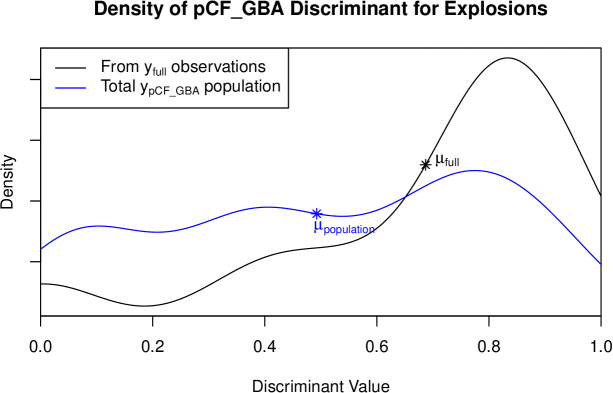
Figure 4: Density fits of subsets of the pCF_GBA discriminant recorded from explosions. The density fits are from the events for which the full $p=5$ discriminants were recorded (shown in black) and the total population of the pCF_GBA data discriminant for explosions (shown in blue). The mean values, noted as $\mu$, were taken after the logit transform and transformed back to $[0,1]$ for plotting.

Missing entries within the dataset do not appear to be missing at random. Fig. 4 illustrates this property with p-values computed from the signal complexity factors computed from explosions at the GBA array (written as pCF_GBA). Density fits of this discriminant from the total population and the subset of the data that is associated with full $p=5$ observations show that, for this case, the mean of the data taken from full $p=5$ observations is shifted significantly from the population mean. This implies that the distributions of values obtained from events with different degrees of data “missingness” may not be the same.

The experiment consisted of 250 MC iterations. Subsets of the data were sampled without replacement for training and testing, for each iteration. Because there were only two deep earthquake observations with full observations, and because the functions used for C-ECM require at least two full observations for each category, both of these observations were included in every training data set. The 18 additional full observations were randomly sampled from the data set to include in the training data. Of the remaining 255 partial observations, we used $\left\lfloor{255\times\sqrt{p}/(1+\sqrt{p})}\right\rfloor=176$ [33] for training. We used the remaining 84 observations, 79 partial observations and 5 full observations for testing.

The distribution of the observed model accuracy over each MC iteration is shown as box plots in Fig. 5. There is relatively less variability in the results from this real data set compared to Fig. 3. Median accuracy of M-B-ECM, M-B-ECM $C_{1,2}=2$, and M-B-ECM Cat is clearly better than that of C-ECM and B-ECM. If discriminants are not missing at random, the methods which utilize partial observations for training can get a better representation of the mean of the population, useful for predicting the category of $\tilde{\bm{y}}_{\tilde{p}}$ for testing data where $\tilde{p}\in\{1,\dots,5\}$.

The results of the total accuracy, false negative rate, and false positive rate calculated over the entirety of data collected are shown in Table 2. Results largely echo those in Table 1. B-ECM has slightly higher overall accuracy than C-ECM for this moderate $p=5$ problem. C-ECM has a much higher false negative rate than all B-ECM comparators and a lower false positive rate.

Including missing data to train a M-B-ECM model generally resulted in improved accuracy, a greatly reduced false negative rate, and a worse false positive rate. For many of the explosion discriminants, the population has a higher variance than the portion which is part of a full $\tilde{p}=5$ event. We hypothesize that the increase in variance for these discriminants within the training data translated to more true explosion $\tilde{\bm{y}}_{\tilde{p}}$ being captured as being more probable. The deep earthquake and shallow earthquake discriminant populations often have a lower variance than their explosion counterparts. Conversely, this increase in variance could also lead to more $\tilde{\bm{y}}_{\tilde{p}}$ which are not truly explosions to be categorized as such.

M-B-ECM $C_{1,2}=2$ resulted in a further reduction in the false negative rate, with little trade off in overall accuracy. Similar to what can be noted from Table 1, the lower threshold for categorization as an explosion results in a lower false negative rate and higher false positive rate than binary categorization with M-B-ECM and 0-1 loss.

Table 2: Empirical results from seismic discriminant experiments. Values in parenthesis are the difference observed from C-ECM, and are colored according to the magnitude of the difference as well as the benefit observed by utilizing the specific B-ECM implementation over C-ECM.

	$p$ = 5
C-ECM
Accuracy	0.71
False Negative	0.51
False Positive	0.01
B-ECM
Accuracy	0.75 ($\Delta$0.04)
False Negative	0.41 ($\Delta$-0.09)
False Positive	0.03 ($\Delta$0.02)
M-B-ECM
Accuracy	0.85 1 ($\Delta$0.14)
False Negative	0.12 ($\Delta$-0.39)
False Positive	0.18 ($\Delta$0.17)
M-B-ECM $C_{1,2}=2$
Accuracy	0.85 ($\Delta$0.14)
False Negative	0.09 ($\Delta$-0.42)
False Positive	0.24 ($\Delta$0.22)
M-B-ECM Cat
Accuracy	0.79 ($\Delta$0.08)
False Negative	0.1 ($\Delta$-0.41)
False Positive	0.21 ($\Delta$0.2)

Figure 5: Box plots showing the distribution of observed accuracy over the MC iterations for the seismic discriminant data set.

5 Discussion and Conclusions

Results consistently suggest that a B-ECM model trained on observations with no missing data has accuracy similar to or greater than a C-ECM model, as well as a lower false negative rate. The inclusion of additional training events where some data is missing for a B-ECM model consistently results in clear improvements in categorization accuracy and reductions in false negative rate over C-ECM. These findings indicate that B-ECM is a worthy competitor for event identification in operational treaty monitoring. The experiments in Sections 4.1 and 4.2 highlight these differences in performance. While C-ECM has relatively low false positive rates for all data used and all sizes of $p$ tested, B-ECM typically performs better in all other aspects for these difficult problems, and has a similar false positive rate for some problems. Adjusting the values of the loss matrix for applications where a lower false positive rate is desirable facilitates such a reduction if desired.

A B-ECM model which can handle training data with missing elements, assumes the data is missing completely at random. A combination of intuition and the evidence displayed in Fig. 4 leads us to believe missing data elements are not truly random. An intuitive hypothetical would be a low yield weapon not meeting certain thresholds in order to start automated data recording, resulting in some missing data for such an event. However, even with this nuanced model misspecification, simply having the ability to utilize data with missing entries results in significant performance gains. We expect further improvements in performance for a B-ECM model which instead has a missing not at random [38] specification.

The decision theoretic framework for B-ECM provides intuition to tune “knobs”, by changing values within the loss matrix, as in Equation (7). Values within the loss matrix could be chosen subjectively, as is done in Section 4, or tuned empirically given a large enough data set, in order to target a reduction in false negatives or false positives. When we increase the value of element $C_{1,2}$, logically we are increasing the loss associated with erroneously choosing to categorize $\tilde{\bm{y}}_{\tilde{p}}$ as not a detonation when the event truly is a detonation. The intuitive relationship between the values of the elements of a loss matrix has utility in operations. Just as important, changing the values of the loss matrix impacts the results as intended. In our experiments, increasing $C_{1,2}$ to a value of 2 in order to reduce the false negative rate did result in the intended reduction by roughly a factor of two, with only slight reductions in overall accuracy.

The B-ECM model is flexible enough to adapt to both detection and categorization applications. Sets of elements from the $K$ length vector from the predictive category distribution $p(\tilde{\bm{z}}_{K}|\tilde{\bm{y}}_{\tilde{p}},\bm{Y}_{N\times p},\bm{\theta})$ can be summed to group event categories together, so that B-ECM can be used to categorize $\tilde{\bm{y}}_{\tilde{p}}$ into anywhere from 2 to $K$ groups with a corresponding adjustment of the loss matrix. A larger number of actions to choose from corresponds with a decrease in accuracy. This increase in the complexity of the problem results in the observed decrease in accuracy for both data sets explored in experimentation. However, this effect appears to diminish as $p$ increases, which we hypothesize is due to a decrease in the overlap of $p(\tilde{\bm{y}}_{\tilde{p}}|\tilde{z}_{k}=1,\bm{Y}_{N_{k}\times p},\bm{\theta}_{k})$ in higher dimension for all $k$ Our testing with event categorization utilizes data with missing entries. Even though the categorization problem is more difficult, at times event categorization had higher accuracy than methods which did not take advantage of missing data. This was particularly true in Section 4.2. These results illustrate how powerful utilizing all data can be for more difficult problems.

We introduced a novel decision framework for the Bayesian typicality index, which is able to detect outliers under the uncertainty imparted by using partial data observations. The use of the Bayesian typicality index ensures that a $\tilde{\bm{y}}_{\tilde{p}}$ which was not generated from one of the $K$ events has the possibility of being categorized as an outlier. Without the typicality index, a new observation would be required to be categorized under the finite set of event categories used for training. The Bayesian typicality index is a B-ECM model specific twist on established methodology, which can take into account uncertainty related to using training data with missing entries.

With the ability to handle partial observations and the use of Bayesian Decision theory, B-ECM has been shown to be an improvement over C-ECM, and there are many avenues for continuing improvement even further over the current state of the art. Values of the matrix $\bm{C}$ and typicality index significance level $\tilde{\alpha}$ can be tuned to meet an application specific objective. The utility of loss matrices where the elements are functions instead of constants can be investigated [46, 8]. We believe taking advantage of Bayesian model selection procedures would produce further improvements in accuracy, especially in applications where data is fused over multiple modalities. In a preliminary investigation, we did not see consistent improvements in accuracy for the the logit function over the transform used in [3]. The preferable transform depends on the data itself, and the data can inform which transform to use as part of a Bayesian model selection procedure using Bayes Factors [35]. Additionally, model selection procedures can be used to allow uniquely sparse covariance matrices [32, 48] for each category and models which assume missing data is not at random [38]. For event categories where there is no correlation between particular discriminants, such a model may be a better fit to the data.

Author Contribution Statement

• Scott Koermer: Conceptualization, Formal analysis, Investigation, Methodology, Software, Validation, Visualization, Writing - original draft, Writing - review & editing

• Joshua D. Carmichael: Data curation, Supervision, Methodology, Visualization, Writing - original draft, Writing - review & editing

• Brian J. Williams: Methodology, Supervision, Writing - original draft, Writing - review & editing

Appendix A Nomenclature

References

- [1] Dale N Anderson “Sources of error: regional amplitude and teleseismic magnitude discriminants” In Monitoring Research Review: Ground-Based Nuclear Explosion Monitoring Technologies, 2009
- [2] Dale N Anderson and Steven R Taylor “Rediscovering signal complexity as a teleseismic discriminant” In Pure and Applied Geophysics 166.LA-UR-08-06754; LA-UR-08-6754 Los Alamos National Laboratory (LANL), Los Alamos, NM (United States), 2008
- [3] Dale N Anderson et al. “A mathematical statistics formulation of the teleseismic explosion identification problem with multiple discriminants” In Bulletin of the Seismological Society of America 97.5 Seismological Society of America, 2007, pp. 1730–1741
- [4] Dale N Anderson et al. “Seismic event identification” In Wiley Interdisciplinary Reviews: Computational Statistics 2.4 Wiley Online Library, 2010, pp. 414–432
- [5] Dale N Anderson, Robert H Shumway, Robert R Blandford and Steven R Taylor “Statistical methods in seismology” In Wiley Interdisciplinary Reviews: Computational Statistics 2.3 Wiley Online Library, 2010, pp. 303–316
- [6] DN Anderson et al. “Sources of error and the statistical formulation of Ms: mb seismic event screening analysis” In Pure and Applied Geophysics 171 Springer, 2014, pp. 537–547
- [7] Stephen J Arrowsmith and Steven R Taylor “Multivariate acoustic detection of small explosions using Fisher’s combined probability test” In The Journal of the Acoustical Society of America 133.3 AIP Publishing, 2013, pp. EL168–EL173
- [8] James O Berger “Statistical decision theory and Bayesian analysis” Springer Science & Business Media, 2013
- [9] Aaron Booker and Walter Mitronovas “An application of statistical discrimination to classify seismic events” In Bulletin of the Seismological Society of America 54.3 The Seismological Society of America, 1964, pp. 961–971
- [10] David Bowers and Neil D Selby “Forensic seismology and the comprehensive nuclear-test-ban treaty” In Annual Review of Earth and Planetary Sciences 37 Annual Reviews, 2009, pp. 209–236
- [11] Joshua Carmichael, Robert Nemzek, Neill Symons and Mike Begnaud “A method to fuse multiphysics waveforms and improve predictive explosion detection: theory, experiment and performance” In Geophysical Journal International 222.2 Oxford University Press, 2020, pp. 1195–1212
- [12] Joshua D Carmichael, Robert Nemzek, Stephen Arrowsmith and Kari Sentz “Fusing geophysical signatures of locally recorded surface explosions to improve blast detection” In Geophysical Journal International 204.3 Oxford University Press, 2016, pp. 1838–1842
- [13] George Casella and Edward I George “Explaining the Gibbs sampler” In The American Statistician 46.3 Taylor & Francis, 1992, pp. 167–174
- [14] Ola Dahlman and Hans Israelson “Monitoring underground nuclear explosions” Elsevier, 2016
- [15] Eva Elvers “Seismic event identification by negative evidence” In Bulletin of the Seismological Society of America 64.6 The Seismological Society of America, 1974, pp. 1671–1683
- [16] Ulf A Ericsson “Event identification for test ban control” In Bulletin of the Seismological Society of America 60.5 The Seismological Society of America, 1970, pp. 1521–1546
- [17] Donat Fah and Karl Koch “Discrimination between earthquakes and chemical explosions by multivariate statistical analysis: A case study for Switzerland” In Bulletin of the Seismological Society of America 92.5 Seismological Society of America, 2002, pp. 1795–1805
- [18] Sean R Ford et al. “Joint Bayesian inference for near-surface explosion yield and height-of-burst” In Journal of Geophysical Research: Solid Earth 126.2 Wiley Online Library, 2021, pp. e2020JB020968
- [19] Sean R Ford et al. “Joint Bayesian inference for near-surface explosion yield and height-of-burst” In Journal of Geophysical Research: Solid Earth 126.2 Wiley Online Library, 2021, pp. e2020JB020968
- [20] Sean R Ford et al. “Partitioning of seismoacoustic energy and estimation of yield and height-of-burst/depth-of-burial for near-surface explosions” In Bulletin of the Seismological Society of America 104.2 Seismological Society of America, 2014, pp. 608–623
- [21] Jerome H Friedman “Regularized discriminant analysis” In Journal of the American statistical association 84.405 Taylor & Francis, 1989, pp. 165–175
- [22] Alan E Gelfand and Adrian FM Smith “Sampling-based approaches to calculating marginal densities” In Journal of the American statistical association 85.410 Taylor & Francis, 1990, pp. 398–409
- [23] Alan E Gelfand, Susan E Hills, Amy Racine-Poon and Adrian FM Smith “Illustration of Bayesian inference in normal data models using Gibbs sampling” In Journal of the American Statistical Association 85.412 Taylor & Francis, 1990, pp. 972–985
- [24] Andrew Gelman, John B Carlin, Hal S Stern and Donald B Rubin “Bayesian data analysis” ChapmanHall/CRC, 1995
- [25] Stuart Geman and Donald Geman “Stochastic relaxation, Gibbs distributions, and the Bayesian restoration of images” In IEEE Transactions on pattern analysis and machine intelligence IEEE, 1984, pp. 721–741
- [26] David N Green et al. “Hydroacoustic, infrasonic and seismic monitoring of the submarine eruptive activity and sub-aerial plume generation at South Sarigan, May 2010” In Journal of Volcanology and Geothermal Research 257 Elsevier, 2013, pp. 31–43
- [27] Arjun K Gupta and Daya K Nagar “Matrix variate distributions” ChapmanHall/CRC, 2018
- [28] David A Harville “Matrix algebra from a statistician’s perspective” Taylor & Francis, 1998
- [29] Stephen Herzog “The nuclear test ban: Technical opportunities for the new administration” In Arms Control Today 47.1 JSTOR, 2017, pp. 26–32
- [30] Peter D Hoff “A first course in Bayesian statistical methods” Springer, 2009
- [31] Ron-Song Jih et al. “Magnitude: Yield Relationship at Various Nuclear Test Sites–A Maximum-Likelihood Approach Using Heavily Censored Explosive Yields”, 1990
- [32] Michael Irwin Jordan “Learning in graphical models” MIT press, 1999
- [33] V Roshan Joseph “Optimal ratio for data splitting” In Statistical Analysis and Data Mining: The ASA Data Science Journal 15.4 Wiley Online Library, 2022, pp. 531–538
- [34] Martin B Kalinowski et al. “Innovation in Technology and Scientific Methods for Nuclear Explosion Monitoring and Verification: Introduction” In Pure and Applied Geophysics 180.4 Springer, 2023, pp. 1227–1234
- [35] Robert E Kass and Adrian E Raftery “Bayes factors” In Journal of the american statistical association 90.430 Taylor & Francis, 1995, pp. 773–795
- [36] Keith D Koper “The importance of regional seismic networks in monitoring Nuclear Test-Ban Treaties” In Seismological Research Letters 91.2A GeoScienceWorld, 2020, pp. 573–580
- [37] Samuel Kotz and Saralees Nadarajah “Multivariate t-distributions and their applications” Cambridge University Press, 2004
- [38] Roderick JA Little and Donald B Rubin “Statistical analysis with missing data” John Wiley & Sons, 2019
- [39] Monica Maceira et al. “Trends in Nuclear Explosion Monitoring Research & Development - A Physics Perspective -” Sponsor: USDOE, 2017 URL: http://permalink.lanl.gov/object/tr?what=info:lanl-repo/lareport/LA-UR-17-21274
- [40] Kaegan McGrath “Verifiability, Reliability, and National Security: The Case for US Ratification of the CTBT” In Nonproliferation Review 16.3 Taylor & Francis, 2009, pp. 407–433
- [41] Geoffrey J McLachlan “Discriminant analysis and statistical pattern recognition” John Wiley & Sons, 2005
- [42] Henry R Myers “Comprehensive Test Ban Treaty: Grounds for Objection Diminish” In Science 175.4019 American Association for the Advancement of Science, 1972, pp. 283–286
- [43] Kai Wang Ng, Guo-Liang Tian and Man-Lai Tang “Dirichlet and related distributions: Theory, methods and applications” John Wiley & Sons, 2011
- [44] Brian J Redman et al. “Hyperspectral vegetation identification at a legacy underground nuclear explosion test site” In Chemical, Biological, Radiological, Nuclear, and Explosives (CBRNE) Sensing XX 11010, 2019, pp. 145–154 SPIE
- [45] Christian P Robert and George Casella “Monte Carlo statistical methods” Springer, 1999
- [46] Christian P Robert “The Bayesian choice: from decision-theoretic foundations to computational implementation” Springer, 2007
- [47] Rebecca L Rodd et al. “A Multimodal Event Catalog and Waveform Data Set That Supports Explosion Monitoring from Nevada, USA” In Bulletin of the Seismological Society of America Seismological Society of America, 2023
- [48] Alberto Roverato “Hyper inverse Wishart distribution for non-decomposable graphs and its application to Bayesian inference for Gaussian graphical models” In Scandinavian Journal of Statistics 29.3 Wiley Online Library, 2002, pp. 391–411
- [49] Sarah Scoles “A model to detect explosions big and small”, 2020
- [50] RH Shumway, DW Rivers and TELEDYNE GEOTECH ALEXANDRIA VA ALEXANDRIA LABS “Testing the Hypothesis of TTBT (Threshold Test Ban Treaty) Compliance, and Magnitude-Yield Regression for Explosions in Granite”, 1984
- [51] Robert H Shumway “Classical and Bayesian seismic yield estimation: The 1998 Indian and Pakistani tests” In pure and applied geophysics 158 Springer, 2001, pp. 2275–2290
- [52] Robert H Shumway “Statistical approaches to seismic discrimination” In Monitoring a comprehensive test ban treaty Springer, 1996, pp. 791–803
- [53] Matthew Stephens and D Phil “Bayesian methods for mixtures of normal distributions”, 1997
- [54] Steven R Taylor, Stephen J Arrowsmith and Dale N Anderson “Detection of short time transients from spectrograms using scan statistics” In Bulletin of the seismological society of America 100.5A Seismological Society of America, 2010, pp. 1940–1951
- [55] S Ulam and Nicholas Metropolis “The Monte Carlo Method” In Journal of the American Statistical Association 44.245 Washington: American Statistical Association, 1949, pp. 335
- [56] Claus Weihs, Uwe Ligges, Karsten Luebke and Nils Raabe “klaR Analyzing German Business Cycles” In Data Analysis and Decision Support Berlin: Springer-Verlag, 2005, pp. 335–343
- [57] Brian J Williams et al. “Multiphenomenology explosion monitoring (MultiPEM): a general framework for data interpretation and yield estimation” In Geophysical Journal International 226.1 Oxford University Press, 2021, pp. 14–32
- [58] Ruoyong Yang and James O Berger “A catalog of noninformative priors” Institute of StatisticsDecision Sciences, Duke University Durham, NC, USA, 1996