Statistical analysis on the effectiveness of a low insulin index, alkaline and functional diet evaluated with machine learning techniques

Abstract

In this paper, a statistical analysis of the performance of a low insulin index, alkaline and functional diet developed by ANTUR evaluated with machine learning techniques is reported. The sample of patients was checked on a regular basis with a BioImpedenziometric (BIA) analysis. The BIA gives about 40 parameters output describing the health status of the patient. The sample of 1626 patients was grouped in clusters with similar characteristics by a neural network algorithm. A study of the behaviour of the BIA parameters evolution over time with respect to the first visit was performed. More than the 75% of the patient that followed the ANTUR diet showed an improvement of the health status.

Keywords Machine learning  $\cdot$ Nutrition Science  $\cdot$ Artificial Neural Network

1 Introduction

In recent decades, according to World Health Organization, the incidence of overweight and obesity in the population has been one of the most serious public health problems in Western countries. Obesity is one of the major risk factors underlying of the premature onset of cardiovascular and cerebrovascular diseases, diabetes, osteoporosis, gastrointestinal diseases and some cancers [1].

2 Antur Diet: a low insulin index, alkaline and functional diet

The main goal of the Antur diet is to improve patient well-being and reduce body weight by primarily targeting fat mass. Patients were given a low-insulin, alkaline, and functional diet, which was proposed as a useful tool in the prevention of silent inflammation and chronic diseases, as well as in the management of established diseases. The Antur diet aims to be a low-insulin diet, as hyperinsulinemia is associated with overweight [2], alterations in glucose metabolism, poor lipid profile [3, 4], hypertension [5], increased risk of early-onset prostate cancer [6], and insulin resistance, a condition typical of various diseases, such as type 2 diabetes mellitus [7] and polycystic ovary syndrome [2]. In order to ensure the proper functioning of physiological processes, blood pH should be between 7.35 and 7.45 [8]. Values below 7.35 lead to acidosis, which predisposes to various disorders, including vasodilation, insulin resistance, reduction in neuronal excitability, impairment of the immune system [8], and bone demineralization [9, 10]. The condition of acidosis is due to an unbalanced diet, renal diseases, diabetes, medication consumption, altered renal acid excretion, mineral loss, altered lactate metabolism, and tumors [11, 12]. The alkaline diet is based on the intake of alkaline foods, negative potential renal acid load (pral) index, that counteract the acidifying effect of positive pral index foods, in order to have an overall alkaline balance and counteract any decreases in pH. The Antur diet is based on the use of foods, considering not only their calories and macro-nutrient content, but also their micro-nutrient content, as these exert (positive or negative) effects in various body areas. The cooking method is also fundamental [13], as it must be able to preserve the benefits of the foods without sacrificing taste. Functional nutrition can be a valuable support in the management of various diseases, such as type 2 diabetes mellitus [14], and in limiting the impact of the side effects associated with drug intake [15]. Fundamental components of the functional diet are spices and herbs for their antioxidant, digestive, lipid- lowering, antibacterial, anti-inflammatory, antiviral, and anticancer properties [16].

Patients followed nutritional plans with the above-mentioned characteristics, but personalized according to their own needs, preferences, the possible presence of diseases and/or food allergies/intolerances, and based on their body weight. Each nutritional plan involved the alternation of three phases cyclically repeated until the goal was reached.

• Phase 1 - non-alkaline attack phase in which the patient consumed:

  • 1.3 g/kg of body weight of protein

  • 0.7 g/kg of body weight of carbohydrates

  • 1.2 g/kg of body weight of lipids

• Phase 2 - functional and low-insulin index phase in which the patient consumed:

  • 1.2 g/kg of body weight of protein

  • 1.5 g/kg of body weight of carbohydrates

  • 1.0 g/kg of body weight of lipids

• Phase 3 - alkaline and functional phase in which the patient consumed:

  • 1.0 g/kg of body weight of protein

  • 1.3 g/kg of body weight of carbohydrates

  • 0.9 g/kg of body weight of lipids

3 Data taking with the BIA machine

Body weight divided by the square of the height results in Body Mass Index (BMI), which lead to establish whether an individual is underweight, normal weight, overweight or obese. However, BMI does not describe body composition neither hydration status. Bioimpedance analysis (BIA) is a doubly indirect method to assess body composition. BIA is a safe, non-invasive and cost-effective test; it provides quick and reproducible results and the equipment to perform the exam is easily transported. Therefore, BIA is also used in hospital to monitor the nutritional and hydration status of hospitalized patients. In this method, body consists in an electrical circuit in which two or more resistors and capacitors are connected in parallel [17]. BIA allows to quantify total body water (TBW) by measuring body impedance. The interest in the application of bioelectric impedance to human body has developed from the first studies on the relationship between the bioelectric impedance and the content of body water and physiological variables in human and animal tissues. Impedance ($\hat{Z}$) is the frequency-dependent opposition of a conductor to the flow of an alternating electric current. It is a complex quantity, since $\hat{Z}\in\mathcal{C}$, and thus can be defined by its module $Z$ and phase $\phi$. The impedance module can be derived from:

$$Z=\sqrt{R^{2}+X_{C}^{2}},$$ (1)

where $R$ is the resistance and $X_{C}$ is the reactance [18]. Body resistance is determined by:

$$R=\rho\frac{L}{A},$$ (2)

where $L$ is the shape/length and $A$ is the surface, and $\rho$ is the intrinsic resistivity area of the body. In biological systems, resistance is due to the presence of water. The reactance is the body property to resist voltage variations; it is inversely proportional to the signal frequency ($\omega$) and to the capacitance (C):

$$X_{C}=\frac{1}{\omega C}$$ (3)

In biological systems the reactance is due to the presence of cell membranes that work as capacitors consisting of two plates separated by an insulating layer that stores electric charges. The bioelectric impedance is more influenced by the resistance, because of the greater presence of water than membranes in human body. The phase angle can be derived from resistance and reactance, as:

$$\phi=\arctan\left(\frac{X_{C}}{R}\right)\frac{180^{\circ}}{\pi}$$ (4)

The phase angle represents the angle between the impedance vector and the resistance. The phase angle is directly proportional to the reactance; hence it is considered an indicator of cell integrity. This parameter is also widely used in hospital to predict the long-term survival of patients suffering from diseases like liver cirrhosis [19], pulmonary diseases [20], HIV infections [21] and AIDS [22], several types of cancer [23, 24], dialysis [25, 26], bacteremia [27] and sepsis [28]. The phase angle varies depending on age, sex and ethnicity [29]. This parameter increases as free-fat mass increases [30] and it decreases in inflammatory status, because cell membranes can be damaged when oxidative stress occurs [31] and in elderly subjects [32]. At low frequencies, electric current can only flow through body fluids, while at high frequencies it can penetrate through cell membranes. Due to wide amount of water and electrolytes, in the Free-Fat Mass (FFM) the observed impedance is slightly lower than measured impedance in Fat Mass [33]. Originally, BIA assessed body composition by measuring the impedance using a single 50 kHz frequency, generally detected between the wrist and the ankle, as suggested by Nyboer et al. his studies established that 50 kHz was the critical frequency of muscle tissue, hence the current frequency at which the reactance maximum is recorded [34]. According to the axioms of impedance plethysmography, the square of the height (the “length” of the “conductor”) divided by the total body resistance results in impedance index, which is a total conductive volume index. This index can describe the FFM volume, due to higher electrolyte content and higher conductivity of FFM compared to adipose tissue [35]. Impedance is mainly determined by resistance, which depends on the amount of tissue fluids; therefore the single-frequency bia (Sf-BIA) is able to determine the total body water and the lean mass that is 73% hydrated. Fat mass is calculated by the difference between body weight and lean mass [36]. In the 1960s Thomasset et al. established that it is possible to discriminate between intracellular and extracellular water by using different frequencies (both high and low frequencies); this allows a more accurate estimation of body composition [37]. At first human body was considered as a single cylindrical block with uniform cross-sectional area, but a better approximation describes the human body as a sum of five different cylinders (two upper limbs, two lower limbs and the trunk). In order to clarify how every body segment affects the total body impedance, Segmental BIA method was developed [38]. To estimate body composition, InBody 570 was used in this study. It uses the Direct Segmental Multifrequency Bioimpedance Analysis (DSM-BIA), an accurate and precise technology which allows a multi-frequency analysis for each body segment separately; therefore, impedance values are provided for each body district and for each frequency used. InBody 570 is equipped of eight tactile and fixed electrodes, allowing the electrical circuits to always maintain the same length which results in a high level of accuracy and reproducibility. In addition, InBody570 evaluate data derived from the measured impedance, avoiding empirical estimates; age and sex only define confidence intervals for each parameter [39].

4 Statistical description of the sample of patients

In this section a statistical description of the patients samples is given. The variables recorded for each patient and for each BIA test are 23 and they are categorised in 6 main groups: Hydration, Circumferences, Adiposity, Body Composition, Muscularity e Metabolism. As can be seen in Table 1, Hydration group contains ECW (Extra Cellular Water), TBW (Total Body Water) and ICW (Intra-Cellular Water) variables, the Circumferences group contains the dimension (in cm) of waist, neck, chest, hips, arm, thigh, the body composition group is formed by the BMI (Body Mass Index) and the WHR (Waist-to-Hip ratio), the Muscularity group is composed by SMI (Skeletal Muscle Index) and SMM (Skeletal Muscle Mass), the Adiposity group is composed by FFM, Visceral Fat Level (VFL), Body Fat Mass (BFM), Obesity degree variables, and Metabolic group which is formed by Body Cell Mass (BCM), Minerals, Protein, Basal Metabolic Rate (BMR).

Data
Hydration	Adiposity	Metabolism	Muscularity	Body Composition	Circumferences
Extra-Cellular Water (ECW)	Fat Free Mass (FFM)	Body Cell Mass (BCM)	Skeletal Muscle Index (SMI)	Body Mass Index (BMI)	Waist
Total Body Water (TBW)	Visceral Fat Level (VFL)	Minerals	Skeletal Muscle Mass (SMM)	Waist-to-Hip Ratio (WHR)	Neck
Intra-Cellular Water (ICW)	Body Fat Mass (BFM)	Protein			Chest
	Obesity Degree	Basal Metabolic Rate (BMR)			Hips
					Arm
					Thigh

Table 1: Summary table of the 6 groups of variables obtained from each BIA test.

Each patient after the first BIA test receives a prescription treatment protocol (ANTUR diet) to be followed in order to improve its health status. The protocol contains a diet, advice for physical activity and, more generally, for a healthier lifestyle. The data analysis presented here has the goal of studying the behaviour of the BIA variables, connected to the health status and the wellness of the patient, as a function of the time from the first BIA test.

The data samples of 9080 tests undergo a first cleaning by excluding the records with:

• a single BIA test;

• broken and/or incomplete registration data.

After the first cleaning-up, the data sample is composed by 1626 patients of which 424 are male and 1202 are female, as reported in Table 2. The total number of records (BIA tests performed on the patients’ sample) in 6 months is 6664.

	Male	Female	Total
Patients	424	1202	1626
Total BIA tests	1436	5520	6664

Table 2: Data sample information: analysis records divided by male and female.

4.1 Characterization of the data samples

Taking as reference values’ for the BMI the Tab. 3, the full sample of patients (1626 people), split in male and female and before the nutrition treatment start (trial 0), have the BMI distribution showed in pie charts in Figure 1.

Status	BMI
Underweight	<18.5
Normal weight	18.6-24.9
Overweight	25.0-29.9
Moderately obese	30.0-34.9
Severely obese	35.0-39.9
Very severely obese	>40

Table 3: BMI reference value.

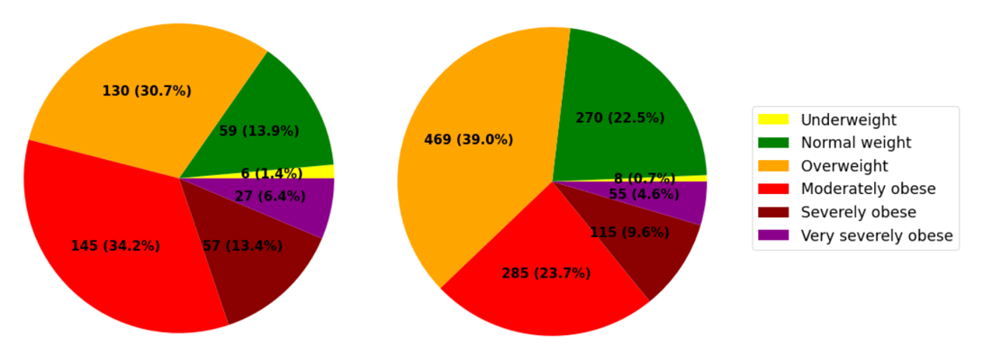
Figure 1: BMI distribution of the sample at the first BIA test (trial 0) for males (on the left) and for females (on the right).

About 15% of males (23% of females) are underweight/normal weight. They need a maintenance diet for the weight and to improve other biologic parameters for an improved wellness. The 31% (39%) are overweight, while the remaining 54% (38%) shows obesity of some level. This represents the starting point dataset on which the ANTUR nutrition treatment has been applied.

The BMI is a good indicator but it’s not the only relevant one. Another important parameter is the waist-to-hip ratio (WHR), commonly used as a marker of cardiovascular risk. Reference values for WHR are reported in Tab. 4.

Risk level	Male	Female
Low	$<0.80$	$<0.70$
Average	0.81-0.90	0.71-0.80
Increasing	0.91-0.99	0.81-0.89
High	1.00-1.19	0.90-1.09
Very high	1.20-1.29	1.10-1.19
Extremely high	$>1.30$	$>1.20$

Table 4: WHR reference value.

Before starting the ANTUR treatment, about 25% of males (and only 2% of females) shows low/average risk with respect to WHR thresholds. About 38% (26%) have an increasing risk, while the 37% (72%) shows a high/very high/extremely high risk, as reported in the pie charts in Figure 2.

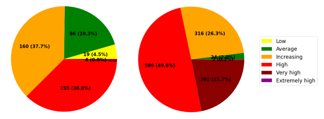
Figure 2: Weist-to-Hip ratio (WHR) sketch of the sample at the first BIA test (trial 0) for males (on the left) and for females (on the right).

Moreover to have a more detailed overview of the used dataset mean, standard deviation and percent error values for all the variables recorded at the first BIA test (trial 0) for all the patients are reported in table 5.

Variable:	Mean	Standard deviation	Percent error [%]
Circumference arm [cm]	34.81	5.46	16
Circumference neck [cm]	37.88	4.24	11
Circumference chest [cm]	100.74	9.94	10
Circumference waist [cm]	98.25	15.56	16
Circumference hip [cm]	103.37	8.85	9
Circumference right thigh [cm]	55.98	5.54	10
Gender [fraction of females]	0.74	0.44	59
Height [cm]	164.08	8.87	5
Age	38.38	14.98	39
Weight [kg]	79.76	18.59	23
ICW [%]	22.62	4.77	21
Proteins	9.78	2.06	21
Minerals	3.45	0.72	21
SLM	46.87	9.78	21
BMI [kg/m2]	29.49	5.75	20
PBF	36.71	8.87	24
FFM right arm	2.72	0.77	28
FFM left arm	2.69	0.76	28
FFM trunk	22.58	4.65	21
FFM right leg	7.51	1.72	23
FFM left leg	7.48	1.68	22
BFM right arm	2.52	1.73	69
BFM left arm	2.53	1.74	69
BFM tronco	15.03	5.60	37
BFM right leg	4.28	1.61	38
BFM left leg	4.26	1.59	37
Target weight [kg]	63.01	10.62	17
BMR	1444.03	223.61	15
WHR	0.95	0.08	9
VFL	13.27	5.06	38
Obesity degree	139.63	26.87	19
AMC	29.06	4.07	14
BMC	2.85	0.60	21
Circumference right arm [cm]	34.89	5.46	16
Circumference left arm [cm]	34.81	5.46	16
Circumference left thigh [cm]	55.64	5.26	9
SMI	7.48	1.10	15
Recommended calories [kcal]	2008.34	498.46	25
BFM [%]	36.70	8.88	24
FFM [%]	63.30	8.88	14
SMM	34.91	5.12	15
BCM	41.24	5.90	14
TBW	46.45	6.43	14
ECW [%]	61.45	1.95	3
Total number of patients	1626

Table 5: Mean, standard deviation and percent error values for all the variables recorded at the first BIA test for all the patients.

5 Machine learning to obtain clusters of patients

To evaluate the performance of the ANTUR approach a Self-organizing map has been developed to cluster patient with common characteristics. Self-organizing maps (SOMs) are a special type of artificial neural networks trained using unsupervised learning. They allow the data sample to be divided into classes with similar properties. The data sample is branched into a training, validation and test samples. The training sample is a subset of tge dataset used for the learning phase. Validation is a technique in machine learning to evaluate the performance of models during learning and the validation sample is a subset of examples used to tune the parameters of the network. The test sample is a subset of data not used in the learning phase used to evaluate the results of the developed network. The SOM network makes it possible to produce a representation of the data sample provided as input, generally high-dimensional, in a low-dimensional space while preserving its topological properties. This property makes SOMs particularly useful for visualizing high-dimensional data. The model was first described by Teuvo Kohonen, and it is often referred to it as Kohonen maps [40]. Self-organizing maps are laterally connected neural networks where output neurons are organized in low-dimensional (usually 2D or 3D) grids. Each input is connected to all output neurons, such that each output neuron j is associated with a weight vector $W_{j}$ of the same size as the inputs vector, as can be seen from Figure 3 where a schematic view of the network architecture is shown. The size of the input vector is generally high and the output used in this work is a 2D map.

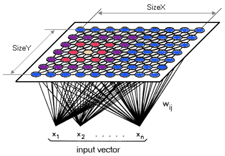
Figure 3: Schematic view of a SOM architecture. In most cases, n $\times$ the number of input variables is much bigger than the 2 dimensions associated to the output grid.

The goal of learning in SOMs is to specialize different parts of the grid to respond similarly to particular input patterns. This is inspired in part by how visual, auditory, or other sensory information are handled by separate parts of the cerebral cortex in the human brain. SOMs learn to classify the data provided as input to the network based on the identification of common features obtained by analyzing all the variables provided. Therefore, SOMs learn both distribution (as well as competitive levels) and the topology of the input vectors on which they are trained. The SOM networks are used for various applications, of which, one of the main ones, is clustering that is, the partitioning of a dataset into a collection of classes, or clusters, with similar characteristics. The way these networks train is through a competitive mechanism, where all of the output neurons take part in a "winner takes all" competition. The winner neuron j is the one having the maximum output value Y, defined as

$$Y_{j}=\sum_{i}w_{ij}*x_{i}$$ (5)

where $w_{ij}$ is the weight matrix of the network and $x_{i}$ is the inputs vector. This analytic relation shows that the chosen neuron is also the one for which the weight vector $W_{j}$ is the most similar to $x_{i}$. Once the winner is established, the weight vectors are updated only for this neuron and for those belonging to its neighbourhood (active neurons), defined by an ad hoc neighbouring function H. The difference depends on the distance from the winning neuron, so that weights associated to farthest neurons are changed less than the closest ones [41]. Through this mechanism, groups of neurons with similar properties are created. The training process is interrupted when the SOM output stops changing or no significant changes are observed.

This type of network is particularly indicated when working with a not homogeneous sample, like the one described in Sec. 4 and used in this work. A SOM network is applied to the dataset of the patients by dividing the sample in training, and test with a ratio of 66:34. The parameters of the network applied are:

• $5\times 4$ grid topology: 20 neurons

• Euclidean distance metric

• weights modification occurs within a maximum range of three nodes

• 5000 training epochs

• 18 input variables.

Figure 4 shows the grid topology of the SOM network used (on the left) and the cluster definition performed after the training (on the right).

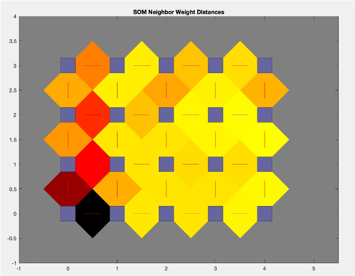
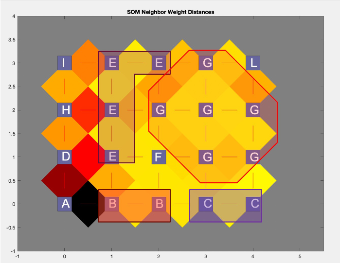
Figure 4: Output of the SOM network (on the left) and sketch of the definition of the cluster (on the right). Clusters here are labelled with letters from A to L, while in the following sections they will be labelled with numbers from 1 to 10.

In this figure, the squares represent the output neurons connected by red lines, while the color indicate the distance between them: a lighter color (yellow) is associated with a short distance, whether a darker color (red-black) is associated with a larger distance. Here, the distance is the euclidean distance in the $x-y$ plane. By looking for regions in the grid with yellow color enclosed in red colored segment strips, 10 clusters were identified labelled with letters from A to L. In the following paragraphs, they will be referred to with numbers from 1 to 10.
Moreover, in Figure 5, the hit maps for males, females and both kinds of patients are reported. In these, again, each square is an output neuron, and the numbers represent how many data features among the totality of network inputs are associated to each neuron. They show that the clusters not only present a remarkable difference between each other in their unique characteristics, but we can also see that some clusters, hence some characteristics, are mostly associated to males (upper-left region) while others are mostly associated to females (lower-right region).

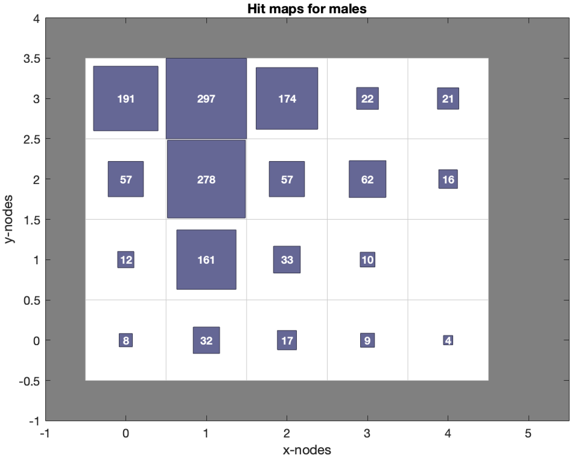
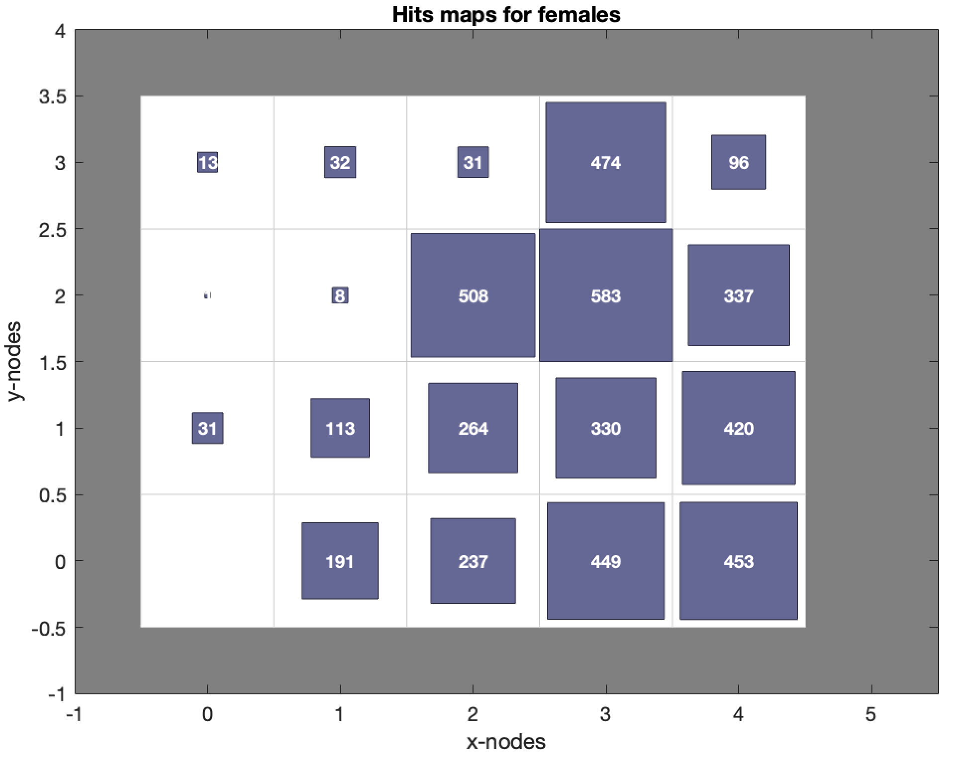
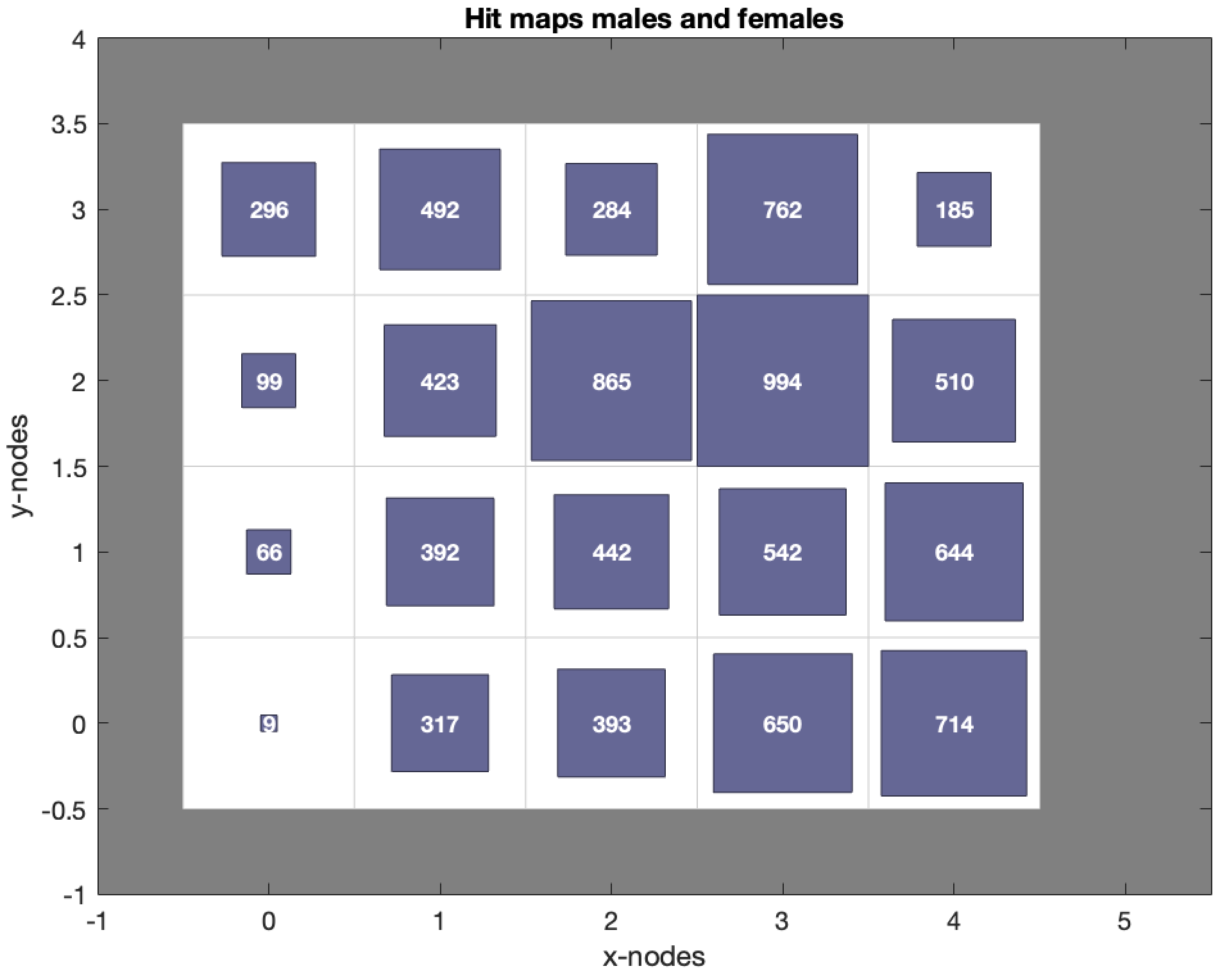
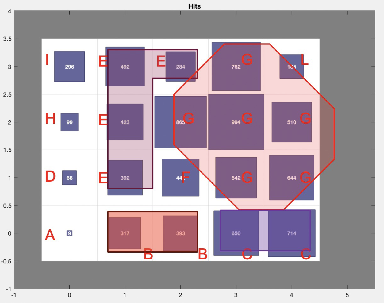
Figure 5: Hit maps for males (upper left) and females (upper right) in the training dataset. The lower hit maps are for the total number of patients (left) and the same with the superimposed cluster definition (right).

6 Statistical description of the ML clusters

A total of 10 clusters are defined according to the SOM network defined in Sec. 5. The cluster defined are characterized by analyzing the features used to train the SOM network and Table 6 reports the features mean values for the first BIA test.

Mean value for the cluster:	1	2	3	4	5	6	7	8	9	10
Gender [fraction of females]	0.00	0.89	0.99	0.62	0.21	0.90	0.94	0.04	0.08	0.65
Age	41.50	44.39	55.00	39.16	38.52	27.11	34.57	38.09	36.06	22.90
Height [cm]	182.00	160.98	157.63	164.00	173.83	161.23	161.49	179.12	178.45	152.26
Weight [kg]	184.50	100.60	76.14	129.14	86.60	87.31	67.96	133.15	109.92	43.54
BMI [kg/m2]	55.80	38.83	30.66	48.07	28.72	33.62	26.04	41.45	34.56	18.82
BFM [%]	50.30	49.15	43.38	52.20	28.63	45.51	34.44	42.26	36.76	20.54
FFM [%]	49.70	50.85	56.62	47.80	71.37	54.49	65.56	57.74	63.24	79.46
Neck circumference [cm]	50.30	44.47	37.96	50.59	38.93	40.27	35.03	46.77	42.69	29.24
Chest circumference [cm]	130.30	113.87	100.04	126.27	104.99	105.87	93.92	123.75	115.22	78.22
Waist circumference [cm]	153.53	119.84	100.17	134.27	99.17	107.73	88.40	137.94	120.62	66.56
Hip circumference [cm]	141.35	115.71	102.94	128.84	104.86	109.35	97.86	123.68	114.55	84.54
Right arm circumference [cm]	82.88	42.41	34.99	52.13	35.29	37.58	31.74	46.70	39.89	24.72
Left arm circumference [cm]	83.25	42.26	34.90	52.06	35.20	37.52	31.69	46.51	39.88	24.64
Right thigh circumference [cm]	73.23	62.12	54.78	68.74	57.45	60.05	52.99	67.18	63.09	44.62
Left thigh circumference [cm]	69.95	61.56	54.55	66.93	57.12	59.49	52.77	65.87	62.53	44.60
Total number of patients	4	136	224	16	300	107	707	24	73	34

Table 6: Mean values of the most important BIA variables at the first visit for patients belonging to the 10 clusters, as categorized by the SOM network outcome.

By referring to Tab. 6 one can notice that:

• cluster 1 is exclusively characterized by males with a very high BMI;

• cluster 2 is largely characterized by medium-aged females with a quite high BMI;

• cluster 3 is almost exclusively characterized by medium-aged females with a high BMI;

• cluster 4 is largely characterized by males and females with a very high BMI;

• cluster 5 is mainly characterized by males with a BMI slightly above average;

• cluster 6 is largely characterized by young females with a high BMI;

• cluster 7 is largely characterized by females with a BMI slightly above average;

• cluster 8 is mainly characterized by males with a medium-high BMI;

• cluster 9 is largely characterized by young males with a high BMI;

• cluster 10 is mainly characterized by very young males and females with a BMI slightly below average.

All patients adhered to the functional low-insulin diet prescribed by the ANTUR society, but their specific goals varied depending on their assigned cluster. For instance, patients in clusters 1 or 4 aimed to reduce their BMI, regulate the proportion of FFM and BFM, and improve hydration. Conversely, patients in cluster 10 sought to increase their BMI and FFM. Despite the disparate objectives, the functional low-insulin diet can be tailored to meet diverse requirements.

The aim of this project is to conduct a statistical analysis of biological parameters measured through bioelectrical impedance analysis (BIA). The analysis will follow the Knowledge Discovery in Databases (KDD) [42] process to uncover new insights from the data. The main strategy is to develop a model that can describe how the BIA parameters change over time since the start of the ANTUR treatment.

The initial step involved reporting biological parameters for each patient as a function of the elapsed time since their first visit. Next, a linear model was introduced to capture the temporal trend, which can be expressed as:

$$y=a+bx,$$ (6)

where $y$ represents the biological variable under investigation, $x$ denotes the time interval from the first visit, $b$ indicates the variation of the biological variable over time, and $a$ represents the initial value of the biological variable.

Since these two parameters are unknown, a least squares procedure is performed to determine their values. This procedure identifies the best-fit straight line that describes the patient’s data. The obtained parameters are interpreted as follows:

• $a$ is the starting value of the biological variable at the beginning of treatment, as predicted by the statistical inference.

• $b$ represents the daily rate of variation of the BIA parameter, which can be easily translated into the monthly variation rate.

6.1 Time behavior of the main BIA parameters

This study analyzed the relationship between the biological variables and the elapsed time from the start of the nutritional treatment to understand the variation of biological variables with time and to assess the effectiveness of the dietary protocol. The main focus was on the following six sectors:

• Body composition and cardiovascular disease risk

• Hydration

• Adiposity

• Muscularity

• Circumferences (neck, waist, thigh, etc)

• Target weight.

As example, in Figure 6, the BMI of a male patient with a 2^nd degree obesity belonging to the cluster 1. The vertical axis is the BMI (expressed in kg/m²), while on the horizontal axis the elapsed time from the beginning of the nutritional treatment is reported. This patient started with a very high BMI of 36.8 kg/m² and after 5 months of treatment it decreased to 33.5 (a decrease of 9%). The plot shows that the BMI decreases linearly with time, which was observed overall for every patient in similar conditions. The data points of BMI values at different medical trials were fitted with a linear model using equation:

$$\mathrm{BMI_{t}}=\mathrm{BMI_{0}}+b\cdot t,$$ (7)

where BMI₀ is the BMI value at the beginning of the treatment, $t$ is the time elapsed from the first medical trial, BMI_t is the BMI value at a given time $t$, while $b$ is the slope of the straight line representing the $\Delta$BMI/day. For this patient, the resulting slope value is $b=-0.021$ BMI/days, indicating a consistent improvement of -0.6 BMI points per month over 5 months of treatment. If the trend continues, the patient would reach the status of "Overweight" in 10 months and "Normal weight" in 18 months.

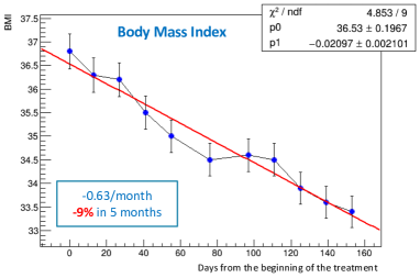
Figure 6: Time dependence of the BMI (kg/m²) for the patient ID1556.

A similar analysis has been performed for the WHR as a function of time. As depicted in Fig. 6, the patient started the treatment ranked as "high risk" (WHR$=1.05$) for cardiovascular disease. After 5 months of treatment, its WHR decreased to 0.97 (8% reduction), ranked as "Increasing risk". It is clear from the plot that also WHR decreases linearly with time during the treatment. Thus, we performed a linear fit with the equation:

$$\mathrm{WHR_{t}}=\mathrm{WHR_{0}}+c\cdot T,$$ (8)

where WHR₀ is the WHR value at the beginning of the treatment, $T$ is the time elapsed from the first medical trial, WHR_t is the WHR value at a given time $t$, while $c$ is the slope of the line and it represents the $\Delta$ WHR/day. In this particular case, the resulting value of the fit slope is $c=-4.6\cdot 10^{-4}$ WHR/day. This indicates that the patient got a constant improvement of about -0.014 WHR points per month, over 5 months of treatment. If the trend stays constant one can foresee that the patient in 10 months would be ranked "In Average" while after 18 months he would be ranked "Low risk".

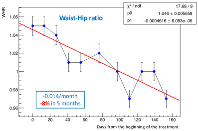
Figure 7: Time dependence of the WHR for the patient ID1556.

For what concerns the Body Adiposity, a study of the trends of the obesity degree and of the visceral fat level (VFL) have been performed. In Figure 8 the data points and the trend lines for both obesity degree and VFL are reported. Also in this case, both the variables follow a linear trend with a 10% reduction for the obesity degree and a 25% reduction fot the VFL. In particular, the patient with ID 1556 was able to reduce the VFL from 20, classified as "very high" as reported in Table 7, down to 16 in 5 months. In 2 additional months, if the behaviour continues, the patient will decrease the VFL classification level from "very high" to "high" and in 7 more months will reach the status "normal".

Visceral Fat Level	Level Classification
1-9	0 (Normal)
10-14	+ (High)
15-30	++ (Very High)

Table 7: Visceral Fat Level reference table.

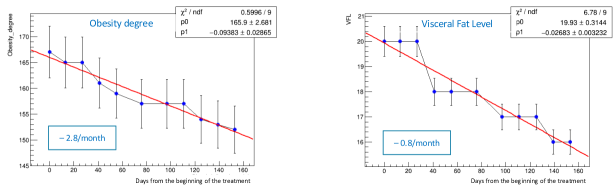
Figure 8: Trend line of the obesity degree, on the left, and VFL, on the right, as a function of the time from the beginning of the treatment. Both trends are linear with a 10% reduction of the obesity degree and a 20% reduction of the VFL in 5 months of treatment for the patient ID1556.

The study of the trend lines for the body circumferences is illustrated in Figure 9. The circumferences of waist, chest, hips, thigh, neck and arm are plotted as a function of the time from the beginning of the treatment. All circumferences drop linearly with time. Waist and arm circumferences decreased of 12% in 5 months, chest, hips and thigh of about 4-5%, neck of 7.5%.

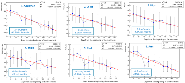
Figure 9: Trendlines of the body circumferences (Waist, Chest, Hips, Thigh, Neck, Arm) for the patient ID1556. All numbers on the vertical axis are expressed in cm.

Moreover, the study of the trend line for the difference between the weight and the target weight is shown in Figure 10. This patient lost almost 2 kg (constantly) per month of treatment reaching a 30% reduction of his weight in 5 months.

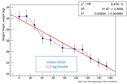
Figure 10: Trendline of the difference between the weight and the target weight (Weight-Target_weight for the patient ID1556.

6.2 Prediction of BIA parameters over time

In order to generalize the time behaviour observed for several BIA variables for each patient from the repeated fit procedure, we inferred a general behaviour associated to each cluster by observing the distributions of the parameters of the trend line (a and b) calculated for every patient within each cluster. These values were used to fill two histograms per cluster, one for the initial value of the considered variable a and the other for the monthly variation of that parameter b*30 days. From these, the mean and the standard deviation of these distributions can be calculated, so that a prediction of the time behaviour can be done this time at cluster-level.

As an example, the results related to cluster 5 are reported. Cluster 5 is the one corresponding to male patients that have a BMI slightly above average. In Figure 11 the distributions for the initial BMI and the BMI variation per month among all patients belonging to cluster 5 are shown. The second histogram contains the following information: if its mean value is negative, it means that, in average, these patients are decreasing their BMI value over the course of the diet, therefore losing weight; on the contrary, if its mean is positive, it means that they are increasing their BMI value, therefore gaining weight. In our case, the mean is about -0.5 BMI/month, which is an encouraging result since the cluster has an average initial value of 28.72 (Table 6).

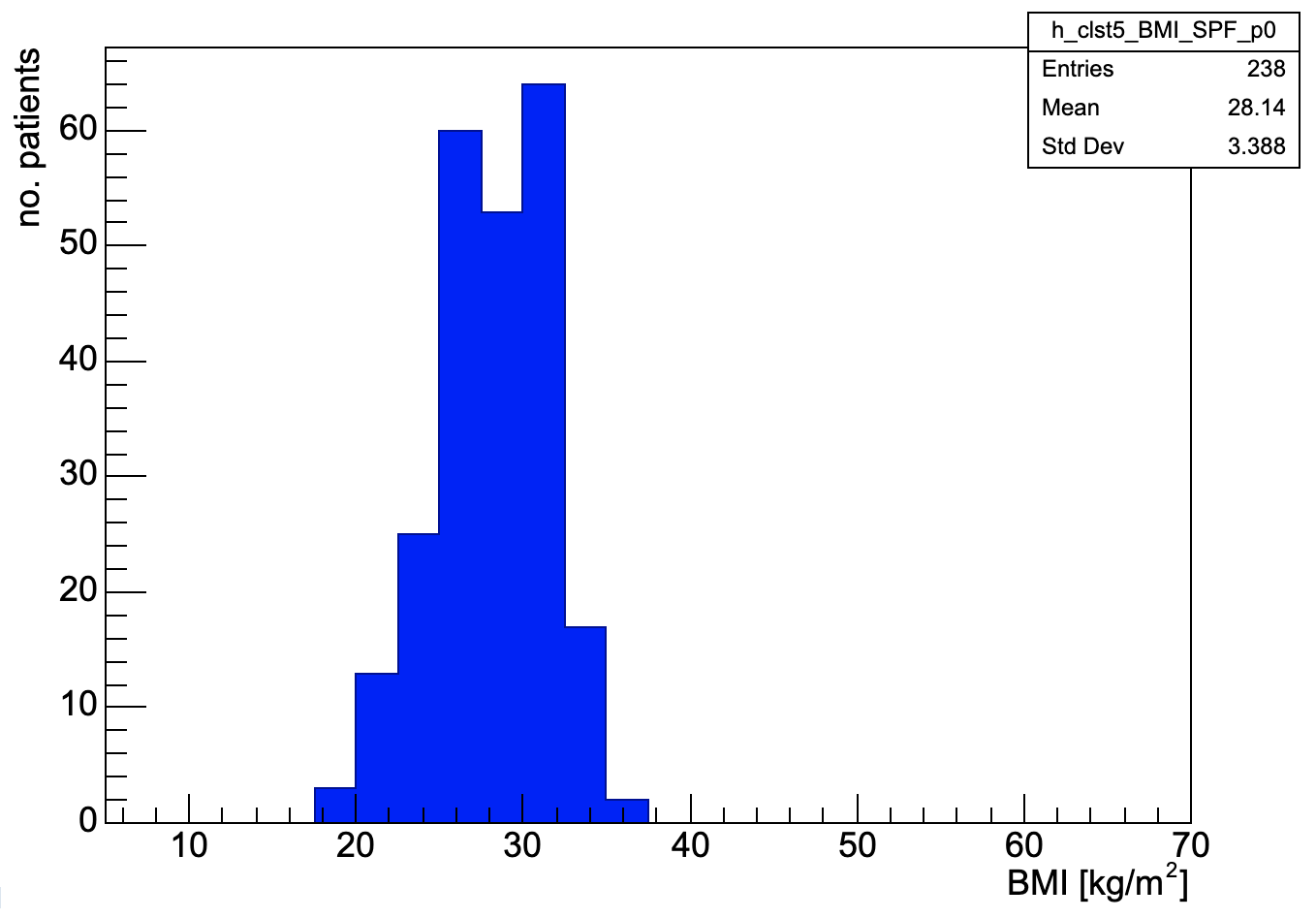
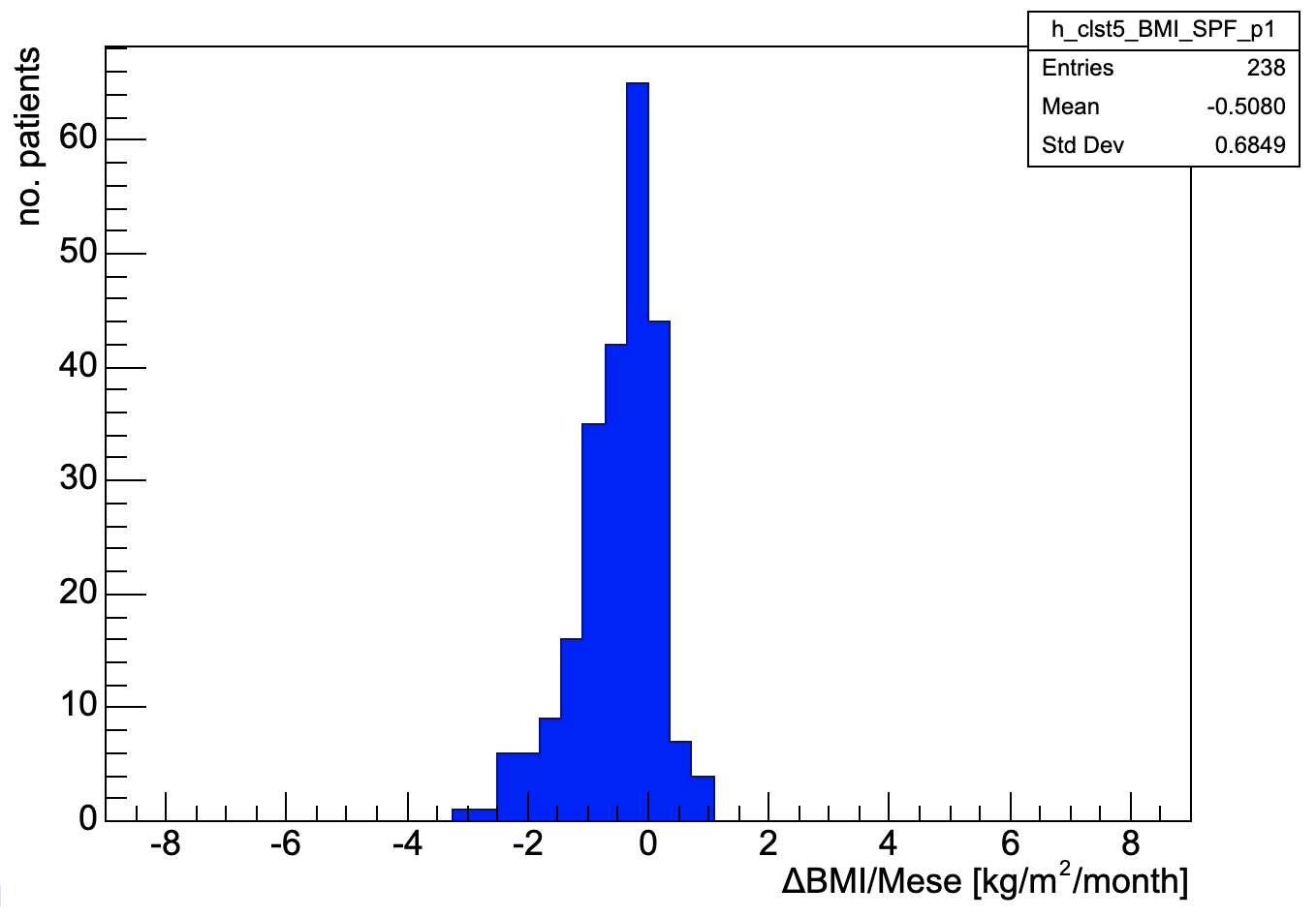
Figure 11: Distributions for patients in cluster 5 of the initial BMI values (on the left) and BMI variation per month (on the right) as obtained from the fit procedure.

An esteem of the number of months that would require for a patient in this cluster to reach a BMI value labelled as "Normal" can be obtained from the following equation:

$$\mathrm{N_{Months}}=\frac{(\mathrm{BMI_{ref}}-\mathrm{BMI_{0}})}{\Delta\mathrm{BMI/Month}}$$ (9)

where $\mathrm{BMI_{0}}$ is the mean initial BMI for the cluster, $\mathrm{BMI_{ref}}$ is the target BMI and $\Delta\mathrm{BMI/Month}$ is the mean BMI variation per month. For this particular case, the target BMI value of 24.9 would be reached, in average, with about 7 months of diet.

Finally, to have a quantitative comparison between initial and final values of the BIA variables for each cluster, we considered their percentage variation over the course of the diet. Again, taking as an example the BMI, this is defined as

$$\mathrm{percentage~{}variation~{}BMI}=\frac{\mathrm{final~{}BMI}-\mathrm{initial~{}BMI}}{\mathrm{initial~{}BMI}}*100$$ (10)

Filling a histogram with these values for each patient in cluster 5 (Figure 12) allowed us to determine how many of them had a benefit from the diet, based on the number of negatives (if the objective is to decrease the considered variable) or positives (if the objective is to increase the considered variable) over the number of patients in the cluster.

We can so see that about 77% of subjects improved their health condition by decreasing their BMI thanks to the proposed dietary treatment.

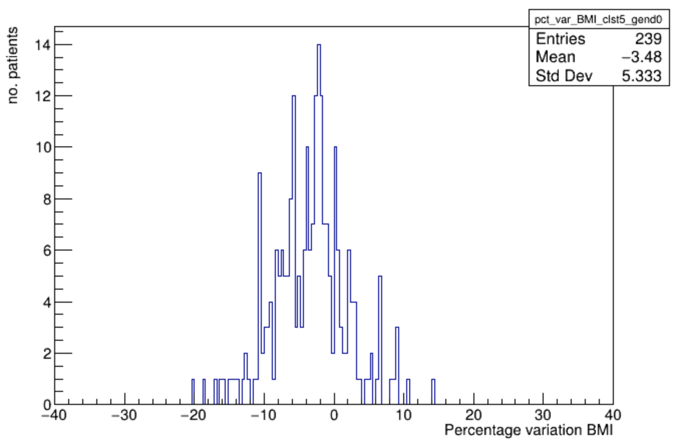
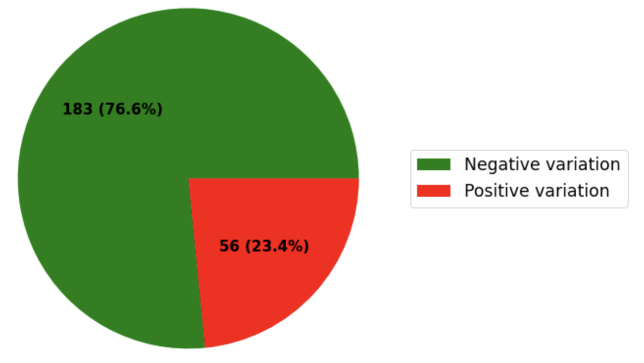
Figure 12: Distribution of the percentage variation of the BMI variable for cluster 5 patients and graph showing the fractions of negative and positive variations. More than 75% of these subjects showed an improvement in their BMI toward the "Normal" reference values.

7 Results of the Data Analysis

The analysis described in Section 6.1 and Section 6.2 is conducted for every patient and cluster. Trend lines are fitted to the selected variables for each patient within each cluster, and the mean values of these parameters are used to describe the trend for each cluster.

An overall quantitative comparison between initial and final values for each cluster is presented in Table 8, detailing the changes in BMI, WHR, and TBW. Across clusters 1 to 9, a significant reduction in BMI is observed, while cluster 10, characterized as underweight, shows a discrete increase. Similarly, WHR decreases for all clusters except those classified as underweight, where it remains stable, and very severely obese clusters, where it increases.

A similar comparison is also produced for the circumference of chest, trunk and hip, as reported in Table 9. Also in this case a consistent reduction is observed for all the cluster from 1 to 9 and a moderate increase for the cluster 10.

cluster	BMI [kg/m2]					WHR					TBW
	initial	final	$\Delta$[%]	$\Delta^{i}_{target}$[%]	$\Delta^{f}_{target}$[%]	initial	final	$\Delta$[%]	$\Delta^{i}_{target}$[%]	$\Delta^{f}_{target}$[%]	initial	final	$\Delta$[%]	$\Delta^{i}_{target}$[%]	$\Delta^{f}_{target}$[%]
1 - M, Very severely obese	55.80	48.25	-13.5	-55.4	-48.4	1.09	1.12	3.5	-17.1	-19.8	36.83	40.83	10.9	68.3	51.8
8 - M, Severely obese	41.45	38.84	-6.3	-39.9	-35.9	1.12	1.10	-1.5	-19.4	-18.2	42.50	44.71	5.2	45.9	38.7
5 - M, Overweight	28.72	27.60	-3.9	-13.3	-9.8	0.94	0.93	-1.9	-4.6	-2.8	52.29	53.81	2.9	18.6	15.2
9 - M, Moderately obese	34.56	32.74	-5.3	-28.0	-23.9	1.05	1.02	-2.8	-14.6	-12.0	46.38	48.45	4.5	33.7	28.0
7 - F, Normal weight, 35 yo	26.04	25.29	-2.9	-4.4	-1.5	0.90	0.89	-1.3	-11.3	-10.2	48.06	49.41	2.8	20.7	13.3
3 - F, Overweight, 55 yo	30.66	29.20	-4.8	-18.8	-14.7	0.97	0.95	-2.1	-17.8	-16.0	41.64	43.60	4.7	39.3	28.5
6 - F, Overweight, 27 yo	33.62	32.32	-3.9	-25.9	-23.0	0.99	0.97	-1.3	-18.8	-17.7	40.03	41.46	3.6	44.9	35.1
2 - F, Moderately obese, 44 yo	38.83	36.63	-5.7	-35.9	-32.0	1.04	1.02	-1.9	-22.9	-21.3	37.51	39.15	4.4	54.6	43.0
4 - Mix, Very severely obese	48.07	44.84	-6.7	-48.2	-44.5	1.04	1.07	2.1	-18.6	-20.2	35.42	36.63	3.4	69.4	63.8
10 - Mix, Underweight	18.82	19.09	1.5	0	0	0.79	0.79	0.1	0	0	58.24	58.21	-0.0	0	0

Table 8: Initial and final values and percent difference for each cluster for the BMI, WHR, and TBW variables.

Cluster	Chest circumference [cm]			Trunk circumference [cm]			Hip circumference [cm]
	initial	final	$\Delta$[%]	initial	final	$\Delta$[%]	initial	final	$\Delta$[%]
1 - M, Very severely obese	130.30	128.47	-1.4	153.53	147.38	-4.0	141.35	132.10	-6.5
8 - M, Severely obese	123.75	120.73	-2.4	137.94	132.41	-4.0	123.68	120.39	-2.7
5 - M, Overweight	104.99	103.33	-1.6	99.17	95.63	-3.6	104.86	103.08	-1.7
9 - M, Moderately obese	115.22	112.82	-2.1	120.62	114.68	-4.9	114.55	111.91	-2.3
7 - F, Normal weight, 35 yo	93.92	92.79	-1.2	88.40	86.20	-2.5	97.86	96.68	-1.2
3 - F, Overweight, 55 yo	100.04	97.84	-2.2	100.17	96.07	-41	102.94	100.80	-2.1
6 - F, Overweight, 27 yo	105.87	103.97	-1.8	107.73	104.47	-3.0	109.35	107.43	-1.8
2 - F, Moderately obese, 44 yo	113.87	110.48	-3.0	119.84	114.71	-4.3	115.71	112.74	-2.6
4 - Mix, Very severely obese	126.27	122.36	-3.1	134.27	132.13	-1.6	128.84	124.26	-3.6
10 - Mix, Underweight	78.22	78.94	0.9	66.56	66.92	0.6	84.54	84.90	0.4

Table 9: Initial and final values and percent difference for each cluster for the chest, trunk, and hip circumferences.

cluster	BMI [kg/m2]						WHR
	initial	$\Delta$/M	6 months	12 months	18 months	months for target	initial	$\Delta$/M	6 months	12 months	18 months	months for target
1 - M, Very severely obese	54.16	-1.4808	45.28	36.39	27.51	20	1.13	0.0024	1.14	1.16	1.17	-
8 - M, Severely obese	40.96	-1.5404	31.72	22.48	13.24	11	1.11	-0.0107	1.05	0.98	0.92	20
5 - M, Overweight	28.14	-0.5080	25.09	22.05	19.00	7	0.93	-0.0063	0.90	0.86	0.82	6
9 - M, Moderately obese	34.05	-0.6825	29.96	25.86	21.77	14	1.05	-0.0097	0.99	0.94	0.88	16
7 - F, Normal weight, 35 yo	25.77	-0.3186	23.86	21.95	20.04	3	0.90	-0.0041	0.88	0.85	0.83	25
3 - F, Overweight, 55 yo	30.35	-0.4639	27.57	24.78	22.00	12	0.97	-0.0003	0.97	0.97	0.96	518
6 - F, Overweight, 27 yo	33.19	-0.5163	30.09	26.99	23.89	17	0.98	-0.0026	0.97	0.95	0.94	72
2 - F, Moderately obese, 44 yo	38.46	-0.7203	34.14	29.81	25.49	19	1.03	-0.0071	0.99	0.95	0.91	33
4 - Mix, Very severely obese	47.23	-0.8186	42.32	37.41	32.50	28	1.04	0.0039	1.07	1.09	1.11	-
10 - Mix, Underweight	18.85	0.0474	19.14	19.42	19.71	0	0.79	0.0105	0.85	0.91	0.97	0

Table 10: Mean initial value, mean variation per month, predicted values at 6, 12 and 18 months and number of months to reach the target value for each cluster for BMI and WHR variables.

8 Conclusion

This paper reports a statistical analysis of the performance of a low insulin index, alkaline and functional diet developed by ANTUR. The dataset was divided in clusters with similar characteristics evaluated with a Self-organizing map, a machine learning method. The sample of patients was checked on a regular basis with a BioImpedenziometric analysis using 40 features describing the global health status of the patient. A study of the behaviour of the BIA parameters evolution over time with respect to the first visit was performed. More than the 75% of the patient that followed the ANTUR diet showed an improvement of the health status. The overall prediction for each cluster at fixed time periods, i.e. after 6, 12 and 18 months from the beginning of the diet, and the assumed number of months to reach the objective is reported in Table 10, detailing the BMI and WHR parameters. Assuming a constant linear trend, most of these results show that values within the reference ranges can be obtained in a reasonable time, depending of course by the severity of the starting health condition of the patients.

The method proposed permits to have an estimation of time needed to a patient to arrive to the target weight and, more globally, to a healthier state. This could be a very useful tool alongside traditional ones to define a dedicated and more efficient protocol for each patient. Moreover, having a timeline can help to motivate the patient to continue in following the protocol.

References

- [1] World Health Organization (WHO). Obesity and overweight. https://www.who.int/news-room/fact-sheets/detail/obesity-and-overweight, 2024.
- [2] Zeinab Faghfoori, Siavash Fazelian, Mahdi Shadnoush, and Reza Goodarzi. Nutritional management in women with polycystic ovary syndrome: A review study. Diabetes & Metabolic Syndrome: Clinical Research & Reviews, 11:S429–S432, 2017. SI: Online Supplement - 1.
- [3] S H Holt, J C Miller, and P Petocz. An insulin index of foods: the insulin demand generated by 1000-kj portions of common foods. Am J Clin Nutr, 66(5):1264–1276, November 1997.
- [4] Katharina Nimptsch, Jennie C Brand-Miller, Mary Franz, Laura Sampson, Walter C Willett, and Edward Giovannucci. Dietary insulin index and insulin load in relation to biomarkers of glycemic control, plasma lipids, and inflammation markers. The American Journal of Clinical Nutrition, 94(1):182–190, 2011.
- [5] M Modan, H Halkin, S Almog, A Lusky, A Eshkol, M Shefi, A Shitrit, and Z Fuchs. Hyperinsulinemia. a link between hypertension obesity and glucose intolerance. The Journal of Clinical Investigation, 75(3):809–817, 3 1985.
- [6] Benjamin C Fu, Fred K Tabung, Claire H Pernar, Weike Wang, Amparo G Gonzalez-Feliciano, Ilkania M Chowdhury-Paulino, Steven K Clinton, Edmund Folefac, Mingyang Song, Adam S Kibel, Edward L Giovannucci, and Lorelei A Mucci. Insulinemic and inflammatory dietary patterns and risk of prostate cancer. Eur. Urol., 79(3):405–412, March 2021.
- [7] Fu BC et al. Insulin resistance and prediabetes. national institute of diabetes and digestive and kidney diseases. https://www.niddk.nih.gov/healthinformation/diabetes/overview/what-is-diabetes/prediabetes-insulin-resistance, 2018.
- [8] Bianca N Quade, Mark D Parker, and Rossana Occhipinti. The therapeutic importance of acid-base balance. Biochem. Pharmacol., 183(114278):114278, January 2021.
- [9] Renata Alves Carnauba, Ana Beatriz Baptistella, Valéria Paschoal, and Gilberti Helena Hübscher. Diet-induced low-grade metabolic acidosis and clinical outcomes: A review. Nutrients, 9(6), May 2017.
- [10] et al. Wynn, E. Postgraduate symposium positive influence of nutritional alkalinity on bone health: Conference on ‘over- and under-nutrition: Challenges and approaches. Proceedings of the Nutrition Society, vol. 69, no. 1, 2010, pp. 166–173., doi:10.1017/S002966510999173X, 2010.
- [11] Smitha R Pillai, Mehdi Damaghi, Yoshinori Marunaka, Enrico Pierluigi Spugnini, Stefano Fais, and Robert J Gillies. Causes, consequences, and therapy of tumors acidosis. Cancer Metastasis Rev., 38(1-2):205–222, June 2019.
- [12] James L. Lewis III. Metabolic acidosis. https://www.msdmanuals.com/professional/endocrine-and-metabolic-disorders/acid-base-regulation-and-disorders/metabolic-acidosis, 2023.
- [13] Sara Farnetti. Tutto quello che sai sul cibo è falso. Conoscere gli alimenti e imparare a mixarli per un corpo sano e su misura. BUR Biblioteca Univ. Rizzoli, 2012.
- [14] Ahmad Alkhatib, Catherine Tsang, Ali Tiss, Theeshan Bahorun, Hossein Arefanian, Roula Barake, Abdelkrim Khadir, and Jaakko Tuomilehto. Functional foods and lifestyle approaches for diabetes prevention and management. Nutrients, 9(12), December 2017.
- [15] Serafini Mauro and Ilaria Peluso. Functional foods for health: The interrelated antioxidant and anti-inflammatory role of fruits, vegetables, herbs, spices and cocoa in humans. Current pharmaceutical design vol. 22,44 (2016): 6701-6715., 2016.
- [16] M Viuda-Martos, Y Ruiz-Navajas, J Fernández-López, and J A Pérez-Alvarez. Spices as functional foods. Crit. Rev. Food Sci. Nutr., 51(1):13–28, January 2011.
- [17] Ursula G Kyle, Ingvar Bosaeus, Antonio D De Lorenzo, Paul Deurenberg, Marinos Elia, José Manuel Gómez, Berit Lilienthal Heitmann, Luisa Kent-Smith, Jean-Claude Melchior, Matthias Pirlich, Hermann Scharfetter, Annemie M W J Schols, Claude Pichard, and Composition of the ESPEN Working Group. Bioelectrical impedance analysis–part i: review of principles and methods. Clin. Nutr., 23(5):1226–1243, October 2004.
- [18] W C Chumlea and S S Guo. Bioelectrical impedance and body composition: present status and future directions. Nutr. Rev., 52(4):123–131, April 1994.
- [19] Oliver Selberg and Daniela Selberg. Norms and correlates of bioimpedance phase angle in healthy human subjects, hospitalized patients, and patients with liver cirrhosis. Eur. J. Appl. Physiol., 86(6):509–516, April 2002.
- [20] C Faisy, A Rabbat, B Kouchakji, and J P Laaban. Bioelectrical impedance analysis in estimating nutritional status and outcome of patients with chronic obstructive pulmonary disease and acute respiratory failure. Intensive Care Med., 26(5):518–525, May 2000.
- [21] A Schwenk, A Beisenherz, K Römer, G Kremer, B Salzberger, and M Elia. Phase angle from bioelectrical impedance analysis remains an independent predictive marker in HIV-infected patients in the era of highly active antiretroviral treatment. Am. J. Clin. Nutr., 72(2):496–501, August 2000.
- [22] M Ott, H Fischer, H Polat, E B Helm, M Frenz, W F Caspary, and B Lembcke. Bioelectrical impedance analysis as a predictor of survival in patients with human immunodeficiency virus infection. J. Acquir. Immune Defic. Syndr. Hum. Retrovirol., 9(1):20–25, May 1995.
- [23] Digant Gupta, Carolyn A Lammersfeld, Jessica L Burrows, Sadie L Dahlk, Pankaj G Vashi, James F Grutsch, Sara Hoffman, and Christopher G Lis. Bioelectrical impedance phase angle in clinical practice: implications for prognosis in advanced colorectal cancer. Am. J. Clin. Nutr., 80(6):1634–1638, December 2004.
- [24] S Toso, A Piccoli, M Gusella, D Menon, A Bononi, G Crepaldi, and E Ferrazzi. Altered tissue electric properties in lung cancer patients as detected by bioelectric impedance vector analysis. Nutrition, 16(2):120–124, February 2000.
- [25] Q Maggiore, S Nigrelli, C Ciccarelli, C Grimaldi, G A Rossi, and C Michelassi. Nutritional and prognostic correlates of bioimpedance indexes in hemodialysis patients. Kidney Int., 50(6):2103–2108, December 1996.
- [26] L B Pupim, P Kent, and T A Ikizler. Bioelectrical impedance analysis in dialysis patients. Miner. Electrolyte Metab., 25(4-6):400–406, July 1999.
- [27] A Schwenk, L C Ward, M Elia, and G M Scott. Bioelectrical impedance analysis predicts outcome in patients with suspected bacteremia. Infection, 26(5):277–282, September 1998.
- [28] JA Máttar et al. Total body bioelectrical impedance measurement as a progressive outcome prediction and therapeutic index in the comparison between septic and non-septic patients. A multicenter Brazilian study. R Metab Nutr, 2(4):159–65, 1995.
- [29] Anja Bosy-Westphal, Sandra Danielzik, Ralf-Peter Dörhöfer, Wiebke Later, Sonja Wiese, and Manfred J Müller. Phase angle from bioelectrical impedance analysis: population reference values by age, sex, and body mass index. JPEN J. Parenter. Enteral Nutr., 30(4):309–316, July 2006.
- [30] Raffaella Cancello, Amelia Brunani, Ettore Brenna, Davide Soranna, Simona Bertoli, Antonella Zambon, Henry C Lukaski, and Paolo Capodaglio. Phase angle (PhA) in overweight and obesity: evidence of applicability from diagnosis to weight changes in obesity treatment. Rev. Endocr. Metab. Disord., 24(3):451–464, June 2023.
- [31] Bruna Ramos da Silva, Camila E Orsso, Maria Cristina Gonzalez, Juliana Maria Faccioli Sicchieri, Mirele Savegnago Mialich, Alceu A Jordao, and Carla M Prado. Phase angle and cellular health: inflammation and oxidative damage. Rev. Endocr. Metab. Disord., 24(3):543–562, June 2023.
- [32] Francesco Campa, Lucas Antonio Colognesi, Tatiana Moro, Antonio Paoli, Andrea Casolo, Leandro Santos, Rafael Ribeiro Correia, Ítalo Ribeiro Lemes, Vinícius Flávio Milanez, Diego Destro Christofaro, Edilson Serpeloni Cyrino, and Luís Alberto Gobbo. Effect of resistance training on bioelectrical phase angle in older adults: a systematic review with meta-analysis of randomized controlled trials. Rev. Endocr. Metab. Disord., 24(3):439–449, June 2023.
- [33] H C Lukaski. Biological indexes considered in the derivation of the bioelectrical impedance analysis. Am. J. Clin. Nutr., 64(3 Suppl):397S–404S, September 1996.
- [34] Jan Nyboer. Electrorheometric properties of tissues and fluids. Annals of the New York Academy of Sciences, 170(2):410–420, 1970.
- [35] C F Kay and H P Schwan. Specific resistance of body tissues. Circ. Res., 4(6):664–670, November 1956.
- [36] S M Guo, A F Roche, W C Chumlea, D S Miles, and R L Pohlman. Body composition predictions from bioelectric impedance. Hum Biol, 59(2):221–233, April 1987.
- [37] M A Thomasset. Bioelectric properties of tissue. impedance measurement in clinical medicine. significance of curves obtained. Lyon Med., 94:107–118, July 1962.
- [38] Antonino D Lorenzo and Angela Andreoli. Segmental bioelectrical impedance analysis. Curr. Opin. Clin. Nutr. Metab. Care, 6(5):551–555, September 2003.
- [39] E L Thomas, G Frost, T Harrington, and J D Bell. Validation of ‘inbody’ bioelectrical impedance by whole body mri. Technical report, The Robert Steiner MR Unit and 2Nutrition and Dietetic Research Group, Imperial College of Medicine, Hammersmith Hospital, London, 2001.
- [40] Teuvo Kohonen. Self-organized formation of topologically correct feature maps. Biological Cybernetics, 43(1):59–69, Jan 1982.
- [41] Juha Vesanto. Som-based data visualization methods. Intelligent Data Analysis, 3(2):111–126, 1999.
- [42] P. Smyth Fayyad, G. Piatetsky-Shapiro. From Data Mining to Knowledge Discovery: An Overview. Advances in Knowledge Discovery and Data Mining, AAAI Press/The MIT Press, 1996.