Exploring Intrinsic Bond Orbitals in Solids

Abstract

We present a study of the construction and spatial properties of localized Wannier orbitals in large supercells of insulating solids. The well-known Pipek-Mezey (PM) functional in combination with intrinsic atomic orbitals (IAOs) as projectors is employed, resulting in so-called intrinsic bond orbitals (IBOs). Independent of the bonding type and band gap, a correlation between orbital spreads and geometric properties is observed. As a result, comparable sparsity patterns of the Hartree-Fock exchange matrix are found across all considered bulk 3D materials, exhibiting covalent bonds, ionc bonds, and a mixture of both bonding types. Recognizing the considerable computational effort required to construct localized Wannier orbitals for large periodic simulation cells, we address the performance and scaling of different solvers for the localization problem. This includes the Broyden–Fletcher–Goldfarb–Shanno (BFGS), limited-memory BFGS (L-BFGS), Conjugate-Gradient (CG), and the Steepest Ascent (SA) method. Each algorithm performs a Riemannian optimization under unitary matrix constraint, efficiently reaching the optimum in the “curved parameter space” on geodesics. Also the Direct Inversion in the Iterative Subspace (DIIS) technique is employed. We observe that the construction of Wannier orbitals for supercells of metal oxides presents a significant challenge, requiring approximately one order of magnitude more iteration steps than other systems studied.

I Introduction

Localized orbitals are a useful tool in quantum chemistry and materials physics. They serve a variety of purposes, for example, the analysis of chemical bonds in tune with chemical intuition [1, 2], the investigation of electron transfer processes [3], the calculation of electron-phonon interactions [4], or the development of efficient many-electron correlation algorithms with reduced computational cost [5, 6, 7, 8, 9, 10, 11].

Known as localized Wannier orbitals in solid-state physics and localized molecular orbitals in quantum chemistry, they are usually derived from delocalized one-electron mean-field orbitals through rotations, achieved by a unitary matrix, resulting in spatial confinement. Various definitions have been proposed for determining this unitary matrix [12, 1, 13, 14], with several implementations available for periodic systems [15, 16, 17, 9, 18, 19, 20].

Here, we consider localized orbitals as a tool to introduce sparsity in Coulomb integrals, with the long-term goal of addressing the scaling problem in many-electron correlation methods. Our focus is on large simulation cells, which are essential for realistic models, for example, surface phenomena and defects. Consequently, we examine the scalability of constructing localized Wannier orbitals for large periodic cells of materials containing several hundred atoms. To this end we study the performance of various solvers. In addition to this technical investigation, we report an intriguing result that we found during our research: for all considered semiconductors the sparsity in the Fock exchange matrix is almost unaffected by the band gap of the material.

The paper is divided into two main parts, which follow after a brief theoretical summary of the definition of IBOs for solids and a desciription of the employed software packages and computational settings in Sec. II. The first main part is in Sec. III where we discuss the theory, implementation, and performance of the numerical construction of IBOs using different numerical solvers. The second main part is in Sec. IV where we report spatial properties of IBOs, an analysis of the sparsity of the Fock exchange matrix, and trends across the considered materials.

II Computational Methods & Intrinsic Bond Orbitals

All calculations are based on Hartree-Fock (HF) orbitals obtained from the plane-wave based Vienna Ab initio Simulation Package (VASP) [21, 22, 23]. Supercells are considered using a $\bm{\Gamma}$-only sampling of the Brillouin zone (BZ).

In this work, localized Wannier orbitals $|\mathcal{W}_{i}\rangle$ are obtained by a unitary transformation of the Bloch-like spin-orbitals $|\chi_{j}\rangle$,

$$|\mathcal{W}_{j}\rangle=\sum_{i}^{N_{\text{occ}}}\,u_{ij}\,|\chi_{i}\rangle\;,$$ (1)

where $u_{ij}$ is a unitary matrix. Since we focus on large supercells, no sum over the sampling points of the BZ appears in the definition of the Wannier orbitals. The matrix $u_{ij}$ is optimized to maximize (minimize) a localization functional $\mathcal{L}$, which defines the localized Wannier orbitals. Various localization functionals exist in the literature, such as Foster-Boys (FB) [12], Edmiston-Ruedenberg (ER) [1], von-Niessen (VN) [13], and Pipek-Mezey (PM) [14]. Our Riemannian optimization algorithm described in Sec. III.1.1 is suited for any cost functional, allowing us to compare the case of PM, FB, and VN. Since we employ $\bm{\Gamma}$-point-only sampling, the unitary matrices here are in fact real and orthogonal matrices.

Intrinsic bond orbitals were introduced by Knizia  [2] and are the result of maximizing the PM functional,

$$\mathcal{L}^{\text{PM}}[\{u_{ij}\}]=\sum_{i}^{N_{\text{occ}}}\sum_{A}^{N_{\text{atoms}}}|\,\langle\mathcal{W}_{i}|\bm{P}_{A}|\mathcal{W}_{i}\rangle\,|^{2}\;,$$ (2)

where $\bm{P}_{A}=\sum_{\mu\in A}|\mu\rangle\langle\mu|$ are projectors onto atom-centered functions $|\mu\rangle$, also known as IAOs. The IAOs are constructed from atomic functions $|f_{\mu}\rangle$ via the projection:

$$|\mu^{\text{IAO}}\rangle=(\mathds{1}+\mathcal{O}-\widetilde{\mathcal{O}})|f_{\mu}\rangle\;,$$ (3)

where $\mathcal{O}$ is the projector onto the occupied space and $\widetilde{\mathcal{O}}$ projects onto the space spanned by occupied orbitals from a minimal atomic basis. These projectors are defined as:

$$\mathcal{O}=\sum_{i}^{N_{\text{occ}}}|\chi_{i}\rangle\langle\chi_{i}|\;,\quad\widetilde{\mathcal{O}}=\sum_{i}^{N_{\text{occ}}}|\widetilde{\chi}_{i}\rangle\langle\widetilde{\chi}_{i}|\;,$$ (4)

with the orbitals $|\widetilde{\chi}_{i}\rangle$ given by

$$|\widetilde{\chi}_{i}\rangle=\text{orth}\left[\,\sum_{\mu\nu}|f_{\mu}\rangle\,S^{-1}_{\mu\nu}\,\langle f_{\nu}|\chi_{i}\rangle\,\right]\;,$$ (5)

where $S_{\mu\nu}=\langle f_{\mu}|f_{\nu}\rangle$ is the overlap matrix of the atomic functions. The ”orth” denotes orthogonalization.

The orbitals $|\widetilde{\chi}_{i}\rangle$ approximate the occupied orbitals in the minimal atomic basis $|f_{\mu}\rangle$, while the exact occupied mean-field orbitals $|\chi_{i}\rangle$ are obtained from a preceding mean-field calculation in the plane-wave basis, which is considered a complete basis. The term $\mathcal{O}-\widetilde{\mathcal{O}}$ in Eq. (3) augments the atomic functions to form the IAOs, ensuring completeness of the occupied space. As long as no occupied orbital is orthogonal to the atomic functions, i.e., $\sum_{\nu}\langle f_{\nu}|\chi_{i}\rangle\neq 0$, $\forall i$, the IAOs form an exact atom-centered basis for the occupied space.

III Construction of Intrinsic Bond Orbitals

Similar to the IBOs, most localization methods start by defining an orbital-dependent cost function, $\mathcal{L}$, which is then optimized using an iterative algorithm. Hence, finding efficient algorithms is vital. As described previously in Sec. II, we employ the PM method to obtain IBOs. Optimization is performed using a Riemannian geometry approach. Underlying works on these topics were conducted for example by Luenberger and Gabay [24, 25].

III.1 Riemannian optimization under unitary constraint

Riemannian optimization leverages the theory of optimization and concepts of differential geometry, more specifically Riemannian manifolds. We follow the works of Abrudan et al. [26, 27] and Huang et al. [28, 29].

III.1.1 Optimization

Iteratively, a minimum (or maximum) of some function $\mathcal{L}(\bm{U})$ shall be approached, where $\bm{U}$ represents an abstract vector in the parameter space. The optimization algorithms we compare are Conjugate-Gradient (CG), limited-memory BFGS (L-BFGS)and Steepest Ascent (SA)solvers, in this paper we focus particularly on the first two, as SA has proven to be clearly inferior in our calculations and in Refs. [18, 20]. Being line search methods, first a suitable direction is chosen and subsequently an optimal step size along the chosen path is to be found. Valuable explanations regarding these topics can be found in reference [30]. On its own, these algorithms are unrestricted within the respective parameter space, and follow the general update formula

$$\bm{U}_{k+1}=\bm{U}_{k}+\alpha_{k}\bm{H}_{k}$$ (6)

with the iterates $\bm{U}_{k+1}$ and $\bm{U}_{k}$ being estimates of the desired extremum, the step size $\alpha$ and the search direction $\bm{H}$.

While for SA $\bm{H}$ just equals the gradient $\bm{\nabla}\mathcal{L}(\bm{U}_{k})$, CG is calculated according to the formula:

$$\bm{H}_{k}=\bm{\nabla}\mathcal{L}(\bm{U}_{k})+\beta\bm{H}_{k-1}$$ (7)

with $H_{0}=\bm{\nabla}\mathcal{L}(\bm{U}_{0})$ and $\beta$ is a mixing factor. In our work we chose the Polak-Ribière (PR) factor [31, 32].

The quasi-newton L-BFGS [33] is an approximation of the BFGS, which forms a quadratic model of the function locally and calculates the search direction as $\bm{H}=-\bm{B}\bm{\nabla}\mathcal{L}(\bm{U}_{k})$, with $\bm{B}$ as the models’ approximated inverse Hessian according to the BFGS formula

$$\bm{B}_{k+1}=(\bm{I}-\rho_{k}\bm{y}_{k}\bm{s}_{k}^{T})\bm{B}_{k}(\bm{I}-\rho_{k}\bm{y}_{k}\bm{s}_{k}^{T})+\rho_{k}\bm{s}_{k}\bm{s}_{k}^{T}$$ (8)

where $\bm{I}$ is the $N\times N$ identity matrix, $N$ being the number of parameters,

$$\rho_{k}=\frac{1}{\bm{y}_{k}^{T}\bm{s}_{k}},$$ (9)

and

$$\bm{s}_{k}=\bm{U}_{k+1}-\bm{U}_{k},\quad\bm{y}_{k}=\bm{\nabla}\mathcal{L}_{k+1}-\bm{\nabla}\mathcal{L}_{k}$$ (10)

For an inverse of the Hessian to exist, the so-called curvature condition $\bm{s}_{k}^{T}\bm{y}_{k}>0$ must hold. This can be ensured by deploying a step size algorithm that is based on the Wolfe conditions [30], for example. While BFGS stores the matrix $\bm{B}$ of size $N^{2}$ at every step, the limited memory version L-BFGS approximates equation (8) iteratively, therefore only storing vectors $\bm{y}$ and $\bm{s}$ of size $N$ from a memory of past steps (note that in our case, $\bm{y}$ and $\bm{s}$ are matrices of size $n\times n$, so the total number of parameters $N$ is $n^{2}$). This makes the method suitable for large scale problems with a high dimensional parameter space, while the regular BFGS is only applicable to small systems. With increasing memory size, L-BFGS approaches the inverse Hessian of BFGS and if every step is memorized they are mathematically equivalent at the $N^{\text{th}}$ iteration. Consequently, L-BFGS is usually the method of choice for large $N$. When setting the memory size to 1, L-BFGS is closely related to CG methods, which also memorize the gradient at the preceding point to update the search direction [30].

Finally, when a search direction is calculated by one of the above methods, a suitable step size has to be found. After all, the search direction only selects the path and doesn’t determine an exact point along that path already. Step size algorithms are in general independent of the way search directions are selected, although some are more suitable than others. Abrudan et al. suggest interpolating along the search path and calculating the maximum (minimum) of the resulting polynomial [27] to obtain a reasonable estimate. Another example for a method suitable for L-BFGS is based on the Hager-Zhang scheme [34].

III.1.2 Riemannian Geometry and Lie groups

To guarantee the unitary property of our parameter matrix $\bm{U}$, Riemannian manifolds, smooth manifolds equipped with a metric, are introduced. In general, a smooth manifold $M$ is a topological space that fulfills special requirements regarding distance, neighborhood and differentiability. Locally it is closely connected to Euclidean spaces via homomorphic mapping. For a more detailed treatment of the concepts in this chapter, especially in the context of optimization, consider the references [35, 29, 27].

To each point $\bm{U}$ of a manifold, a tangent space $T_{\bm{U}}M$ is attached, i.e., the set of all possible tangent vectors at that point. An important aspect of these tangent spaces is the existence of mapping procedures between tangent spaces and the manifold, a textbook example is the exponential map (see Eq.(13)), which enables movement along curves on the manifold. Hereby, tangent vectors define the curves’ directions. A Riemannian metric is defined on each tangent space as inner product $g(\bm{X},\bm{Y})=\langle\bm{X},\bm{Y}\rangle$, where $\bm{X},\bm{Y}$ are tangent vectors. Here, we chose the Frobenius norm.

A key property of unitary $n\times n$ matrices is that they form a Lie group $U(n)$, with matrix multiplication as a group action. The tangent space of the point at unity is highlighted as the Lie algebra $\mathfrak{u}$ of the group.

One of the important concepts is the map of right (and left) translation, meaning the multiplication of a point $\bm{V}\in U(n)$ by another point on the right (or left):

$$\begin{matrix}R_{U}:&U(n)&\rightarrow&U(n)\\ &\bm{V}&\mapsto&\bm{V}\bm{U}\end{matrix}$$ (11)

and equivalently for left translation.

It can be shown that a tangent vector $X_{\bm{V}}\in T_{\bm{V}}U(n)$ can be translated in the same way to another tangent space $T_{\bm{V}\bm{U}}U(n)$:

$$\begin{matrix}R_{U*}:&T_{\bm{V}}U(n)&\rightarrow&T_{\bm{V}\bm{U}}U(n)\\ &\bm{X}_{\bm{V}}&\mapsto&\bm{X}_{\bm{V}}\bm{U}&\equiv&\bm{X}_{\bm{V}\bm{U}}\end{matrix}$$ (12)

Importantly, these translations are isometries with respect to the riemannian metric in the case of $U(n)$, so distances are preserved, allowing curves to be ”moved” easily from point to point. This enables us to perform calculations solely in the Lie algebra. From every tangent vector in the Lie algebra, $X_{I}\in T_{\bm{I}}U(n)\equiv\mathfrak{u}$, it follows from equation (12) that it can be moved to any tangent space $T_{\bm{U}}U(n)$ by simply multiplying by $\bm{U}$ from the right: $\bm{X}_{\bm{U}}=\bm{X}_{\bm{I}}\bm{U}$ and vice versa every tangent vector can be easily translated to the Lie algebra: $\bm{X}_{\bm{I}}=\bm{X}_{\bm{U}}\bm{U}\textsuperscript{\textdagger}$.

The exponential mapping $\exp:\mathfrak{u}\rightarrow U(n)$ connects the Lie algebra to the group, in our case this is simply the matrix exponential of any skew-hermitian matrix $\bm{X}$,

$$\text{exp}(\alpha\bm{X})=\bm{\gamma}(\alpha)$$ (13)

where the curve $\bm{\gamma}:\mathbb{R}\rightarrow U(n)$ is a parameterized geodesic and therefore the shortest path between two points of the group. This can be understood as taking a direction $\bm{X}$ and moving along a geodesic with the velocity $\alpha$.

III.1.3 Combining the Concepts

Combining the two concepts, optimization algorithms naturally designed as unrestricted in the Euclidean parameter space can be generalized to Riemannian manifolds with inherently enforced restrictions, in our case on unitary matrices. As derived by Abrudan et al. [26], the gradient of a function $\mathcal{L}(\bm{U})$ at some point $\bm{U}$ is given by

$$\bm{\nabla}\mathcal{L}(\bm{U})=\bm{\Gamma}-\bm{U}\bm{\Gamma}\textsuperscript{\textdagger}\bm{U}$$ (14)

where $\bm{\Gamma}$ is the Euclidean derivative matrix $d\mathcal{L}/du_{ij}$. Subsequently, this gradient is translated to the Lie algebra via right translation:

$$\bm{G}(\bm{U})\equiv\bm{\nabla}\mathcal{L}(\bm{U})\bm{U}\textsuperscript{\textdagger}=\bm{\Gamma}\bm{U}\textsuperscript{\textdagger}-\bm{U}\bm{\Gamma}\textsuperscript{\textdagger}$$ (15)

The algorithms SA, CG and BFGS are now following section III.1.1, utilizing the translated gradient $\bm{G}(\bm{U})$ to obtain the search direction $\bm{H}$. This vector is mapped to the group using the exponential map in equation (13), the emanating curve $\text{exp}(\alpha\bm{H})$ is transported to $\bm{U}_{k}$, obtaining $\bm{U}_{k+1}$:

$$\bm{U}_{k+1}=\text{exp}(\alpha\bm{H})\bm{U}_{k}$$ (16)

where the scaling factor $\alpha$ serves as step size.

III.2 Implementation

The VASP implementation for the L-BFGS solver is shown in Algorithm 1, following the work of Huang et al. and Nocedal et al. [28, 30]. The two-loop recursion was developed by Nocedal et al. [30] and efficiently computes the L-BFGS search direction. For the step size calculations, we utilize the method developed by Abrudan et al. [27]. To validate our implementation and confirm our results, we repeated all calculations using the manopt.jl package by Bergmann et al. [36, 37], where we selected a step size algorithm based on the Hager-Zhang scheme [34]. The Eucledian derivative for the IBOs reads

$$\Gamma^{\text{PM}}_{ij}=\frac{\partial\mathcal{L}^{\text{PM}}}{\partial u^{*}_{ij}}$$ (17)

$$=2\sum_{A}^{N_{\text{atoms}}}\sum_{k}^{N_{\text{occ}}}\langle\chi_{i}|\bm{P}_{A}|\chi_{k}\rangle\,u_{kj}\bigg{|}\sum_{lm}^{N_{\text{occ}}}\langle\chi_{l}|\bm{P}_{A}|\chi_{m}\rangle\,u^{*}_{lj}\,u_{mj}\bigg{|}\;.$$

Algorithm 1 L-BFGS algorithm implementation

choose memory size m, break condition $\epsilon$

choose starting point $U_{0}$

calculate the initial gradient $G(U_{0})$ from equation (15)

$s_{i},y_{i},\rho_{i}\leftarrow 0$

$\lambda\leftarrow 1$

$k\leftarrow 0$

repeat

     $k\leftarrow k+1$

     procedure two-loop recursion

         $q\leftarrow G(U_{k})$

         for $i=m,m-1,...,1$ do

              $a_{i}\leftarrow\rho_{i}g(s_{i},q)$

              $q\leftarrow q-a_{i}y_{i}$

         end for

         $r\leftarrow\lambda q$

         for $i=1,...,m$ do

              $b\leftarrow\rho_{i}g(y_{i},r)$

              $r\leftarrow r+s_{i}(a_{i}-b)$

         end for

         $H_{k}\leftarrow-r$

     end procedure

     perform step size algorithm to obtain $\alpha_{k}$

     $U_{k+1}=\text{exp}(\alpha_{k}H_{k})U_{k}$

     calculate $G(U_{k+1})$

     for $i=1,...,m-1$ do

         $s_{i}\leftarrow s_{i+1},\quad$ $y_{i}\leftarrow y_{i+1},\quad$ $\rho_{i}\leftarrow\rho_{i+1}$,

     end for

     $s_{m}\leftarrow\alpha_{k}H_{k}$

     $y_{m}\leftarrow G(U_{k+1})-G(U_{k})$

     $\rho_{m}\leftarrow 1/g(s_{m},y_{m})$

     $\lambda\leftarrow g(s_{m},y_{m})/g(y_{m},y_{m})$

until $||G(U_{k})||<\epsilon$

III.3 Results

To check our code for robustness and efficiency, we performed computations for numerous systems, including molecules, molecular crystals, bulk solids, as well as large supercells with broken translational symmetry. If not stated otherwise, calculations were initialized with random unitary matrices and a break condition for the gradient norm of $10^{-5}$ was chosen as criterion for convergence. We measure the performance of an algorithm by the number of iterations required to reach convergence.

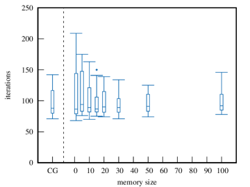
Figure 1: Number of required iterations against the number of memorized L-BFGS steps compared to CG for a graphene supercell (162 atoms) with flowerdefects.

Surprisingly, specifically for periodic systems, large L-BFGS memory sizes do not necessarily lead to improved performance, which is shown in Fig.1 for a graphene flowerdefect (supercell with 324 occupied orbitals). But the statistical variance of the required number of iterations decreases with higher memory while the rise in computational cost is negligible. If not stated otherwise, a fixed memory size of 20 is used for our L-BFGS calculations. Note that CG and L-BFGS perform similar for this example, an observation that is consistent across all tested periodic systems.

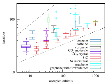
Figure 2: L-BFGS iterations against occupied orbitals, several systems and supercell sizes are compared. The dashed lines are proportional to $\sqrt{n}$ and $\sqrt[4]{n}$ respectively, giving an idea of scaling.

Fig. 2 shows the number of necessary iterations against the system size for a selected set of systems using the L-BFGS solver. Interestingly, for supercells with broken symmetry L-BFGS shows a similar performance as for the pristine case, as the results for the flowerdefect graphene and Si with interstitial defects indicate. The increase in iterations with higher system size is roughly proportional to the fourth root of the number of occupied orbitals $n$, as demonstrated by the dashed lines. Consequently, the increase is proportional to the square root of the number of optimization parameters $n^{2}$, i.e., the number of matrix entries.

material / molecule	#occ	L-BFGS	CG	SA
benzene	12	49	83	7093
caffeine	37	97	132	3217
coronene	54	65	85	671
CO2 molecule	8	31	38	171
CO2 crystal	32	51	53	269
	256	73	81	316
SiC	16	26	26	54
	32	33	33	68
	72	41	41	87
	128	47	45	102
	180	51	50	110
	256	56	53	120
	432	63	58	134
defect Si	1040	84	74	154
graphene	64	50	51	124
	256	89	78	197
	576	76	67	155
flowerdefect graphene	324	90	88	265

Table 1: Comparison of the median number of iterations for L-BFGS, CG and SA convergence for several systems.

In Tab. 1, the median number of required iterations are listed for L-BFGS, CG and SA algorithms. While SA is clearly inferior to the others for all test systems, apparently L-BFGS has an advantage over CG only for molecules.

material	#occ	largest maximum		second largest maximum
		iterations	cost per #occ	iterations	cost per #occ
graphene	64	49 (92%)	1.1357	112 (8%)	1.1278
	256	87 (90%)	1.1346	126 (7%)	1.1293
	576	76 (100%)	1.1430	0 (0%)
flowerdefect	324	83 (62%)	1.1350	119 (38%)	1.1341

Table 2: For several graphene supercells, the algorithms not always converge to the same value of the cost function. The percentage of runs (out of 60 each) converging to the respective maximum is given in brackets. Notably, when converging to a lower value, the number of iterations is considerably larger. These outliers are also visible in Fig. 2 for the graphene cells.

Notably, some graphene cells exhibit outliers with a substantially higher number of iterations, approaching other local extrema. This behavior, visible in Fig.2, is further quantified in Tab. 2 for the L-BFGS algorithm. For example, flowerdefect graphene (324 occupied orbitals) calculations converge to a slightly worse maximum in 38 of runs. The same observations was confirmed with the manopt.jl package considering CG and L-BFGS, and using a different line search method.

material	oxide	#occ	IBO	FB	VN
SiC	non-oxide	256	53	140	39
CO2	molecular oxide crystal	256	81	546	294
SiO2	non-metal oxide	288	155	496	154
TiO2	metal oxide	288	678	1628	605
MgO	metal oxide	288	1737	1464	365

Table 3: Comparison of the the average number of necessary iterations for metal oxides and a set of other materials employing the intrinsic bond orbital (IBO), Foster-Boys (FB), and von-Niessen (VN)localization functionals. Supercells containing a comparable number of occupied orbitals were considered. The average was calculated from 4 runs initialized with random unitary matrices.

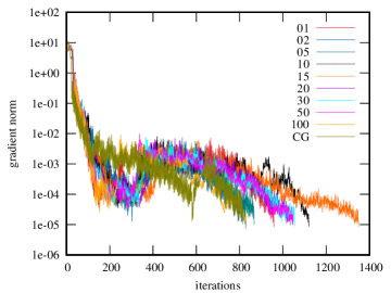
Figure 3: Convergence of L-BFGS with several memory size settings and CG, for a TiO2 supercell (72 atoms, 288 occupied orbitals), the unity matrix serves as starting point (i.e. starting from bloch orbitals).

An interesting exception are metal oxides, listed in Tab. 3. Here, all considered localization functionals IBO, FB and VN show a similar trend. Metal oxides require about one order of magnitude more iterations for a fixed convergence threshold. As example, the slow and erratic decrease of the gradient norm can be seen in Fig. 3 for a TiO2 supercell (72 atoms, 288 occupied orbitals).

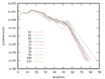
Figure 4: Convergence of L-BFGS with several memory size settings and CG, for a graphene supercell (162 atoms) with flowerdefects, the unity matrix serves as starting point (i.e. starting from bloch orbitals).

In contrast, a typical convergence pattern of non-oxides is shown in Fig. 4 using the aforementioned graphene flowerdefect supercell as an example. From a certain iteration step onwards (in this case somewhere between 50 and 60 iterations), convergence is consistently exponential.

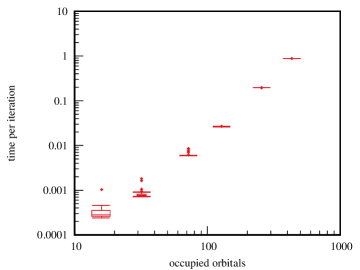
Figure 5: L-BFGS runtime per iteration in seconds against occupied orbitals, $n$, of SiC supercells, showing a $n^{3}$ scaling.

The relation between L-BFGS runtime per iteration and system size is depicted in Fig. 5 for SiC. Except for very small cells, where the overall insignificant impact of several inexpensive routines is visible, the runtime scales proportionally to $n^{3}$, where $n$ is the number of occupied orbitals. This behavior is expected, as $n$ determines the size of most of the involved matrices and, consequently, the cost of matrix operations. CG and SA are only marginally faster, on average by $3.5\%$ and $4.1\%$ respectively, disregarding the smallest two cells. It can be stated, that the additional complexity of L-BFGS is insignificant in relation to the cost of other routines like gradient calculation or line search algorithm.

A Comment on the DIIS Technique

We implemented a Direct Inversion in the Iterative Subspace (DIIS)technique to investigate its potential for accelerating convergence to the optimum. Our implementation was modeled after the documentation by C. D. Sherrill [38]. Essentially, the DIIS technique is a mixer that seeks to find optimal linear combinations of previous iteration steps. This technique is well-established for accelerating iterative solvers in finding the HF ground state. When finding an optimal unitary matrix, this matrix must be parametrized to construct linear combinations of previous solutions, resulting in a new unitary matrix. While several parametrizations exist [39], we used the exponential parametrization.

We applied the DIIS technique on top of our discussed solvers, which generate the trial vectors and residuals for DIIS. The number of trial vectors and residuals was tested in the range of 5 to 20. Additionally, a threshold for the gradient norm was set and tested within the range of $10^{-1}$ to $10^{-4}$ to ensure the DIIS solver did not start before the gradient norm fell below this threshold.

Although our DIIS implementation outperformed the SA solver, it did not demonstrate any advantage over the CG or BFGS solvers with our settings. While we cannot conclusively state that no effective DIIS implementation exists for accelerating convergence, we did not pursue this approach further due to our negative results.

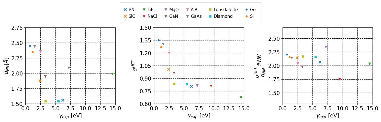
Figure 6: Plot of the nearest neighbor distance $d_{\text{NN}}$ (left), the IBO orbital spread $\sigma_{\text{HF}}$ (centre), and relation between orbitals spread and $d_{\text{NN}}/\#\text{NN}$ (right) plotted against the experimental band gap of all considered materials.

III.4 Discussion

In this first part of the paper, we considered the performance of various solvers, avoiding any bias such as initial guesses. In contrast to previous studies of Clement et al. [18], we cannot confirm a significant advantage of L-BFGS over CG for any of the examined problems. Both are substantially more efficient than the SA, each in their Riemannian version respectively. The similar performance of CG and L-BFGS, and the latter’s weak dependence of memory size, indicate that Hessian approximations, at least the BFGS approximation, are not particularly beneficial for many problems. However, L-BFGS iterations are only marginally slower than CG and SA in runtime measurements, dispelling a potential disadvantage and indicating the runtime dominance of other routines like gradient calculation or step size search. Runtime per iteration scales cubically with the number of occupied orbitals.

For several graphene supercells, a certain percentage of runs approach slightly different maxima, a behavior that is persistent for all tested solvers.

We find that some metal oxides converge significantly slower than other test systems and speculate that this issue is due to the ionic character of the material. The localized orbitals exhibit similar shape as atomic orbitals and superpositions of these atomic-like orbitals leave the cost function almost untouched. This adds to the potential problem of local extrema and saddle points, which are very typical for high dimensional cost functions.

These challenges highlight the necessity for improvements such as good initial guesses or even better solvers, also the development of new localization functionals should be considered.

Note, that comparison with other works which model solids via small primitive cells and $\bm{k}$-point sampling [40, 18, 20] should be taken with care, as we employ a supercell formulation using a single $\bm{k}$-point, the $\bm{\Gamma}$-point, for sampling the Brillouin Zone (BZ) due to our focus on material models with large cells and broken translational symmetry.

IV Properties of Intrinsic Bond Orbitals

In the second main part of the paper, we investigate spatial properties of IBOs for a variety of insulating solids, as listed in Tab. 4. These IBOs were constructed from Hartree-Fock (HF) orbitals, and their spatial character were analyzed in relation to the material’s crystal structure and band gap. A focus was the average orbital spread of the IBOs and its relationship with geometric properties, specifically the nearest neighbor distance ($d_{\text{NN}}$) and the number of nearest neighbors ($\#\text{NN}$). Our findings reveal that the orbital spread per nearest neighbor distance, multiplied by the number of nearest neighbors, remains relatively stable across the materials considered. This can be captured by the empirical relation $\sigma_{\text{HF}}\approx 2.1\alpha$, where $\alpha=\frac{d_{\text{NN}}}{\#\text{NN}}$. This trend was consistent across various crystal structures, independent of the band gap, providing a useful estimate for predicting the spatial extent of localized orbitals (see Fig. 6).

	structure	bond	$a[\AA]$	$d_{\text{NN}}[\AA]$	$\#\text{NN}$	$\sigma_{\text{HF}}[\AA]$	$\gamma_{\text{exp}}[eV]$
C (Diamond)	A4	covalent	3.57	1.54	4	0.832	5.48
Si	A4	covalent	5.431	2.35	4	1.268	1.17
Ge	A4	covalent	5.652	2.45	4	1.351	0.74
NaCl	B1	ionic	5.569	2.78	6	0.813	9.50
MgO	B1	ionic	4.189	2.09	6	0.817	7.22
LiF	B1	ionic	3.972	1.99	6	0.676	14.5
SiC	B3	mixed	4.346	1.88	4	1.009	2.42
BN	B3	mixed	3.592	1.56	4	0.806	6.22
AlP	B3	ionic	5.451	2.36	4	1.204	2.51
GaAs	B3	ionic	5.64	2.44	4	1.307	1.52
GaN	B3	ionic	4.509	1.95	4	0.966	3.30
C (Lonsdaleite)	B4	covalent	4.347	1.54	4	0.835	3.35

Table 4: List of considered materials. The structure column refers to the Strukturbericht designation. Mixed bonds have ionic and covalent character. The lattice constant $a$, the nearest neighbor distance $d_{\text{NN}}$, the number of nearest neighbors $\#\text{NN}$, the IBO orbital spread $\sigma_{\text{HF}}$, and the experimental band gap $\gamma_{\text{exp}}$ are also provided.

We also analyzed the decay of the Fock exchange matrix entries,

$$J_{\mu\nu}=-\frac{1}{2}\int\text{d}^{3}r_{1}\int\text{d}^{3}r_{2}\frac{\varphi^{*}_{\mu}(\bm{r}_{1})\varphi_{\nu}(\bm{r}_{1})\;\varphi^{*}_{\nu}(\bm{r}_{2})\varphi_{\mu}(\bm{r}_{2})}{|\bm{r}_{1}-\bm{r}_{2}|}\;,$$ (18)

in the basis of Wannier orbitals $\varphi_{\mu}$. Two methods were employed to estimate the error per atom when truncating these matrix entries. This error is defined as

$$\varepsilon=\left|\sum_{\mu\nu}J_{\mu\nu}-\sum_{\mu\nu}^{\text{trunc.}}J_{\mu\nu}\right|/N_{A}\;,$$ (19)

where $N_{A}$ is the number of atoms. Method 1 involves zeroing out matrix elements below a certain threshold (Fig.  7), while Method 2 uses a cutoff radius based on the distance between Wannier orbitals (Fig. 8). It is striking that no significant difference can be observed between germanium and diamond, for example. Note that germanium is a small-gap materials with an experimental band gap of $0.74\,\text{eV}$ and a high relative permittivity compared to diamond with a band gap of $3.35\,\text{eV}$ and is significantly less polarizable.

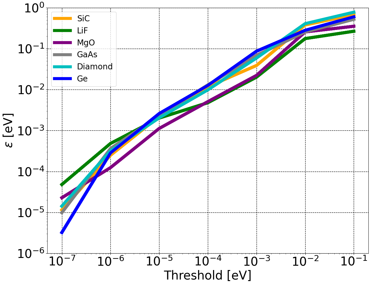
Figure 7: Error per atom $\varepsilon$ for different thresholds of the Exchange matrix entries using the truncation method 1 (see text for explanation).

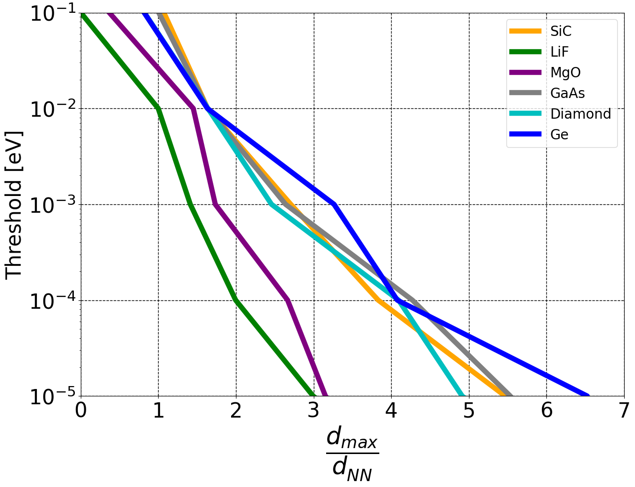
Figure 8: Error per atom with respect to the largest distance between the Wannier orbitals $d_{\text{max}}$ per nearest neighbour distance, using the truncation method 2 (see text for explanation)

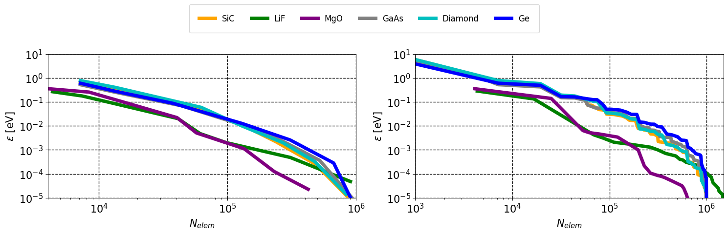
Figure 9: Fock exchange energy error per atom $\varepsilon$ with respect to the number of non-zero elements $N_{\text{elem}}$ of the Fock matrix using the truncation method 1 (left) and 2 (right), as explained in the text.

Our findings on the truncation of the Fock exchange matrix further support the potential for computational savings due to its sparsity. This holds for both large-gap and small-gap materials, suggesting that the band gap has a relatively minor effect on the decay of matrix elements for practical purposes. Figure 9 shows the number of remaining non-zero Fock exchange matrix elements in dependence of $\varepsilon$ for both methods.

In summary, the analysis of IBO properties across various materials reveals a correlation between orbital spread and geometric factors. This relationship provides a straightforward way to estimate the spatial extent of localized orbitals, which is crucial for the development of reduced-cost methods. Additionally, the truncation of the Fock exchange matrix demonstrates significant potential for reducing computational costs in large-scale simulations, with manageable errors across a wide range of materials.

V Conclusion

In this work we studied the numerical construction and spatial properties of IBOs based on HF orbitals for a set of insulating solids. We reported a relation between the orbital spread measured in units of the nearest neighbor distance and the number of nearest neighbors. Independent of the band gap, this relation is relatively stable for all considered 3D semiconductors. It suggests that local methods based on the sparsity of Coulomb integrals can also be applied to materials with small band gaps without losing the sparsity. We verified this hypothesis for the particular case of the sparsity of the Fock exchange matrix in the basis of IBOs. Whether this can be extended to metallic solids or scenarios involving localized unoccupied orbitals, essential for many-electron correlation methods, remains an open question. This warrants further investigation in future work.

Additionally, we benchmarked various solvers to optimize the unitary matrix that transforms delocalized Bloch orbitals into localized Wannier orbitals, specifically in the form of IBOs. Our focus was on large simulation cells, which are crucial for realistic models, such as those involving surface phenomena and defects. Contrary to some previous studies, we did not observe a clear performance advantage of the L-BFGS solver, instead finding that both the CG and L-BFGS solvers exhibited similar performance. When using stochastic (unbiased) starting points, we found that constructing localized orbitals in supercells of metal oxides pose a significant challenge, requiring an order of magnitude more iteration steps than for the other materials considered. This emphasizes the importance of well-chosen starting points and the potential value of non-iterative methods for constructing localized Wannier orbitals in solids.

References

- Edmiston and Ruedenberg [1963] C. Edmiston and K. Ruedenberg, Localized atomic and molecular orbitals, Reviews of Modern Physics 35, 457 (1963).
- Knizia [2013] G. Knizia, Intrinsic atomic orbitals: An unbiased bridge between quantum theory and chemical concepts, Journal of Chemical Theory and Computation 9, 4834 (2013).
- Knizia and Klein [2015] G. Knizia and J. E. Klein, Electron flow in reaction mechanisms—revealed from first principles, Angewandte Chemie International Edition 54, 5518 (2015).
- Engel et al. [2020] M. Engel, M. Marsman, C. Franchini, and G. Kresse, Electron-phonon interactions using the projector augmented-wave method and wannier functions, Physical Review B 101, 184302 (2020).
- Voloshina et al. [2011] E. Voloshina, D. Usvyat, M. Schütz, Y. Dedkov, and B. Paulus, On the physisorption of water on graphene : a ccsd(t) study, Physical Chemistry Chemical Physics 13, 12041 (2011).
- Usvyat et al. [2018] D. Usvyat, L. Maschio, and M. Schütz, Periodic and fragment models based on the local correlation approach, WIREs Computational Molecular Science 8, 1 (2018).
- Kubas et al. [2016] A. Kubas, D. Berger, H. Oberhofer, D. Maganas, K. Reuter, and F. Neese, Surface adsorption energetics studied with “gold standard” wave-function-based ab initio methods: Small-molecule binding to tio 2 (110), The Journal of Physical Chemistry Letters 7, 4207 (2016).
- Schäfer et al. [2021a] T. Schäfer, F. Libisch, G. Kresse, and A. Grüneis, Local embedding of coupled cluster theory into the random phase approximation using plane waves, The Journal of Chemical Physics 154, 011101 (2021a).
- Schäfer et al. [2021b] T. Schäfer, A. Gallo, A. Irmler, F. Hummel, and A. Grüneis, Surface science using coupled cluster theory via local wannier functions and in-rpa-embedding: The case of water on graphitic carbon nitride, The Journal of Chemical Physics 155, 244103 (2021b).
- Lau et al. [2021] B. T. G. Lau, G. Knizia, and T. C. Berkelbach, Regional embedding enables high-level quantum chemistry for surface science, The Journal of Physical Chemistry Letters 12, 1104 (2021).
- Ye and Berkelbach [2024] H.-Z. Ye and T. C. Berkelbach, Adsorption and vibrational spectroscopy of co on the surface of mgo from periodic local coupled-cluster theory, Faraday Discussions 10.1039/D4FD00041B (2024).
- Foster and Boys [1960] J. M. Foster and S. F. Boys, Canonical configurational interaction procedure, Reviews of Modern Physics 32, 300 (1960).
- von Niessen [1973] W. von Niessen, Density localization of atomic and molecular orbitals - iii. heteronuclear diatomic and polyatomic molecules, Theoretica Chimica Acta 29, 29 (1973).
- Pipek and Mezey [1989] J. Pipek and P. G. Mezey, A fast intrinsic localization procedure applicable for a b i n i t i o and semiempirical linear combination of atomic orbital wave functions, The Journal of Chemical Physics 90, 4916 (1989).
- Zicovich-Wilson et al. [2001] C. M. Zicovich-Wilson, R. Dovesi, and V. R. Saunders, A general method to obtain well localized wannier functions for composite energy bands in linear combination of atomic orbital periodic calculations, The Journal of Chemical Physics 115, 9708 (2001).
- Marzari et al. [2012] N. Marzari, A. A. Mostofi, J. R. Yates, I. Souza, and D. Vanderbilt, Maximally localized wannier functions: Theory and applications, Reviews of Modern Physics 84, 1419 (2012).
- Jónsson et al. [2017] E. O. Jónsson, S. Lehtola, M. Puska, and H. Jónsson, Theory and applications of generalized pipek–mezey wannier functions, Journal of Chemical Theory and Computation 13, 460 (2017).
- Clement et al. [2021] M. C. Clement, X. Wang, and E. F. Valeev, Robust pipek–mezey orbital localization in periodic solids, Journal of Chemical Theory and Computation 17, 7406 (2021).
- Ozaki [2024] T. Ozaki, Closest wannier functions to a given set of localized orbitals, Physical Review B 110, 125115 (2024).
- Zhu and Tew [2024] A. Zhu and D. P. Tew, Wannier function localization using bloch intrinsic atomic orbitals, The Journal of Physical Chemistry A 10.1021/ACS.JPCA.4C04555 (2024).
- Kresse and Hafner [1993] G. Kresse and J. Hafner, Ab initio molecular dynamics for liquid metals, Physical Review B 47, 558 (1993).
- Kresse and Furthmüller [1996a] G. Kresse and J. Furthmüller, Efficient iterative schemes for ab initio total-energy calculations using a plane-wave basis set, Physical Review B 54, 11169 (1996a).
- Kresse and Furthmüller [1996b] G. Kresse and J. Furthmüller, Efficiency of ab-initio total energy calculations for metals and semiconductors using a plane-wave basis set, Computational Materials Science 6, 15 (1996b).
- Luenberger [1972] D. G. Luenberger, The gradient projection method along geodesics, Management Science 18, 620 (1972).
- Gabay [1982] D. Gabay, Minimizing a differentiable function over a differential manifold, Journal of Optimization Theory and Applications 37, 177 (1982).
- Abrudan et al. [2008] T. E. Abrudan, J. Eriksson, and V. Koivunen, Steepest descent algorithms for optimization under unitary matrix constraint, IEEE Transactions on Signal Processing 56, 1134 (2008).
- Abrudan et al. [2009] T. Abrudan, J. Eriksson, and V. Koivunen, Conjugate gradient algorithm for optimization under unitary matrix constraint, Signal Processing 89, 1704 (2009).
- Huang et al. [2015] W. Huang, K. A. Gallivan, and P.-A. Absil, A broyden class of quasi-newton methods for riemannian optimization, SIAM Journal on Optimization 25, 1660 (2015).
- Huang [2013] W. Huang, Optimization algorithms on Riemannian manifolds with applications, Ph.D. thesis, The Florida State University (2013).
- Nocedal and Wright [1999] J. Nocedal and S. J. Wright, Numerical optimization (Springer, 1999).
- Polak and Ribiere [1969] E. Polak and G. Ribiere, Note sur la convergence de méthodes de directions conjuguées, Revue française d’informatique et de recherche opérationnelle. Série rouge 3, 35 (1969).
- Polak [1971] E. Polak, Computational methods in optimization: a unified approach, Vol. 77 (Academic press, 1971).
- Liu and Nocedal [1989] D. C. Liu and J. Nocedal, On the limited memory bfgs method for large scale optimization, Mathematical programming 45, 503 (1989).
- Hager and Zhang [2005] W. W. Hager and H. Zhang, A new conjugate gradient method with guaranteed descent and an efficient line search, SIAM Journal on Optimization 16, 170 (2005), https://doi.org/10.1137/030601880 .
- Qi [2011] C. Qi, Numerical optimization methods on Riemannian manifolds, Ph.D. thesis, The Florida State University (2011).
- Bergmann [2022] R. Bergmann, Manopt.jl: Optimization on manifolds in Julia, Journal of Open Source Software 7, 3866 (2022).
- Axen et al. [2023] S. D. Axen, M. Baran, R. Bergmann, and K. Rzecki, Manifolds.jl: An extensible julia framework for data analysis on manifolds, ACM Transactions on Mathematical Software 49, 10.1145/3618296 (2023).
- Sherrill [2004] C. D. Sherrill, Some comments on accelerating convergence of iterative sequences using direct inversion of iterative subspace (diis), Acessado em http://vergil. chemistry. gatech. edu/notes/diis. Setembro (2004).
- Shepard et al. [2015] R. Shepard, S. R. Brozell, and G. Gidofalvi, The representation and parametrization of orthogonal matrices, Journal of Physical Chemistry A 119, 7924 (2015).
- Lehtola and Jónsson [2013] S. Lehtola and H. Jónsson, Unitary optimization of localized molecular orbitals, Journal of chemical theory and computation 9, 5365 (2013).