Can the quantum switch be deterministically simulated?

Abstract

Higher-order transformations that act on a certain number of input quantum channels in an indefinite causal order—such as the quantum switch—cannot be described by standard quantum circuits that use the same number of calls of the input quantum channels. However, the question remains whether they can be simulated, i.e., whether their action on their input channels can be deterministically reproduced, for all arbitrary inputs, by a quantum circuit that uses a larger number of calls of the input channels. Here, we prove that when only one extra call of each input channel is available, the quantum switch cannot be simulated by any quantum circuit. We demonstrate that this result is robust by showing that, even when probabilistic and approximate simulations are considered, higher-order transformations that are close to the quantum switch can be at best simulated with a probability strictly less than one. This result stands in stark contrast with the known fact that, when the quantum switch acts exclusively on unitary channels, its action can be simulated.

I Introduction

Indefinite causal order is a property that emerged from the study of higher-order transformations in quantum theory [1, 2, 3, 4, 5]. While a quantum channel is a transformation that maps a quantum state into a quantum state, a transformation that maps a quantum channel into a quantum channel is a called a higher-order transformation. More generally, a higher-order transformation may take several arbitrary quantum channels as input and output a quantum channel. An example of such a transformation is a quantum circuit with “open slots” where arbitrary quantum channels can be inserted, giving rise to a higher-order transformation that acts on the input channels in a sequential, temporally-ordered manner, known as a quantum comb [1, 3]. Remarkably, there also exist well-defined higher-order transformations that act on their input quantum channels in an indefinite causal order [6, 7, 8]. Such transformations cannot be described by any quantum circuit that uses the same number of calls of the input quantum channels. Indefinite causal order has been shown to provide advantages in several quantum computation and information-theoretic tasks, such as quantum channel discrimination [9, 10, 11], quantum metrology [12, 13], computational complexity [14], query complexity [15], transformations of blackbox unitaries and isometries [16, 17, 18, 19], among others.

A prominent example of indefinite causal order that is responsible for several of these theoretically predicted advantages is the quantum switch [6], a higher-order transformation that coherently controls the causal order of two quantum channels $A$ and $B$. The information-processing advantages of the quantum switch have mostly been shown in comparison with higher-order transformations that act in a fixed order on a single call of quantum channels $A$ and $B$  [9, 8, 12, 10]. However, their true practical significance hinges on the extent to which these advantages would still hold when comparing the quantum switch with higher-order transformations that use a larger number of calls to the input quantum channels in a fixed order.

More concretely, this question can be phrased in terms of the simulability of the quantum switch, or more generally, of any higher-order transformation with indefinite causal order:

Can a higher-order transformation with indefinite causal order that acts on arbitrary quantum channels be simulated by standard quantum circuits that have access to more calls of the input quantum channels?

In the case where the quantum circuit performing the simulation has access to an infinite number of calls of the input channels, the answer is: yes. In this case, a process tomography protocol [3, 20, 21] can completely characterize the input channels and simply prepare the output channel expected from the higher-order transformation with indefinite causal order. However, such a simulation requires infinite resources. Another possible way that the quantum switch can be simulated is using probabilistic post-selection [6, 22]. However, such a simulation does not work deterministically. Additionally, in the particular case where the input channels are restricted to being unitary channels, it has been shown that a simulation of the quantum switch exists [6]. However, such a simulation is not universal.

We hence ask the question, which has remained largely unexplored so far: does any finite number of extra calls of the input channels suffice to deterministically and universally simulate the action of the quantum switch with a quantum circuit?

In this work, we prove that the quantum switch cannot be deterministically and universally simulated by a quantum circuit that has access to one extra call of each input quantum channel. We demonstrate the robustness of this result in two different ways. The first is by showing that even when probabilistic heralded simulations are considered, the maximum probability of a successful simulation is significantly below one. The second is by showing that even when approximate simulations are considered, the probability of simulating a higher-order operation which is $\epsilon$-close to the quantum switch is significantly below one for an $\epsilon$ significantly above zero. We furthermore thoroughly analyze the problem of simulating the quantum switch when it acts only on part of its input quantum channels or on quantum instruments. Finally, we show some new particular cases in which simulations of the quantum switch are possible. Our proof techniques are based on a method of basis design, semidefinite programming, and computer-assisted proofs.

From an experimental perspective, the question we answer in this work is also of key relevance. So far, the quantum switch has been the subject of several experiments (see, e.g., the review in Ref. [23]). A crucial point in the analysis of the experimental implementations of the quantum switch is whether the collected experimental data demonstrates indefinite causal order or if there exists a causal model that would be able to reproduce it. In particular, several implementations leave room for speculation that the experimental setup might be taking advantage of two available calls of each input channel, in contrast to the single call of each required by the quantum switch. A pressing question in this context is then whether the availability of an extra call of each quantum channel allows for a causal explanation of the experiment; in other words, whether the observed experimental data is compatible with a quantum circuit acting on two independent calls of each input quantum channel. Here, we show that this is not the case.

II Results

II.1 The simulation task

To simulate a higher-order transformation with indefinite causal order is to reproduce its action on any arbitrary set of input channels using another higher-order transformation that obeys some causal constraints and has access to more calls of the input channels. In this work, we focus in particular on simulations of the quantum switch.

The quantum switch $\mathcal{S}$ is defined as a higher-order transformation that takes two arbitrary quantum channels (i.e., completely positive, trace-preserving maps) $A$ and $B$ as input, where $A:\mathcal{L}(\mathcal{H}^{A_{I}})\to\mathcal{L}(\mathcal{H}^{A_{O}})$ and $B:\mathcal{L}(\mathcal{H}^{B_{I}})\to\mathcal{L}(\mathcal{H}^{B_{O}})$ are channels that act on qudit systems, and transforms them into a channel $\mathcal{S}(A,B):\mathcal{L}(\mathcal{H}^{c_{I}}\otimes\mathcal{H}^{t_{I}})\to\mathcal{L}(\mathcal{H}^{c_{O}}\otimes\mathcal{H}^{t_{O}})$ that acts on a qubit control system and a qudit target system. The output channel resulting from the action of the switch on its input channels is defined as [6]

$$\mathcal{S}(A,B)[\,\sigma_{c}\otimes\rho_{t}\,]\coloneqq\sum_{i,j}S_{ij}(\sigma_{c}\otimes\rho_{t})S_{ij}^{\dagger},$$ (1)

where $\sigma_{c}\in\mathcal{L}(\mathcal{H}^{c_{I}})$ is the the state of the input qubit control system, $\rho_{t}\in\mathcal{L}(\mathcal{H}^{t_{I}})$ is that of the qudit target system, and $S_{ij}$ is given by

$$S_{ij}\coloneqq\outerproduct{0}{0}\otimes B_{j}A_{i}+\outerproduct{1}{1}\otimes A_{i}B_{j},$$ (2)

where $\{A_{i}\}_{i}$ and $\{B_{j}\}_{j}$ are Kraus representations [24] of the channels $A$ and $B$, respectively; i.e., $A[\rho]=\sum_{i}A_{i}\,\rho\,A_{i}^{\dagger}$ and $B[\rho]=\sum_{i}B_{i}\,\rho\,B_{i}^{\dagger}$. This transformation is depicted in Fig. 1. The quantum switch has been interpreted as a higher-order transformation that displays a quantum control of causal orders. That is, the quantum switch acts on its input channels in a different order that is conditioned on the state of a quantum control system. Since the quantum control system may be initiated in a superposition state such as $\ket{+}\coloneqq\frac{1}{\sqrt{2}}(\ket{0}+\ket{1})$, the overall quantum switch transformation may be understood as a superposition of two different circuits, one with the control system in state $\ket{0}$ and the quantum channels being applied in the order $A$ before $B$, and another with the control system in state $\ket{1}$ and the quantum channels being applied in the order $B$ before $A$.

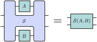
Figure 1: The quantum switch transformation. The quantum switch is a higher-order transformation that takes as input two quantum channels, $A$ and $B$, and transforms them into a different quantum channel $\mathcal{S}(A,B)$. The resulting channel $\mathcal{S}(A,B)$ acts on a qubit control system and a qudit target system.

A simulation of the quantum switch is a higher-order transformation $\mathcal{C}$ that obeys causal constraints and that acts on $k_{A}$ calls of the channel $A$ and $k_{B}$ calls of the channel $B$ in such a way that the channel $\mathcal{C}(A^{\otimes k_{A}},B^{\otimes k_{B}}):\mathcal{L}(\mathcal{H}^{c_{I}}\otimes\mathcal{H}^{t_{I}})\to\mathcal{L}(\mathcal{H}^{c_{O}}\otimes\mathcal{H}^{t_{O}})$ resulting from this transformation satisfies

$$\mathcal{C}(A^{\otimes k_{A}},B^{\otimes k_{B}})=\mathcal{S}(A,B)\ \ \ \forall\ A,B,$$ (3)

where $A,B$ are arbitrary quantum channels. Natural causal constraints that one might impose on the simulation is to require that $\mathcal{C}$ be described by a standard quantum circuit with open slots, i.e., a quantum comb [1, 3]. A more general strategy for the simulation—which could nevertheless be interpreted as “causal”—would be to impose that $\mathcal{C}$ is described by quantum circuits under classical control. This set of higher-order transformations, proposed in Ref. [25] and called quantum circuits with classical control of causal order (QC-CC), is larger than the set of standard quantum combs, allowing for classical mixing of different quantum circuits as well as for classical controlled dynamical causal orders. Hence, permitting this class gives more power to the simulation as compared to quantum combs, while still allowing for a causal interpretation of the simulation. In App. A we provide formal definitions of these causal constraints. We furthermore require the simulation to be universal: the same simulation $\mathcal{C}$ must work for all input pairs of quantum channels. Moreover, the simulation is required to be exact and deterministic, i.e., $\mathcal{C}(A^{\otimes k_{A}},B^{\otimes k_{B}})$ must be always exactly equal to $\mathcal{S}(A,B)$ for every pair of quantum channels $A$ and $B$. See Fig. 2 for a graphical representation of Eq. (3).

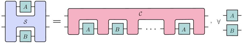
Figure 2: Simulating the quantum switch. A higher-order transformation $\mathcal{C}$, which can be a quantum comb or a QC-CC, that acts on several copies of the input quantum channels $A$ and $B$ is a simulation of the quantum switch $\mathcal{S}$ if it reproduces the action of the quantum switch for all arbitrary channels $A$ and $B$.

The question of simulability then boils down to whether there exists, for some finite number of calls $k_{A}$ and $k_{B}$, a simulation $\mathcal{C}$ that obeys causal constraints and that satisfies Eq. (3).

The task of simulating the quantum switch can be intuitively phrased as a game, which allows us to understand the universality aspect of the simulation in operational terms. Consider two players: one who can implement the quantum switch, while the other can only implement higher-order transformations with causal constraints. In this game, a referee provides the two players a pair of input channels $A$ and $B$ in the form of blackbox operations, which means they are unknown to the players, and challenges them to prepare the channel $\mathcal{S}(A,B)$. The player that can implement the switch can always win the game by deterministically preparing $\mathcal{S}(A,B)$ for every pair of unknown input channels, and can moreover do so using only a single copy of each channel. On the other hand, it is not clear whether the player that must obey causal constraints, called the simulator, can win the game. In other words, does their exist a finite number of calls that allows them to deterministically prepare $\mathcal{S}(A,B)$ for every pair of unknown input channels given by the referee?

II.2 A first (unsuccessful) attempt

In order to highlight the difficulty of the task of the simulator, let us analyze a potential strategy based on a naïve intuition of quantum control and understand why it fails. Suppose that the simulator is allowed an extra call of each input channel, i.e., $k_{A}=k_{B}=2$. A naïve strategy that the simulator might attempt is to implement the quantum circuit

$$\quantikz[columnsep=7mm]&\ctrl{2}\ctrl{2}\\ \targX{}\gate[style={fill=JessicaColour!30},labelstyle=black]{B}\gate[style={fill=JessicaColour!30},labelstyle=black]{A}\targX{}\\ \targX{}\gate[style={fill=JessicaColour!30},labelstyle=black]{A}\gate[style={fill=JessicaColour!30},labelstyle=black]{B}\targX{}$$ (4)

where $\quantikz[columnsep=1.5mm,rowsep=3.5mm]&\ctrl{2}\\ \targX{}\\ \targX{}$ is a control-SWAP gate. The above circuit prepares a channel $\mathcal{C}(A^{\otimes 2},B^{\otimes 2}):\mathcal{L}(\mathcal{H}^{c_{I}}\otimes\mathcal{H}^{\text{aux}_{I}}\otimes\mathcal{H}^{t_{I}})\to\mathcal{L}(\mathcal{H}^{c_{O}}\otimes\mathcal{H}^{\text{aux}_{O}}\otimes\mathcal{H}^{t_{O}})$. From top to bottom, the first line in the circuit in Eq. (4) corresponds to the control qubit system, the second line to an auxiliary qudit system, and the third line to the target qudit system.

By exploiting two calls of each input operation, the above circuit could also be interpreted as a higher-order transformation with quantum control of causal orders: For a control state prepared in a superposition $\ket{+}=\frac{1}{\sqrt{2}}(\ket{0}+\ket{1})$, the input channels are applied in a controlled superposition of the order $A$ before $B$ with the order $B$ before $A$. In fact, in several experiments concerning the quantum switch, there could be a margin to argue that a similar transformation as the one in Eq. (4) is being implemented by the experimental setup.

However, it is straightforward to see that the above circuit does not implement the same transformation as the quantum switch. The channel $\mathcal{C}(A^{\otimes 2},B^{\otimes 2})$ resulting from the circuit in Eq. (4) can be described by Kraus operators $\{C_{iji^{\prime}j^{\prime}}\}_{iji^{\prime}j^{\prime}}$, where

$$C_{iji^{\prime}j^{\prime}}\coloneqq\outerproduct{0}{0}\otimes A_{i^{\prime}}B_{j^{\prime}}\otimes B_{j}A_{i}+\outerproduct{1}{1}\otimes B_{j}A_{i}\otimes A_{i^{\prime}}B_{j^{\prime}}.$$ (5)

Consider the case where the channels $A$ and $B$ are restricted to having a single Kraus operator. This is the case where the input channels are unitary channels, which are a particular subset of quantum channels that map pure states into pure states. In this case, the resulting channel in Eq. (5) is also unitary. Now, fix the input states to be pure. When tracing out the output auxiliary system, the resulting transformation from the circuit in Eq. (4) is not equivalent to the quantum switch transformation $\mathcal{S}(A,B)$. This can be seen because, in general, the channel in Eq. (5) entangles the auxiliary system with the control and target systems. Hence, when the output auxiliary system is discarded, the resulting output control and target systems are not in a pure state, as they must be for the quantum switch.

Here, the highly non-trivial aspect of the problem of simulating the quantum switch becomes apparent—the quantum control of causal orders that is constructed by this quantum circuit using two calls of each input quantum channel is not equivalent to the quantum control of causal orders that is constructed by the quantum switch using a single call of each input quantum channel, and, therefore, it is not a valid simulation. Not only is this particular circuit not a simulation of the quantum switch, but as we prove in Sec. II.4, there does not exist any quantum circuit that can simulate the action of the switch with an extra call of each input operation.

II.3 Go-theorem: an explicit non-universal simulation

For a particular case of input channels, nevertheless, the quantum switch can be simulated. As first shown in the paper that originally defined the quantum switch [6], a simulation that requires only an extra use of one of the input quantum channels is possible, in the particular case where the input channels are unitary. The simulation presented in Ref. [6] is given by the quantum circuit

$$\quantikz[columnsep=6.5mm]&\ctrl{2}\ctrl{2}\ctrl[open]{2}\ctrl[open]{2}\\ \targX{}\targX{}\targX{}\targX{}\\ \targX{}\gate[style={fill=JessicaColour!30},labelstyle=black]{A}\targX{}\gate[style={fill=JessicaColour!30},labelstyle=black]{B}\targX{}\gate[style={fill=JessicaColour!30},labelstyle=black]{A}\targX{}$$ (6)

where $\quantikz[columnsep=1mm]&\ctrl[open]{0}$ $\coloneqq$ $\quantikz[columnsep=1mm]&\gate{X}\ctrl{0}\gate{X}$ and $\quantikz[columnsep=1mm]&\gate{X}$ is the NOT gate. Here again, the first circuit line corresponds to the control qubit system, the second to an auxiliary system, and the third to the target qudit system. This circuit can equivalently be represented by the Kraus operators $\{C_{iji^{\prime}}\}_{iji^{\prime}}$, where

$$C_{iji^{\prime}}\coloneqq\outerproduct{0}{0}\otimes A_{i^{\prime}}\otimes B_{j}A_{i}+\outerproduct{1}{1}\otimes A_{i}\otimes A_{i^{\prime}}B_{j}.$$ (7)

Although it is straightforward to see that the resulting transformation does not simulate the quantum switch for arbitrary quantum channels, it does so in the special case where the inputs are unitary channels. Notice that in this case—in contrast with the circuit in Eq. (4)—since $A_{i}=A_{i}^{\prime}$, the operation acting on the auxiliary space can be factored out, implying that the auxiliary system does not become entangled with the control or target systems.

Another crucial point to note is that the circuit in Eq. (6) acts on the input channels in the order “ABA”. If one were to change the order of the input channels to either “AAB” or “BAA”, this circuit no longer simulates the quantum switch, even if the input channels are unitary. In fact, for these different orders, we prove that there does not exist any quantum circuit that can simulate the action of the quantum switch, even when acting only on unitary channels. We present more details in App. D.

In this work, we show that an extension of the circuit in Eq. (6) allows one to perform a simulation of the quantum switch in a more general—albeit not fully general—scenario. This is the case where the quantum switch acts only on part of a quantum channel $A$ that is unitary and part of a quantum channel $B$ that is general.

In this simulation scenario, the quantum switch acts only on part of bipartite channels $A:\mathcal{L}(\mathcal{H}^{A_{I}}\otimes\mathcal{H}^{A^{\prime}_{I}})\to\mathcal{L}(\mathcal{H}^{A_{O}}\otimes\mathcal{H}^{A^{\prime}_{O}})$ and $B:\mathcal{L}(\mathcal{H}^{B_{I}}\otimes\mathcal{H}^{B^{\prime}_{I}})\to\mathcal{L}(\mathcal{H}^{B_{O}}\otimes\mathcal{H}^{B^{\prime}_{O}})$, both of which have two input and two output spaces. The output channel from the quantum switch transformation is then given by $\mathcal{S}\otimes\mathcal{I}(A,B):\mathcal{L}(\mathcal{H}^{A^{\prime}_{I}}\otimes\mathcal{H}^{c_{I}}\otimes\mathcal{H}^{t_{I}}\otimes\mathcal{H}^{B^{\prime}_{I}})\to\mathcal{L}(\mathcal{H}^{A^{\prime}_{O}}\otimes\mathcal{H}^{c_{O}}\otimes\mathcal{H}^{t_{O}}\otimes\mathcal{H}^{B^{\prime}_{O}})$, where $\mathcal{I}$ is the identity higher-order transformation acting on the primed spaces. This transformation is depicted in Fig. 3. When the input channels $A$ and $B$ are general, i.e., not restricted to being unitary, this scenario is the strongest possible simulation scenario. In other words, a simulation $\mathcal{C}$ that is able to prepare, with some finite number of calls $k_{A}$ and $k_{B}$, a channel $\mathcal{C}(A^{\otimes k_{A}},B^{\otimes k_{B}})$ such that

$$\mathcal{C}(A^{\otimes k_{A}},B^{\otimes k_{B}})=\mathcal{S}\otimes\mathcal{I}(A,B)\ \ \ \forall\ A,B,$$ (8)

where $A,B$ are arbitrary quantum channels, is a higher-order transformation that can simulate the action of the quantum switch in its most general form. We discuss further details concerning general simulations, including also simulations of the action of the quantum switch on quantum instruments, in App. B.4.

In this general simulation scenario, we prove the following theorem, regarding the existence of a simulation of the action of the quantum switch on part of bipartite channels in the particular case where $A$ is restricted to being a unitary channel and $B$ is a fully general quantum channel:

Theorem 1.

The action of the quantum switch on part of bipartite quantum channels can be deterministically simulated by a quantum circuit that has access to an extra call to one the input channels, as long as that channel is restricted to being unitary.

In other words, if $A$ is a bipartite unitary channel and $B$ is a bipartite general channel, there exists a quantum circuit described by a higher-order transformation $\mathcal{C}$ that satisfies Eq. (8) for $k_{A}=2$ and $k_{B}=1$.

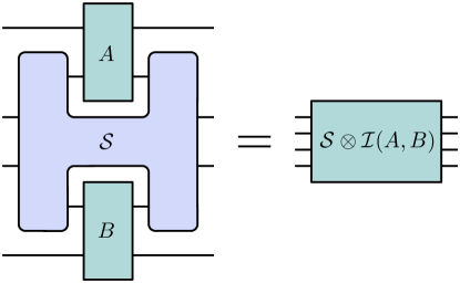
Figure 3: The extended quantum switch transformation. The quantum switch is a higher-order transformation that takes as input to quantum channels, $A$ and $B$, and transforms them into a different quantum channel, $\mathcal{S}\otimes\mathcal{I}(A,B)$, even when acting only on part of these channels.

We prove this result by explicitly constructing the quantum circuit that performs this simulation, which is given by

$$\quantikz[columnsep=3.8mm]&\ctrl{3}\ctrl{4}\ctrl{3}\ctrl{4}\ctrl[open]{3}\ctrl[open]{4}\ctrl[open]{3}\ctrl[open]{4}\\ \targX{}\targX{}\targX{}\targX{}\\ \targX{}\targX{}\targX{}\targX{}\\ \targX{}\gate[2,style={fill=JessicaColour!30},labelstyle=black]{A}\targX{}\targX{}\gate[2,style={fill=JessicaColour!30},labelstyle=black]{A}\targX{}\\ \targX{}\targX{}\gate[2,style={fill=JessicaColour!30},labelstyle=black]{B}\targX{}\targX{}\\ .$$ (9)

Here, the first circuit line represents the qubit control, the second and third lines represent auxiliary systems, the fourth line represents Alice’s primed system, the fifth line represents the target system, and the sixth line represents Bob’s primed system. In App. B.4, we prove Thm. 1 by explicitly writing the channel resulting from this circuit for all input channels $A$ and $B$, showing how it recovers that action of the quantum switch when $A$ is a unitary channel, and how it fails to recover the action of the quantum switch when $A$ is a general quantum channel.

II.4 No-go theorems: impossible simulations

We now show that the go-theorem from the previous section does not generalize: not only does the circuit in Eq. (8) does not work for arbitrary quantum channels $A$ and $B$, but there does not exist any quantum circuit that can simulate the quantum switch, even when an extra call of each input channel is available. In order to do so, we prove an even stronger statement. First, we define a restricted simulation of the quantum switch, which is a simulation of the action of the quantum switch that must hold only for a fixed choice of input systems and when the output target system is discarded. Then, we define probabilistic-heralded simulations of higher-order transformations. Finally, we show that when an extra call of each input channel is allowed, the maximum probability of simulating the quantum switch is always less than one, even for qubit channels in the restricted simulation scenario. The impossibility of simulating this particular case implies also the impossibility of simulation of the more general scenarios where the input systems are not fixed, the output target state is not discarded, the input channels act on higher-dimensional spaces, and when the quantum switch acts only on part of its input channels.

Let us start by defining the restricted simulation scenario. Fixing the input control system to be in state $\sigma_{c}=\outerproduct{+}{+}$ and the input target system to be in state $\rho_{t}=\outerproduct{0}{0}$, a restricted simulation of the switch is possible if, for some finite number of calls $k_{A}$ and $k_{B}$, there exists a higher-order transformation $\mathcal{C}$ that obeys causal constraints, such that

$$\begin{split}\tr_{t_{O}}\Big{(}\mathcal{C}(A^{\otimes k_{A}},\,B^{\otimes k_{B}})&[\,\outerproduct{+}{+}\otimes\outerproduct{0}{0}\,]\Big{)}\\ =\tr_{t_{O}}\Big{(}\mathcal{S}(A,B)&[\,\outerproduct{+}{+}\otimes\outerproduct{0}{0}\,]\Big{)}\ \ \ \forall\ A,B,\end{split}$$ (10)

where $A$ and $B$ are arbitrary channels. Notice that for every $A$ and $B$, Eq. (10) is an equality between two qubit quantum states, namely the output control systems. Notice that, while the impossibility of a simulation in the restricted case implies the impossibility of simulation in the general case, a possibility of simulating the quantum switch in the restricted case would not imply the existence of a more general simulation.

Let us now define a probabilistic heralded simulation of the quantum switch. A probabilistic heralded simulation can be described as a higher-order transformation that obeys causal constraints and which, compared to the deterministic simulation in Eq. (3), outputs an extra classical bit that corresponds to either a success or failure outcome of the simulation. When the value of this bit corresponds to the success outcome, the implemented simulation is exactly $\mathcal{S}(A,B)$. Such transformations can be implemented by either a quantum comb or as a QC-CC that additionally outputs a flag system that encodes the success or failure outcome, followed by a dichotomic quantum measurement of the flag system. Mathematically, a probabilistic heralded simulation is a higher-order transformation $\mathcal{C}=\mathcal{C}_{s}+\mathcal{C}_{f}$, where $\mathcal{C}_{s}$ and $\mathcal{C}_{f}$ are higher-order maps that completely preserve completely positive inputs—one associated to the success and the other with the failure outcome of the transformation—and where $\mathcal{C}$ is described as either a quantum comb or as a QC-CC. In this case, $\mathcal{C}=\mathcal{C}_{s}+\mathcal{C}_{f}$ is a probabilistic simulation of the quantum switch that uses $k_{A}$ calls of channel $A$ and $k_{B}$ calls of channel $B$ if it satisfies

$$\mathcal{C}_{s}(A^{\otimes k_{A}},B^{\otimes k_{B}})=p\,\mathcal{S}(A,B)\ \ \ \forall\ A,B,$$ (11)

where $A$ and $B$ are general quantum channels, and $p$ is the probability of a successful simulation, which is required to be independent of the inputs $A$ and $B$. In the case where $\mathcal{C}$ is a quantum comb, no normalization conditions need to be imposed on $\mathcal{C}_{s}$. However, when $\mathcal{C}$ is a QC-CC, then normalization conditions must be imposed on $\mathcal{C}_{s}$ to ensure that $\mathcal{C}$ is a proper QC-CC transformation [25]. We present these constraints explicitly in App. A.

Combining Eqs. (10) and (11), we define a probabilistic restricted simulation of the quantum switch via

$$\begin{split}\tr_{t_{O}}\Big{(}\mathcal{C}_{s}(A^{\otimes k_{A}},\,B^{\otimes k_{B}})&[\,\outerproduct{+}{+}\otimes\outerproduct{0}{0}\,]\Big{)}\\ =p\,\tr_{t_{O}}\Big{(}\mathcal{S}(A,B)&[\,\outerproduct{+}{+}\otimes\outerproduct{0}{0}\,]\Big{)}\ \ \ \forall\ A,B.\end{split}$$ (12)

It is known that any higher-order transformation with indefinite causal order can be simulated by a quantum comb in a probabilistic heralded manner with $p>0$, even without any extra calls of the input channels [22, 17]. For the particular case of the quantum switch, Ref. [6] presents a probabilistic circuit based on quantum teleportation that simulates the quantum switch with $p=1/d^{2}$, where $d$ is the dimension of the target system, without any extra calls. Here, we will analyse the maximal probability of success for simulating the quantum switch when extra calls are available, to show that, for certain numbers of extra calls, a deterministic simulation—i.e., one with a success probability of $p=1$—is not possible.

In any fixed dimension $d\coloneqq\dim(\mathcal{H}^{t_{I}})=\dim(\mathcal{H}^{t_{O}})=\dim(\mathcal{H}^{A_{I}})=\dim(\mathcal{H}^{A_{O}})=\dim(\mathcal{H}^{B_{I}})=\dim(\mathcal{H}^{B_{O}})$, there exist infinitely many quantum channels $A$ and $B$. However, determining the possibility of a simulation, as well as the highest probability of simulation, can be done by considering only a finite number of input quantum channels, due to the linearity of higher-order transformations. Furthermore, as we prove in Sec. IV, for any fixed finite $d$, $k_{A}$, and $k_{B}$, the maximum probability of success $p$ of simulating the quantum switch acting on all general quantum channels $A$ and $B$ can be computed with a semidefinite program (SDP). This is because if a simulation exists for a finite subset of channels that form a basis for the linear subspace spanned by $k_{A}$ copies of a quantum channel $A$, and equivalently for $B$, then said simulation is also valid for all channels $A$ and $B$. Crucially, in the case where $\mathcal{C}$ is a quantum comb, the maximum probability of success of a simulation of the quantum switch may depend on the order of the input channels $A$ and $B$. For example, in the case $(k_{A},k_{B})=(2,1)$, the possible orders AAB, ABA, and BAA must be considered. In the case where $\mathcal{C}$ is a QC-CC, all possible fixed and dynamical orders are automatically optimized over.

We are now ready to state our main theorem.

Theorem 2.

There does not exist a quantum circuit that can deterministically simulate the action of the quantum switch on all quantum channels when $(k_{A},k_{B})\in\{(1,1),(2,1),(2,2),(3,1)\}$, where $k_{A}$ is the number of calls of input channel $A$ and $k_{B}$ is the number of calls of input channel $B$.

Moreover, even for a restricted simulation—i.e., for fixed input systems and discarded output target system—the action on the quantum switch on qubit general channels, when $(k_{A},k_{B})\in\{(1,1),(2,1),(2,2),(3,1)\}$, can be simulated with at most a probability $p$ that is strictly less than one, with upper bounds given in Table 1.

We prove this theorem using a method that we develop for computer-assisted proofs that transforms the numerically imperfect solution of an SDP into a rigorous upper-bound for the probability of success that can be expressed in terms of rational numbers. The method is presented in Sec. IV with further details provided in App. E.

$(k_{A},k_{B})$	order	probability
$(1,1)$	AB	$p<\frac{4001}{10000}$
	AAB	$p<\frac{5715}{10000}$
$(2,1)$	ABA	$p<\frac{4919}{10000}$
	BAA	$p<\frac{5001}{10000}$
	AABB	$p<\frac{8307}{10000}$
$(2,2)$	ABAB	$p<\frac{8484}{10000}$
	ABBA	$p<\frac{8695}{10000}$
	AAAB	$p<\frac{8373}{10000}$
$(3,1)$	AABA	$p<\frac{6909}{10000}$
	ABAA	$p<\frac{7597}{10000}$
	BAAA	$p<\frac{6845}{10000}$

Table 1: Maximum probability of a restricted simulation of the qubit quantum switch. Upper bounds for the maximum probability of a restricted simulation of the quantum switch acting on a pair of arbitrary qubit quantum channels $A,B$, using quantum combs that act on $k_{A(B)}$ calls of an arbitrary quantum channel $A(B)$ in a certain order.

In the case of QC-CC simulations, due to limitations in computational power, we were not able to develop computer-assisted proofs of upper bounds for the probability of success. However, by numerically evaluating the SDPs for a QC-CC simulation in the cases of $(k_{A},k_{B})\in\{(1,1),(2,1)\}$, we observe that the maximum probability for a QC-CC simulation in the restricted qubit case is never higher than the maximum over quantum combs of all possible orders. In Sec. II.5, we show results related to QC-CCs in the approximate simulation scenario for these same values of $(k_{A},k_{B})$.

Still in the restricted simulation scenario, we found three different particular cases where a deterministic simulation is possible for qubit channels, but nevertheless impossible in more general scenario. In following we discuss these three cases, with more details being provided in App. C.

The first case of this kind is when the quantum switch acts on arbitrary, yet identical, qubit quantum channels, i.e., $A=B$. Although the input channels in this case are identical, it is straightforward to see from Eq. (1) that the action of the switch is non-trivial, namely, that the output channel $\mathcal{S}(A,A)$ is not equivalent to $A$ applied twice on the target system when $A$ is not a unitary channel. A remarkable example of this point is the case where $A$ is the depolarizing channel [26]. In the case of identical input channels, we find that a restricted deterministic simulation can be done with a quantum comb that requires one extra call of each input operation, amounting to $4$ identical calls of the arbitrary qubit quantum channel $A$, a scenario which we call AAAA. Since in this case the maximum probability of success is $p=1$, one cannot certify this result with a computer-assisted proof, which can yield upper and lower bounds for $p$ with arbitrary yet only finite precision. Instead, we obtain this result by numerically evaluating an SDP with very high precision, ensuring that all SDP positivity constraints are strictly satisfied and that all equality constraints are satisfied up to an error of at most $10^{-9}$ in the operator norm. Furthermore, $4$ identical calls of the arbitrary qubit quantum channel $A$ are not only sufficient, but necessary for a deterministic restricted simulation: if only $2$ or $3$ calls are allowed, we prove upper bounds for the maximum probability of simulation that are always strictly less than $1$. In Table 2 we present our results for identical qubit quantum channels. However, this result only holds in the restricted simulation case. When the output target system is not discarded, we find numerically that a deterministic simulation of the AAAA case is not possible. This shows how highly nontrivial the action of the quantum switch is even when acting on identical quantum channels.

$k$	order	probability
$2$	AA	$p<\frac{4001}{10000}$
$3$	AAA	$p<\frac{6534}{10000}$
$4$	AAAA	$p=1\ ({}^{*})$

Table 2: Bounds for the probability of a restricted simulation of the qubit quantum switch acting on identical channels. Upper bounds for the maximum probability of a restricted simulation of the quantum switch that acts on a pair of identical qubit quantum channels, using quantum combs that act on $k\in\{2,3\}$ calls of an arbitrary quantum channel $A$. (*) For the case of $k=4$, we numerically find that a deterministic simulation is possible, i.e., that $p=1$ up to an numerical precision of $10^{-9}$.

The other two restricted cases where a deterministic restricted simulation is possible concern qubit unitary channels. In particular, we find that a deterministic simulation is possible when qubit unitary channels are applied in the order AABB and BAAA, two cases where trivial extensions of the circuit in Eq. (6) fail. Similarly to the case of identical qubit channels, these simulations of qubit unitary channels also fail when the output target system is not discarded.

II.5 No-go theorems: robustness

By exhibiting concrete upper bounds for the probability of successful simulation of the quantum switch that are significantly below $1$, we demonstrate the extent of the robustness of our results with respect to a figure of merit related to a probabilistic simulation. Another pertinent notion of robustness in this context is that of an approximation simulation—although the quantum switch may not be able to be exactly simulated, it could still be the case that other higher-order transformations with indefinite causal order which are $\epsilon$-close to the quantum switch can be simulated. This question is particularly relevant for experimental scenarios, where noise and imprecision hinder the ability of preparing any specific transformation exactly. Here, we prove that even in the approximate case a simulation of the quantum switch is not possible, for some particular number of calls $(k_{A},k_{B})$. We do so by exhibiting values of $\epsilon$ that are significantly above $0$ for which even a probabilistic simulation, for some $p<1$ that we also exhibit, is not possible. In order to do so, we begin by defining approximate simulations.

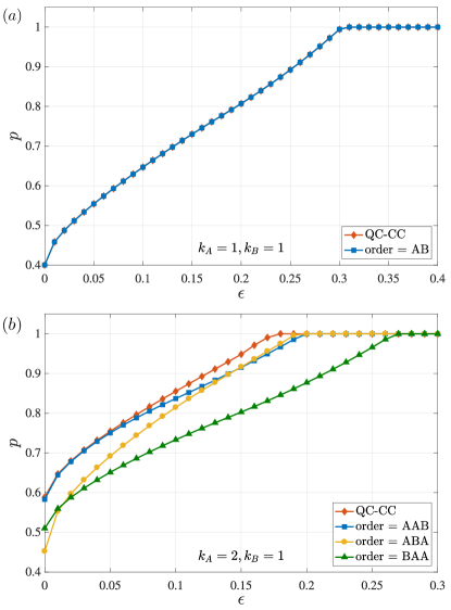
Figure 4: Robustness of the impossibility of simulation. Maximum probability of success of simulating any higher-order transformation that is $\epsilon$-close to the quantum switch using quantum combs of different orders or QC-CCs, as a function of $\epsilon$. In plot $(a)$, we show the case where $k_{A}=k_{B}=1$. Notice how the QC-CC simulation curve numerically coincides with the comb simulation curve. In plot $(b)$, we show the case where $k_{A}=2$ and $k_{B}=1$.

For an approximate simulation of the quantum switch, it is useful to consider a partly restricted kind of simulation that is required to hold for fixed input control and target systems, but without discarding the output target system. Similarly to the restricted simulation case, proving the impossibility of a simulation in this partly restricted case also implies the impossibility of a simulation in more general scenarios. Let $\sigma_{c}=\outerproduct{+}{+}$ be the state of the input control system, $\rho_{t}=\outerproduct{0}{0}$ be the state of the input target system, and $\widetilde{\mathcal{S}}$ be a higher-order transformation that acts on the same space as the quantum switch. We define a simulation $\mathcal{C}$ to be $\epsilon$-close to the quantum switch $\mathcal{S}$ in this scenario if there exists an $\widetilde{\mathcal{S}}$ such that

$$\begin{split}\mathcal{C}(A^{\otimes k_{A}},B^{\otimes k_{B}})&[\,\outerproduct{+}{+}\otimes\outerproduct{0}{0}\,]\\ =\widetilde{\mathcal{S}}(A,B)&[\,\outerproduct{+}{+}\otimes\outerproduct{0}{0}\,]\ \ \ \forall\ A,B,\end{split}$$ (13)

where $A$ and $B$ are arbitrary quantum channels and, for $\mathcal{S}_{+0}(\cdot,\cdot)\coloneqq\mathcal{S}(\cdot,\cdot)[\outerproduct{+}{+}\otimes\outerproduct{0}{0}]$ and $\widetilde{\mathcal{S}}_{+0}(\cdot,\cdot)\coloneqq\widetilde{\mathcal{S}}(\cdot,\cdot)[\outerproduct{+}{+}\otimes\outerproduct{0}{0}]$, it holds that

$$F(\mathcal{S}_{+0},\widetilde{\mathcal{S}}_{+0})\geq 1-\epsilon,$$ (14)

where $F(\mathcal{M},\mathcal{N})$ is the normalized fidelity between the Choi operators associated to the higher-order transformations $\mathcal{M}$ and $\mathcal{N}$ (see App. A).

Combining probabilistic-heralded and approximate protocols of simulation, for a fixed $\epsilon$, $(k_{A},k_{B})$, and $d$, the maximum probability of successful simulation can also be computed via an SDP. We show that, for a range of values of $\epsilon>0$, the probability of simulating the quantum switch in this partly restricted scenario is $p<1$ for the cases where $(k_{A},k_{B})\in\{(1,1),(2,1)\}$, considering simulations using quantum combs of all possible orders as well as QC-CCs. We present our numerical findings in Fig. 4 for the case where $d=2$. In the first plot [Fig. 4$(a)$], where $(k_{A},k_{B})=(1,1)$, the QC-CC simulation curve numerically coincides with the quantum comb simulation curve. In the second plot [Fig. 4$(b)$], where $(k_{A},k_{B})=(2,1)$, each of the three possible quantum comb orders and QC-CC yield different values for the maximum probability of success for different values of $\epsilon$. Notice that for an exact simulation, i.e., when $\epsilon=0$, a QC-CC simulation yields a probability of success that coincides with the highest among all possible orders, but as $\epsilon$ increases, it shows an advantage in the probability of success as compared to quantum combs.

III Discussion

In this work, we have concretely formulated the problem of simulating higher-order transformations with indefinite causal order using higher-order transformations that obey causal constraints and have access to more calls of the input operations. Our case study for this problem was the quantum switch. We defined the problem in its full generality, considering also cases where the quantum switch acts only on part of its input quantum channels, and discussed why naïve simulation attempts that are based on our intuition of quantum control of causal orders implemented with extra calls of the input channels fail.

We proved that an extra copy of each input quantum channel, i.e., $(k_{A},k_{B})=(2,2)$, is not sufficient to deterministically simulate the quantum switch with a quantum circuit. We also showed that two extra copies of one of the channels and no extra copies of the other, i.e., $(k_{A},k_{B})=(3,1)$, does not suffice. This case where only a single call of input channel $B$ is available has also been more generally addressed in our related work in Ref. [27]. There, we prove that when only a single call of channel $B$ is available ($k_{B}=1$), the quantum switch cannot be deterministically simulated by any QC-CC transformation whenever $k_{A}\leq\max\{2,2^{n}-1\}$, where $n$ is the number of qubits that the input channels act upon.

Additionally, we demonstrated how robust our results concerning impossibility of simulating the switch are: the switch cannot be simulated even approximately and for some probability $p<1$. We further showed that, for the particular case where the input pair of channels of the switch are identical qubit quantum channels, $4$ calls of the input channel are necessary and sufficient for a restricted deterministic simulation, where the input states are fixed and the target output system is discarded. However, this result does not hold for more general simulation scenarios, where the output target system is not discarded. This possibility of simulation in the restricted case, but not in more general cases, is also true for the simulation of the action of the switch on qubit unitary channels with the orders AABB and BAAA.

Our results have strong implications for the analysis of the experiments that have been and will be carried out based on the quantum switch, particularly the ones that make use of non-unitary channels, such as those reported in Refs. [28, 29, 30, 31, 32]. Although several experimental setups allow for the argument that there are two calls of each input quantum channel available in the transformation, we have proven here that such access still does not allow for a causal explanation for the observed data. Take as an example the experiment reported in Ref. [30], where a process tomography of the quantum switch was carried out. Our work implies that the data of this experiment is not compatible with any quantum circuit that acts on two calls of each input quantum channel. The data is, nevertheless, compatible with the quantum switch itself, up to experimental imprecision and under the device-dependent assumptions required by typical tomography procedures.

An alternative causal model that is able to explain the action of the quantum switch is one that, instead of considering the inputs to be two independent calls of a general channel, considers inputs that can be described as bipartite channels with memory, which implement what can be interpreted as two “correlated” uses of a general quantum channel [33, 34]. Although this model can reproduce the statistics of the quantum switch experiments, it is a corollary of our main result (Theorem 2) that there does not exist a quantum circuit which can take two independent uses of an arbitrary channel as input and output a bipartite channel with memory that corresponds to two correlated uses of the input quantum channels. Therefore, a causal model based on correlated inputs is not compatible with a simulation scenario that considers blackbox inputs, as considered here.

The question of whether any finite number of calls suffices to perform a simulation of the switch is of high relevance and remains open. Further investigation of this topic will be crucial to determine, for example, whether advantages in specific tasks that have been previously demonstrated can persist in the asymptotic limit of the available number of calls. Should it ever be shown that the quantum switch can be simulated with a finite number of calls, a relevant follow-up question is related to the scaling of the necessary number of calls, and to whether or not the switch can be efficiently simulated in a deterministic setting.

The existence of efficient deterministic and exact simulation of quantum processes with indefinite causal order may pose itself as an interesting physical guideline to help us understand on the one hand which kinds of higher-order transformations can be realistically implemented, and on the other hand, what advantages they may provide.

IV Methods

Semidefinite programming. Here we show that the problem of simulating the quantum switch can be phrased as an SDP. In order to do so, one needs to rewrite the problem using the Choi-Jamiołkowski isomorphism. Using this isomorphism, any linear map $\mathcal{M}:\mathcal{L}(\mathcal{H}^{I})\to\mathcal{L}(\mathcal{H}^{O})$ that maps linear operators acting on an input space to linear operators acting on an output space can be represented by a linear operator $M\in\mathcal{L}(\mathcal{H}^{I}\otimes\mathcal{H}^{O})$ that acts on the joint input and output space, called the Choi operator, which is given by $M\coloneqq\sum_{ij}\outerproduct{i}{j}\otimes\mathcal{M}(\outerproduct{i}{j})$, where $\{\ket{i}\}_{i}$ is the computational basis. A linear map $\mathcal{M}$ is completely positive (CP) if and only if its Choi operator $M$ is positive semidefinite, and is trace-preserving (TP) if and only if $M$ satisfies $\tr_{O}(M)=\mathbb{1}^{I}$. Using this representation, the composition of $\mathcal{G}\circ\mathcal{F}$ two maps $\mathcal{F}:\mathcal{L}(\mathcal{H}^{1})\to\mathcal{L}(\mathcal{H}^{2})$ and $\mathcal{G}:\mathcal{L}(\mathcal{H}^{2})\to\mathcal{L}(\mathcal{H}^{3})$, with respective Choi operators $F\in\mathcal{L}(\mathcal{H}^{1}\otimes\mathcal{H}^{2})$ and $G\in\mathcal{L}(\mathcal{H}^{2}\otimes\mathcal{H}^{3})$, is given by $F*G\in\mathcal{L}(\mathcal{H}^{1}\otimes\mathcal{H}^{3})$, with

$$F*G\coloneqq\tr_{2}[(F\otimes\mathbb{1}^{3})(\mathbb{1}^{1}\otimes G^{T_{2}})],$$ (15)

where $(\cdot)^{T_{X}}$ denotes partial transposition on the space $\mathcal{L}(\mathcal{H}^{X})$. The operation $*$ is called the link product [1].

Let $S$ be the Choi operator of the quantum switch transformation $\mathcal{S}$, defined in Eq. (1), written explicitly in App. A. Let $J^{A}$ and $J^{B}$ be the Choi operators of the quantum channels $A$ and $B$. Finally, let $C$ be the Choi operator of the deterministic higher-order transformation $\mathcal{C}$, which corresponds to a quantum comb, and $C_{s}$ be the Choi operator of the higher-order transformation $\mathcal{C}_{s}$ associated with the success outcome of a probabilistic transformation. Then, the maximum probability of simulating the action of the quantum switch $S$ on a set of $N_{A}$ channels $\{J^{A}_{i}\}_{i=1}^{N_{A}}$ and a set of $N_{B}$ channels $\{J^{B}_{j}\}_{j=1}^{N_{B}}$ using a quantum comb $C$ that acts on $k_{A}$ calls of $J^{A}_{i}$ and $k_{B}$ calls of $J^{B}_{j}$ is given by the following SDP:

$$\begin{aligned} \textbf{given}\ \ &\{J^{A}_{i}\}_{i},\{J^{B}_{j}\}_{j},k_{A},k_{B}\\ \textbf{max}\ \ &p\\ \textbf{s.t.}\ \ &C_{s}*[{(J^{A}_{i})}^{\otimes k_{A}}\otimes{(J^{B}_{j})}^{\otimes k_{B}}]=p\,S*(J^{A}_{i}\otimes J^{B}_{j})\ \ \forall\,i,j\\ &C_{s}\geq 0,\ \ C-C_{s}\geq 0,\\ &\mathbb{P}(C)=C,\ \ \tr(C)=d_{c_{I}}d_{t_{I}}d_{A_{O}}^{k_{A}}d_{B_{O}}^{k_{B}},\end{aligned}$$ (16)

where $\mathbb{P}$ is the projector onto the linear subspace spanned by valid quantum combs [1, 8, 5] (explicitly written in App. A), and $d_{X}\coloneqq\text{dim}(\mathcal{H}^{X})$. For a simulation given by QC-CC transformations, the constraint $\mathbb{P}(C)=C$ should be substituted by the appropriate linear constraints that define a proper QC-CC transformations, as well as additional normalization constraints on $C_{s}$ [25]. These constraints are explicitly written in App. A for the cases of $2$ and $3$ slots. Notice that, following results from Sec. III of Ref. [17], the variables $C$ and $C_{s}$ in this SDP can be restricted to the field of real numbers without loss of generality, a feature that improves numerical performance.

The dual problem associated to this SDP can be found by combining standard methods [35] with dual affine techniques (see, e.g., the derivation of a similar dual problem in Appendix B of Ref. [10], inspired by Ref. [36]). It is given by

$$\begin{aligned} \textbf{given}\ \ &\{J^{A}_{i}\}_{i},\{J^{B}_{j}\}_{j},k_{A},k_{B}\\ \textbf{min}\ \ &\frac{1}{d_{A_{I}}^{k_{A}}d_{B_{I}}^{k_{B}}d_{c_{O}}d_{t_{O}}}\tr(\Gamma)\\ \textbf{s.t.}\ \ &\sum_{i,j}\tr[R_{ij}\,(S*(J^{A}_{i}\otimes J^{B}_{j}))]=1\\ &\Gamma-\sum_{i,j}R_{ij}\otimes[{(J^{A}_{i})}^{\otimes k_{A}}\otimes{(J^{B}_{j})}^{\otimes k_{B}}]^{T}\geq 0\\ &\Gamma\geq 0,\ \ \overline{\mathbb{P}}(\Gamma)=\Gamma,\end{aligned}$$ (17)

where $\overline{\mathbb{P}}$ is the projector onto the linear subspace spanned by the dual affine of valid combs [36, 10, 5] (also explicitly written in App. A). In the case of this dual SDP problem, the variable $\Gamma$ may also be restricted to the field of real numbers, since it is the Lagrange multiplier associated to the constraint $\mathbb{P}(C)=C$ (an equality between real matrices); however, the same is not true for the variables $\{R_{ij}\}$, which are the Lagrange multipliers associated to the constraints $C_{s}*[{(J^{A}_{i})}^{\otimes k_{A}}\otimes{(J^{B}_{j})}^{\otimes k_{B}}]=p\,S*(J^{A}_{i}\otimes J^{B}_{j})$, an equality between complex matrices. Nonetheless, restricting $\{R_{ij}\}$ to real values still allows for feasible points that yield a valid upper bound for the optimal solution of this problem.

Finally, the SDPs (16) and (17) satisfy the condition of strong duality, which is implied by the fact that a strictly feasible point for the primal problem can be created from the probabilistic simulation of Ref. [6] that requires no extra calls.

Basis design. For any input set of channels, the solution of SDP (16), or equivalently of SDP (17), corresponds to the maximum probability of success of a simulation of the action of the quantum switch on the specific given inputs, with a simulation that has access to the specified number of calls of the input channels and that satisfies the specified causal constraints. Then, the maximum probability of success of a universal switch simulation—one that works for all possible input channels and not only for the given inputs—can be obtained by setting $\{{(J^{A}_{i})}\}_{i}$ to be a set of operators that forms a basis for the $\text{span}(\{(J^{A}_{i})^{\otimes k_{A}}\}_{i})$, i.e., the subspace spanned by $k_{A}$ copies of an arbitrary quantum channel, and equivalently for $\{{(J^{B}_{i})}\}$. In this case, if the constraint $C_{s}*[{(J^{A}_{i})}^{\otimes k_{A}}\otimes{(J^{B}_{j})}^{\otimes k_{B}}]=p\,S*(J^{A}_{i}\otimes J^{B}_{j})$ holds for all $i,j$, then it also holds for arbitrary quantum channels. In other words, it implies that $C_{s}*[{(J^{A})}^{\otimes k_{A}}\otimes{(J^{B})}^{\otimes k_{B}}]=p\,S*(J^{A}\otimes J^{B})$ holds for all channels $J^{A}$ and $J^{B}$, thereby implying the existence of a universal probabilistic simulator with success probability $p$.

There are a few properties that the elements $J^{A}_{i}$ and $J^{B}_{j}$ of these bases must satisfy in order to be valid inputs of the SDPs (16) and (17). The first is that it is necessary to ensure that the operators $J^{A}_{i}$ and $J^{B}_{j}$ individually correspond to TP maps, in order for the total trace of both sides of the constraint $C_{s}*[{(J^{A}_{i})}^{\otimes k_{A}}\otimes{(J^{B}_{i})}^{\otimes k_{B}}]=p\,S*(J^{A}_{i}\otimes J^{B}_{i})$ to match. However, they do not need to correspond to CP maps, i.e., to be positive semidefinite operators. That is because all elements of the $\text{span}(\{J^{A}_{i}\}_{i})$ can be written as linear combinations of the elements of a set $\{{J^{\prime}}^{A}_{i}\}_{i}$ which correspond to TP maps (but not necessarily CP maps) and form a basis for the space spanned by quantum channels. Finally, it is also necessary that these operators can be themselves expressed as a tensor power of a TP map, because they play the role of the inputs of the quantum switch, which takes only a single call of each input. That is, they appear on both sides of the constraint $C_{s}*[{(J^{\prime A}_{i})}^{\otimes k_{A}}\otimes{(J^{\prime B}_{j})}^{\otimes k_{B}}]=p\,S*(J^{\prime A}_{i}\otimes J^{\prime B}_{j})$.

We now construct a convenient basis for the linear space spanned by the set of $k$ copies of any quantum channel, which will be used in the computer-assisted proofs presented subsequently.

First, note that an arbitrary self-adjoint two-qubit operator $M\in\mathcal{L}(\mathcal{H}^{I}\otimes\mathcal{H}^{O})\cong\mathcal{L}(\mathbb{C}^{2}\otimes\mathbb{C}^{2})$ can always be written as

$$\begin{split}M=\,&\lambda\,\mathbb{1}\otimes\mathbb{1}\\ &+\sum_{i}\alpha_{i}\,\sigma_{i}\otimes\mathbb{1}+\sum_{j}\beta_{j}\,\mathbb{1}\otimes\sigma_{j}+\sum_{ij}\gamma_{ij}\sigma_{i}\otimes\sigma_{j},\end{split}$$ (18)

where all $\sigma_{i}\in\{X,Y,Z\}$ are Pauli operators, and $\lambda,\alpha_{i},\beta_{j},\gamma_{ij}\in\mathbb{R}$. Since operators $M$ that correspond to a TP map satisfy $\tr_{O}(M)=\mathbb{1}^{I}$, in this case one has that $\lambda=1/2$ and $\alpha_{i}=0$. This implies that the dimension of the linear space spanned by the set of qubit quantum channels is $3+9+1=13$. One can then construct a convenient basis for the subspace spanned by qubit quantum channels, given by

$$\begin{split}\mathcal{B}_{1}\coloneqq\Big{\{}&\mathbb{1}\otimes\frac{\mathbb{1}}{2},\\ &\mathbb{1}\otimes\frac{\mathbb{1}}{2}+\mathbb{1}\otimes\sigma_{i},\\ &\mathbb{1}\otimes\frac{\mathbb{1}}{2}+\sigma_{j}\otimes\sigma_{k}\Big{\}}_{i,j,k}.\end{split}$$ (19)

Notice that all elements of the basis set $\mathcal{B}_{1}$ correspond to TP maps, even if they are not necessarily positive semidefinite.

We now consider the linear space spanned by the set of $k$ copies of any arbitrary qubit channel, i.e., the span of the set of all ${J}^{\otimes k}$ such that $\tr_{O}(J)=\mathbb{1}^{I}$. If a linear subspace $\mathcal{V}$ has dimension $d_{\mathcal{V}}$, then the dimension of the space $\text{span}(\{{J}^{\otimes k}|\,{J}^{\otimes k}\in\mathcal{V}\})$ is given by $\binom{d_{\mathcal{V}}-1+k}{k}$ [24]. By setting $d_{\mathcal{V}}=13$ and $k=2$, we see that the space spanned by the set of two identical copies of qubit channels has dimension $91$. Hence, in order to find a basis for two identical copies of qubit channels, it is enough to exhibit a set of $91$ operators $J_{i}$, all respecting $\tr_{O}(J_{i})=\mathbb{1}^{I}$, such that the set $\{{J_{i}}^{\otimes 2}\}_{i=1}^{91}$ is composed of linearly independent operators.

Let $\rho_{i}\in\{\mathbb{1}\otimes\frac{\mathbb{1}}{2},2\outerproduct{\phi^{+}}{\phi^{+}},\mathbb{1}\otimes\outerproduct{0}{0},\mathbb{1}\otimes\outerproduct{+}{+},\mathbb{1}\otimes\outerproduct{+_{Y}}{+_{Y}}\}$, where $\ket{\phi^{\pm}}\coloneqq\frac{1}{\sqrt{2}}(\ket{00}\pm\ket{11})$ are maximally entangled two-qubit states and $\ket{\pm_{Y}}\coloneqq\frac{1}{\sqrt{2}}(\ket{0}\pm i\ket{1})$. Then, let $\sigma^{I}_{i}\in\{\mathbb{1},X,Y,Z\}$ and $\sigma^{O}_{i}\in\{X,Y,Z\}$. We define the set of operators

$$\begin{split}\mathcal{B}_{2}\coloneqq\Big{\{}&\Big{(}\mathbb{1}\otimes\frac{\mathbb{1}}{2}\Big{)}^{\otimes 2},\\ &\big{(}\rho_{i}\pm\sigma^{I}_{j}\otimes\sigma^{O}_{k}\big{)}^{\otimes 2},\\ &\big{(}\rho_{l}+\sigma^{I}_{m}\otimes\sigma^{O}_{n}+\sigma^{I}_{p}\otimes\sigma^{O}_{q}\big{)}^{\otimes 2}\Big{\}}_{\begin{subarray}{c}i,j,k,l,\\ m,n,p,q\end{subarray}},\end{split}$$ (20)

which can be shown to contain a subset of $91$ linearly independent operators by standard computational methods. Hence, the set $\mathcal{B}_{2}$ forms an “overcomplete” basis, from which one can obtain a standard basis (containing only $91$ operators) by discarding any operators that are not linearly independent. This set of $91$ operators forms a basis for the linear subspace spanned by two identical copies of any arbitrary qubit channel.

For the case of $k=3$, we begin by calculating the dimension of the space spanned by three identical copies of arbitrary qubit channels, by setting $d_{\mathcal{V}}=13$ and $k=3$, obtaining that the dimension of the relevant space is $455$. Again, in order to find a basis for three identical copies of qubit channels, it is enough to exhibit $455$ operators $J_{i}$ respecting $\tr_{O}(J_{i})=\mathbb{1}^{I}$, such that such that the set $\{{J_{i}}^{\otimes 3}\}_{i=1}^{455}$ is composed of linearly independent operators.

Let $\rho_{i}\in\{\mathbb{1}\otimes\frac{\mathbb{1}}{2},2\outerproduct{\phi^{+}}{\phi^{+}},2\outerproduct{\phi^{-}}{\phi^{-}},2\outerproduct{\psi^{+}}{\psi^{+}},$ $2\outerproduct{\psi^{-}}{\psi^{-}},\mathbb{1}\otimes\outerproduct{0}{0},\mathbb{1}\otimes\outerproduct{1}{1},\mathbb{1}\otimes\outerproduct{+}{+},\mathbb{1}\otimes\outerproduct{-}{-},\mathbb{1}\otimes\outerproduct{+_{Y}}{+_{Y}}\},\mathbb{1}\otimes\outerproduct{-_{i}}{-_{i}}\}$, where $\ket{\psi^{\pm}}\coloneqq\frac{1}{\sqrt{2}}(\ket{01}\pm\ket{10})$ are maximally entangled two-qubit states and $\ket{-}\coloneqq\frac{1}{\sqrt{2}}(\ket{0}-\ket{1})$. Then, let $\sigma^{I}_{i}\in\{\mathbb{1},X,Y,Z,X+Z,X+Y\}$ and $\sigma^{O}_{i}\in\{X,Y,Z,X+Z,X+Y\}$. We define the set of operators

$$\begin{split}\mathcal{B}_{3}\coloneqq\Big{\{}&\big{(}\rho_{i}\pm\sigma^{I}_{j}\otimes\sigma^{O}_{k}+\sigma^{I}_{l}\otimes\sigma^{O}_{m}\big{)}^{\otimes 3}\Big{\}}_{\begin{subarray}{c}i,j,k,\\ l,m\end{subarray}},\end{split}$$ (21)

which can be shown to contain a subset of $455$ linearly independent operators by standard computational methods. This set of $455$ operators forms a basis for the linear subspace spanned by three identical copies of arbitrary qubit channels.

In general, one can always construct a basis for the space spanned by $k\in\mathbb{N}$ copies of arbitrary qubit channels by finding coefficients $\alpha_{i|l},\gamma_{ij|l}\in\mathbb{R}$, such that the set

$$\left\{\left(\mathbb{1}\otimes\frac{\mathbb{1}}{2}+\sum_{i}\alpha_{i|l}\,\mathbb{1}\otimes\sigma_{i}+\sum_{ij}\gamma_{ij|l}\,\sigma_{i}\otimes\sigma_{j}\right)^{\otimes k}\right\}_{l}$$ (22)

contains $\binom{13-1+k}{k}$ linearly independent operators. One simple way to find such coefficients is simply to choose them at random.

To evaluate the SDPs (16) and (17) when the inputs form a basis for the space spanned by $k_{A}$ copies of channel $A$ and $k_{B}$ copies of channel $B$, the overall number of input pairs of channels are: for $(k_{A},k_{B})=(1,1)$, $N_{A}N_{B}=13\cdot 13=169$; for $(k_{A},k_{B})=(2,1)$, $N_{A}N_{B}=91\cdot 13=1183$; for $(k_{A},k_{B})=(3,1)$, $N_{A}N_{B}=455\cdot 13=5915$; and finally for $(k_{A},k_{B})=(2,2)$, $N_{A}N_{B}=91\cdot 91=8281$, making these SDPs very computationally demanding.

Computer-assisted proofs. While floating-point arithmetic provides an efficient and powerful numerical method to treat real numbers, it suffers from some fundamentally unavoidable issues. For instance, addition and multiplication of floats is not associative and equality and inequality constraints are not satisfied exactly, but only up to some numerical precision. We now show how efficient numerical solvers that make use of floating-point arithmetic can be used to obtain a rigorous upper bound on the maximal success probability of simulating the quantum switch, hence leading to a bona-fide computer-assisted proof. Our methods are based on Ref. [10].

The duality aspects of semidefinite programming [35] ensure that any feasible point of the dual problem, presented in SDP (17), yields an upper bound for the solution of the maximisation problem in the primal SDP (16). That is, any set of operators $\{R_{ij}\}_{ij}$ and $\Gamma$ that respects $\sum_{i,j}\tr[R_{ij}\,(S*(J^{A}_{i}\otimes J^{B}_{j}))]=1$, $\Gamma-\sum_{i,j}R_{ij}\otimes[{(J^{A}_{i})}^{\otimes k_{A}}\otimes{(J^{B}_{j})}^{\otimes k_{B}}]^{T}\geq 0$, $\Gamma\geq 0$, and $\overline{\mathbb{P}}(\Gamma)=\Gamma$, implies that the probability of simulating the quantum switch is necessarily $p\leq\tr(\Gamma)/d_{c_{I}}d_{t_{I}}d_{A_{O}}^{k_{A}}d_{B_{O}}^{k_{B}}$. Standard numerical SDP solvers can be used to find a floating-point solution for the dual problem in SDP (17), and to provide explicit operators $\{R_{ij}^{\texttt{float}}\}_{ij}$ and $\Gamma^{\texttt{float}}$ that approximately satisfy the SDP constraints. We now show how the operators $\{R_{ij}^{\texttt{float}}\}_{ij}$ and $\Gamma^{\texttt{float}}$ can be used as a good initial ansatz to construct symbolic operators $R_{ij}^{\texttt{OK}}$ and $\Gamma^{\texttt{OK}}$, which are not stored as floating-point variables and which satisfy the SDP constraints exactly, ensuring that $\tr(\Gamma^{\texttt{OK}})/d_{c_{I}}d_{t_{I}}d_{A_{O}}^{k_{A}}d_{B_{O}}^{k_{B}}$ is a legitimate upper bound for the probability of success of simulating the quantum switch. In order to do so, we use the bases presented in Eqs. (19), (20), (21), and (22), which only contain small rational numbers. In the following, we present an algorithm to extract a computer-assisted proof from numerical solvers.

Algorithm:

1. Construct symbolic non-floating-point operators $\Gamma^{\texttt{sym}}$ and $R_{ij}^{\texttt{sym}}$ by truncating $\Gamma^{\texttt{float}}$ and $R_{ij}^{\texttt{float}}$ to obtain symbolic operators expressed only in terms of rational numbers.
   This allows us to work with fractions and to avoid numerical imprecision.

2. Force the operators $\Gamma^{\texttt{sym}}$ and $R_{ij}^{\texttt{sym}}$ to be self-adjoint by making use of the expression ${(M+M^{\dagger})/2}$, which is self-adjoint for any $M$.
   This ensures that we are dealing with self-adjoint operators.

3. Evaluate ${t^{\texttt{sym}}\coloneqq\sum_{i,j}\tr[R^{\texttt{sym}}_{ij}\,(S*(J^{A}_{i}\otimes J^{B}_{j}))]}$, where $S,J^{A}_{i},$ and $J_{j}^{B}$ are also symbolic operators. Define $R_{ij}^{\texttt{OK}}\coloneqq R^{\texttt{sym}}_{ij}/t^{\texttt{sym}}$ for all $i,j$.
   Here, we use the basis with rational coefficients constructed earlier to ensure that the operators $R_{ij}^{\texttt{OK}}$ satisfy the SDP equality constraint exactly.

4. Project $\Gamma^{\texttt{sym}}$ onto the appropriate subspace to obtain $\overline{\mathbb{P}}(\Gamma^{\texttt{sym}})$.
   This ensures that the resulting operator $\overline{\mathbb{P}}(\Gamma^{\texttt{sym}})$ is in the correct linear subspace.

5. Find $\eta\in\mathbb{R}$ such that $\Gamma^{\texttt{OK}}\coloneqq\overline{\mathbb{P}}(\Gamma^{\texttt{sym}})+\eta\mathbb{1}\geq 0$ and $\Gamma^{\texttt{OK}}-\sum_{i,j}R_{ij}^{\texttt{OK}}\otimes({J^{A}_{i}}^{\otimes k_{A}}\otimes{J^{B}_{j}}^{\otimes k_{B}})^{T}\geq 0$
   This ensures the positivity constraints in the dual SDP (17) are satisfied.

6. Output the quantity $\tr(\Gamma^{\texttt{OK}})/d_{c_{I}}d_{t_{I}}d_{A_{O}}^{k_{A}}d_{B_{O}}^{k_{B}}$, which is a rigorous upper bound of the primal problem.
   All equality and inequality constraints hold without relying on floating point precision, and the operators $\Gamma^{\texttt{OK}}$ and $R_{ij}^{\texttt{OK}}$ yield a proof certificate that $p\leq\tr(\Gamma^{\texttt{OK}})/d_{c_{I}}d_{t_{I}}d_{A_{O}}^{k_{A}}d_{B_{O}}^{k_{B}}$.

The algorithm described above deserves two clarifications. First, since the projector $\overline{\mathbb{P}}$ is unital, i.e., $\overline{\mathbb{P}}(\mathbb{1})=\mathbb{1}$, for any $\eta\in\mathbb{R}$ and any operator $M$, we have that $\overline{\mathbb{P}}(M)+\eta\mathbb{1}=\overline{\mathbb{P}}(M+\eta\mathbb{1})$. Second, checking if an operator is positive semidefinite can be done efficiently through the Cholesky decomposition [37]—more details are provided in App. E.

Code availability. All code developed for this work is available at our online repository in Ref. [38]. For numerically evaluating all SDPs involving $4$-slot quantum combs and $3$-slot QC-CCs, we used the Splitting Conic Solver (SCS) [39, 40]. For all others, we used MOSEK [41].

Acknowledgements. We are grateful to Alastair Abbott and Cyril Branciard for interesting discussions about simulations of indefinite causal order, and to Denis Rosset and Siegfried M. Rump for helpful discussions regarding computer-assisted proofs. JB acknowledges funding from the Swiss National Science Foundation (SNSF) through the funding schemes SPF and NCCR SwissMAP. SY acknowledges support by Japan Society for the Promotion of Science (JSPS) KAKENHI Grant Number 23KJ0734, FoPM, WINGS Program, the University of Tokyo, and DAIKIN Fellowship Program, the University of Tokyo. PT acknowledges funding from the Japan Society for the Promotion of Science (JSPS) Postdoctoral Fellowships for Research in Japan. This work was supported by the MEXT Quantum Leap Flagship Program (MEXT QLEAP) JPMXS0118069605, JPMXS0120351339, the Japan Society for the Promotion of Science (JSPS) KAKENHI Grant Number 21H03394 and 23K21643, and IBM Quantum. We acknowledge the Japanese-French Laboratory for Informatics (JFLI) for the support on organising the Japanese-French Quantum Information 2023 workshop. Research at Perimeter Institute is supported in part by the Government of Canada through the Department of Innovation, Science and Economic Development and by the Province of Ontario through the Ministry of Colleges and Universities.

APPENDIX

The appendix is organized in the following way:

• Appendix A: Definitions and Choi operators

  • A.1. The quantum switch Choi operator and Choi operator fidelity

  • A.2. Quantum combs, probabilistic quantum combs, and projectors

  • A.3. QC-CCs and probabilistic QC-CCs

• Appendix B: General simulation scenarios

  • B.1. The action of the quantum switch on bipartite quantum channels

  • B.2. The action of the quantum switch on quantum instruments

  • B.3. The relationship with Stinespring dilation of quantum channels

  • B.4. Theorem 1: A simulation for bipartite unitary channels $U_{A}$ and bipartite general channels $B$

• Appendix C: Possible restricted simulations for qubit channels

• Appendix D: No-go results for unitary channels

• Appendix E: Efficient certification that a matrix is positive semidefinite

Appendix A Definitions and Choi operators

In this section, we explicitly define the key higher-order transformations used in the main text in terms of their Choi operators, which are crucial for the SDP implementation of our methods.

A.1 The quantum switch Choi operator and Choi operator fidelity

We begin with the Choi operator of the quantum switch transformation [8]. The quantum switch higher-order transformation $\mathcal{S}$ defined in Eq. (1) can be equivalently expressed by its associated Choi operator $S\in\mathcal{L}(\mathcal{H}^{c_{I}}\otimes\mathcal{H}^{t_{I}}\otimes\mathcal{H}^{A_{I}}\otimes\mathcal{H}^{A_{O}}\otimes\mathcal{H}^{B_{I}}\otimes\mathcal{H}^{B_{O}}\otimes\mathcal{H}^{t_{O}}\otimes\mathcal{H}^{c_{O}})$. Let the vector $\ket{s}$ be defined as

$$\ket{s}\coloneqq\ket{0}^{c_{I}}\ket{\mathbb{1}}^{t_{I}A_{I}}\ket{\mathbb{1}}^{A_{O}B_{I}}\ket{\mathbb{1}}^{B_{O}t_{O}}\ket{0}^{c_{O}}+\ket{1}^{c_{I}}\ket{\mathbb{1}}^{t_{I}B_{I}}\ket{\mathbb{1}}^{B_{O}A_{I}}\ket{\mathbb{1}}^{A_{O}t_{O}}\ket{1}^{c_{O}},$$ (23)

where $\ket{\mathbb{1}}^{XY}\coloneqq\sum_{i}\ket{i}^{X}\ket{i}^{Y}$ is the vector related to the Choi operator $\outerproduct{\mathbb{1}}{\mathbb{1}}$ of an identity channel from space $X$ to $Y$. Then, the Choi operator of the quantum switch is defined as

$$S\coloneqq\outerproduct{s}{s}.$$ (24)

This is the operator $S$ that appears in the first constraint of the SDPs (16) and (17).

The Choi operator of the quantum channel $\mathcal{S}(A,B)$ that results from the action of the quantum switch transformation $\mathcal{S}$ on input channels $A$ and $B$ can be expressed in terms of their respective Choi operators $S$, $J^{A}$, and $J^{B}$, as $S*(J^{A}\otimes J^{B})\in\mathcal{L}(\mathcal{H}^{c_{I}}\otimes\mathcal{H}^{t_{I}}\otimes\mathcal{H}^{t_{O}}\otimes\mathcal{H}^{c_{O}})$, where $*$ is the link product defined in Sec. IV.

In the case considered in the main text where the quantum switch has a fixed input state for its control and target systems, respectively given by $\sigma_{c}=\outerproduct{+}{+}\in\mathcal{L}(\mathcal{H}^{c_{I}})$ and $\rho_{t}=\outerproduct{0}{0}\in\mathcal{L}(\mathcal{H}^{t_{I}})$, we defined the resulting transformation as $\mathcal{S}_{+0}(\cdot,\cdot)\coloneqq\mathcal{S}(\cdot,\cdot)[\outerproduct{+}{+}\otimes\outerproduct{0}{0}]$. This higher-order operation has an associated Choi operator $S_{+0}\in\mathcal{L}(\mathcal{H}^{A_{I}}\otimes\mathcal{H}^{A_{O}}\otimes\mathcal{H}^{B_{I}}\otimes\mathcal{H}^{B_{O}}\otimes\mathcal{H}^{t_{O}}\otimes\mathcal{H}^{c_{O}})$ given by

$$S_{+0}\coloneqq \Big{(}\outerproduct{+}{+}\otimes\outerproduct{0}{0}\Big{)}*S$$ (25)

$$= \outerproduct{s_{+0}}{s_{+0}},$$ (26)

where

$$\ket{s_{+0}}\coloneqq\Big{(}\bra{+}^{c_{I}}\bra{0}^{t_{I}}\otimes\mathbb{1}\Big{)}\ket{s}=\frac{1}{\sqrt{2}}\Big{(}\ket{0}^{A_{I}}\ket{\mathbb{1}}^{A_{O}B_{I}}\ket{\mathbb{1}}^{B_{O}t_{O}}\ket{0}^{c_{O}}+\ket{1}^{B_{I}}\ket{\mathbb{1}}^{B_{O}A_{I}}\ket{\mathbb{1}}^{A_{O}t_{O}}\ket{1}^{c_{O}}\Big{)}.$$ (27)

We now define the Choi operator fidelity. Let $\widetilde{\mathcal{S}}$ be a higher-order transformation that acts on the same spaces as the quantum switch $\mathcal{S}$, and let $\widetilde{\mathcal{S}}_{+0}\coloneqq\widetilde{\mathcal{S}}(\cdot,\cdot)[\outerproduct{+}{+}\otimes\outerproduct{0}{0}]$ be $\widetilde{\mathcal{S}}$ with fixed input states for its control and target systems. The Choi operator fidelity between $\mathcal{S}_{+0}$ and any higher-order operation $\widetilde{\mathcal{S}}_{+0}$, with Choi operator $\widetilde{S}_{+0}$ is given by

$$F(\mathcal{S}_{+0},\widetilde{\mathcal{S}}_{+0})\coloneqq\frac{1}{(d_{A_{O}}d_{B_{O}})^{2}}\tr(S_{+0}\,\widetilde{S}_{+0})=\frac{1}{(d_{A_{O}}d_{B_{O}})^{2}}\Big{|}\bra{s_{+0}}\widetilde{\mathcal{S}}_{+0}\ket{s_{+0}}\Big{|},$$ (28)

where the factor $d_{A_{O}}d_{B_{O}}=\tr(S_{+0})=\tr(\widetilde{S}_{+0})$ ensures that $F(\mathcal{S}_{+0},\widetilde{\mathcal{S}}_{+0})\in[0,1]$.

A.2 Quantum combs, probabilistic quantum combs, and projectors

A probabilistic quantum comb is a quantum comb that yields a classical output with a certain probability. In our case, we consider probabilistic quantum combs that have two possible classical outcomes, success or failure. We recall that such transformations can be implemented by a quantum comb that additionally output a flag system that encodes the success or failure outcome, followed by a dichotomic quantum measurement of the flag system. In the case of a quantum comb $\mathcal{C}=\mathcal{C}_{s}+\mathcal{C}_{f}$ that performs a probabilistic simulation of the quantum switch, its associated Choi operator is given by $C=C_{s}+C_{f}$, where $C,C_{s},C_{f}\in\mathcal{L}(\mathcal{H}^{c_{I}}\otimes\mathcal{H}^{t_{I}}\otimes(\mathcal{H}^{A_{I}}\otimes\mathcal{H}^{A_{O}})^{\otimes k_{A}}\otimes(\mathcal{H}^{B_{I}}\otimes\mathcal{H}^{B_{O}})^{\otimes k_{B}}\otimes\mathcal{H}^{t_{O}}\otimes\mathcal{H}^{c_{O}})$. These operators are characterised by

$$C_{s} \geq 0$$ (29)

$$C_{f}=C-C_{s} \geq 0$$ (30)

$$\tr(C) =d_{c_{I}}d_{t_{I}}d_{A_{O}}^{k_{A}}d_{B_{O}}^{k_{B}}$$ (31)

$$C =\mathbb{P}_{k}(C),$$ (32)

where $k=k_{A}+k_{B}$ is the total number of slots in the quantum comb $C$, and $\mathbb{P}_{k}$ is the projector onto the subspace spanned by $k$-slot quantum combs.

The projector $\mathbb{P}_{k}$ is defined in full generality in Ref. [5]. For sake of completeness, we explicitly write $\mathbb{P}_{k}$ here in the cases where $k\in\{2,3,4\}$, which are the ones involved in our numerical calculations. To simplify the notation in the definition of the projector, let us define a $k$-slot quantum comb by its Choi operator $C\in\mathcal{L}(\mathcal{H}^{P}\otimes\mathcal{H}^{I_{1}}\otimes\mathcal{H}^{O_{1}}\otimes\ldots\otimes\mathcal{H}^{I_{k}}\otimes\mathcal{H}^{O_{k}}\otimes\mathcal{H}^{F})$. Then, let us define the trace-and-replace operation acting on the subspace $\mathcal{H}^{X}$ of an operator $C$ as

$${}_{X}C\coloneqq\tr_{X}(C)\otimes\frac{\mathbb{1}^{C}}{d_{C}}.$$ (33)

We are now ready to explicitly write the projector $\mathbb{P}_{k}$ for $k\in\{2,3,4\}$. For the case where $k=2$,

$$\mathbb{P}_{2}(C)=\,C-\,_{F}C+\,_{O_{2}F}C-\,_{I_{2}O_{2}F}C+\,_{O_{1}I_{2}O_{2}F}C-\,_{I_{1}O_{1}I_{2}O_{2}F}C+\,_{PI_{1}O_{1}I_{2}O_{2}F}C.$$ (34)

For the case where $k=3$,

$$\begin{split}\mathbb{P}_{3}(C)=&\ C-\,_{F}C+\,_{O_{3}F}C-\,_{I_{3}O_{3}F}C+\,_{O_{2}I_{3}O_{3}F}C-\,_{I_{2}O_{2}I_{3}O_{3}F}C+\,_{O_{1}I_{2}O_{2}I_{3}O_{3}F}C\\ &-\,_{I_{1}O_{1}I_{2}O_{2}I_{3}O_{3}F}C+\,_{PI_{1}O_{1}I_{2}O_{2}I_{3}O_{3}F}C.\end{split}$$ (35)

Finally, for the case where $k=4$,

$$\begin{split}\mathbb{P}_{4}(C)=&\ C-\,_{F}C+\,_{O_{4}F}C-\,_{I_{4}O_{4}F}C+\,_{O_{3}I_{4}O_{4}F}C-\,_{I_{3}O_{3}I_{4}O_{4}F}C+\,_{O_{2}I_{3}O_{3}I_{4}O_{4}F}C-\,_{I_{2}O_{2}I_{3}O_{3}I_{4}O_{4}F}C\\ &+\,_{O_{1}I_{2}O_{2}I_{3}O_{3}I_{4}O_{4}F}C-\,_{I_{1}O_{1}I_{2}O_{2}I_{3}O_{3}I_{4}O_{4}F}C+\,_{PI_{1}O_{1}I_{2}O_{2}I_{3}O_{3}I_{4}O_{4}F}C.\end{split}$$ (36)

For convenience, we also define the dual affine projector used in the dual formulation in SDP (17). Given a set of operators $\mathcal{A}$, its dual affine set $\mathcal{B}$ is the set of all operators $B$ such that $\tr(A^{\dagger}B)=1$ for all $A\in\mathcal{A}$. Hence, the dual affine set of the set of Choi operators of quantum combs $C\in\mathcal{L}(\mathcal{H}^{P}\otimes\mathcal{H}^{I_{1}}\otimes\mathcal{H}^{O_{1}}\otimes\ldots\otimes\mathcal{H}^{I_{k}}\otimes\mathcal{H}^{O_{k}}\otimes\mathcal{H}^{F})$ is the set of all operators $\Gamma\in\mathcal{L}(\mathcal{H}^{P}\otimes\mathcal{H}^{I_{1}}\otimes\mathcal{H}^{O_{1}}\otimes\ldots\otimes\mathcal{H}^{I_{k}}\otimes\mathcal{H}^{O_{k}}\otimes\mathcal{H}^{F})$ such that $\tr(C\Gamma)=1$. The operators in the dual affine set of quantum combs are themselves a particular case of quantum combs, and can be characterised by projectors $\overline{\mathbb{P}}_{k}$ given by [5]

$$\overline{\mathbb{P}}_{k}(\Gamma)=\Gamma-\mathbb{P}_{k}(\Gamma)+\,_{PI_{1}I_{2}\ldots I_{k}O_{k}F}\Gamma.$$ (37)

In our numerical calculations, we used the code available in the repository of Ref. [5] to generate the above projector constraints.

A.3 QC-CCs and probabilistic QC-CCs

We now present the explicit constraints for QC-CC transformations. QC-CCs and probabilistic QC-CCs have been defined in full generality and for any number of slots in Ref. [25]. Here, we write these definitions explicitly for the cases of $k=2$ and $k=3$ slots, which were used in our numerical calculations. Since we only evaluated the maximal probability of simulating the quantum switch with a QC-CC in the restricted simulation scenario, where the input control and target systems are fixed, we write the explicit constraints for a probabilistic QC-CC with fixed input systems (compared to the definition of quantum combs in this section, this is the equivalent of a scenario where $d_{P}=1$).

Unlike the case of quantum combs, to define the Choi operator $W=W_{s}+W_{f}$ associated to a probabilistic QC-CC, where $W,W_{s},W_{f}\in\mathcal{L}(\mathcal{H}^{I_{1}}\otimes\mathcal{H}^{O_{1}}\otimes\ldots\otimes\mathcal{H}^{I_{k}}\otimes\mathcal{H}^{O_{k}}\otimes\mathcal{H}^{F})$, it is necessary but not sufficient to say that $W_{s}\geq 0$, $W_{f}=W-W_{s}\geq 0$ and $W$ is a QC-CC, as individual constraints must be applied to $W_{s}$ and $W_{f}$ as well to ensure validity of the overall transformation.

In the case where $k=2$, we have that

$$W =W_{s}+W_{f}$$ (38)

$$\tr(W) =d_{O_{1}}d_{O_{2}},$$ (39)

where

$$W_{s}=W_{s}^{12F}+W_{s}^{21F},\hskip 28.45274ptW_{f}=W_{f}^{12F}+W_{f}^{21F},$$ (40)

such that $W_{s}^{12F}\geq 0$, $W_{s}^{21F}\geq 0$, $W_{f}^{12F}\geq 0$, and $W_{f}^{21F}\geq 0$, and additionally $W^{12F}\coloneqq W_{s}^{12F}+W_{f}^{12F}$ must be a quantum comb with the order $I_{1}O_{1}I_{2}O_{2}F$, and $W^{21F}\coloneqq W_{s}^{21F}+W_{f}^{21F}$ must be a quantum comb with the order $I_{2}O_{2}I_{1}O_{1}F$.

In the case where $k=3$, we have that

$$W =W_{s}+W_{f}$$ (41)

$$\tr(W) =d_{O_{1}}d_{O_{2}}d_{O_{3}}.$$ (42)

where

$$W_{s} =W_{s}^{123F}+W_{s}^{132F}+W_{s}^{213F}+W_{s}^{231F}+W_{s}^{312F}+W_{s}^{321F}$$ (43)

$$W_{f} =W_{f}^{123F}+W_{f}^{132F}+W_{f}^{213F}+W_{f}^{231F}+W_{f}^{312F}+W_{f}^{321F},$$ (44)

where $W_{s}^{xyzF}\geq 0$ and $W_{f}^{xyzF}\geq 0$ for all $xyz\in\mathrm{Perm}(1,2,3)$. Moreover, we define $W^{xyzF}\coloneqq W_{s}^{xyzF}+W_{f}^{xyzF}$ for all $xyz\in\mathrm{Perm}(1,2,3)$ and impose that the operators $W^{123F}$ and $W^{132F}$ must satisfy

$${}_{F}W^{123F}=\,_{O_{3}F}W^{123F},\hskip 17.07164pt \hskip 17.07164pt\hskip 17.07164pt{}_{F}W^{132F}=\,_{O_{2}F}W^{132F}$$ (45)

$${}_{I_{3}O_{3}F}W^{123F}=\,_{O_{2}I_{3}O_{3}F}W^{123F}, \hskip 17.07164pt{}_{I_{2}O_{2}F}W^{132F}=\,_{O_{3}I_{2}O_{2}F}W^{132F}$$ (46)

$${}_{I_{2}O_{2}I_{3}O_{3}F}W^{123F}+_{I_{3}O_{3}I_{2}O_{2}F}W^{132F} =\,_{O_{1}}(_{I_{2}O_{2}I_{3}O_{3}F}W^{123F}+_{I_{3}O_{3}I_{2}O_{2}F}W^{132F}).$$ (47)

Similarly, $W^{213F}$ and $W^{231F}$ must satisfy

$${}_{F}W^{213F}=\,_{O_{3}F}W^{213F},\hskip 17.07164pt \hskip 17.07164pt\hskip 17.07164pt{}_{F}W^{231F}=\,_{O_{1}F}W^{231F}$$ (48)

$${}_{I_{3}O_{3}F}W^{213F}=\,_{O_{1}I_{3}O_{3}F}W^{213F}, \hskip 17.07164pt{}_{I_{1}O_{1}F}W^{231F}=\,_{O_{3}I_{1}O_{1}F}W^{231F}$$ (49)

$${}_{I_{1}O_{1}I_{3}O_{3}F}W^{213F}+_{I_{3}O_{3}I_{1}O_{1}F}W^{231F} =\,_{O_{2}}(_{I_{1}O_{1}I_{3}O_{3}F}W^{213F}+_{I_{3}O_{3}I_{1}O_{1}F}W^{231F}).$$ (50)

Finally, $W^{312F}$ and $W^{321F}$ must satisfy

$${}_{F}W^{312F}=\,_{O_{2}F}W^{312F},\hskip 17.07164pt \hskip 17.07164pt\hskip 17.07164pt{}_{F}W^{321F}=\,_{O_{1}F}W^{321F}$$ (51)

$${}_{I_{2}O_{2}F}W^{312F}=\,_{O_{1}I_{2}O_{2}F}W^{312F}, \hskip 17.07164pt{}_{I_{1}O_{1}F}W^{321F}=\,_{O_{2}I_{1}O_{1}F}W^{321F}$$ (52)

$${}_{I_{1}O_{1}I_{2}O_{2}F}W^{312F}+_{I_{2}O_{2}I_{1}O_{1}F}W^{321F} =\,_{O_{3}}(_{I_{1}O_{1}I_{2}O_{2}F}W^{312F}+_{I_{2}O_{2}I_{1}O_{1}F}W^{321F}).$$ (53)

Appendix B General simulation scenarios

In this section, we discuss the differences between simulation scenarios where the quantum switch acts on general quantum channels, on only part of general quantum channels, or on quantum instruments, highlighting how they relate to the action of the quantum switch on unitary channels. We also demonstrate how the switch simulation that we introduced in the circuit of Eq. (9) fits into this context.

B.1 The action of the quantum switch on bipartite quantum channels

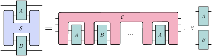
Figure B1: General simulation of the quantum switch. A higher-order transformation $\mathcal{C}$, which can be a quantum comb or a QC-CC, that acts on part of several copies of input bipartite quantum channels $A$ and $B$ is a simulation of the quantum switch $\mathcal{S}$ if it reproduces the action of the quantum switch for all arbitrary pairs of bipartite channels $A$ and $B$.

The first simulation scenario discussed in the main text is the one where the quantum switch $\mathcal{S}$ acts on the “entire” quantum channels $A$ and $B$, as represented in Fig. 2, in the main text. Formally, this is the case where the quantum switch $\mathcal{S}$ acts on a pair of single-party (single input system, single output system) channels $A:\mathcal{L}(\mathcal{H}^{A_{I}})\to\mathcal{L}(\mathcal{H}^{A_{O}})$ and $B:\mathcal{L}(\mathcal{H}^{B_{I}})\to\mathcal{L}(\mathcal{H}^{B_{O}})$, and outputs another channel $\mathcal{S}(A,B):\mathcal{L}(\mathcal{H}^{c_{I}}\otimes\mathcal{H}^{t_{I}})\to\mathcal{L}(\mathcal{H}^{c_{O}}\otimes\mathcal{H}^{t_{O}})$. However, quantum theory also allows one to apply the quantum switch on parts of bipartite (two input systems, two output systems) channels $A:\mathcal{L}(\mathcal{H}^{A_{I}}\otimes\mathcal{H}^{A^{\prime}_{I}})\to\mathcal{L}(\mathcal{H}^{A_{O}}\otimes\mathcal{H}^{A^{\prime}_{O}})$ and $B:\mathcal{L}(\mathcal{H}^{B_{I}}\otimes\mathcal{H}^{B^{\prime}_{I}})\to\mathcal{L}(\mathcal{H}^{B_{O}}\otimes\mathcal{H}^{B^{\prime}_{O}})$, where the dimension of the primed spaces is arbitrary. This results in the quantum channel $\mathcal{S}\otimes\mathcal{I}(A,B):\mathcal{L}(\mathcal{H}^{A^{\prime}_{I}}\otimes\mathcal{H}^{c_{I}}\otimes\mathcal{H}^{t_{I}}\otimes\mathcal{H}^{B^{\prime}_{I}})\to\mathcal{L}(\mathcal{H}^{A^{\prime}_{O}}\otimes\mathcal{H}^{c_{O}}\otimes\mathcal{H}^{t_{O}}\otimes\mathcal{H}^{B^{\prime}_{O}})$, where $\mathcal{I}$ is the identity higher-order transformation. Since the dimension of the primed spaces is arbitrary, all multi-partite channels can be described in this context as bipartite channels, which are the most general kinds of deterministic transformations between quantum states one should consider. This case is illustrated in Fig. 3 of the main text.

As mentioned in the main text, the impossibility of simulating the action of the quantum switch on all single-party quantum channels, for some number of calls $k_{A}$ and $k_{B}$, implies the impossibility of simulating the action of the quantum switch on all bipartite channels with the same number of calls. Hence, when focusing on no-go simulation proofs, we can restrict ourselves to considering only single-party channels. However, conversely, should a simulation of the action of the quantum switch on all single-party channels exist for some number of calls $k_{A}$ and $k_{B}$, this does not necessarily imply that a simulation would also exists for the action of the quantum switch on all bipartite channels.

For this reason, in order to have a fully general simulation of the quantum switch, one must consider the case where the quantum switch acts on only part of a bipartite channel, as illustrated in Fig. B1. That is, a full simulation of the quantum switch is only obtained when, for every pair of bipartite channels $A:\mathcal{L}(\mathcal{H}^{A_{I}}\otimes\mathcal{H}^{A^{\prime}_{I}})\to\mathcal{L}(\mathcal{H}^{A_{O}}\otimes\mathcal{H}^{A^{\prime}_{O}})$ and $B:\mathcal{L}(\mathcal{H}^{B_{I}}\otimes\mathcal{H}^{B^{\prime}_{I}})\to\mathcal{L}(\mathcal{H}^{B_{O}}\otimes\mathcal{H}^{B^{\prime}_{O}})$, there exists $k_{A},k_{B}\in\mathbb{N}$ such that,

$$\mathcal{C}(A^{\otimes k_{A}},B^{\otimes k_{B}})=\mathcal{S}\otimes\mathcal{I}(A,B)$$ (54)

where $\mathcal{C}$ is a quantum comb, or a QC-CC. This most general simulation scenario is depicted in Fig. B1.

In the next section, we show how a simulation of the action of the quantum switch on all pairs of bipartite channels indeed covers all possible quantum operations the quantum switch could take as input, including the probabilistic ones, such as quantum instruments.

B.2 The action of the quantum switch on quantum instruments

Higher-order transformations like the quantum switch can also be applied to quantum instruments, which describe the most general probabilistic transformation between quantum states.

Quantum instruments are transformations that map a quantum state to another quantum state with a certain probability, also outputting a classical outcome. Physically, this describes, for instance, a measurement process where both an outcome and a post-measurement state are produced. They can be described by a collection of CP maps $\{I_{a}\}_{a}$ which add to a CPTP map, i.e., such that $\sum_{a}I_{a}$ is CPTP. A quantum instrument takes a quantum state $\rho$ as input, and outputs a classical outcome $a$, together with the quantum state $\rho_{a}\coloneqq I_{a}[\rho]/\tr(I_{a}[\rho])$, with probability $p_{a}\coloneqq\tr(I_{a}[\rho])$. Quantum instruments can be equivalently represented by deterministic quantum channels, which instead of yielding a classical outcome, prepare an additional pure quantum state $\ket{a}$ as output that encodes the value of the instrument’s classical outcome $a$ in a perfectly discriminable manner [42, 43, 44]. In other words, a quantum instrument with $N\in\mathbb{N}$ outcomes $\{I_{a}\}_{a=1}^{N}$ with $I_{a}:\mathcal{L}(\mathcal{H}^{I})\to\mathcal{L}(\mathcal{H}^{O})$ is equivalent to a quantum channel $A:\mathcal{L}(\mathcal{H}^{I})\to\mathcal{L}(\mathcal{H}^{O}\otimes\mathbb{C}^{N})$ given by

$$A[\,\rho\,]\coloneqq\sum_{a=1}^{N}I_{a}[\,\rho\,]\otimes\outerproduct{a}{a},$$ (55)

and illustrated in Fig. B2$(b)$. By representing a quantum instrument as a particular case of a bipartite quantum channel, namely one with a single input system and two output systems, it is straightforward to see that the action of the quantum switch on a pair of instruments $\{I^{A}_{a}\}_{a}$ and $\{I^{B}_{b}\}_{b}$ constitutes a special case of its action on arbitrary bipartite channels $A$ and $B$. Hence, a simulation of the quantum switch for all bipartite channels can be used for a simulation of the quantum switch for all instruments.

Lastly, one might also consider the scenario where the quantum switch acts on parts of bipartite instruments. Notice, however, that from the channel representation of instruments, it is clear that this scenario is included in that of arbitrary bipartite channels discussed in the previous section.

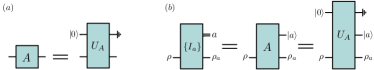
Figure B2: General quantum channels and quantum instruments. $(a)$ Quantum circuit representation of the Stinespring dilation $U_{A}$ of the general quantum channel $A$ presented in Eq. (56). $(b)$ Quantum circuit representation of a quantum instrument $\{I_{a}\}_{a}$ by a quantum channel $A[\rho]\coloneqq\sum_{a}I_{a}[\rho]\otimes\outerproduct{a}{a}$, which is then represented by its Stinespring dilation $U_{A}$.

B.3 The relationship with Stinespring dilation of quantum channels

Figure B3: The action of the quantum switch. Depiction of the action of the quantum switch on $(a)$ general single-party quantum channels; $(b)$ general single-party quantum instruments; $(c)$ part of general bipartite quantum channels, and; $(d)$ part of general bipartite quantum instruments; as a function of the action of the quantum switch on the Stinespring dilation of the input channels.

The Stinespring dilation theorem [24] states that the action of every general quantum channel, i.e, CPTP map, $A:\mathcal{L}(\mathcal{H}^{I})\to\mathcal{L}(\mathcal{H}^{O})$ can be written as

$$A[\,\rho\,]=\tr_{\text{aux}_{O}}\Big{(}U_{A}[\,\rho^{I}\otimes\outerproduct{0}{0}\,]\Big{)},$$ (56)

for some unitary channel $U_{A}:\mathcal{L}(\mathcal{H}^{I}\otimes\mathcal{H}^{\text{aux}_{I}})\to\mathcal{L}(\mathcal{H}^{O}\otimes\mathcal{H}^{\text{aux}_{O}})$ that acts jointly on the input system and an auxiliary system (of sufficiently large dimension), which can be initialised to the state $\ket{0}$ without loss of generality. We emphasise that the discarding of the output auxiliary system is necessary for the equivalence between non-unitary channels and their unitary channel dilation. This equivalence between arbitrary quantum channels and their unitary channel dilation is depicted in Fig. B2$(a)$. Additionally, note that the Stinespring dilation can be combined with the channel representation of a quantum instrument presented in Eq. (55), so that all instruments can also be viewed as a unitary channel that makes use of an auxiliary system which is later discarded, as depicted in Fig. B2$(b)$.

Exploiting the Stinespring dilation of general quantum instruments and general quantum channels into bipartite unitary channels that discard their auxiliary system, one can express the action—and consequently the simulation—of the quantum switch solely in terms of unitary channels. However, in order to do so, it is necessary to keep track of exactly which systems are acted upon, preserved, and discarded. In Fig. B3, we show precisely how the action of the quantum switch on the different kinds of inputs discussed so far can be expressed in terms of its action on unitary channels.

In Fig. B3$(a)$, we depict the action of the quantum switch on general single-party channels. In Fig. B3$(b)$, we represent the action of the quantum switch on single-party quantum instruments. In Fig. B3$(c)$, we show the action of the switch in its most general case: when it acts on only part of bipartite general channels. Finally, in Fig. B3$(d)$, the action of the switch on part of bipartite instruments is pictured. Trivially, the case in Fig. B3$(a)$ is a particular case of Fig. B3$(c)$. Notice, moreover, how both the cases of Fig. B3$(b)$ and $(d)$, concerning quantum instruments, are also particular cases of Fig. B3$(c)$. In the latter case in particular, this is because the dimension of the primed spaces of the input bipartite channels—the ones that the switch does not act upon—are arbitrary, and hence, the quantum outputs $\ket{a}$ and $\ket{b}$ of the instruments can be absorbed into the other output system of the unitary channels that is not acted upon by the quantum switch.

B.4 Theorem 1: A simulation for bipartite unitary channels $U_{A}$ and bipartite general channels $B$

In this section we prove Theorem 1 from the main text and discuss how this particular-case simulation compares to more general simulation scenarios. We start by restating Theorem 1:

Theorem 1.

The action of the quantum switch on part of bipartite quantum channels can be deterministically simulated by a quantum circuit that has access to an extra call to one the input channels, as long as that channel is restricted to being unitary.

In other words, if $A$ is a bipartite unitary channel and $B$ is a bipartite general channel, there exists a quantum circuit described by a higher-order transformation $\mathcal{C}$ that satisfies Eq. (8) for $k_{A}=2$ and $k_{B}=1$.

The proof is based on the explicit construction of the following quantum circuit, presented as Eq. (9) in the main text and repeated here for convenience:

$$\quantikz[columnsep=3.8mm]\lstick{{\hbox{c_I}}}&\ctrl{3}\ctrl{4}\ctrl{3}\ctrl{4}\ctrl[open]{3}\ctrl[open]{4}\ctrl[open]{3}\ctrl[open]{4}\rstick{{\hbox{c_O}}}\\ \lstick{{\hbox{{\text{aux}_1}_I}}}\targX{}\targX{}\targX{}\targX{}\rstick{{\hbox{{\text{aux}_1}_O}}}\\ \lstick{{\hbox{{\text{aux}_2}_I}}}\targX{}\targX{}\targX{}\targX{}\rstick{{\hbox{{\text{aux}_2}_O}}}\\ \lstick{{\hbox{A'_I}}}\targX{}\gate[2,style={fill=JessicaColour!30},labelstyle=black]{A}\targX{}\targX{}\gate[2,style={fill=JessicaColour!30},labelstyle=black]{A}\targX{}\rstick{{\hbox{A'_O}}}\\ \lstick{{\hbox{t_I}}}\targX{}\targX{}\gate[2,style={fill=JessicaColour!30},labelstyle=black]{B}\targX{}\targX{}\rstick{{\hbox{t_O}}}\\ \lstick{{\hbox{B'_I}}}\rstick{{\hbox{B'_O}}}$$ (57)

Proof.

Let $A:\mathcal{L}(\mathcal{H}^{A_{I}}\otimes\mathcal{H}^{A^{\prime}_{I}})\to\mathcal{L}(\mathcal{H}^{A_{O}}\otimes\mathcal{H}^{A^{\prime}_{O}})$ be a bipartite channel with Kraus operators $\{A_{i}\}$ where $A_{i}:\mathcal{H}^{A_{I}}\otimes\mathcal{H}^{A^{\prime}_{I}}\to\mathcal{H}^{A_{O}}\otimes\mathcal{H}^{A^{\prime}_{O}}$. Similarly, let $B:\mathcal{L}(\mathcal{H}^{B_{I}}\otimes\mathcal{H}^{B^{\prime}_{I}})\to\mathcal{L}(\mathcal{H}^{B_{O}}\otimes\mathcal{H}^{B^{\prime}_{O}})$ be a bipartite channel with Kraus operators $\{B_{i}\}$ where $B_{j}:\mathcal{H}^{B_{I}}\otimes\mathcal{H}^{B^{\prime}_{I}}\to\mathcal{H}^{B_{O}}\otimes\mathcal{H}^{B^{\prime}_{O}}$. The action of the quantum switch $\mathcal{S}$ on part of these channels results in the quantum channel $\mathcal{S}\otimes\mathcal{I}(A,B):\mathcal{L}(\mathcal{H}^{c_{I}}\otimes\mathcal{H}^{t_{I}}\otimes\mathcal{H}^{A^{\prime}_{I}}\otimes\mathcal{H}^{B^{\prime}_{I}})\to\mathcal{L}(\mathcal{H}^{c_{O}}\otimes\mathcal{H}^{t_{O}}\otimes\mathcal{H}^{A^{\prime}_{O}}\otimes\mathcal{H}^{B^{\prime}_{O}})$, whose definition is implied by Eqs. (1)-(2) and linearity. It is given by

$$\mathcal{S}\otimes\mathcal{I}(A,B)[\,\sigma_{c}\otimes\rho_{t}\otimes\omega_{A^{\prime}B^{\prime}}\,]=\sum_{i,j}S_{ij}(\sigma_{c}\otimes\rho_{t}\otimes\omega_{A^{\prime}B^{\prime}})S_{ij}^{\dagger},$$ (58)

where $\omega_{A^{\prime}B^{\prime}}\in\mathcal{L}(\mathcal{H}^{A^{\prime}_{I}}\otimes\mathcal{H}^{B^{\prime}_{I}})$ is an arbitrary state of the quantum system in the primed spaces of Alice and Bob, which are not acted upon by the quantum switch. Before explicitly writing the $S_{ij}$, it is convenient to decompose the Kraus operators $A_{i}$ and $B_{i}$ into linear combinations of operators that factorise between the primed and nonprimed spaces, which can always be done without loss of generality. It follows from linearity that one can always write

$$A_{i}=\sum_{a}\alpha_{a|i}\,A(a)\otimes A^{\prime}(a)$$ (59)

for some $\alpha_{a|i}\in\mathbb{C}$, $A(a):\mathcal{H}^{A_{I}}\to\mathcal{H}^{A_{O}}$, and $A^{\prime}(a):\mathcal{H}^{A^{\prime}_{I}}\to\mathcal{H}^{A^{\prime}_{O}}$. Similarly, one can write

$$B_{j}=\sum_{b}\beta_{b|j}\,B(b)\otimes B^{\prime}(b)$$ (60)

for some $\beta_{b|j}\in\mathbb{C}$, $B(b):\mathcal{H}^{B_{I}}\to\mathcal{H}^{B_{O}}$, and $B^{\prime}(b):\mathcal{H}^{B^{\prime}_{I}}\to\mathcal{H}^{B^{\prime}_{O}}$. Then, the Kraus operators $\{S_{ij}\}$ in Eq. (58) take the form

$$S_{ij}=\outerproduct{0}{0}\otimes\sum_{ab}\alpha_{a|i}\beta_{b|j}\,B(b)A(a)\otimes A^{\prime}(a)\otimes B^{\prime}(b)+\outerproduct{1}{1}\otimes\sum_{ab}\alpha_{a|i}\beta_{b|j}\,A(a)B(b)\otimes A^{\prime}(a)\otimes B^{\prime}(b),$$ (61)

where the order of the spaces from left to right in each term is control, target, and Alice and Bob’s primed systems.

The transformation of the quantum circuit in Eq. (9) that uses two calls of the quantum channel $A$ and a single call of the quantum channel $B$ in the order ABA results in a quantum channel $\mathcal{C}(A^{\otimes 2},B)$ which has Kraus operators

$$C_{ijk}=\outerproduct{0}{0}\otimes A_{k}\otimes\sum_{ab}\alpha_{a|i}\beta_{b|j}\,A^{\prime}(a)\otimes B(b)A(a)\otimes B^{\prime}(b)+\outerproduct{1}{1}\otimes A_{i}\otimes\sum_{ab}\alpha_{a|k}\beta_{b|j}A^{\prime}(a)\otimes A(a)B(b)\otimes B^{\prime}(b),$$ (62)

where the order of the spaces from left to right in each term coincides with the order of the wires from top to bottom in the quantum circuit in Eq. (9) (i.e., control, first auxiliary, second auxiliary, Alice’s primed, target, and Bob’s primed systems).

Whenever the bipartite channel $A=U_{A}$ is unitary, it has a single Kraus operator, i.e., $A[\rho]=A_{0}\rho A_{0}^{\dagger}$. Hence, following Eq. (61), in this case the quantum channel resulting from action of the quantum switch $\mathcal{S}\otimes\mathcal{I}(U_{A},B)$ has Kraus operators

$$S_{j}=\outerproduct{0}{0}\otimes\sum_{ab}\alpha_{a|0}\beta_{b|j}\,B(b)A(a)\otimes A^{\prime}(a)\otimes B^{\prime}(b)+\outerproduct{1}{1}\otimes\sum_{ab}\alpha_{a|0}\beta_{b|j}\,A(a)B(b)\otimes A^{\prime}(a)\otimes B^{\prime}(b).$$ (63)

Also in this case, following Eq. (62), the quantum channel resulting from action of the quantum circuit in Eq. (9) is described by the Kraus operators

$$C_{j} =\outerproduct{0}{0}\otimes A_{0}\otimes\sum_{ab}\alpha_{a|0}\beta_{b|j}\,A^{\prime}(a)\otimes B(b)A(a)\otimes B^{\prime}(b)+\outerproduct{1}{1}\otimes A_{0}\otimes\sum_{ab}\alpha_{a|0}\beta_{b|j}A^{\prime}(a)\otimes A(a)B(b)\otimes B^{\prime}(b)$$ (64)

$$=\left(\outerproduct{0}{0}\otimes\sum_{ab}\alpha_{a|0}\beta_{b|j}\,B(b)A(a)\otimes A^{\prime}(a)\otimes B^{\prime}(b)+\outerproduct{1}{1}\otimes\sum_{ab}\alpha_{a|0}\beta_{b|j}A(a)B(b)\otimes A^{\prime}(a)\otimes B^{\prime}(b)\right)\otimes A_{0}.$$ (65)

where, in the last line, we reordered the spaces from control, first auxiliary, second auxiliary, Alice’s primed, target, and Bob’s primed systems to control, target, and Alice and Bob’s primed, first auxiliary, and second auxiliary systems.

Note that the term in parenthesis is equal to that of Eq. (63). Hence, the action of the quantum switch on part of a bipartite unitary channel $A=U_{A}$ and a bipartite general channel $B$ is equivalent to the action of the quantum circuit in Eq. (9) that uses two calls of bipartite unitary channel $A=U_{A}$ and a single call of bipartite general channel $B$ in the order ABA. Moreover, note that one call of $A=U_{A}$ in the quantum circuit in Eq. (9) is recovered, since $A_{0}$ factorizes in Eq. (64). This phenomenon is referred to as a catalytic higher-order transformation in the literature [45], since the extra use of $A=U_{A}$ is recovered after the completion of the process. ∎

We now contrast the different scenarios of the action of the quantum switch presented in Apps. B.1–B.3 with the particular-case simulation of Theorem 1.

Let us begin with the circuit from Ref. [6], reproduced in Eq. (6), and depicted here as the quantum comb in Fig. B4$(a)$. This circuit simulates the action of the quantum switch on unitary channels by making use of one extra call to one of the input channels. Although every general quantum channel can be dilated into a unitary channel acting on a larger space, the simulation of the quantum switch on unitary channels in the case depicted in Fig. B4$(a)$ is not the most general case, because here the entire unitary channel is “plugged into” the open slots of the quantum switch and of the quantum comb that performs its simulation.

The simulation presented in Ref. [6], here in Fig. B4$(a)$, is a particular case of the simulation scenario we proved possible via the explicit construction of the quantum circuit in Eq. (9). Our generalization addresses the case where the quantum switch acts on only part of a unitary channel and part of a general quantum channel, with the simulation also requiring only one extra copy of the input unitary channel. We depict this scenario and our quantum circuit simulation as a quantum comb in Fig. B4$(b)$. Although more general than the previous result from Ref. [6], this simulation result still does not hold in the most general case, depicted in Fig. B1$(c)$, because the input quantum channel $U_{A}$ is required to be a unitary channel.

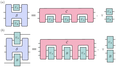
Figure B4: Quantum comb representation of possible quantum switch simulations. $(a)$ Representation of the simulation of the action of the quantum switch on single-party unitary channels as a quantum comb, presented in Ref. [6] and shown in Eq. (6) as a quantum circuit. $(b)$ Representation of the simulation of the action of the quantum switch on part of a bipartite unitary channel and part of a bipartite general quantum channel by a quantum comb, which we have shown to be possible by explicitly constructing the quantum circuit in Eq. (9).

The quantum switch simulation presented in Fig. B4$(b)$ is also useful to illustrate the crucial aspect of the partial trace involved in the Stinespring dilation. Notice that this simulation covers the scenario where $B$ is an arbitrary bipartite channel, and $U_{A}$ is an arbitrary bipartite unitary channel. Naïvely, one could expect that—since our simulation covers all bipartite unitary channels $U_{A}$—due to the Stinespring dilation theorem, this simulation would also apply to the case where $A$ is a single-party arbitrary quantum channel, as in Fig. B3$(a)$. However, this line of argumentation is false, as it is not possible to simulate the quantum switch for a pair of single-party arbitrary quantum channels, as proven in the main text. The logical gap in the argument is a misuse of the Stinespring dilation theorem, which requires the auxiliary system to be discarded, whereas in the simulation presented in Fig. B4$(b)$, there is no partial trace after the unitary operation $U_{A}$. When the auxiliary system of the Stinespring dilation is not discarded, the corresponding operation is not equivalent to the quantum channel in question. From this circuit simulation perspective, keeping track of the auxiliary systems may be viewed as a “loophole”, since the auxiliary system may carry additional information that is not provided by the channel $A$. To see this intuitively, consider a quantum channel $A$ with a Kraus decomposition given by $A(\rho)=\sum_{i}K_{i}\rho K_{i}^{\dagger}$ and which is dilated by the isometry $V=\sum_{i}K_{i}\otimes\ket{i}$, where $\ket{i}$ is a quantum state on the auxiliary system. The quantum state $\ket{i}$ may be viewed as a flag that indicates which Kraus operator was applied to $\rho$. If the flag state is not discarded, one could use this information to correlate Kraus elements between a first and a second call of the channel $A$, which cannot be done when the auxiliary system is traced out.

Appendix C Possible restricted simulations for qubit channels

Using numerical methods, we have found three particular cases where a restricted simulation of the quantum switch acting on qubit channels is possible, exactly and deterministically, using a quantum comb. These are the cases of:

• Four identical calls to general qubit channels, called the order AAAA.

• Two calls to unitary qubit channels $A$ and two calls to unitary qubit channels $B$, in the order AABB.

• Three calls to unitary qubit channels $A$ and one call to unitary qubit channels $B$, in the order BAAA.

All of these results were obtained by numerically evaluating the equivalent of the primal SDP (16) in the case where the input states are fixed and the output target system is discarded, and finding that $p=1$ up to a high numerical precision.

Effectively, this scenario amounts to an SDP that is analogous to SDP (16) but with the first constraint written as

$$C_{s}*\Big{[}{(J^{A}_{i})}^{\otimes k_{A}}\otimes{(J^{B}_{j})}^{\otimes k_{B}}\Big{]}=p\,\tr_{t_{O}}(S_{+0})*(J^{A}_{i}\otimes J^{B}_{j})\ \ \ \forall\,i,j,$$ (66)

where $S_{+0}$ is defined as in Eq. (25). In this case, we have that $C_{s},C\in\mathcal{L}(\mathcal{H}^{A_{I}}\otimes\mathcal{H}^{A_{O}}\otimes\mathcal{H}^{B_{I}}\otimes\mathcal{H}^{B_{O}}\otimes\mathcal{H}^{c_{O}})$ and $d_{c_{I}}=d_{t_{I}}=1$.

In the case of $4$ identical copies of general qubit channels, the input channels were given as a basis constructed in the form of Eq. (22). The dimension of the space spanned by $k=4$ identical copies of a general qubit channel is $d_{\mathcal{V}}=1820$, a value that can be obtained from the expression presented in Sec. IV of the main text.

In the case of $k$ identical copies of qubit unitary channels, a basis can be constructed numerically by randomly sampling a set of qubit unitaries according to the Haar measure, guaranteeing that they are linearly independent. It is only necessary to know the dimension of this subspace beforehand to determine how many unitaries must be sampled. The dimension of the linear space spanned by $k$ copies of $d$-dimension unitary channels is the quantity $D(d,r,s)$ of Ref. [46] for the case $r=s=k$. For $d=2$, the dimension of the subspace spanned by $k$ identical copies of a unitary channel is given by $d_{\mathcal{U}}=D(d=2,k,k)=\binom{2k+3}{3}$, which implies $d_{\mathcal{U}}=10$ for $k=1$, $d_{\mathcal{U}}=35$ for $k=2$, and $d_{\mathcal{U}}=84$ for $k=3$.

By numerically evaluating the appropriate SDP, we obtain that the maximum probability of success is $p=1$ with very high precision in all aforementioned cases. The numerical precision was evaluated in the following way: In all three cases, all inequality constrains are strictly satisfied; as for the equality constraints, they are satisfied up to an error of at most $10^{-9}$ in the operators norm for the case of identical general qubit channels AAAA, and at most $10^{-7}$ in the cases of qubit unitary channels AABB and BAAA.

We also found that the maximum probability of success remains $p=1$, with the same precision, in all three cases when the second and third slots of the quantum comb $\mathcal{C}$ are parallelized, as depicted in Fig. C1.

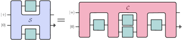
Figure C1: Semi-parallelized strategy for restricted qubit simulations. The quantum switch acting on qubit channels can be deterministically simulated by a $4$-slot quantum comb that has its second and third slots parallelized in a restricted scenario where the input control and target systems are fixed and the output target system is discarded in three different cases: for identical general quantum channels, i.e. when $A=B$, called order AAAA, and for unitary channels in the orders AABB and BAAA.

Impossible partly restricted simulation. As mentioned in the main text, we also found that when the output target system is not discarded—i.e., the partly restricted simulation scenario—then a deterministic simulation is no longer possible in all 3 aforementioned cases.

More concretely, this is the scenario where the first constraint in SDP (16) is written as

$$C_{s}*\Big{[}{(J^{A}_{i})}^{\otimes k_{A}}\otimes{(J^{B}_{j})}^{\otimes k_{B}}\Big{]}=p\,S_{+0}*(J^{A}_{i}\otimes J^{B}_{j})\ \ \ \forall\,i,j,$$ (67)

where $S_{+0}$ is defined as in Eq. (25), $C_{s},C\in\mathcal{L}(\mathcal{H}^{A_{I}}\otimes\mathcal{H}^{A_{O}}\otimes\mathcal{H}^{B_{I}}\otimes\mathcal{H}^{B_{O}}\otimes\mathcal{H}^{t_{O}}\otimes\mathcal{H}^{c_{O}})$, and $d_{c_{I}}=d_{t_{I}}=1$.

Evaluating the above SDP, for the partly restricted scenario, we found that $p<1$ in the AAAA case of identical general qubit channels, the AABB case of qubit unitary channels, as well as the BAAA case of qubit unitary channels. Due to limitations in computational power, the partly restricted simulation SDP was evaluated in all three cases with an input that corresponds to a subset of the basis that was given as input to the restricted simulation SDP. Therefore, the solutions for the maximal probability of success correspond to upper bounds, and are given by

order = AAAA (qubit, general),. $$p\leq 0.942$$ (68)

$$\text{order = AABB (qubit, unitary)},\ \ \ p\leq 0.822$$ (69)

$$\text{order = BAAA (qubit, unitary)},\ \ \ p\leq 0.667.$$ (70)

The difference between the two simulation scenarios discussed in this section is whether or not the output target state is discarded. Here we can see that this distinction in the requirements of the simulation is sufficient to transform cases where a deterministic simulation is possible (with a discarded output target system) into cases where a deterministic simulation is no longer possible (without discarding the output target system).

Appendix D No-go results for unitary channels

As previously discussed, the simulation of the action of the quantum switch on unitary channels is possible when an extra call of one of the input channels is available. This was first shown by Ref. [6] for the action of the quantum switch on entire single-party unitary channels, and here we have shown this result to extend to a more general scenario where the quantum switch acts only on part of the input unitary channels (see Theorem 1 in Sec. B.4). These results hold in the general simulation scenario, where the input systems are not fixed and the output systems are not discarded, and hold as well for any dimension.

However, this result crucially depends not only on the number of extra calls available, but also on the order in which the quantum unitary channels are applied in the simulation. The cases where a simulation is possible for either single-party or for bipartite unitary channels with $(k_{A},k_{B})=(2,1)$ use the order ABA. If the order of the applied channels is instead either AAB or BAA, we find that a deterministic simulation is no longer possible, even in the restricted qubit scenario.

Moreover, the existence of a simulation for unitary channels in the order ABA implies that, when $(k_{A},k_{B})=(2,2)$, a simulation with the orders ABAB and ABBA also trivially exists. In App. C, we showed that a simulation using the order AABB also exists for unitary channels, albeit only in the restricted qubit case where the output target system is discarded. For the case where $(k_{A},k_{B})=(3,1)$, a simulation in the orders AABA and ABAA exists, following trivially from the result for ABA. We showed in App. C that a simulation for unitary channels in the order BAAA exists as well, but once again only in the restricted qubit case. The one case left to study then is a simulation of the quantum switch acting on unitary channels in the order AAAB. We show such a simulation is not possible.

Hence, our three no-go results for simulations of the quantum switch acting exclusively on unitary channels concern the cases of:

• Two calls of the unitary channels $A$ and one call of unitary channels $B$, in the order AAB.

• Two calls of the unitary channels $A$ and one call of unitary channels $B$, in the order BAA.

• Three calls of the unitary channels $A$ and one call of unitary channels $B$, in the order AAAB.

In order to show these results, we numerically evaluate the maximum probability of success of simulating the quantum switch when the input channels are unitary. We do so in the case where the input channels are acting on qubit systems, i.e., when $d=2$, and in the restricted simulation scenario where the input control and target systems are fixed, and the output target system is discarded [see Eq. (66)]. We remark once again that the impossibility of a deterministic simulation in the restricted, fixed-dimension case implies the impossibility of a deterministic simulation in general.

In this case, we do not construct an explicit basis analytically for the subspace spanned by $k$ identical copies of a qubit unitary channel, but instead, we randomly sample a set of $d_{\mathcal{U}}$ linearly independent qubit unitary channels $\{U_{i}^{\otimes k}\}_{i=1}^{d_{\mathcal{U}}}$ to form our basis. We repeat here that for the case where $k=1$, $d_{\mathcal{U}}=10$, for $k=2$, $d_{\mathcal{U}}=35$, and for $k=3$, and $d_{\mathcal{U}}=84$. This implies that in the $(k_{A},k_{B})=(2,1)$ case, one needs $35\cdot 10=350$ pairs of qubit unitary channels and for $(k_{A},k_{B})=(3,1)$, one needs $84\cdot 10=840$ pairs of qubit unitary channels as input for the SDPs (16) and (17). We numerically obtain the values of

$$\text{order = AAB\phantom{A} (qubit, unitary)},\ \ \ p\approx 0.600$$ (71)

$$\text{order = BAA\phantom{A} (qubit, unitary)},\ \ \ p\approx 0.851$$ (72)

$$\text{order = AAAB (qubit, unitary)},\ \ \ p\approx 0.708.$$ (73)

Appendix E Efficient certification that a matrix is positive semidefinite

A self-adjoint linear operator $A\in\mathcal{L}(\mathbb{C}^{d})$ is positive semidefinite if and only if there exists an operator $L\in\mathcal{L}(\mathbb{C}^{d})$ such that $A=LL^{\dagger}$. Moreover, the operator $L$ can be taken to be a lower triangular matrix, i.e., a matrix in which all entries above the main diagonal are zero. The decomposition of a positive semidefinite matrix as $A=LL^{\dagger}$ is referred to as the Cholesky decomposition, and finding such a decomposition can be done efficiently [37].

In the final step of the algorithm used for computer-assisted proofs presented in Sec. IV of the main text, one is required to certify that an operator $A$ is positive semidefinite. When $A$ is stored as a symbolic matrix, due to the way computers manipulate symbolic variables, if the matrix $A$ is not sparse enough, ensuring that $A\geq 0$ may be a prohibitively time-consuming task even when using the Cholesky decomposition. This was the case, for instance, when trying to ensure that the matrix $\overline{\mathbb{P}}(\Gamma^{\texttt{sym}})+\eta\mathbb{1}-\sum_{i,j}R_{ij}^{\texttt{OK}}\otimes({J^{A}_{i}}^{\otimes k_{A}}\otimes{J^{B}_{j}}^{\otimes k_{B}})^{T}$ in our computer-assisted proofs algorithm involving $k_{A}+k_{B}=4$-slot quantum combs. Below, we describe an algorithm that can be used to ensure that a symbolic matrix $A$ is positive semidefinite, which is considerably faster than performing Cholesky decomposition on a symbolic matrix $A$.

The algorithm we present below is based on three key ideas.

1. It is possible to rigorously certify that a matrix is positive definite using floating-point arithmetic quickly. One way to attain this goal is to use the methods presented in Ref. [47]. It shows how to efficiently certify that a matrix $A$ is positive definite using a rigorous algorithm that accounts for all possible computational and rounding errors and remains valid in the presence of underflow.

2. If a matrix $A$ is “close” to another matrix $A^{\prime}$, and $A^{\prime}$ is “far” from the set of non-positive semidefinite matrices, then $A$ has to be positive semidefinite.

3. If $A$ is matrix with symbolic entries, we can obtain a floating-point variable matrix $A^{\prime}$ that is guaranteed to be close to $A$. This can be done via arbitrary-precision arithmetic [48].

Algorithm to prove that a symbolic self-adjoint matrix $A$ is positive semidefinite:

1. Construct a self-adjoint matrix $A^{\prime}$ that is equal to $A$ up to $n$ decimal digits
   This step can be accomplished using arbitrary-precision arithmetic [48] with a precision of $n$ decimal digits. In this way, all matrix elements of $A^{\prime}-A$ are between $-10^{-n+1}$ and $10^{-n+1}$, ensuring that

   $$-J\cdot 10^{-n+1}\;\leq\;A^{\prime}-A\;\leq\;J\cdot 10^{-n+1},$$ (74)

   where $J\geq 0$ is a matrix in which all entries are the number one.

2. Prove that $A^{\prime}-J\geq 0$ using the algorithm presented in Ref. [47].
   Since $A^{\prime}-J\cdot 10^{-n+1}\leq A$ holds, if we ensure that $A^{\prime}-J\geq 0$, then by transitivity it follows that $A\geq 0$.

References

- Chiribella et al. [2008a] G. Chiribella, G. M. D’Ariano, and P. Perinotti, Quantum Circuit Architecture, Phys. Rev. Lett. 101, 060401 (2008a), arXiv:0712.1325 [quant-ph] .
- Chiribella et al. [2008b] G. Chiribella, G. M. D’Ariano, and P. Perinotti, Transforming quantum operations: Quantum supermaps, EPL 83, 30004 (2008b), arXiv:0804.0180 [quant-ph] .
- Chiribella et al. [2009] G. Chiribella, G. M. D’Ariano, and P. Perinotti, Theoretical framework for quantum networks, Phys. Rev. A 80, 022339 (2009), arXiv:0904.4483 .
- Bisio and Perinotti [2019] A. Bisio and P. Perinotti, Theoretical framework for higher-order quantum theory, Proc. R. Soc. A 475, 20180706 (2019), arXiv:1806.09554 [quant-ph] .
- Milz and Quintino [2024] S. Milz and M. T. Quintino, Characterising transformations between quantum objects, ‘completeness’ of quantum properties, and transformations without a fixed causal order, Quantum 8, 1415 (2024), arXiv:2305.01247 [quant-ph] .
- Chiribella et al. [2013] G. Chiribella, G. M. D’Ariano, P. Perinotti, and B. Valiron, Quantum computations without definite causal structure, Phys. Rev. A 88, 022318 (2013), arXiv:0912.0195 [quant-ph] .
- Oreshkov et al. [2012] O. Oreshkov, F. Costa, and Č. Brukner, Quantum correlations with no causal order, Nat. Commun. 3, 1092 (2012), arXiv:1105.4464 [quant-ph] .
- Araújo et al. [2015] M. Araújo, C. Branciard, F. Costa, A. Feix, C. Giarmatzi, and Č. Brukner, Witnessing causal nonseparability, New J. Phys. 17, 102001 (2015), arXiv:1506.03776 [quant-ph] .
- Chiribella [2012] G. Chiribella, Perfect discrimination of no-signalling channels via quantum superposition of causal structures, Phys. Rev. A 86, 040301 (2012), arXiv:1109.5154 [quant-ph] .
- Bavaresco et al. [2021] J. Bavaresco, M. Murao, and M. T. Quintino, Strict Hierarchy between Parallel, Sequential, and Indefinite-Causal-Order Strategies for Channel Discrimination, Phys. Rev. Lett. 127, 200504 (2021), arXiv:2011.08300 [quant-ph] .
- Bavaresco et al. [2022] J. Bavaresco, M. Murao, and M. T. Quintino, Unitary channel discrimination beyond group structures: Advantages of sequential and indefinite-causal-order strategies, J. Math. Phys. 63, 042203 (2022), arXiv:2105.13369 [quant-ph] .
- Zhao et al. [2020] X. Zhao, Y. Yang, and G. Chiribella, Quantum Metrology with Indefinite Causal Order, Phys. Rev. Lett. 124, 190503 (2020), arXiv:1912.02449 [quant-ph] .
- Liu et al. [2023] Q. Liu, Z. Hu, H. Yuan, and Y. Yang, Optimal strategies of quantum metrology with a strict hierarchy, Phys. Rev. Lett. 130, 070803 (2023), arXiv:2203.09758 [quant-ph] .
- Araújo et al. [2014] M. Araújo, F. Costa, and Č. Brukner, Computational Advantage from Quantum-Controlled Ordering of Gates, Phys. Rev. Lett. 113, 250402 (2014), arXiv:1401.8127 .
- Abbott et al. [2024] A. A. Abbott, M. Mhalla, and P. Pocreau, Quantum query complexity of boolean functions under indefinite causal order, Phys. Rev. Res. 6, L032020 (2024), arXiv:2307.10285 [quant-ph] .
- Quintino et al. [2019a] M. T. Quintino, Q. Dong, A. Shimbo, A. Soeda, and M. Murao, Reversing Unknown Quantum Transformations: Universal Quantum Circuit for Inverting General Unitary Operations, Phys. Rev. Lett. 123, 210502 (2019a), arXiv:1810.06944 [quant-ph] .
- Quintino et al. [2019b] M. T. Quintino, Q. Dong, A. Shimbo, A. Soeda, and M. Murao, Probabilistic exact universal quantum circuits for transforming unitary operations, Phys. Rev. A 100, 062339 (2019b), arXiv:1909.01366 [quant-ph] .
- Yoshida et al. [2023a] S. Yoshida, A. Soeda, and M. Murao, Universal construction of decoders from encoding black boxes, Quantum 7, 957 (2023a), arXiv:2110.00258 [quant-ph] .
- Yoshida et al. [2024] S. Yoshida, A. Soeda, and M. Murao, Universal adjointation of isometry operations using transformation of quantum supermaps (2024), arXiv:2401.10137 [quant-ph] .
- Poyatos et al. [1997] J. F. Poyatos, J. I. Cirac, and P. Zoller, Complete Characterization of a Quantum Process: The Two-Bit Quantum Gate, Phys. Rev. Lett. 78, 390 (1997), arXiv:quant-ph/9611013 .
- Chuang and Nielsen [1997] I. L. Chuang and M. A. Nielsen, Prescription for experimental determination of the dynamics of a quantum black box, J. Mod. Opt. 44, 2455 (1997).
- Milz et al. [2018] S. Milz, F. A. Pollock, T. P. Le, G. Chiribella, and K. Modi, Entanglement, non-Markovianity, and causal non-separability, New J. Phys. 20, 033033 (2018), arXiv:1711.04065 [quant-ph] .
- Rozema et al. [2024] L. A. Rozema, T. Strömberg, H. Cao, Y. Guo, B.-H. Liu, and P. Walther, Experimental aspects of indefinite causal order in quantum mechanics, Nature Reviews Physics 6, 483 (2024), arXiv:2405.00767 [quant-ph] .
- Watrous [2018] J. Watrous, The Theory of Quantum Information (Cambridge University Press, 2018).
- Wechs et al. [2021] J. Wechs, H. Dourdent, A. A. Abbott, and C. Branciard, Quantum Circuits with Classical Versus Quantum Control of Causal Order, PRX Quantum 2, 030335 (2021), arXiv:2101.08796 [quant-ph] .
- Ebler et al. [2018] D. Ebler, S. Salek, and G. Chiribella, Enhanced Communication with the Assistance of Indefinite Causal Order, Phys. Rev. Lett. 120, 120502 (2018), arXiv:1711.10165 [quant-ph] .
- Kristjánsson et al. [2024] H. Kristjánsson, T. Odake, S. Yoshida, P. Taranto, J. Bavaresco, M. T. Quintino, and M. Murao, Exponential separation in quantum query complexity of the quantum switch with respect to simulations with standard quantum circuits (2024), arXiv:24xx.xxxx [quant-ph] .
- Rubino et al. [2021] G. Rubino, L. A. Rozema, D. Ebler, H. Kristjánsson, S. Salek, P. A. Guérin, A. A. Abbott, C. Branciard, Č. Brukner, G. Chiribella, et al., Experimental quantum communication enhancement by superposing trajectories, Phys. Rev. Res. 3, 013093 (2021), arXiv:2007.05005 [quant-ph] .
- Cao et al. [2023] H. Cao, J. Bavaresco, N.-N. Wang, L. A. Rozema, C. Zhang, Y.-F. Huang, B.-H. Liu, C.-F. Li, G.-C. Guo, and P. Walther, Semi-device-independent certification of indefinite causal order in a photonic quantum switch, Optica 10, 561 (2023), arXiv:2202.05346 [quant-ph] .
- Antesberger et al. [2024] M. Antesberger, M. T. Quintino, P. Walther, and L. A. Rozema, Higher-order process matrix tomography of a passively-stable quantum switch, PRX Quantum 5, 010325 (2024), arXiv:2305.19386 [quant-ph] .
- Goswami et al. [2020] K. Goswami, Y. Cao, G. A. Paz-Silva, J. Romero, and A. G. White, Increasing communication capacity via superposition of order, Phys. Rev. Res. 2, 033292 (2020), arXiv:1807.07383 [quant-ph] .
- Guo et al. [2020] Y. Guo, X.-M. Hu, Z.-B. Hou, H. Cao, J.-M. Cui, B.-H. Liu, Y.-F. Huang, C.-F. Li, G.-C. Guo, and G. Chiribella, Experimental Transmission of Quantum Information Using a Superposition of Causal Orders, Phys. Rev. Lett. 124, 030502 (2020), arXiv:1811.07526 [quant-ph] .
- Chiribella and Kristjánsson [2019] G. Chiribella and H. Kristjánsson, Quantum Shannon theory with superpositions of trajectories, Proc. R. Soc. A 475, 20180903 (2019), arXiv:1812.05292 [quant-ph] .
- Kristjánsson et al. [2021] H. Kristjánsson, W. Mao, and G. Chiribella, Witnessing latent time correlations with a single quantum particle, Phys. Rev. Res. 3, 043147 (2021), arXiv:2004.06090 [quant-ph] .
- Skrzypczyk and Cavalcanti [2023] P. Skrzypczyk and D. Cavalcanti, Semidefinite Programming in Quantum Information Science (IOP Publishing, 2023).
- Chiribella and Ebler [2016] G. Chiribella and D. Ebler, Optimal quantum networks and one-shot entropies, New J. Phys. 18, 093053 (2016), arXiv:1606.02394 [quant-ph] .
- [37] https://en.wikipedia.org/wiki/cholesky_decomposition, accessed on 26/09/2024.
- [38] M. T. Quintino and J. Bavaresco, https://github.com/mtcq/switch_simulation.
- O’Donoghue et al. [2016] B. O’Donoghue, E. Chu, N. Parikh, and S. Boyd, Conic Optimization via Operator Splitting and Homogeneous Self-Dual Embedding, J. Optim. Theory Appl. 169, 1042 (2016), arXiv:1312.3039 [math.OC] .
- O’Donoghue et al. [2023] B. O’Donoghue, E. Chu, N. Parikh, and S. Boyd, SCS: Splitting conic solver, version 3.2.6, https://github.com/cvxgrp/scs (2023).
- MOSEK ApS [2024] MOSEK ApS, The MOSEK optimization toolbox for MATLAB manual. Version 10.1. (2024).
- Ozawa [1984] M. Ozawa, Quantum measuring processes of continuous observables, J. Math. Phys. 25, 79 (1984).
- Wilde [2017] M. M. Wilde, Quantum Information Theory, 2nd ed. (Cambridge University Press, 2017) arXiv:1106.1445 [quant-ph] .
- Buscemi et al. [2023] F. Buscemi, K. Kobayashi, S. Minagawa, P. Perinotti, and A. Tosini, Unifying different notions of quantum incompatibility into a strict hierarchy of resource theories of communication, Quantum 7, 1035 (2023), arXiv:2211.09226 [quant-ph] .
- Yoshida et al. [2023b] S. Yoshida, A. Soeda, and M. Murao, Reversing Unknown Qubit-Unitary Operation, Deterministically and Exactly, Phys. Rev. Lett. 131, 120602 (2023b), arXiv:2209.02907 [quant-ph] .
- Roy and Scott [2009] A. Roy and A. J. Scott, Unitary designs and codes, Des. Codes Cryptogr. 53, 13–31 (2009), arXiv:0809.3813 [math.CO] .
- Rump [2006] S. M. Rump, Verification of positive definiteness, BIT Numer. Math. 46, 433 (2006).
- [48] https://en.wikipedia.org/wiki/arbitrary-precision_arithmetic, accessed on 26/09/2024.