Soil organic carbon sequestration potential and policy optimization

Abstract

Land management could help mitigate climate change by sequestering atmospheric carbon dioxide as soil organic carbon (SOC). The impact of a given management change on the SOC content of a given volume of soil is generally unknown, but is likely moderated by features of the land that collectively determine its sequestration potential. To maximize sequestration, management interventions should be preferentially applied to fields with the highest sequestration potential and the lowest cost of application. We present a design-based statistical framework for estimating sequestration potential, average treatment effects, and optimal management policies from a randomized experiment with baseline covariate information. We review the myriad and nested sources of uncertainty that arise in this context and formalize the problem using potential outcomes. We show that a particular regression estimator—regressing field-level SOC on management indicators and their interactions with covariates—can help identify effective policies. The regression estimator also gives asymptotically valid inference on average treatment effects under the randomized design—without modeling assumptions—and can increase precision and power compared to the difference-in-means $T$-test. We conclude by discussing the saturation hypothesis in relation to sequestration potential, other study designs including observational studies of SOC, models for policy costs, nonparametric inference, and broader policy uncertainties.

1 Introduction

Global soils contain approximately double the amount of carbon stored in the atmosphere (Le Quéré et al., 2018), despite significant declines since the expansion of industrial agriculture (Sanderman et al., 2017). If some soil organic carbon (SOC) could be restored, it would reduce the amount of CO2 in the atmosphere. Because negative emissions are necessary to curtail the effects of climate change, governments and scientists have stepped up research into SOC sequestration as a “natural climate solution” (Bossio et al., 2020). This in turn has tilled enthusiasm in a stewardship philosophy and cluster of agricultural management techniques collectively called “regenerative agriculture.” Regenerative agriculture aims to improve ecosystem and soil health in a holistic sense, with SOC sequestration as a (potential) co-benefit (Lal, 2020). A large and growing body of empirical work aims to evaluate these claims, inquiring into the effects of land management changes (e.g., no-till agriculture, cover cropping, management-intensive grazing, etc) on SOC levels. Such research informs billions of dollars in policy investment (Stanford University, 2021; Minasny et al., 2017). To justify these investments policy makers must attribute SOC increases to management interventions and, ideally, tailor policies for maximum impact.

Unfortunately, several knowledge gaps currently jeopardize the effectiveness of policies aimed at SOC sequestration. In particular, the amount of SOC that could be sequestered in a given soil after a given intervention is unknown. This sequestration potential is critical to understand because it determines what a proposed policy can accomplish, including the amount of C sequestered, the rate of drawdown, and the longevity of the storage. Sequestration potential is an inherently causal concept, involving a comparison between the effects of two or more courses of action on the same soil.

To illustrate, suppose a hypothetical policy-maker is tasked with deciding whether to pay for a policy implementing no-till agriculture across all cropland in the US Corn Belt (the target population). Ideally, they would know the total amount of SOC in the top 1m of soil on each farm in (say) 10 years, both if that farm adopted no-till agriculture and if that farm were tilled annually. These quantities, only one of which can ever be observed on a given plot, are called potential outcomes. As a function of time, potential outcomes are called potential trajectories (Figure 1). If the policymaker knew all the potential trajectories within a population of farms, they could take nuanced actions to optimize sequestration given farm-specific timing, costs, and benefits associated with each intervention. This paper describes methods to estimate optimal policies (defined in terms of unknown potential outcomes) using empirical proxies of sequestration potential.

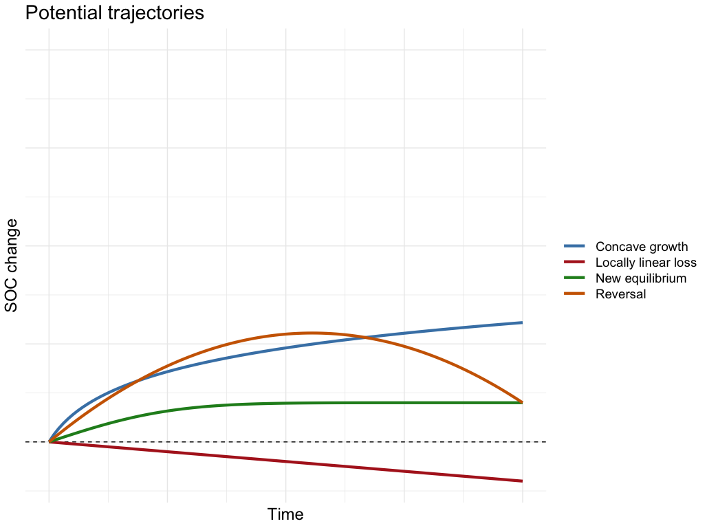
Figure 1: An illustration of four idealized population-level potential trajectories (colored lines) in terms of additional SOC sequestered (y-axis) over time (x-axis). From the point a decision is implemented, each course of action leads to a different trajectory of total SOC sequestered across the population. The trajectories are smoothed and do not reflect short-term variation like seasonality. A policy-maker with access to all potential trajectories and a target sequestration timeline could make optimal decisions under budgetary constraints. By definition, potential trajectories are equal at baseline (left most point on x-axis). The baseline SOC level is denoted by the dashed line. Under the green trajectory, SOC approaches a new equilibrium after the change has occurred, as theorized in Stewart et al. (2007) Under the blue and red trajectories, equilibrium is not achieved by the end of the time span plotted. The red trajectory displays a linear loss of SOC, as found, for example, in the study of Sanford et al. (2012). Under the orange trajectory there is a reversal, a major concern of policies aiming to sequester SOC as a negative emissions strategy (Smith, 2005; Thamo and Pannell, 2016). Researchers will often need to assume that trajectories are monotone, equilibrium is reached and maintained, and/or there are no future sequestration reversals when defining outcomes, designing studies, and interpreting results to make policy decisions.

1.1 Interventions

Management interventions can take many different forms, so a brief taxonomy is useful. Broadly, interventions may be policy changes or physical changes and they are not equivalent: paying a farmer to stop tilling their land is not the same as stopping tillage, since the farmer may not comply. Intervention as policy change is relevant to real-world policy decisions, while intervention as physical change is more directly relevant to scientists (who seek to understand mechanism) and to individual farmers (who are directly in control of their operation).

Interventions may be implemented at a single point in time (e.g., bolus of an input) or a pattern continuing over time (e.g., yearly application of inputs). Some interventions (e.g., land-use change or adoption of conservation tillage) involve a phase transition that may or may not continue over time. To avoid ambiguity, it is best to explicitly define the intervention as a pattern over time when designing and interpreting studies (e.g., to disambiguate whether “conservation tillage” entails merely a switch at baseline or indefinite maintenance of the practice). Hereafter, we assume that the intervention is fully defined at baseline either as a point-in-time or a pattern over time.

Interventions can be conceptualized as quantities, discrete categories, or both. Quantitative interventions include amendments like compost, manure, fertilizer, or biochar application, which are readily summarized in terms of the amount applied (in total, per hectare, and/or per unit time). Categorical interventions include converting tillage practices, adopting adaptive multi-paddock (AMP) grazing, and land-use change. A study that compares various intensities of compost and various intensities of chemical fertilizer contains both quantitatively and categorically different interventions.

Interventions are often framed in terms of their levels of C input, which may be more or less abstract. In particular, the level of C input can be known for some quantitative interventions (e.g. compost), but generally cannot for categorical interventions (e.g. adopting AMP grazing). Nevertheless, it is often useful to theorize about interventions simply in terms of their C input, especially when comparing responses across treatment types and treatment intensities (understood in terms of C input). Relating C input to SOC gain is an important dimension of sequestration potential.

1.2 Sequestration potential and saturation

The effectiveness of interventions is determined by the mechanisms that govern SOC sequestration. Interventions change SOC levels by changing the amount of C input to the soil and by changing the biological, chemical, and physical conditions that fix C. Broadly speaking, sequestration occurs when C input exceeds loss from decomposition, which varies as a function of environmental factors and soil properties. When C inputs and losses are balanced, SOC is at equilibrium (Chenu et al., 2019). After an external change, SOC tends toward a new equilibrium over time (Figure 1). Sequestration potential thus depends on both the nature of the management intervention (influencing the C input rate and potentially the decomposition rate) and on the capacity of a given soil volume to retain additional SOC under that intervention. Critically, the starting concentration of SOC in a given soil may influence the decomposition rate, and hence the soil’s capacity to store new C after an intervention. In the most extreme manifestation of this pattern, soils would have no additional capacity to store additional SOC under any intervention after the SOC level has reached a maximum amount: the SOC saturation hypothesis (Hassink, 1997). In its original form, this hypothesis states that soils have a finite capacity to store SOC because SOC is critically protected from decomposition by complexation with silt and clay sized minerals; once the available mineral surface area is exhausted, no additional C can be stored (Hassink, 1997). The precise dynamics depend on a complex interplay between the minerality and microbial biology of the soil, which can themselves change as a function of time and inputs. Empirical evidence for the SOC saturation hypothesis remains debated (Slessarev et al., 2023; Begill et al., 2023).

Regardless of the exact mechanism, C saturation is expected to result in diminishing storage of additional SOC as C inputs increase, with an eventual plateau once the soil is fully saturated (Stewart et al., 2007). Conversely, if saturation does not occur, increasing C inputs might yield a linear increase in SOC storage. Different soil types may exhibit behavior in response to different types of treatment and/or the intensity of quantitative treatment. For example, drier mineral soils could exhibit saturation while organic wetland soils could exhibit linear returns to inputs (Gorham, 1991). Alternatively, the reality for a given soil may be intermediate between these two extreme cases, with gains in SOC diminishing but not plateauing as C inputs increase. Four possibilities are presented in Figure 2.

However, not all interventions can be quantified in terms of C inputs, nor does total input sufficiently characterize the impact of any given intervention on SOC dynamics. In particular, additional complexity is necessary to theorize saturation when interventions are discrete (e.g., tillage vs no-till or conventional vs regenerative grazing) or when comparing quantitative C inputs applied in different forms (e.g., compost vs manure vs biochar). In canonical formulations of the saturation hypothesis, a discrete intervention may create a threshold—an effective stabilization capacity—below the absolute saturation limit by altering the decomposition rate of the soil (Stewart et al., 2007). For instance, conventional tillage and no-till strategies may produce different effective stabilization capacities, both of which lie below the saturation threshold. The actual saturation threshold is then defined by a counterfactual scenario in which C inputs are maximized and disturbance is minimized (as in a native or wild state).

If the saturation hypothesis is true, management interventions are expected to have less impact on fields near their saturation threshold. Thus, all else being equal, baseline SOC levels may moderate the effect of interventions on SOC sequestered, proxy sequestration potential, and predict treatment effects. Fractionating mineral soils into mineral associated organic carbon (MAOC) and particulate organic carbon (POC) could yield better empirical proxies to long-term sequestration potential: the MAOC pool is hypothesized to be both more stable and more susceptible to saturation than the POC pool (Cotrufo et al., 2019; Begill et al., 2023).

Proxies for sequestration potential—total baseline SOC, baseline MAOC, or other features—might play two key roles in policy decisions. First, they could improve estimates of average treatment effects, which correspond to the effect of a policy applied uniformly across a population and are often poorly constrained (Georgiou et al., 2022; Viscarra Rossel et al., 2024). Such estimates are critical to regional, national, and international C accounting and mitigation projections within larger portfolios of positive and negative emissions (e.g., International Energy Agency (2023)). However, real-world policy decisions involve more refined actions. For example, some plots may sequester more carbon when treated, while others respond better to control. Furthermore, resources are constrained in the real world, and usually only a limited number of plots in a population can be treated. Proxies of sequestration potential could help determine which plots to treat and how in order to maximize the overall impact of a budgeted policy.

1.3 Agents and Goals

There are countless actors—human and nonhuman—who stand to gain or lose from actions taken on any given plot of land, let alone across a population of $N$ plots. A reduction of this network has $N+1$ unique agents: a land manager for each plot $i$, and a policy-maker in charge of managing the population. We focus on the role of the policy-maker, and only consider the effects of interventions on SOC sequestration, although they will usually affect many other aspects that are externalities in our development. We return to this topic in our discussion.

More precisely, we consider the goal of maximizing SOC sequestration across a population when management decisions are controlled by an idealized, omnipotent policy-maker. Such a system may be unsustainable, inefficient, impractical, or unjust compared to alternatives that distribute power or influence over management decisions to prioritize local judgement and stewardship (Berry, 2004; Scott, 1999). Temporarily suspending these concerns, we will take the goal as given and focus on the practicalities of meeting it by statistical inference. The litany of uncertainties involved in gathering evidence to inform centralized decisions make the task difficult, even in idealized circumstances.

1.4 Outline

In the remainder of this paper, we address measurement challenges and present a strategy to optimize sequestration given empirical proxies for sequestration potential. Section 2 lays out the hierarchy of uncertainties inherent to quantifying the effects of interventions on SOC stock. We then formalize the overall policy objective of maximizing SOC sequestration across a population in Section 3. Section 4 provides a strategy for estimating sequestration potential and the optimal policy using empirical data. In Section 5 we present a simulation study based on data from a study of compost application on California rangelands, we compare the effectiveness of our proposed methods against various alternatives. Section 6 concludes with a discussion of additional uncertainties, limitations of our methods, policy implications, and directions for future research in this area.

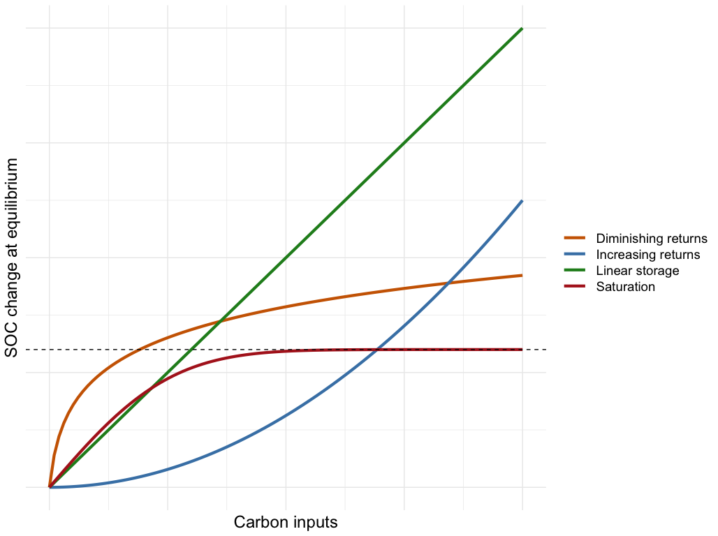
Figure 2: SOC at equilibrium ($y$-axis) as a function of C inputs from the intervention ($x$-axis) for various response possibilities (colors). C inputs may be thought of as a single pulse for a point treatment, or a total or average over time for a continuing treatment. The plot assumes all underlying potential trajectories reach equilibrium (see Figure 1). The red curve demonstrates complete saturation, wherein increasing inputs cannot increase equilibrium SOC above a certain point, the saturation threshold (dotted line) (Stewart et al., 2007). The orange curve represents partial saturation, wherein there are diminishing returns to inputs but returns do not encounter a threshold. This possibility could arise under partial saturation, whereby a soil can be partitioned into two pools, one of which saturates entirely while the other does not (Hassink, 1997; Stewart et al., 2007; Cotrufo et al., 2019) The green curve entails no saturation whatsoever: returns are linear at any level of input. Peat soils are an instance of linear storage, as anaerobic conditions prevent decomposition (Gorham, 1991). Note that when all inputs come from the intervention, this scenario implies perfect storage but no sequestration. Finally, the blue curve represents increasing returns to inputs, which could occur, for example, if a dead soil is progressively restored as inputs are increased. Increasing returns are implied, for example, by 17th century theories of fertilization advanced by early agricultural chemists including Robert Boyle and Benjamin Worlsey, who borrowed from the much older alchemical concept of multiplicatio (Niermeier-Dohoney, 2022). Boyle wrote “the seminal principle of nitre [i.e., KNO₃ or ‘saltpeter’], latent in the earth, does, by degrees, transform the neighbouring matter into a nitrous body” (Boyle, 1661).

2 Measuring the effects of management interventions

Sequestration studies aim to evaluate whether and how much a proposed treatment will increase SOC stock. They are subject to a hierarchy of uncertainties—at the core, plot, study, and population scale—all of which must be controlled and, when possible, quantified in uncertainty estimates like confidence intervals. Additional uncertainties arise when translating study interventions to policy interventions. We begin our exposition at the most granular of SOC uncertainties—the core-level—and zoom out from there.

2.1 Core-level uncertainties

To measure SOC stock, investigators take soil cores and measure them for SOC concentration (%SOC) and dry bulk density (BD) or equivalent soil mass (ESM; see next section). At the core level, uncertainties in %SOC arise from laboratory sample preparation protocols, human error, subsampling variability, and instrument error, which we collectively call assay variability. Assay variability can be addressed through careful laboratory work, including the use of precise instruments (e.g., elemental analyzers) and analytical replicates to control and estimate subsampling and instrument error. BD measurements are also subject to core-level uncertainties, including compression of soils during sampling, the presence of coarse fragments (e.g., gravel) in BD cores, and residual moisture. All of these factors need to be controlled through clear protocols, careful field work, and accounting. Finally, when MAOC is used to proxy saturation, the soil fractionation process requires a specific range of shaking or ultrasonic intensities to release the fine fraction without breaking up the coarse fraction and thereby contaminating the MAOC measurement with POC Amelung and Zech (1999); Six et al. (2024).

2.2 Plot-level uncertainties

Plot-level uncertainties are often more substantial than core-level (Stanley et al., 2023). The main source of plot-level uncertainty is the variability of %SOC and BD across space–spatial heterogeneity–which can be estimated by random sampling. When heterogeneity is high, no single core is representative of the total stock in a given plot. Larger samples are needed to detect and quantify realistic stock changes when spatial heterogeneity is high, and typical sample sizes may be far too small (Kravchenko and Robertson, 2011; Stanley et al., 2023). In some cases, stratification or balanced sampling can help to control spatial heterogeneity while keeping sample sizes and costs relatively low (de Gruijter et al., 2016; Potash et al., 2023). Compositing sampled cores before assay may also reduce costs or increase precision, but the potential benefits are sensitive to the costs and errors associated with sampling and assay; compositing also introduces more opportunities for user-error (Spertus, 2021; Stanley et al., 2023). BD change contributes uncertainty to stock change measurements depending on how sampling depth is determined. In particular, if samples are taken to a fixed depth, changes in BD (e.g., from soil compaction) can impact the measured SOC stock, even when the true SOC stock has not changed. The equivalent soil mass (ESM) procedure (Wendt and Hauser, 2013), attempts to navigate this issue, but changes the subject somewhat: stock change is expressed on a mass-mass basis, with BD measurements used only to determine the depth window over which the mass-mass average is taken. ESM also introduces a modeling uncertainty, as the cumulative soil mass to SOC mass relationship must be estimated using a cubic spline.

Other sources of plot-level uncertainty are often overlooked but may be substantial. One such source is the presence of large rocks (i.e. boulders) in plots (especially on rangelands) that affect the volume of actual SOC-bearing soil. When rocks are not taken into account, stock estimates may be biased upwards and estimates of change may be attenuated. Unfortunately, precise accounting for large rocks–those larger than a soil corer or bulk density ring–is difficult and is not done in most studies, but at the very least their presence should be noted. Another source of uncertainty in volumetric SOC measurement is negative correlation between %SOC and BD, which necessitates joint core-wise estimates of the two quantities across a plot. The common practice of estimating plot-level BD at a single pit using the ring method does not produce the data necessary to avoid this bias. Accurate, unbiased plot-level stock estimates require %SOC and BD to be measured on each core, volumetric concentrations to be computed at the core level, and the average of these concentrations to be taken as the average stock estimate (the estimate of the total being scaled according to the volume of soil).

2.3 Study-level uncertainties

Study-level uncertainties arise when conclusions are based on a study involving multiple plots. Usually, those conclusions answer an explicit or implicit causal question. A study without two or more known interventions cannot address causality. Hence, a study that only measures SOC on a group of plots at a point or multiple points in time is not suited to answer any causal question. Rather, the plots must be partitioned into two or more groups corresponding to different interventions and the outcome of interest (e.g. %SOC) compared between the groups. When the interventions are deliberately manipulated by the researcher the study is an experiment; when interventions are not manipulated by the researcher the study is an observational study. In this paper, our focus is on experiments—specifically randomized controlled trials (RCTs)—but we will briefly review uncertainties specific to observational studies as their shortcomings highlight the ideal role of experiments in causal inference.

Observational studies

Observational studies are subject to all of the uncertainties that arise in experiments (see the next section), plus additional issues inherent to drawing causal conclusions without manipulating the intervention. In particular, confounding occurs in observational studies when the receipt of treatment is influenced by baseline factors that are associated with the outcome. For example, if plots with lower baseline SOC are more likely to receive a compost amendment, simply comparing the observed averages of followup SOC between compost and no-compost plots will tend to provide a downward-biased estimate of the treatment effect because baseline SOC is positively associated with followup SOC. In that case, baseline SOC would be a confounder because it influences both the receipt of treatment and the outcome. When baseline SOC is measured, it is possible to adjust for its influence, and this extends to other possible confounders like weather, soil type, topography, land use etc. However, it is generally impossible to guarantee that all confounders were measured and properly accounted for, so conclusions are sensitive to assuming that they were. Ultimately, confounding is the rule, not the exception, in observational studies, and the rigor of conclusions drawn from them cannot be guaranteed.

As a further weakness, some observational studies do not even capture data over time (e.g., at baseline and followup), but record two groups of plots at a single time point. These so-called “space-for-time” studies are even more sensitive to bias since, without data on baseline SOC, a crucial confounder is missing.

Randomized controlled trials

RCTs are experiments wherein interventions are randomly assigned to plots following a known probability distribution—the design—possibly using additional control features such as blocking. Agricultural experiments are old. The development of their theory and practice played an important part in the modernization of scientific method during the 17th century (Niermeier-Dohoney, 2022). Enrolling multiple plots was established as a key feature of a successful agricultural experiment in the mid-18th century (Johnston, 1849), but the central role of randomization was not recognized until RA Fisher’s work at Rothamsted in the early 20th century (Fisher, 1925). Jerzy Neyman’s potential outcome model formalized causal inference without distributional assumptions, providing a rigorous link between the mathematics of statistical theory, the reality of experimentation, and the validity of the scientific conclusions (Neyman, 1923). Our work is situated within this design-based paradigm for causal inference.

Specifically, we assume the study is an RCT with $n$ equal-area plots enrolled and only two interventions: $n_{1}$ plots are assigned to treatment and $n_{0}:=n-n_{1}$ are assigned to control. Every plot in the study has two potential outcomes (as above, a slice in time of a potential trajectory) recording what its stock would be after some years if it received treatment and if it received control. In symbols, let $Y_{i}(1)$ denote the SOC stock of plot $i$ at the end of the study if it received treatment, and $Y_{i}(0)$ denote its stock if it received control. Ideally, we would know both potential outcomes for every plot, and could compute any causal summary of interest, including the individual plot treatment effect

$$\tau_{i}=Y_{i}(1)-Y_{i}(0),$$

which captures the additional amount of SOC sequestered due to treatment in plot $i$ by the end of the study. In reality, we can only ever observe one potential outcome for each plot. If a plot is assigned to treatment, its potential outcome on treatment is observed while its outcome on control is counterfactual; vice versa if the plot is assigned to control. This means we cannot estimate any individual plot treatment effect $i$ without entirely assuming its counterfactual (e.g., that $Y_{i}(0)$ is equal to baseline SOC), which is rarely justified.

While we cannot estimate plot-level causal parameters, we can draw conclusions about study-level causal parameters. In particular, randomized treatment assignment allows us to make unbiased estimates and valid inferences for the study average treatment effect (SATE):

$$\tau=\frac{1}{n}\sum_{i=1}^{n}\tau_{i}=\frac{1}{n}\sum_{i=1}^{n}[Y_{i}(1)-Y_{i}(0)].$$

The SATE records the utility of treatment in the study. For example, a SATE of 5 Mg SOC ha^-1 indicates that 5 Mg of additional SOC per hectare would have been sequestered during the duration of the study had all plots been treated.

Even if there were no plot-level uncertainty, the SATE and other study-level causal parameters would be unknown (because only one potential outcome is observed for each plot), and estimates of them would be subject to random noise. In particular, inter-plot variability contributes uncertainty to estimates of the SATE. Inter-plot variability arises from spatial heterogeneity in %SOC and BD across plots, and from variable responses to treatment across plots. To attain precise estimates of causal parameters, it is critical for studies to enroll enough plots to control noise due to inter-plot variability. This can balloon the cost of the study, especially when attempting to detect relatively small treatment effects on a short time horizon. Additional control measures like blocking or pairing plots based on underlying features (e.g., location, soil type, historical land use, topography, etc) can help constrain inter-plot variability and improve precision without expanding the size of a study. Such design choices must be reflected in the method of data analysis.

There are other important sources of study-level uncertainties. One such source is interference of treatment assignment between plots, wherein one plot’s treatment assignment affects another plot’s outcome. For example, interference may arise if two plots are adjacent to each other on a topographic gradient, so that C inputs on a treated plot (e.g. compost amendments) run-off onto the adjacent control plot. Another source of study-level uncertainty is noncompliance, wherein treatment received is not identical to treatment assigned. For example, noncompliance occurs when a plot assigned to receive treatment (e.g. management intensive grazing) actually receives control (e.g. conventional grazing) for any reason (e.g. economic contingencies that incentivize a land manager to deviate from the experimental protocol). Noncompliance can bias estimates of treatment effects, and is difficult to account for at the analysis stage. It should be kept to a minimum as much as possible, with any deviations from assigned treatment recorded.

2.4 Population-level (generalization) uncertainties

Population-level uncertainties arise when study results are generalized across space or time, which is essential to interpreting findings, designing new studies, and informing policy decisions. To generalize across time typically requires assuming that potential trajectories have a particular shape; for example, that sequestration continues along a linear trajectory or reaches a plateau (equilibrium) and does not reverse. The linear trajectory assumption is implicit in the common practice of reporting change in terms of Mg C ha^-1 y^-1 and multiplying by years to extrapolate total sequestration over time, but is rather dubious. Trajectories wherein SOC reaches and maintains a new equilibrium (i.e., SOC plateaus) are more likely on theoretical grounds, and reversals are certainly possible.

Furthermore, trajectories cannot depend on the absolute time at which a management change occurs: they must be stationary. For example, a stationary treatment effect implies that switching the population from control to treatment now would create the same trajectory as making the same switch in 20 years. This assumption is reasonable in the absence of major changes in a population over time, but such changes could be caused (for example) by long-term climate change, which usually can’t be entirely ruled out. Unfortunately, there is no way to account for non-stationarity in the design if it does exist, but results can be checked for their sensitivity to the stationarity assumption.

On the other hand, generalizing across space—also called upscaling—can be made more or less rigorous by design. To ensure external validity, the plots enrolled in a study should be representative of the larger population to which the findings will be applied. The ideal strategy in this regard is to randomly sample plots from the population of interest and enroll them into an RCT. Such random enrollment is rarely feasible in practice, and studies more often enroll plots by systematic or convenience samples. When enrollment is done in this way, generalization must be based on informal reasoning, though auxiliary data may help. Such data record features of the plot and the population of interest that could influence the effect of treatment, such as climate, topography, soil type, or land use history. In some cases, statistical methods may be used to add precision and estimate uncertainty in the generalization (Egami and Hartman, 2023). Such techniques always require measuring and accounting for moderators like baseline SOC or MAOC.

3 Causal model of sequestration

Recall we are interested in the management across a population of $N$ volumes or plots of soil, each defined by a geographic area and a depth. For example, a particular plot could be all the soil to 1 meter on a particular ranch, and the population could be all registered ranches in California. In our setup, only a subset of $n\leq N$ plots in a given population will be enrolled into the study and randomly assigned to treatment. Data from the study will be used to draw inferences about the population. In particular, we are interested in identifying an optimal or near optimal policy—one that will sequester the most SOC across the population given a fixed budget.

This section is more technical than the last. Throughout, we will use lowercase to indicate fixed quantities and calligraphic font for sets (random or fixed). Exceptions are matrices, which will be bold and uppercase without italics (e.g., $\mathbf{A}$) but may be fixed or random, and $N$—the size of the population. Vectors will be bold and defined using square brackets, e.g. $\boldsymbol{x}=[x_{1},...,x_{N}]$ for a fixed vector and $\boldsymbol{X}=[X_{1},\ldots,X_{N}]$ for a random vector. Scalar multiplication is denoted $a\boldsymbol{x}$, while the dot product between two vectors is $\boldsymbol{x}\cdot\boldsymbol{y}=\sum_{i}x_{i}y_{i}$. If $\mathcal{A}$ is a collection, $|\mathcal{A}|$ is its cardinality. Collections may contain multiple copies of the same element (technically, they are multisets or bags). Totals over collections or vectors will generally be denoted using bars—e.g., $\bar{x}:=\sum_{i=1}^{N}x_{i}$—in contrast to their typical use to denote averages.

3.1 Potential trajectories and outcomes

For each possible treatment $z$ taking a value in the set $\mathcal{Z}$, each plot $i$ in the population has a fixed potential trajectory of soil organic carbon stock denoted $y_{i}(z,t)$, where $t\in\mathbb{R}_{+}$ indicates time from the application of treatment. Implicitly, by writing a potential trajectory in this way, we have assumed (i) no interference—the treatment plot $i$ receives does not affect any potential trajectory of plot $j$ if $j\neq i$—and (ii) temporal stationarity—the response may depend on the time since the treatment was applied, but the absolute time is irrelevant: $y_{i}(z,10)$ is identical whether the experiment started, for example, in 1980 or in 2000.

We define baseline time to be $t=0$ and baseline stock to be $y_{i}(z,0)$. By definition $y_{i}(z,0)=y_{i}(z^{\prime},0)$ for any two treatments $z,z^{\prime}\in\mathcal{Z}$. We will express time in years, so $y_{i}(z,5)$ is the carbon stock in plot $i$ 5 years from baseline if it received treatment $z$. A potential outcome (PO) $y_{i}(z)$ is derived from a potential trajectory by fixing time. So, for example, we might define $y_{i}(z):=y_{i}(z,5)$ for all $i$ to be the stock on treatment $z$ after 5 years. To simplify notation we will generally work with potential outcomes rather than trajectories, with the understanding that trajectories are relevant to extrapolating in time. For example, a 10 year study can only assess permanence to 100 years by making assumptions about the potential trajectory, such as $y_{i}(z):=y_{i}(z,10)=y_{i}(z,100)$: the last equality is an assumption that the potential trajectories are equal at year 10 and year 100.

The universe of possible treatments $\mathcal{Z}$ may be binary, categorical, or continuous. In all cases, we will assume that $0\in\mathcal{Z}$ corresponds to a control treatment. For example, if we are interested in comparing between management intensive and conventional grazing, $\mathcal{Z}$ is binary and we use $z=0$ to denote conventional grazing. Soil amendments like compost or manure may be continuous, expressed in Mg Ha^-1, in which case $\mathcal{Z}$ is a positive real number. Different amendments are sometimes put on the same scale by translating them to carbon inputs, though this may hide genuine differences among treatments: in reality a ton of carbon from compost may have a different effect than a ton of carbon from biochar.

3.2 Parameters

Let $\boldsymbol{z}:=[z_{1},\ldots,z_{N}]\in\mathcal{Z}^{N}$ be a treatment regime, such that $z_{i}$ is the treatment received by plot $i$. Let $\boldsymbol{w}:=[w_{1},\ldots,w_{N}]$ be the known relative areas of each plot such that $\sum_{i=1}^{N}w_{i}=1$. Under a given treatment regime $\boldsymbol{z}$, the population average potential outcome ($\boldsymbol{z}$-PAPO) is

$$\bar{y}(\boldsymbol{z}):=\sum_{i=1}^{N}w_{i}y_{i}(z_{i}),$$

the average mass of SOC in the population after some years under treatment regime $\boldsymbol{z}$. We note that the total SOC sequestered is just $\sum_{i=1}^{N}y_{i}(z_{i})$, and that estimation and inference on the average and on the total are equivalent up to the known factor $N$. We will work with the average to avoid the arbitrary scaling by $N$. We will also assume plots are of equal size (implying $\bar{y}(\boldsymbol{z})=\frac{1}{N}\sum_{i=1}^{N}y_{i}(z_{i})$) to avoid carrying around the weight vector $\boldsymbol{w}$.

The canonical goal of causal inference is to estimate contrasts between aggregate potential outcomes. Under treatment regime $\boldsymbol{z}$, the population average treatment effect ($\boldsymbol{z}$-PATE) is:

$$\tau(\boldsymbol{z}):=\bar{y}(\boldsymbol{z})-\bar{y}(\boldsymbol{0})=\frac{1}{N}\sum_{i=1}^{N}\left(y_{i}(z_{i})-y_{i}(0)\right)=\frac{1}{N}\sum_{i=1}^{N}\tau_{i}(z_{i})$$

where $\tau_{i}(z_{i})=y_{i}(z_{i})-y_{i}(0)$ is the individual treatment effect (ITE) for plot $i$ on treatment $z_{i}$. In this definition, the control treatment level ($z=0$) always serves as a baseline for the contrast. Often, interest centers on $\boldsymbol{z}$-PATEs with $\boldsymbol{z}:=\boldsymbol{1}z$, under which every plot in the population receives the same treatment.

For example, consider the important case when $\mathcal{Z}$ is binary. The only ITEs are $\tau_{i}=y_{i}(1)-y_{i}(0)$ for $i\in\{1,\ldots,N\}$. If every plot must receive the same treatment the only $\boldsymbol{z}$-PATE is written

$$\tau:=\bar{y}(\boldsymbol{1})-\bar{y}(\boldsymbol{0})=\frac{1}{N}\sum_{i=1}^{N}\tau_{i},$$

and denotes the additional mass of SOC in the population after some years if all plots were treated, compared to if they were all on control. We call the $\boldsymbol{1}$-PATE simply the PATE and evaluate various estimators of it below. A positive PATE is usually taken to mean that treatment should be favored over control as a blanket policy, but if the ITEs $\{\tau_{i}\}_{i=1}^{N}$ vary—if there is treatment effect heterogeneity—then the PATE may be substantially lower than the best $\boldsymbol{z}$-PATE over all $\boldsymbol{z}\in\{0,1\}^{N}$. That is, a policy may have “higher bang for its buck” when treatments are allowed to vary across the population compared to when the treatment must be the same for all units.

3.3 Optimal treatment regimes

Let $\boldsymbol{y}(\boldsymbol{z}):=[y_{1}(z_{1}),\ldots,y_{N}(z_{N})]$ record the POs for all plots in the population under treatment regime $\boldsymbol{z}$. The objective of the policymaker is to maximize the PTPO over $\boldsymbol{z}$ under resource constraints. Assume each treatment incurs a plot-specific cost $c_{i}(z_{i})$ with $\boldsymbol{c}(\boldsymbol{z}):=[c_{1}(z_{1}),\ldots,c_{N}(z_{N})]$, and that costs are additive across plots (e.g., there are no economies of scale in applying the same treatment to nearby plots) so that the total cost of implementing $\boldsymbol{z}$ is $\boldsymbol{1}\cdot\boldsymbol{c}(\boldsymbol{z})$. The policy has overall budget $C_{0}$. Define the treatment portfolio:

$$\mathcal{P}:=\{\boldsymbol{z}:\boldsymbol{z}\in\mathcal{Z}^{N},\boldsymbol{1}\cdot\boldsymbol{c}(\boldsymbol{z})\leq C_{0}\}.$$

It is the set of all treatment regimes that meet the budgetary constraint. The optimal PTPO is

$$\bar{y}^{*}:=\max_{\boldsymbol{z}\in\mathcal{P}}\bar{y}(\boldsymbol{z})=\max_{\boldsymbol{z}\in\mathcal{P}}\boldsymbol{1}\cdot\boldsymbol{y}(\boldsymbol{z})/N.$$

An optimal regime $\boldsymbol{z}^{*}$ is a treatment regime $\boldsymbol{z}^{*}$ that achieves the optimal PTPO, satisfying $\bar{y}^{*}=\bar{y}(\boldsymbol{z}^{*})$. If $\boldsymbol{y}(\boldsymbol{z})$ was a known and simple (e.g., linear) function of $\boldsymbol{z}$, finding the optimal regime would be straightforward. However, the set $\{\boldsymbol{y}(\boldsymbol{z})\}_{\boldsymbol{y}\in\mathcal{P}}$ is inherently unknown since only one PO can be observed per unit.

A common way to simplify the problem is to consider only policies within a restricted treatment portfolio:

$$\mathcal{R}:=\{\boldsymbol{z}:\boldsymbol{z}=\boldsymbol{1}z\mbox{ for }z\in\mathcal{Z},\boldsymbol{1}\cdot\boldsymbol{c}(\boldsymbol{z})\leq C_{0}\}\subset\mathcal{P},$$

and search for the optimum

$$\max_{\boldsymbol{z}\in\mathcal{R}}\bar{y}(\boldsymbol{z})\leq\bar{y}^{*}.$$

When $\mathcal{Z}$ is discrete, this only requires estimating the $|\mathcal{Z}|$ values $\{\bar{y}(z\boldsymbol{1})\}_{z\in\mathcal{Z}}$, and is a well-studied problem in the causal inference, survey sampling, and multi-armed bandit literatures. However, when there is high TEH, the best single treatment may perform much worse than the best vector of (possibly different) treatments: treating all plots the same is far from the optimal regime if plots exhibit substantially different benefits to different treatments.

3.4 Predicting stock and predicting treatment effects

To better approximate $\bar{y}^{*}$, we can employ additional information about individual plots in the form of covariates. Previous work on SOC measurement has leveraged covariates to stratify or balance sampling designs (de Gruijter et al., 2016; Potash et al., 2023), to increase the precision of total stock estimates (Viscarra Rossel et al., 2016; Särndal et al., 1992; Brus, 2000), or to make local predictions of stock (i.e., to construct a map) (Padarian et al., 2019; Devine et al., 2020). In these contexts, covariates are effective when they predict SOC measurements. For example, when using ordinary least squares, a higher $R^{2}$ of the regression of measurements on covariates corresponds to a more precise stock estimate or a more accurate SOC map. Predictive and accessible covariates may include geography, topography, soil series, land-use history, wetness, and spectral data captured by satellite or drone. Crucially, the use of covariates in a working model does not necessitate that the model is correct in the sense that it accurately captures a “true data generating process.” Rather, in a model-assisted approach (Särndal et al., 1992), estimation of total SOC stock is more precise if covariates are predictive, but inferences about SOC are asymptotically valid only under random sampling, which can be guaranteed by the study design.

Our strategy is similar to model-assisted stock estimation, but instead of a single population of actual mean SOC stock we are targeting:

1. The $|\mathcal{Z}|-1$ mean differences $\bar{y}(z)-\bar{y}(0)$ representing $z\boldsymbol{1}$-PATEs under uniform treatment

2. The $|\mathcal{P}|$ population means $\{\bar{y}(\boldsymbol{z})\}_{\boldsymbol{z}\in\mathcal{P}}$ representing $\boldsymbol{z}$-PAPOs under different treatment regimes.

Both tasks can be accomplished by fitting a regression model for each restricted regime population $\boldsymbol{y}(z)$ with $\boldsymbol{z}\in\mathcal{R}$, or a combined model with treatment-covariate interactions (Freedman, 2008a, b; Lin, 2013; Ding et al., 2019; Künzel et al., 2019).

3.5 Decomposing populations of potential outcomes

Let $\boldsymbol{x}_{i}$ be a length-$p$ vector of covariates for plot $i$ with constant term $1$ in the first index. For any $z\in\mathcal{Z}$, a unit-level PO can be decomposed into:

$$y_{i}(z):=\boldsymbol{\beta}(z)\cdot\boldsymbol{x}_{i}+\varepsilon_{i}(z)$$

where

$$\boldsymbol{\beta}(z):=\underset{\boldsymbol{a}\in\mathbb{R}^{p}}{\mbox{argmin}}\sum_{i=1}^{N}(y_{i}(z)-\boldsymbol{a}\cdot\boldsymbol{x}_{i})^{2}$$

is the finite-population least squares linear regression coefficient of $\boldsymbol{y}(z\boldsymbol{1})$ on the matrix of covariates $\boldsymbol{\mathcal{X}}:=[\boldsymbol{x}_{1}^{T},\ldots,\boldsymbol{x}_{N}^{T}]^{T}\in\mathbb{R}^{N\times p}$, and $\varepsilon_{i}(z):=y_{i}(z)-\boldsymbol{\beta}(z)\cdot\boldsymbol{x}_{i}$ is idiosyncratic variation in the POs. By definition $\sum_{i=1}^{N}\varepsilon_{i}(z)=0$, so the variance of the idiosyncratic effects is $\sigma^{2}_{\varepsilon}(z):=\sum_{i=1}^{N}\varepsilon_{i}^{2}(z)$. Since everything so far is at the population level, all these quantities are fixed (not random variables) and no distributional or parametric assumptions are involved in the decomposition above.

Considering a fixed $z\in\mathcal{Z}$, a closed-form solution for $\boldsymbol{\beta}(z)$ is available through standard linear regression theory. Assuming the columns of $\boldsymbol{\mathcal{X}}$ are linearly independent we have

$$\boldsymbol{\beta}(z):=(\boldsymbol{\mathcal{X}}^{T}\boldsymbol{\mathcal{X}})^{-1}\boldsymbol{\mathcal{X}}^{T}\boldsymbol{y}(z\boldsymbol{1}).$$

While the covariance matrix $\boldsymbol{\mathcal{X}}^{T}\boldsymbol{\mathcal{X}}$ is fully known, $\boldsymbol{y}(z\boldsymbol{1})$ is not, so $\boldsymbol{\beta}(z)$ is unknown. However $\boldsymbol{\beta}(z)$ can be consistently estimated under random sampling and random treatment assignment, as we will show. Given such an estimate $\widehat{\boldsymbol{\beta}}(z)$ of $\boldsymbol{\beta}(z)$, we can estimate each unknown PO $y_{i}(z)$ in the population by

$$\hat{y}_{i}(z):=\widehat{\boldsymbol{\beta}}(z)\cdot\boldsymbol{x}_{i}.$$

Then, letting $\hat{\boldsymbol{y}}(\boldsymbol{z}):=[\hat{y}_{1}(z_{1}),\ldots,\hat{y}_{N}(z_{N})]$, we estimate the optimal regime $\boldsymbol{z}^{*}$ by

$$\hat{\boldsymbol{z}}^{*}:=\underset{z\in\mathcal{P}}{\mbox{argmax}}~{}\boldsymbol{1}\cdot\hat{\boldsymbol{y}}(\boldsymbol{z}).$$ (1)

While $\hat{\boldsymbol{z}}^{*}$ is statistically estimable, the optimization itself may be computationally challenging depending on the nature of $\mathcal{P}$. A full treatment of that optimization is outside the scope of this paper, but we provide the straightforward solution when $\mathcal{P}$ is entirely unrestrictive (i.e., when $\mathcal{P}=\mathcal{Z}^{N}$) and discuss more general solutions in Section 6. We next describe the study design and estimation procedure.

4 Data, estimation, and inference

4.1 Study design

Suppose plots are enrolled in the study by simple random sampling from the population. Let $\mathcal{S}=\{S_{1},\ldots,S_{n}\}$ be a collection of $n$ random indices recording the enrolled plots. Then the POs for plots in the study are $\{y_{i}(z)\}_{i\in\mathcal{S}}=\{Y_{i}(z)\}_{i=1}^{n}$. We emphasize that $Y_{i}(z)$ involves a random re-indexing so that $Y_{i}(z)\neq y_{i}(z)$, but instead $Y_{i}(z)=y_{S_{i}}(z)$. The expected value of a potential outcome in the sample is $\mathbb{E}[Y_{i}(z)]=\bar{y}(z)$. A length-$p$ random vector of covariates $\boldsymbol{X}_{i}$ is also observed for each unit.

From here we will assume that treatment is categorical with $K$ levels. Generically, let $\mathcal{Z}:=\{0,\ldots,K-1\}$. Treatment is assigned as in a completely randomized experiment, so that $n_{k}$ plots are assigned to treatment $k$ uniformly across plots with $\sum_{k=0}^{K-1}n_{k}=n$. Denoting treatment assignments $\boldsymbol{Z}:=[Z_{1},\ldots,Z_{n}]$, we have

$$\mathbb{P}(\boldsymbol{Z}=[z_{1},\ldots,z_{n}])=\left(\binom{n}{n_{1}}\binom{n-n_{1}}{n_{2}}\ldots\binom{n-\sum_{k=1}^{K-2}n_{k}}{n_{K-1}}\right)^{-1}$$

That is, all ways of partitioning the $n$ plots into the $K$ treatments with fixed group sizes $[n_{0},n_{1},\ldots,n_{K-1}]$ are equally likely.

4.2 Observed data

After the study, we observe the outcome $Y_{i}:=Y_{i}(Z_{i})$ for each experimental plot $i\in\{1,\ldots,n\}$. Take $\boldsymbol{Y}_{k}:=[Y_{i}]_{i:Z_{i}=k}$ and ${\bf X}_{k}:=[\boldsymbol{X}_{i}]_{i:Z_{i}=k}$ to be the observed outcomes and covariates for treatment group $k$. Under simple random sampling of plots and completely random assignment of treatments, the data $(\boldsymbol{Y}_{k},{\bf X}_{k})$ are a simple random sample of size $n_{k}$ from the population $(y_{i}(k),\boldsymbol{x}_{i})_{i=1}^{N}$. The samples are also dependent across $k$ because they are necessarily for mutually exclusive sets of plots. Both dependencies are trivial when $n<<N$. Pooling across $k$ and appending the vector of assigned treatments, the observed data are denoted $(\boldsymbol{Y},{\bf X},\boldsymbol{Z})$. The data suffice to estimate treatment effects and the optimal policy.

4.3 Estimation and inference for the PATE

When $\mathcal{Z}$ is binary, we can estimate the PATE $\tau$ using the observed outcomes and (potentially) the covariates. Denote a generic estimator of $\tau$ by $\hat{\tau}$. We describe three possibilities for $\hat{\tau}$: the difference-in-means, difference-in-differences, and an OLS-adjusted estimator. Each has a consistent or conservative variance estimator $\widehat{\mathbb{V}}[\hat{\tau}]$, which allows for asymptotically valid Wald-style equal-tailed $(1-\alpha)$ confidence intervals:

$$\hat{\tau}\pm\Phi^{-1}(\alpha/2)\sqrt{\widehat{\mathbb{V}}[\hat{\tau}]},$$

where $\Phi^{-1}(\alpha/2)$ is the $\alpha/2$ quantile of the normal distribution, about 1.96 for $\alpha=0.05$. The intervals may not achieve their nominal $(1-\alpha)$ coverage in small studies. We evaluate their true coverage in some simple settings in our simulations, and discuss the possibility of using nonparametric methods with guaranteed finite-sample validity in Section 6.

The unbiased difference-in-means (DiM) estimator is:

$$\hat{\tau}^{\mbox{\tiny DiM}}:=\bar{Y}_{1}-\bar{Y}_{0},$$

where $\bar{Y}_{k}=\frac{1}{n_{k}}\sum_{i:Z_{i}=k}Y_{i}$ is the sample mean of $\boldsymbol{Y}_{k}$. If $\sigma^{2}_{0}$ is the variance of the control population POs $\boldsymbol{y}(\boldsymbol{0})$ and $\sigma^{2}_{1}$ is the variance for the treatment population POs $\boldsymbol{y}(\boldsymbol{1})$, then the variance of $\hat{\tau}^{\mbox{\tiny DiM}}$ is $\mathbb{V}(\hat{\tau}^{\mbox{\tiny DiM}})=\sigma^{2}_{0}/n_{0}+\sigma^{2}_{1}/n_{1}$. It can be estimated without bias by plugging in the sample variances:

$$\widehat{\mathbb{V}}(\hat{\tau}^{\mbox{\tiny DiM}})=\hat{\sigma}^{2}_{0}/n_{0}+\hat{\sigma}^{2}_{1}/n_{1},$$

where $\hat{\sigma}^{2}_{z}:=(n_{z}-1)^{-1}\sum_{i:Z_{i}=z}(Y_{i}-\bar{Y}_{z})^{2}$.

Now suppose one of the measured covariates is baseline SOC $B_{i}$, and let $D_{i}=Y_{i}-B_{i}$ be the difference between observed followup and baseline SOC. Also let $\bar{B}_{z}$ and $\bar{D}_{z}$ be the sample means of $B_{i}$ and $D_{i}$, respectively, in treatment group $z\in\{0,1\}$. The difference-in-differences (DiD) estimator is:

$$\hat{\tau}^{\mbox{\tiny DiD}}:=\bar{D}_{1}-\bar{D}_{0}=(\bar{Y}_{1}-\bar{B}_{1})-(\bar{Y}_{0}-\bar{B}_{0}).$$

Like the DiM, the DiD is unbiased for $\tau$. It has variance $\mathbb{V}(\hat{\tau}^{\mbox{\tiny DiD}})=\sigma_{D0}^{2}/n_{0}+\sigma_{D1}^{2}/n_{1}$, where $\sigma_{Dz}^{2}$ is the variance of the population of differences $\{d_{i}\}_{i=1}^{N}$ with $d_{i}:=y_{i}(z)-b_{i}$. When $b_{i}$ tends to be close to $y_{i}(z)$, the variance of the differences $\sigma_{Dz}^{2}$ is less than the variance of the raw POs $\sigma_{z}^{2}$ and the DiD is more efficient than the DiM: $\mathbb{V}(\hat{\tau}^{\mbox{\tiny DiD}})<\mathbb{V}(\hat{\tau}^{\mbox{\tiny DiM}})$. Letting, $\hat{\sigma}_{Dz}^{2}=n_{z}^{-1}\sum_{i:Z_{i}=z}(D_{i}-\bar{D}_{z})^{2}$ be the sample variance of the differences in treatment group $z$, the variance estimate

$$\widehat{\mathbb{V}}(\hat{\tau}^{\mbox{\tiny DiD}})=\hat{\sigma}_{D0}^{2}/n_{0}+\hat{\sigma}_{D1}^{2}/n_{1}$$

is unbiased.

The final estimator of $\tau$ we consider is the OLS-interaction estimator of Lin (2013). The OLS-interaction estimator $\hat{\tau}^{\mbox{\tiny OLS}}$ is the coefficient on $Z_{i}$ in the OLS regression of $Y_{i}$ on $Z_{i}$, $\boldsymbol{X}_{i}$, and the interaction $Z_{i}(\boldsymbol{X}_{i}-\boldsymbol{\bar{X}})$, where $\boldsymbol{\bar{X}}$ are the column means of ${\bf X}$. Lin (2013) shows that $\hat{\tau}^{\mbox{\tiny OLS}}$ is consistent and asympotically normal, has lower asymptotic variance than $\hat{\tau}^{\mbox{\tiny DiM}}$, and may be substantially more precise in finite-samples. However, the estimate has a small finite-sample bias of order $1/n$. The “sandwich” variance of the OLS coefficient estimates provides a consistent estimate for $\mathbb{V}[\hat{\tau}^{\mbox{\tiny OLS}}]$. Lin (2013) demonstrates that Wald-style intervals with this variance estimate achieve their nominal coverage in simulations of a relatively small experiment ($n_{1}=58$, $n_{0}=99$). The sandwich covariance estimator is not necessary in balanced binary experiments, where $n_{1}=n_{0}$; the usual covariance estimate suffices. We primarily consider OLS-interaction strategy when $\boldsymbol{X}_{i}=[1,B_{i}]$ includes the single covariate $B_{i}$, representing baseline SOC (or another one-dimensional proxy of sequestration potential). In this case, the estimator can be written

$$\hat{\tau}^{\mbox{\tiny OLS}}:=(\bar{Y}_{1}-(\widehat{\beta}_{B}+\widehat{\beta}_{\mbox{\tiny mod}})\bar{B}_{1})-(\bar{Y}_{0}-\widehat{\beta}_{B}\bar{B}_{0}),$$

where $\widehat{\beta}_{B}$ estimates the association of $B_{i}$ with $Y_{i}$ among the control group (the coefficient on $B_{i}$ in the interacted OLS), and $(\widehat{\beta}_{B}+\widehat{\beta}_{\mbox{\tiny mod}})$ estimates the association of $B_{i}$ with $Y_{i}$ in the treatment group ($\widehat{\beta}_{\mbox{\tiny mod}}$ is the coefficient on $Z_{i}(B_{i}-\bar{B})$). The resemblance to $\hat{\tau}^{\mbox{\tiny DiD}}$ is apparent: $\hat{\tau}^{\mbox{\tiny DiD}}$ fixes these coefficients to 1, analogous to an unbiased fixed-slope estimator in survey sampling (Cochran, 1977). Thus, compared to $\hat{\tau}^{\mbox{\tiny DiD}}$, the OLS estimator $\hat{\tau}^{\mbox{\tiny OLS}}$ sacrifices a small finite-sample bias for a potential gain in asymptotic precision (Lin, 2013).

4.4 Estimation and inference for the moderator effect

OLS with treatment-moderator interactions can also be used to estimate moderator effects. In the binary treatment case, the estimated coefficient vector on the interactions $Z_{i}(\boldsymbol{X}_{i}-\boldsymbol{\bar{X}})$ estimates $\boldsymbol{\beta}_{\mbox{\tiny mod}}:=\boldsymbol{\beta}(\boldsymbol{1})-\boldsymbol{\beta}(\boldsymbol{0})$. That parameter captures how much the population POs differ across the moderator. When there is a single covariate, like baseline SOC $B_{i}$, the parameter $\beta_{\mbox{\tiny mod}}$ is the slope of a linear moderator effect and the coefficient $\widehat{\beta}_{\mbox{\tiny mod}}$ estimates that slope.

Variance estimates for the coefficients can be obtained by standard linear regression theory. Let $\hat{Y}_{i}$ represent the fitted values of the interaction OLS and $e_{i}:=Y_{i}-\hat{Y}_{i}$ be the OLS residuals. Stack the unit level vectors

$$\boldsymbol{W}_{i}=[1,Z_{i},\boldsymbol{X}_{i},Z_{i}(\boldsymbol{X}_{i}-\bar{\boldsymbol{X}})]$$

into the matrix ${\bf W}$ and let $\widehat{\boldsymbol{\Sigma}}$ be an $n\times n$ diagonal matrix with $\widehat{\boldsymbol{\Sigma}}_{ii}=e_{i}^{2}$. The sandwich covariance estimate of all the regression coefficients is

$${\bf V}:=({\bf W}^{T}{\bf W})^{-1}{\bf W}^{T}\widehat{\boldsymbol{\Sigma}}{\bf W}({\bf W}^{T}{\bf W})^{-1}$$

and the diagonal components $\{{\bf V}_{ii}\}_{i=p+2}^{2p+2}$ represent the estimates of the marginal variances for each component of $\widehat{\boldsymbol{\beta}}_{\mbox{\tiny mod}}$.

Curiously, $\widehat{\boldsymbol{\beta}}_{\mbox{\tiny mod}}$ can be biased due to a rather nuanced statistical artifact. In general, regression are subject to attenuation bias when the covariates are noisy proxies of the variable of interest. In particular, this will occur when one of the moderators appearing in the regression is baseline SOC $B_{i}$, which is noisy because of plot and core-level uncertainties (e.g., spatial heterogeneity and assay variability). In that case, the estimate $\widehat{\boldsymbol{\beta}}_{\mbox{\tiny mod}}$ will be biased towards 0, so that saturation may be underestimated. The bias can be reduced by making the baseline SOC measurements more precise, i.e., by taking more samples from each plot. We demonstrate the attenuation bias phenomenon at various plot-level sample sizes in our simulation study below.

4.5 Estimation of the optimal policy

Now suppose that, in addition to the observed study data $(\boldsymbol{Y},{\bf X},\boldsymbol{Z})$, we have the covariate matrix $\boldsymbol{\mathcal{X}}$ for the entire population of interest. We can estimate the coefficients $\boldsymbol{\beta}(k)$ using the study data, and impute POs for the entire population using $\boldsymbol{\mathcal{X}}$ and $\widehat{\boldsymbol{\beta}}(k)$. That is, we propose to estimate each $y_{i}(k)$ by $\hat{y}_{i}(k):=\boldsymbol{x}_{i}^{T}\widehat{\boldsymbol{\beta}}(k)$ for $i\in\{1,\ldots,N\}$, and plug these fitted values in to (1).

When there are no budgetary constraints on the treatment portfolio ($C_{0}=\infty$), the estimated optimal regime $\hat{\boldsymbol{z}}^{*}$ can be found by separately maximizing each $\hat{y}_{i}(k)$, i.e., by letting $\hat{k}_{i}^{*}:=\mbox{arg}\max_{k\in\mathcal{Z}}\hat{y}_{i}(k)$ and $\hat{\boldsymbol{z}}^{*}:=[\hat{k}_{1}^{*},\ldots,\hat{k}_{N}^{*}]$. When there are budgetary constraints and varying costs of treatment, the estimates are inputs to an optimization routine. Under the cost-additivity assumption, the optimal regime could be found by linear programming. We return to the plausibility of that assumption and the linear programming solution in our discussion. We will also suggest some uses for inference on $\boldsymbol{z}^{*}$ and some possible avenues to construct confidence sets in our discussion, but implementing them is outside the scope of this paper. Hence, in what follows we will evaluate only point estimates of the optimal policy and compare them to the business-as-usual scenario of using the DiM estimate of the PATE to choose the policy, which is equivalent to optimizing over the restricted treatment portfolio $\mathcal{R}$. The restricted optimal policy estimate is thus taken to be

$$\hat{\boldsymbol{z}}^{*}_{\mathcal{R}}:=\left(\operatorname*{arg\,max}_{z\in\mathcal{Z}}\bar{Y}_{z}\right)\boldsymbol{1}.$$

It sets the treatment for every unit in the population equal to the treatment that gives the largest observed mean in the study.

5 Simulations

We now describe the setup, evaluation criteria, and results of our simulation study.

5.1 Simulated populations and design

The populations in our simulations were based on data from an RCT of compost application conducted at multiple sites around California, representing a range of soil types, climates, biologies, and land use histories. The data was collected as part of an initiative for the Natural Resources Conservation Service (NRCS) and described in Silver et al. (2018). The NRCS study enrolled pairs of 30m $\times$ 62.5m plots at 14 different sites. Within each pair one plot was chosen at random to be treated with a 0.64 cm layer of compost, while the other plot was an untreated control. Plots were measured for %SOC by drawing 5 soil cores along a diagonal transect to a depth of 10cm. Cores were assayed for %SOC by dry combustion in an elemental analyzer. We did not have BD data for each core, so our results are expressed in terms of %SOC, on a mass-to-mass basis. This entire measurement procedure was done pre-treatment in 2016 and repeated every subsequent year after the application of treatment until 2019. We took followup %SOC as the 2019 measurements and baseline %SOC as the 2016 measurements.

Using the NRCS data to inform population parameters (see Table 1), we simulated populations with plots as units recording average baseline SOC $b_{i}$, followup SOC under treatment $y_{i}(1)$, and followup SOC under control $y_{i}(0)$. The latter two quantities are potential outcomes, while $b_{i}$ is the covariate proxying sequestration potential. We assumed there were $N=5000$ plots in each population; because of our choice of parameters (averages rather than sums), the results are insensitive to the exact choice of $N$. For each plot, baseline SOC was generated by drawing (independently of other plots) from a normal distribution with mean equal to the empirical mean of %SOC in 2016 in the NRCS Data ($\mu_{b}$; pooled across treatment and control plots) and SD equal to the empirical across-plot SD in %SOC in 2016 ($\sigma_{b}^{\mbox{\tiny ap}}$). Follow-up SOC on control was equal to baseline SOC plus random noise:

$$y_{i}(0)=b_{i}+\varepsilon_{0i},$$

where $\varepsilon_{0i}$ was generated by drawing from a normal distribution with mean equal to the empirical average of the change between 2016 and 2019 for control plots in the NRCS data ($\Delta_{0}$) and SD equal to the empirical across-plot SD of the change between 2016 and 2019 for control plots ($\sigma^{\mbox{\tiny ap}}_{\Delta_{0}}$). Thus, control potential outcomes randomly differed from baseline according to the variation observed in the NRCS data. Treatment potential outcomes were drawn from the linear model:

$$y_{i}(1)=y_{i}(0)+\tau+\beta_{\mbox{\tiny mod}}\times\tilde{b}_{i}+\varepsilon_{1i},$$

where $\tau$ is the ATE, reflecting how effective treatment is on average; $\varepsilon_{1i}$ is random noise drawn from a normal distribution with mean 0 and variance $\sigma_{\varepsilon_{1}}^{2}$, parameterizing idiosyncratic variation in the individual treatment effect; $\tilde{b}_{i}:=(b_{i}-\bar{b})/(N^{-1}\sum_{i=1}^{N}(b_{i}-\bar{b})^{2})$, i.e. baseline SOC standardized to have mean 0 and variance 1; $\beta_{\mbox{\tiny mod}}$ is the moderator effect, parameterizing the association between standardized baseline SOC and the individual treatment effect for plot $i$. A negative value of $\beta_{\mbox{\tiny mod}}$ implies higher baseline SOC is associated with a lower treatment effect, as predicted by the saturation hypothesis.

We simulated populations for a range of parameter settings $\{\tau,\beta_{\mbox{\tiny mod}},\sigma_{\varepsilon_{1}}^{2}\}$ from null to large values of each parameter. Specifically, we let $\tau\in\{0,0.05,0.1,0.3\}/\sigma^{2}_{\mbox{\tiny ap}}$ where $\sigma^{2}_{\mbox{\tiny ap}}=0.66$ is the empirical baseline across-plot standard deviation in the NRCS data; $\beta_{\mbox{\tiny mod}}\in\{0,-0.1,-0.5\}$; and $\sigma_{\varepsilon_{1}}^{2}=\{0,0.1\}$. For each combination of parameter values, a single population was generated by the process described above.

Then for each of 500 simulation replicates, we drew study data by enrolling $n=\{10,100,1000\}$ plots into a balanced RCT, randomizing half to treatment and half to control according to a completely randomized design. The observed data $(Y_{i},B_{i})$ also involved independent measurement error from sampling $\delta_{ij}\sim\mathcal{N}(0,\sigma^{2}_{\delta})$ for $i\in\{1,...,n\}$, $j\in\{1,2\}$ with $\delta_{i1}$ representing the measurement error added to baseline:

$$B_{i}=b_{S_{i}}+\delta_{i1},$$

and $\delta_{i2}$ representing the measurement error added to the follow-up observation:

$$Y_{i}=Y_{i}(Z_{i})+\delta_{i2}.$$

The degree of measurement error was set at $\sigma_{\delta}\in\left\{\sigma_{b}^{\mbox{\tiny wp}}/\sqrt{5},\sigma_{b}^{\mbox{\tiny wp}}/\sqrt{30},\sigma_{b}^{\mbox{\tiny wp}}/\sqrt{100},0\right\}$ where $\sigma_{b}^{\mbox{\tiny wp}}=1.02$ is the empirical average within plot variance (spatial heterogeneity) in the 2016 NRCS data. The measurement noise was thus computed assuming 5, 30, 100, or infinite samples were taken within each plot. Additional variability due to assay was assumed negligible and not included (Stanley et al., 2023).

5.2 Parameters, estimators, and evaluation criteria

We were interested in estimators of the PATE $\tau$, the moderator effect $\beta_{\mbox{\tiny mod}}$, and the optimal policy $\boldsymbol{z}^{*}$. For the ATE, we evaluated estimates and corresponding Wald confidence intervals of the difference-in-means (DiM), difference-in-differences (DiD), and ordinary least squares adjusted (OLS) estimators. For the moderator effect, we evaluated the “causal” estimator $\hat{\beta}_{\mbox{\tiny mod}}$ taken from the estimated coefficient on the interaction $Z_{i}(B_{i}-\bar{B})$ of the OLS estimator. We also evaluated a “naive” estimator, which ignores the intervention and regresses $Y_{i}$ on the differences $D_{i}:=Y_{i}-B_{i}$. This is the estimator identified by Slessarev et al. (2023) as vulnerable to bias from regression-to-the-mean. For the optimal policy, we assumed there was no budgetary constraint and compared the optimal PTPO $\bar{y}^{*}=\bar{y}(\boldsymbol{z}^{*})$ to the PTPO using the estimated optimal regime $\bar{y}(\hat{\boldsymbol{z}}^{*})$ and to the PTPO using the estimated restricted optimal regime $\bar{y}(\hat{z}_{r}^{*}\boldsymbol{1})$ where $\hat{z}_{r}^{*}=\mbox{argmax}_{z}\bar{Y}_{z}$ is just the larger of the two observed means.

Using the 500 simulation replicates, we estimated the bias, root mean squared error (RMSE), confidence interval (CI) coverage, and expected CI width of the PATE. The bias is the difference between the expected value of the estimator and the parameter. The DiM and DiD are theoretically unbiased, while the OLS estimator can have a small finite-sample bias. The RMSE captures the expected deviation of an estimate from the parameter, taking into account both bias and precision. The CI coverage reflects the validity of inference using that procedure: a valid 95% CI should cover the parameter in around 95% of the simulations or more. The expected CI width measures the error of the estimator. Smaller CI width is preferable (the method has higher power), conditional on the coverage being near 95% (the method is valid). Finally, we evaluated the power of each method to detect a range of positive PATEs against the null hypothesis of no effect ($\tau=0$); each method tested that hypothesis by rejecting when the lower limit of its 95% Wald CI was above 0. We recorded the rate of rejections across the simulations as an estimate of the power. We also evaluated the bias and CI coverage of the moderator effect estimates, and the average values of the optimal and restricted optimal policy estimates.

5.3 Simulation results

Summaries of the parameters estimated from the NRCS data and used in the simulations appear in Table 1.

Parameter	Value (TC%)
Baseline average ($\mu_{b}$)	2.34
Baseline within-plot SD ($\sigma_{b}^{\mbox{\tiny wp}}$)	1.02
Baseline across-plot SD ($\sigma_{b}^{\mbox{\tiny ap}}$)	0.47
Average control change ($\Delta_{0}$)	0.16
Across-plot SD control change ($\sigma^{\mbox{\tiny ap}}_{\Delta_{0}}$)	0.14

Table 1: Parameters estimated from NRCS data and used to simulate populations. TC% = percent total carbon; SD = standard deviation.

PATE estimation:

The performance of the PATE estimators is tabulated at a few trial sizes $n$ in Table 2. The results are averaged across the population settings described in Section 5.1. None of the estimators had any finite-sample bias to two decimal places. However, in small trials $(n\leq 10)$ the 95% Wald CIs were not strictly valid for any method, since they only cover the PATE in around 90% of simulations. All CIs achieved their nominal coverage by $n=100$. The OLS estimator $\hat{\tau}^{\mbox{\tiny OLS}}$ had the best performance in terms of RMSE and CI width. At $n=100$, $\hat{\tau}^{\mbox{\tiny OLS}}$ could resolve the PATE to 0.4 TC% on average, while $\hat{\tau}^{\mbox{\tiny DiM}}$ could resolve it to 0.5 TC%. The performance of $\hat{\tau}^{\mbox{\tiny DiD}}$ was in between. Figure 3 plots the power of the DiM and OLS Wald CIs when testing the null hypothesis $H_{0}:\tau=0$. The plot only shows the curves for $\beta_{\mbox{\tiny mod}}=-0.5$ (when $\beta_{\mbox{\tiny mod}}=0$, the curves are essentially equal). In this case, a clear ranking emerges: OLS beats DiM and DiD is the worst at all sample sizes. This occurs because baseline SOC has predictive power in both treatment groups, so OLS is more precise than DiM, but DiD assumes this predictive relationship is equal in both treatment groups. In fact, baseline SOC is positively correlated with control potential outcomes and negatively correlated with treatment potential outcomes due to the strong, negative moderating effect assumed under the saturation hypothesis.

n	Estimator	Bias	CI Width	CI Coverage	RMSE
10	Difference-in-differences	0.00	1.42	0.91	0.37
	Difference-in-means	0.00	1.49	0.90	0.39
	OLS-adjusted	0.00	1.36	0.89	0.37
100	Difference-in-differences	0.00	0.46	0.95	0.12
	Difference-in-means	0.00	0.49	0.94	0.13
	OLS-adjusted	0.00	0.41	0.94	0.11
1000	Difference-in-differences	0.00	0.15	0.95	0.04
	Difference-in-means	0.00	0.16	0.96	0.04
	OLS-adjusted	0.00	0.13	0.95	0.03

Table 2: Simulation results for various estimators (described in Section 4.3) of the PATE $\tau$. Results are averaged over the range of populations described in Section 5.1 and over 500 studies with random sampling and treatment assignment simulated on each population. The width and true coverage of nominal 95% confidence intervals is shown. CI = confidence interval; RMSE = root mean-squared error; OLS = ordinary least squares.

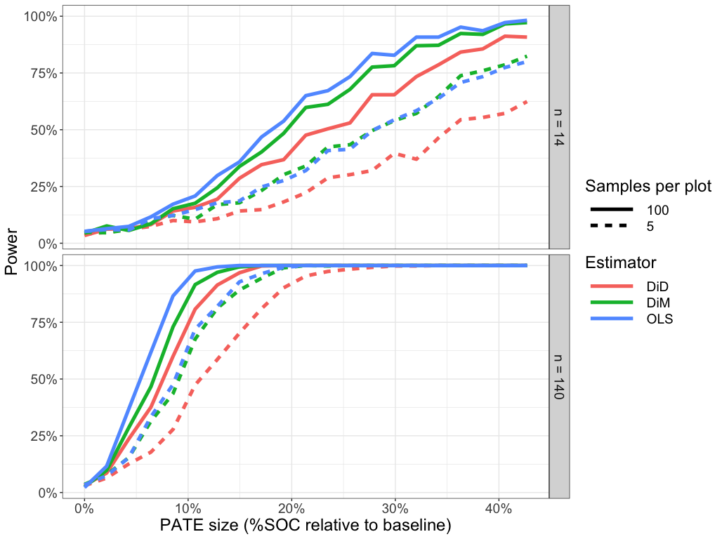
Figure 3: Power (y-axis) of estimators (colors) to detect a range of PATEs (x-axis). The PATE sizes are relative to baseline %SOC (2.34%). The assumed sizes of the balanced RCT appear in the two panels—either 14 or 140 plots—and the numbers of samples per plot—either 5 or 100 samples—appear as the linetypes. Tests were based on checking the lower limit of the 95% Wald confidence intervals for each estimator. The power was then computed as the fraction of times that limit was above 0 (testing a null nypothesis of no effect) over 500 simulations. DiM = difference-in-means; DiD = difference-in-differences; OLS = ordinary least squares; PATE = population average treatment effect.

Moderator estimation:

Results for the causal estimator $\widehat{\beta}_{\mbox{\tiny mod}}$ and the naive estimator of $\beta_{\mbox{\tiny mod}}$ appear in Figure 4. The naive estimator is useless, with a large bias at all sample sizes and confidence intervals that rarely cover the target parameter. The causal estimator works better, but only when both the number of plots in the study and the number of samples per plot are large. It does not achieve its nominal 95% coverage when only 10 plots are enrolled in the study, or when the number of samples per plot is small. With only a few samples plot, the causal estimator suffers from attenuation bias due to plot-level sampling noise. This bias persists even at $n=1000$ and degrades the coverage of designs with only a few samples per plot, as the CI concentrates on a biased parameter estimate.

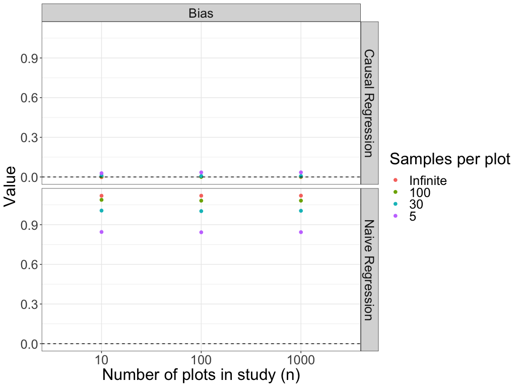
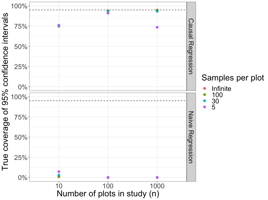
Figure 4: Bias (y-axis; left panels) and 95% confidence interval coverage (y-axis; right panels) of causal (upper panels) and naive (lower panels) estimates of moderator effect $\beta_{\mbox{\tiny mod}}$ of baseline SOC. The number of plots in the study ($n$) appears on the x-axis, and the number of samples per plot is mapped to the color of the points.

Optimal policy estimation:

The average oracle value $\bar{y}(\boldsymbol{z}^{*})$ across the simulated populations was 2.63 TC%. On average the return under the estimated optimal policy $\bar{y}(\hat{\boldsymbol{z}}^{*})$ was 2.61 TC%, with a loss of 0.02 TC% compared to the oracle value. The return under the restricted optimal policy estimate $\bar{y}(\hat{\boldsymbol{z}}_{\mathcal{R}}^{*})$ averaged to 2.50 TC%, with a loss of 0.13 TC%. As expected, the differences were driven primarily by the moderator effect. We observed the relation $\bar{y}(\hat{\boldsymbol{z}}^{*})\geq\bar{y}(\hat{\boldsymbol{z}}_{\mathcal{R}}^{*})$, with the inequality holding strictly when and only when $\beta_{\mbox{\tiny mod}}\neq 0$.

6 Discussion

We provided an integrated review of uncertainties in studies targeting SOC sequestration along with a design-based causal model for estimating treatment effects and optimizing sequestration across a population of interest.

We found that the regression adjusted (OLS) estimator of the population average treatment effect tended to have marginally lower error and confidence interval width than the difference-in-means or difference-in-differences on average across a wide range of simulation settings. The difference-in-differences estimator performed particularly poorly when there was a strong moderating effect of baseline soil organic carbon, as predicted by the saturation hypothesis. Our proposed estimate of the optimal policy using OLS also on the policy of uniformly applying the treatment with the larger average treatment effect estimate, especially when there was treatment effect heterogeneity described by an observed moderator (i.e., sequestration potential). In the rest of this section, we will discuss additional considerations for sequestration studies and policies, limitations of our work here, and directions for future research.

6.1 Other study designs and potential pitfalls

We assumed a very particular study design: a randomized controlled trial (RCT) with units sampled uniformly at random from a broader population of interest. This setup represents an ideal wherein the internal and external validity of all estimates and inferences are rigorously justified by the design alone. Rarely, if ever, is such a design feasible in real-world soil science experiments, but some of the assumptions can be relaxed.

The assumption of simple random sampling into a completely randomized experiment is not necessary: there exist estimators that retain unbiasedness and inferential validity under a much broader range of designs, including non-uniform sampling and assignment, stratification or blocking, rerandomization, and cluster sampling or treatment assignment (Aronow and Middleton, 2013; Imbens and Rubin, 2015; Egami and Hartman, 2023; Li and Ding, 2020). Furthermore, the plots in the experiment may constitute a convenience sample from the larger population or may not be embedded in a population at all. In that case all inferences may be confined to the experiment itself. There is a rich literature on such randomization inference dating back 100 years ago to early agricultural statistics (Neyman, 1923), which continues to flourish today (Lin, 2013; Ding et al., 2019). The internal validity of such experiments is guaranteed by the design alone, but the experiment has no immediate external validity: nothing can be said about a larger population without further assumptions. Section 2.4 described a few ways to support external validity. We emphasize the importance of careful consideration of the population to which results are being extrapolated, and of replicating studies. Replication is the strongest way to establish that causal effects generalize across contexts.

Purely observational studies are more problematic, requiring hypothetical populations and sampling designs premised on unverifiable assumptions. The design-based view of observational causal inference aims to explicitly approximate a hypothetical RCT and to use methods for statistical analysis that are interpretable and transparent so that weaknesses in the study can be easily identified (Rosenbaum, 2002). In contrast, the model-based and Bayesian views tend towards intricate distributional and functional assumptions that are often obscure, strained, and sensitive to misspecifications (Berk and Freedman, 2003).

Some studies may not rely on empirical data at all or may only use empirical data as inputs to a complex mechanistic model. The CENTURY and DAYCENT biogeochemical models (Parton, 1996) are commonly used as part of theoretical studies or to inform policy decisions. For instance, these models have been used to extrapolate measurements over space and time (Silver et al., 2018) and as part of sequestration crediting protocols (Mathers et al., 2023). The reliability of the output of mechanistic models needs to be distinguished from that of experiments. In particular model results are often a weaker form of evidence because their validity is premised on accurately capturing all relevant aspects of the complex, multi-causal, physical mechanisms governing SOC sequestration. The models are obliged to greatly simplify these mechanisms, given that the physics of SOC sequestration (including saturation) remain poorly constrained and highly variable under real-world conditions. The models must be calibrated empirically and tested for their ability to predict SOC changes and causal effects in a wide-range of contexts (Necpálová et al., 2015). Well designed and executed RCTs provide a good source for calibration data.

6.2 A causal view of saturation

The method we developed can be used to furnish empirical evidence for the saturation hypothesis. A large body of past work has failed to provide such evidence, in large part because saturation has not been situated within a causal model, which has led to confusion when analyzing and interpreting the data (Slessarev et al., 2023). In short, investigators have taken baseline SOC $B_{i}$ and followup SOC $Y_{i}$, computed the difference $D_{i}:=Y_{i}-B_{i}$, regressed $D_{i}$ on $B_{i}$, and interpreted a significantly negative regression coefficient as evidence that baseline SOC is negatively associated with change. This is not a meaningful result: the difference between any two independent random variables will be correlated with either one of the original random variables. Slessarev et al. (2023) note this as an instance of regression to the mean, and propose a correction.

Our approach instead suggests formalizing the saturation hypothesis in a causal model, with the phenomenon manifesting either as moderation by baseline SOC or as diminishing returns to inputs. In the binary treatment case, baseline moderation is equivalent to a nonzero value of $\beta_{\mbox{\tiny mod}}$ from Section 4.3. We proposed an estimator of $\beta_{\mbox{\tiny mod}}$ that requires both a large study and a high number of samples per plot to achieve sufficient accuracy, precision, and inferential validity. If only a few samples per plot are taken, the proposed estimator suffers from attenuation bias due to random variability from plot-level sampling. Given these concerns, a binary experiment that accurately estimates the moderating effects of baseline SOC as a proxy for the saturation effect could quickly become prohibitively expensive.

As an alternative, saturation effects could be targeted directly in a dose-response experiment. Specifically, researchers could apply a continuous treatment at varying levels of intensity and test for diminishing returns (Holland-Letz and Kopp-Schneider, 2015; Efron and Feldman, 1991). The aim being to directly estimate curves like those appearing in Figure 2 at the population level. Combining ideas of moderation and dose-response in the design and analysis of studies targeting sequestration is an interesting area of future research, which could shed further light on the saturation hypothesis and improve the efficiency of SOC sequestration policies.

6.3 Costs, optimization, and externalities

In characterizing the available treatment portfolio $\mathcal{P}$, we assumed that the overall cost of a policy was a linear and additive function of the costs of each individual treatment. This assumption creates a linear budget constraint set, which allows the optimal policy to be computed readily: the optimization is a linear program, for which fast algorithms exist at any scale (Karmarkar, 1984).

In many cases, a linear cost model is not appropriate. For example, policies are likely to exhibit economies of scale, so that marginal costs diminish as more plots receive a given treatment. Roughly speaking, diminishing marginal costs would suggest a more parsimonious and balanced treatment regime, where only a few intervention levels are prescribed in relatively equal proportions. In the extreme, it suggests treating all plots the same, i.e., choosing a treatment from $\mathcal{R}$. Furthermore, the real costs of interventions will often depend on geography, especially for treatments involving shipping costs: it is cheaper to spread $x$ amount of an amendment on the same plot than to distribute $x/2$ to two plots (depending on the distance between them).

These considerations could make the optimization much more complex and potentially intractable, even if the population potential outcomes $\{\boldsymbol{y}(\boldsymbol{z})\}_{\boldsymbol{z}\in\mathcal{Z}^{N}}$ were fully known. Brute-force solutions are generally impossible, since they involve enumerating $|\mathcal{Z}|^{N}$ averages $\bar{y}(\boldsymbol{z})$. If geography is a primary concern, the population could be partitioned into $G$ clusters with all plots in a cluster constrained to receive the same treatment, reducing the burden of enumeration to $|\mathcal{Z}|^{G}$. Defining an accurate cost model and finding tractable routines for optimization is an important area for further research.

We also note that the true costs and benefits of different courses of action are not strictly internal to the project. Externalities are generally very difficult if not impossible to account for. Policy costs are not incurred in isolation, but in relation to other existing and potential policies. For example, converting a corn field to native grasses requires resources, but those resources may be diverted from an existing policy (e.g., a corn subsidy). An existing practice may impose a wide range of costs on nature or society—environmental, social, medical, etc—that are difficult to capture in a cost model and compare to a counterfactual action. Many costs are not even quantifiable for an individual, let alone society at large.

6.4 Valid inference with non-normal data, complex target parameters, and sequential designs

The inference methods we proposed in this paper are asymptotically valid: the level of a confidence interval or hypothesis is approximately correct in large samples. How large a given sample must be for the approximation to be close is generally unclear. In our simulations of small studies ($n=10$), Wald-style confidence intervals had true coverage probabilities below their nominal level (90% true vs 95% nominal). Those simulations drew the populations from normal distributions and we expect the coverage would be worse in populations that depart from normality, especially those with strongly varying skew (Stanley et al., 2023). For skew to vary strongly across potential outcome populations, individual treatments effect would need to vary strongly. If the treatment effect is constant, the PATE can be bounded with a guaranteed level using a randomization test (Ding et al., 2016). The constant treatment effect assumption is generally implausible, and is entirely incongruous with the saturation hypothesis. Without that assumption, conservative confidence intervals for the PATE can be constructed by adapting the nonparametric method of Stanley et al. (2023) to the context of an RCT, though that may entail a subsantial loss in power compared to Wald-style intervals. Another option is to target the quantiles of the treatment effects $\{\tau_{i}\}_{i=1}^{N}$ and bound them using the permutation-based method of Caughey et al. (2023). That method may provide additional insight into treatment effect heterogeneity, but changes the subject somewhat since it does not immediately bound average or total sequestration.

Another open problem is inference about the optimal policy $\boldsymbol{z}^{*}$. Earlier we suggested a method that bases the policy decision only on the estimate $\hat{\boldsymbol{z}}^{*}$. However, when the average $\bar{y}(\boldsymbol{z})$ is relatively flat around $\boldsymbol{z}^{*}$ there are many nearly optimal solutions, some of which may have considerably lower cost than $\hat{\boldsymbol{z}}^{*}$. Incorporating the uncertainty of $\hat{\boldsymbol{z}}^{*}$ is thus a valuable goal. To that end, a $(1-\alpha)$ confidence set $\mathcal{C}_{\boldsymbol{z}^{*}}$ might contain all policies $\boldsymbol{z}$ for which the hypothesis

$$H_{0}(\boldsymbol{z}):\max_{\boldsymbol{z}^{\prime}\in\mathcal{P}}\bar{y}(\boldsymbol{z})\geq\bar{y}(\boldsymbol{z}^{\prime})-\epsilon$$

does not reject at level $\alpha$. In other words, $\mathcal{C}_{\boldsymbol{z}^{*}}$ is a set of policies that are probably approximately optimal. The decision maker might then choose the least costly $\boldsymbol{z}$ such that $\boldsymbol{z}\in\mathcal{C}_{\boldsymbol{z}^{*}}$. The setup is similar to the null hypothesis in a bioequivalence problem (Westlake, 1979), inference on optimal average treatment effects (Kasy and Sautmann, 2021), empirical welfare maximization (Kitagawa and Tetenov, 2018), and problems in multiple testing, especially procedures for multiple comparisons with the sample best (Hsu, 1996). Constructing $\mathcal{C}_{\boldsymbol{z}^{*}}$ may be challenging.

Finally, SOC studies could be fruitfully embedded in a sequential design. While myriad details would need to be worked out, in essence the enrollment of plots and their assignment to treatment could take place on a rolling basis, with covariate and outcome data collected regularly over time. Treatments for an individual plot need not be fixed in advance (as a point treatment or pattern over time), but could change in response to measurements or other decisions. The sequential setup is more complex, but more closely aligns with agricultural practice, may improve theoretical frameworks for SOC sequestration policy, and may lead to better practical studies if carefully implemented. Furthermore, some long running agricultural RCTs are best understood as sequentially evolving over time, including examples at Rothamsted Blyth et al. (2023). The relevant literature includes adaptive clinical trials and policy experiments (Pallmann et al., 2018; Kasy and Sautmann, 2021), contextual bandits (Slivkins, 2024; Dudík et al., 2014), reinforcement learning (Sutton and Barto, 1998), and dynamic treatment regimes (Chakraborty and Murphy, 2014). In these settings, recent advances in sequential inference could be leveraged to ensure finite-sample and sequential validity without parametric assumptions (Howard et al., 2021; Ramdas et al., 2023; Waudby-Smith et al., 2024).

6.5 Uncertainties at the policy level

In our review of measurement in Section 2, we did not address uncertainties that arise specifically around policy design. These include additionality, permanence, and leakage. Additionality is often defined to mean that the policy creates SOC sequestration that would not have occurred otherwise, but this generally assumes the effectiveness of interventions (Indigo Agriculture, 2024). Separating the implementation of an action from its effectiveness, we define additionality to mean that the policy stimulates an action that would not have occurred otherwise. For example, when a land manager is paid to stop tilling, they do, and they would not stop if they were not paid: the policy causes the management change to occur. In this respect, additionality is closely related to compliance in the experimental setting, and may be evaluated by considering existing regulatory, financial, physical, and social (dis)incentives to adopt an intervention and by recording information about compliance in a study. While the scientific effects of an intervention are best estimated if there is strong pressure to comply, additionality and policy effects are best estimated if the study reflects the level of compliance that would occur if the policy were actually implemented. That is, while spatial generalization calls for plots to be representative of the population, determining additionality calls for the experimental intervention to be representative of the policy intervention. Additionality of a policy evokes the well-established tension between internal and external validity (Bates and Glennerster, 2017).

Permanence often refers to the longevity of additional sequestered SOC in a population Indigo Agriculture (2024); Smith (2005); Thamo and Pannell (2016), where a return to baseline SOC before 100 years is called a reversal. We differentiate between (a) the permanence of an intervention and (b) the permanence of sequestered SOC. Concept (a) is an additional population-level policy concern and uncertainty, which, like additionality, can be evaluated by monitoring cross-over in a longitudinal study with an externally-valid intervention. Concept (b) is a more complex question that needs to be addressed in the context of the specific intervention and its permanence (i.e. (a)), in addition to scientific knowledge about the SOC trajectory after the intervention is implemented. Long-term studies are particularly useful for furnishing such knowledge, but must be carefully generalized to the population at hand (see Section 2.4).

Finally, leakage refers to the externalities of a particular intervention in terms of its greenhouse effect. An intervention that stores SOC but releases a large amount of methane exhibits leakage (e.g., in flooding fields for conversion to rice cultivation (Minami, 1994; Nitta, 2022), as does an intervention that burns fossil fuel as part of a supply chain (e.g., in transporting compost long-distances (Silver et al., 2018)). Sequestration is storage minus leakage, and need not be positive even when storage is positive. Hence, it is critical to account for leakage through life-cycle assessment, tracking on-farm fossil fuel use, and measuring externalities like methane, nitrous oxide, and nitric oxide production (Minami, 1994; Pilegaard, 2013; Ryals and Silver, 2013). Again, comparison to appropriate counterfactual scenarios is crucial and can be formalized using potential outcomes.

Code

Code implementing our simulations is available at:
https://github.com/spertus/soil-carbon-statistics.

References

- Amelung and Zech [1999] W. Amelung and W. Zech. Minimisation of organic matter disruption during particle-size fractionation of grassland epipedons. Geoderma, 92(1):73–85, September 1999. ISSN 0016-7061. doi: 10.1016/S0016-7061(99)00023-3. URL https://www.sciencedirect.com/science/article/pii/S0016706199000233.
- Aronow and Middleton [2013] P. Aronow and J. Middleton. A class of unbiased estimators of the average treatment effect in randomized experiments. Journal of Causal Inference, 1, 01 2013. doi: 10.1515/jci-2012-0009.
- Bates and Glennerster [2017] M.A. Bates and R. Glennerster. The generalizability puzzle. http://web.archive.org/web/20080207010024/http://www.808multimedia.com/winnt/kernel.htm, 2017. Accessed: 2024-04-19.
- Begill et al. [2023] N. Begill, A. Don, and C. Poeplau. No detectable upper limit of mineral-associated organic carbon in temperate agricultural soils. Global Change Biology, 29(16):4662–4669, 2023. ISSN 1365-2486. doi: 10.1111/gcb.16804. URL https://onlinelibrary.wiley.com/doi/abs/10.1111/gcb.16804. _eprint: https://onlinelibrary.wiley.com/doi/pdf/10.1111/gcb.16804.
- Berk and Freedman [2003] R.A. Berk and D.A. Freedman. Statistical assumptions as empirical commitments. Law, Punishment, and Social Control: Essays in Honor of Sheldon Messinger, pages 234–254, 2003.
- Berry [2004] W. Berry. The Unsettling of America: Culture and Agriculture. Counterpoint, San Francisco, revised edition edition, November 2004. ISBN 978-0-87156-877-9.
- Blyth et al. [2023] F. Blyth, S. Perryman, P. Poulton, M. Glendining, and A. Gregory. Highfield ley-arable experiment cropping sequence 1949-2023. Electronic Rothamsted Archive, Rothamsted Research, 2023. URL https://doi.org/10.23637/rrn1-HLAcrop4923-01.
- Bossio et al. [2020] D.A. Bossio, S.C. Cook-Patton, P.W. Ellis, J. Fargione, J. Sanderman, P. Smith, S. Wood, R.J. Zomer, M. von Unger, I.M. Emmer, and B.W. Griscom. The role of soil carbon in natural climate solutions. Nature Sustainability, 3(5):391–398, May 2020. ISSN 2398-9629. doi: 10.1038/s41893-020-0491-z. URL https://www.nature.com/articles/s41893-020-0491-z. Publisher: Nature Publishing Group.
- Boyle [1661] R. Boyle. The Skeptical Chymist. 1661.
- Brus [2000] D.J. Brus. Using regression models in design-based estimation of spatial means of soil properties. European Journal of Soil Science, 51(1):159–172, 2000. doi: https://doi.org/10.1046/j.1365-2389.2000.00277.x. URL https://bsssjournals.onlinelibrary.wiley.com/doi/abs/10.1046/j.1365-2389.2000.00277.x.
- Caughey et al. [2023] D. Caughey, A. Dafoe, X. Li, and L. Miratrix. Randomisation inference beyond the sharp null: bounded null hypotheses and quantiles of individual treatment effects. Journal of the Royal Statistical Society Series B: Statistical Methodology, 85(5):1471–1491, November 2023. ISSN 1369-7412. doi: 10.1093/jrsssb/qkad080. URL https://doi.org/10.1093/jrsssb/qkad080.
- Chakraborty and Murphy [2014] B. Chakraborty and S.A. Murphy. Dynamic Treatment Regimes. Annual Review of Statistics and Its Application, 1:447–464, 2014. ISSN 2326-8298. doi: 10.1146/annurev-statistics-022513-115553.
- Chenu et al. [2019] C. Chenu, D.A. Angers, P. Barré, D. Derrien, D. Arrouays, and J. Balesdent. Increasing organic stocks in agricultural soils: Knowledge gaps and potential innovations. Soil and Tillage Research, 188:41–52, May 2019. ISSN 0167-1987. doi: 10.1016/j.still.2018.04.011. URL https://www.sciencedirect.com/science/article/pii/S0167198718303738.
- Cochran [1977] W.G. Cochran. Sampling Techniques. John Wiley & Sons, Inc., New York, 3rd edition, 1977.
- Cotrufo et al. [2019] M.F. Cotrufo, M.G. Ranalli, M.L. Haddix, J. Six, and E. Lugato. Soil carbon storage informed by particulate and mineral-associated organic matter. Nature Geoscience, 12(12):989–994, December 2019. ISSN 1752-0908. doi: 10.1038/s41561-019-0484-6. URL https://www.nature.com/articles/s41561-019-0484-6. Publisher: Nature Publishing Group.
- de Gruijter et al. [2016] J.J. de Gruijter, A.B. McBratney, B. Minasny, I. Wheeler, B.P. Malone, and U. Stockmann. Farm-scale soil carbon auditing. Geoderma, 265:120–130, 2016. doi: 10.1016/j.geoderma.2015.11.010.
- Devine et al. [2020] S.M. Devine, A.T. O’Geen, H. Liu, Y. Jin, H.E. Dahlke, R.E. Larsen, and R.A. Dahlgren. Terrain attributes and forage productivity predict catchment-scale soil organic carbon stocks. Geoderma, 368:114286, 2020. doi: 10.1016/j.geoderma.2020.114286.
- Ding et al. [2016] P. Ding, A. Feller, and L. Miratrix. Randomization inference for treatment effect variation. Journal of the Royal Statistical Society. Series B (Statistical Methodology), 78(3):655–671, 2016. ISSN 13697412, 14679868. URL http://www.jstor.org/stable/24775356.
- Ding et al. [2019] P. Ding, A. Feller, and L. Miratrix. Decomposing Treatment Effect Variation. Journal of the American Statistical Association, 114(525):304–317, January 2019. ISSN 0162-1459. doi: 10.1080/01621459.2017.1407322. URL https://doi.org/10.1080/01621459.2017.1407322. Publisher: Taylor & Francis _eprint: https://doi.org/10.1080/01621459.2017.1407322.
- Dudík et al. [2014] M. Dudík, D. Erhan, J. Langford, and L. Li. Doubly Robust Policy Evaluation and Optimization. Statistical Science, 29(4):485–511, 2014. ISSN 0883-4237. URL https://www.jstor.org/stable/43288496. Publisher: Institute of Mathematical Statistics.
- Efron and Feldman [1991] B. Efron and D. Feldman. Compliance as an Explanatory Variable in Clinical Trials. Journal of the American Statistical Association, 86(413):9–17, 1991. ISSN 0162-1459. doi: 10.2307/2289707. URL https://www.jstor.org/stable/2289707. Publisher: [American Statistical Association, Taylor & Francis, Ltd.].
- Egami and Hartman [2023] N. Egami and E. Hartman. Elements of External Validity: Framework, Design, and Analysis. American Political Science Review, 117(3):1070–1088, August 2023. ISSN 0003-0554, 1537-5943. doi: 10.1017/S0003055422000880. URL https://www.cambridge.org/core/journals/american-political-science-review/article/elements-of-external-validity-framework-design-and-analysis/2D0914404C84B3F169732FF1D5E39420.
- Fisher [1925] R.A. Fisher. Statistical methods for research workers. Oliver and Boyd, 1925.
- Freedman [2008a] D.A. Freedman. On regression adjustments in experiments with several treatments. Annals of Applied Statistics, 2(1):176–196, March 2008a. ISSN 1932-6157, 1941-7330. doi: 10.1214/07-AOAS143. URL https://projecteuclid.org/euclid.aoas/1206367817. Publisher: Institute of Mathematical Statistics.
- Freedman [2008b] D.A. Freedman. On regression adjustments to experimental data. Advances in Applied Mathematics, 40(2):180–193, February 2008b. ISSN 0196-8858. doi: 10.1016/j.aam.2006.12.003. URL https://www.sciencedirect.com/science/article/pii/S019688580700005X.
- Georgiou et al. [2022] K. Georgiou, R.B. Jackson, O. Vindušková, R.Z. Abramoff, A. Ahlström, W. Feng, J.W. Harden, A.F.A. Pellegrini, H.W. Polley, J.L. Soong, W.J. Riley, and M.S. Torn. Global stocks and capacity of mineral-associated soil organic carbon. Nature Communications, 13(1):3797, July 2022. ISSN 2041-1723. doi: 10.1038/s41467-022-31540-9. URL https://www.nature.com/articles/s41467-022-31540-9. Publisher: Nature Publishing Group.
- Gorham [1991] E. Gorham. Northern Peatlands: Role in the Carbon Cycle and Probable Responses to Climatic Warming. Ecological Applications, 1(2):182–195, 1991. ISSN 1939-5582. doi: 10.2307/1941811. URL https://onlinelibrary.wiley.com/doi/abs/10.2307/1941811. _eprint: https://onlinelibrary.wiley.com/doi/pdf/10.2307/1941811.
- Hassink [1997] J. Hassink. The capacity of soils to preserve organic C and N by their association with clay and silt particles. Plant and Soil, 191(1):77–87, April 1997. ISSN 1573-5036. doi: 10.1023/A:1004213929699. URL https://doi.org/10.1023/A:1004213929699.
- Holland-Letz and Kopp-Schneider [2015] T. Holland-Letz and A. Kopp-Schneider. Optimal experimental designs for dose–response studies with continuous endpoints. Archives of Toxicology, 89(11):2059–2068, 2015. ISSN 0340-5761. doi: 10.1007/s00204-014-1335-2. URL https://www.ncbi.nlm.nih.gov/pmc/articles/PMC4655015/.
- Howard et al. [2021] S.R. Howard, A. Ramdas, J. McAuliffe, and J.S. Sekhon. Time-uniform, nonparametric, nonasymptotic confidence sequences. The Annals of Statistics, 49(2), apr 2021. doi: 10.1214/20-aos1991. URL https://doi.org/10.1214%2F20-aos1991.
- Hsu [1996] J. Hsu. Multiple Comparisons: Theory and Methods. Chapman and Hall, London, 1996.
- Hurlbert [1984] S.H. Hurlbert. Pseudoreplication and the Design of Ecological Field Experiments. Ecological Monographs, 54(2):187–211, 1984. ISSN 0012-9615. doi: 10.2307/1942661. URL https://www.jstor.org/stable/1942661. Publisher: Ecological Society of America.
- Imbens and Rubin [2015] G.W. Imbens and D.B. Rubin. Causal Inference for Statistics, Social, and Biomedical Sciences: An Introduction. Cambridge University Press, Cambridge, 2015. ISBN 978-0-521-88588-1. doi: 10.1017/CBO9781139025751. URL https://www.cambridge.org/core/books/causal-inference-for-statistics-social-and-biomedical-sciences/71126BE90C58F1A431FE9B2DD07938AB.
- Indigo Agriculture [2024] Indigo Agriculture. Additionality. https://www.indigoag.com, 2024. Accessed: 2024-04-19.
- International Energy Agency [2023] International Energy Agency. Net Zero Roadmap: A Global Pathway to Keep the 1.5 °C Goal in Reach – Analysis, September 2023. URL https://www.iea.org/reports/net-zero-roadmap-a-global-pathway-to-keep-the-15-0c-goal-in-reach.
- Johnston [1849] J.F.W. Johnston. Experimental Agriculture: Being The Results Of Past, And Suggestions For Future Experiments In Scientific And Practical Agriculture. William Blackwell and Sons, 1849. ISBN 978-1-4368-4219-8.
- Karmarkar [1984] N. Karmarkar. A new polynomial time algorithm for linear programming. Combinatorica, 4:373–395, 1984.
- Kasy and Sautmann [2021] M. Kasy and A. Sautmann. Adaptive Treatment Assignment in Experiments for Policy Choice. Econometrica, 89(1):113–132, 2021. ISSN 1468-0262. doi: 10.3982/ECTA17527. URL https://onlinelibrary.wiley.com/doi/abs/10.3982/ECTA17527. _eprint: https://onlinelibrary.wiley.com/doi/pdf/10.3982/ECTA17527.
- Kitagawa and Tetenov [2018] T. Kitagawa and A. Tetenov. Who Should Be Treated? Empirical Welfare Maximization Methods for Treatment Choice. Econometrica, 86(2):591–616, 2018. ISSN 1468-0262. doi: 10.3982/ECTA13288. URL https://onlinelibrary.wiley.com/doi/abs/10.3982/ECTA13288. _eprint: https://onlinelibrary.wiley.com/doi/pdf/10.3982/ECTA13288.
- Kravchenko and Robertson [2011] A.N. Kravchenko and G.P. Robertson. Whole-profile soil carbon stocks: The danger of assuming too much from analyses of too little. Soil Science Society of America Journal, 75(1):235–240, 2011.
- Künzel et al. [2019] S.R. Künzel, J.S. Sekhon, P.J. Bickel, and B. Yu. Metalearners for estimating heterogeneous treatment effects using machine learning. Proceedings of the National Academy of Sciences, 116(10):4156–4165, March 2019. doi: 10.1073/pnas.1804597116. URL https://www.pnas.org/doi/full/10.1073/pnas.1804597116. Publisher: Proceedings of the National Academy of Sciences.
- Lal [2020] R. Lal. Regenerative agriculture for food and climate. Journal of Soil and Water Conservation, 75(5):123A–124A, September 2020. ISSN 0022-4561, 1941-3300. doi: 10.2489/jswc.2020.0620A. URL https://www.jswconline.org/content/75/5/123A. Publisher: Soil and Water Conservation Society Section: A Section.
- Le Quéré et al. [2018] C. Le Quéré, R.M. Andrew, P. Friedlingstein, S. Sitch, J. Hauck, J. Pongratz, P.A. Pickers, J.I. Korsbakken, G.P. Peters, J.G. Canadell, A. Arneth, V.K. Arora, L. Barbero, A. Bastos, L. Bopp, F. Chevallier, L.P. Chini, P. Ciais, S.C. Doney, T. Gkritzalis, D.S. Goll, I. Harris, V. Haverd, F.M. Hoffman, M. Hoppema, R.A. Houghton, G. Hurtt, T. Ilyina, A.K. Jain, T. Johannessen, C.D. Jones, E. Kato, R.F. Keeling, K.K. Goldewijk, P. Landschützer, N. Lefèvre, S. Lienert, Z. Liu, D. Lombardozzi, N. Metzl, D.R. Munro, J.E.M.S. Nabel, S. Nakaoka, C. Neill, A. Olsen, T. Ono, P. Patra, A. Peregon, W. Peters, P. Peylin, B. Pfeil, D. Pierrot, B. Poulter, G. Rehder, L. Resplandy, E. Robertson, M. Rocher, C. Rödenbeck, U. Schuster, J. Schwinger, R. Séférian, I. Skjelvan, T. Steinhoff, A. Sutton, P.P. Tans, H. Tian, B. Tilbrook, F.N. Tubiello, I.T. van der Laan-Luijkx, G.R. van der Werf, N. Viovy, A.P. Walker, A.J. Wiltshire, R. Wright, S. Zaehle, and B. Zheng. Global Carbon Budget 2018. Earth System Science Data, 10(4):2141–2194, December 2018. ISSN 1866-3508. doi: 10.5194/essd-10-2141-2018. URL https://essd.copernicus.org/articles/10/2141/2018/. Publisher: Copernicus GmbH.
- Li and Ding [2020] X. Li and P. Ding. Rerandomization and Regression Adjustment. Journal of the Royal Statistical Society Series B: Statistical Methodology, 82(1):241–268, February 2020. ISSN 1369-7412. doi: 10.1111/rssb.12353. URL https://doi.org/10.1111/rssb.12353.
- Lin [2013] W. Lin. Agnostic notes on regression adjustments to experimental data: Reexamining Freedman’s critique. The Annals of Applied Statistics, 7(1):295 – 318, 2013. doi: 10.1214/12-AOAS583. URL https://doi.org/10.1214/12-AOAS583.
- Mathers et al. [2023] C. Mathers, C.K. Black, B.D. Segal, R.B. Gurung, Y. Zhang, M.J. Easter, S. Williams, M. Motew, E.E. Campbell, C.D. Brummitt, K. Paustian, and A.A. Kumar. Validating DayCent-CR for cropland soil carbon offset reporting at a national scale. Geoderma, 438:116647, October 2023. ISSN 0016-7061. doi: 10.1016/j.geoderma.2023.116647. URL https://www.sciencedirect.com/science/article/pii/S0016706123003245.
- Minami [1994] K. Minami. Methane from rice production. Fertilizer research, 37(3):167–179, October 1994. ISSN 1573-0867. doi: 10.1007/BF00748935. URL https://doi.org/10.1007/BF00748935.
- Minasny et al. [2017] B. Minasny, B.P. Malone, A.B. McBratney, et al. Soil carbon 4 per mille. Geoderma, 292:59–86, 2017.
- Necpálová et al. [2015] M. Necpálová, R.P. Anex, M.N. Fienen, S.J. Del Grosso, M.J. Castellano, J.E. Sawyer, J. Iqbal, J.L. Pantoja, and D.W. Barker. Understanding the DayCent model: Calibration, sensitivity, and identifiability through inverse modeling. Environmental Modelling & Software, 66:110–130, 2015. ISSN 1364-8152. doi: https://doi.org/10.1016/j.envsoft.2014.12.011. URL https://www.sciencedirect.com/science/article/pii/S1364815214003685.
- Neyman [1923] J. Neyman. Sur les applications de la théorie des probabilités aux experiences agricoles: Essai des principes. Roczniki Nauk Rolniczki, 10:1–51, 1923.
- Niermeier-Dohoney [2022] J. Niermeier-Dohoney. “Rusticall chymistry”: Alchemy, saltpeter projects, and experimental fertilizers in seventeenth-century English agriculture. History of Science, 60(4):546–574, December 2022. ISSN 0073-2753. doi: 10.1177/00732753211033159. URL https://doi.org/10.1177/00732753211033159. Publisher: SAGE Publications Ltd.
- Nitta [2022] N. Nitta. Rice farming to restore soil. https://www.earthisland.org/journal/index.php/articles/entry/rice-farming-to-restore-soil/##, 2022. Accessed: 2024-04-19.
- Padarian et al. [2019] J. Padarian, B. Minasny, and A. B. McBratney. Using deep learning to predict soil properties from regional spectral data. Geoderma Regional, 16:e00198, March 2019. ISSN 2352-0094. doi: 10.1016/j.geodrs.2018.e00198. URL http://www.sciencedirect.com/science/article/pii/S2352009418302785.
- Pallmann et al. [2018] P. Pallmann, A.W. Bedding, B. Choodari-Oskooei, M. Dimairo, L. Flight, L.V. Hampson, J. Holmes, A.P. Mander, L. Odondi, M.R. Sydes, S.S. Villar, J.M.S. Wason, C.J. Weir, G.M. Wheeler, C. Yap, and T. Jaki. Adaptive designs in clinical trials: why use them, and how to run and report them. BMC Medicine, 16(1):29, February 2018. ISSN 1741-7015. doi: 10.1186/s12916-018-1017-7. URL https://doi.org/10.1186/s12916-018-1017-7.
- Parton [1996] W.J. Parton. The CENTURY model. In David S. Powlson, Pete Smith, and Jo U. Smith, editors, Evaluation of Soil Organic Matter Models, pages 283–291, Berlin, Heidelberg, 1996. Springer. ISBN 978-3-642-61094-3. doi: 10.1007/978-3-642-61094-3˙23.
- Pilegaard [2013] K. Pilegaard. Processes regulating nitric oxide emissions from soils. Philosophical Transactions of the Royal Society B: Biological Sciences, 368(1621):20130126, July 2013. ISSN 0962-8436. doi: 10.1098/rstb.2013.0126. URL https://www.ncbi.nlm.nih.gov/pmc/articles/PMC3682746/.
- Potash et al. [2023] E. Potash, K. Guan, A.J. Margenot, D.K. Lee, A. Boe, M. Douglass, E. Heaton, C. Jang, V. Jin, N. Li, R. Mitchell, N. Namoi, M. Schmer, S. Wang, and C. Zumpf. Multi-site evaluation of stratified and balanced sampling of soil organic carbon stocks in agricultural fields. Geoderma, 438:116587, 2023. ISSN 0016-7061. doi: https://doi.org/10.1016/j.geoderma.2023.116587. URL https://www.sciencedirect.com/science/article/pii/S0016706123002641.
- Ramdas et al. [2023] A. Ramdas, P. Grünwald, V. Vovk, and G. Shafer. Game-Theoretic Statistics and Safe Anytime-Valid Inference. Statistical Science, 38(4):576 – 601, 2023. doi: 10.1214/23-STS894. URL https://doi.org/10.1214/23-STS894.
- Rosenbaum [2002] P.R. Rosenbaum. Observational Studies. Springer, 2002. URL https://link.springer.com/book/10.1007/978-1-4757-3692-2.
- Ryals and Silver [2013] R. Ryals and W.L. Silver. Effects of organic matter amendments on net primary productivity and greenhouse gas emissions in annual grasslands. Ecological Applications: A Publication of the Ecological Society of America, 23(1):46–59, January 2013. ISSN 1051-0761.
- Sanderman et al. [2017] J. Sanderman, T. Hengl, and G.J. Fiske. Soil carbon debt of 12,000 years of human land use. Proceedings of the National Academy of Sciences, 114(36):9575–9580, September 2017. doi: 10.1073/pnas.1706103114. URL https://www.pnas.org/doi/abs/10.1073/pnas.1706103114. Publisher: Proceedings of the National Academy of Sciences.
- Sanford et al. [2012] G.R. Sanford, J.L. Posner, R.D. Jackson, C.J. Kucharik, J.L. Hedtcke, and T. Lin. Soil carbon lost from Mollisols of the North Central U.S.A. with 20 years of agricultural best management practices. Agriculture, Ecosystems & Environment, 162:68–76, November 2012. ISSN 0167-8809. doi: 10.1016/j.agee.2012.08.011. URL https://www.sciencedirect.com/science/article/pii/S0167880912003222.
- Scott [1999] J.C. Scott. Seeing like a State: How Certain Schemes to Improve the Human Condition Have Failed. Yale University Press, New Haven, CT London, 0 edition edition, February 1999. ISBN 978-0-300-07815-2.
- Silver et al. [2018] W. Silver, S. Vergara, and A. Mayer. Carbon sequestration and greenhouse gas mitigation potential of composting and soil amendments on california’s rangelands. California’s Fourth Climate Change Assessment, 2018. URL https://www.energy.ca.gov/media/2059.
- Six et al. [2024] J. Six, S. Doetterl, M. Laub, C.R. Müller, and M. Van de Broek. The six rights of how and when to test for soil C saturation. SOIL, 10(1):275–279, April 2024. ISSN 2199-3971. doi: 10.5194/soil-10-275-2024. URL https://soil.copernicus.org/articles/10/275/2024/. Publisher: Copernicus GmbH.
- Slessarev et al. [2023] E.W. Slessarev, A. Mayer, C. Kelly, K. Georgiou, J. Pett-Ridge, and E.E. Nuccio. Initial soil organic carbon stocks govern changes in soil carbon: Reality or artifact? Global Change Biology, 29(5):1239–1247, 2023. ISSN 1365-2486. doi: 10.1111/gcb.16491. URL https://onlinelibrary.wiley.com/doi/abs/10.1111/gcb.16491. _eprint: https://onlinelibrary.wiley.com/doi/pdf/10.1111/gcb.16491.
- Slivkins [2024] A. Slivkins. Introduction to Multi-Armed Bandits, April 2024. URL http://arxiv.org/abs/1904.07272. arXiv:1904.07272 [cs, stat].
- Smith [2005] P. Smith. An overview of the permanence of soil organic carbon stocks: influence of direct human-induced, indirect and natural effects. European Journal of Soil Science, 56(5):673–680, 2005. ISSN 1365-2389. doi: 10.1111/j.1365-2389.2005.00708.x. URL https://onlinelibrary.wiley.com/doi/abs/10.1111/j.1365-2389.2005.00708.x. _eprint: https://onlinelibrary.wiley.com/doi/pdf/10.1111/j.1365-2389.2005.00708.x.
- Spertus [2021] J.V. Spertus. Optimal sampling and assay for estimating soil organic carbon. Open Journal of Soil Science, 11:93–121, 2021. doi: 10.4236/ojss.2021.112006.
- Stanford University [2021] Stanford University. Growing climate solutions, October 2021. URL https://news.stanford.edu/2021/10/12/growing-climate-solutions/. Section: Science & Technology.
- Stanley et al. [2023] P. Stanley, J.V. Spertus, J. Chiartas, P.B. Stark, and T. Bowles. Valid inferences about soil carbon in heterogeneous landscapes. Geoderma, 430:116323, February 2023. ISSN 0016-7061. doi: 10.1016/j.geoderma.2022.116323. URL https://www.sciencedirect.com/science/article/pii/S0016706122006309.
- Stewart et al. [2007] C.E. Stewart, K. Paustian, R.T. Conant, A.F. Plante, and J. Six. Soil carbon saturation: concept, evidence and evaluation. Biogeochemistry, 86(1):19–31, October 2007. ISSN 1573-515X. doi: 10.1007/s10533-007-9140-0. URL https://doi.org/10.1007/s10533-007-9140-0.
- Sutton and Barto [1998] R.S. Sutton and A.G. Barto. Reinforcement Learning: An Introduction. Bradford Books, Cambridge, Massachusetts, first edition edition, March 1998. ISBN 978-0-262-19398-6.
- Särndal et al. [1992] C.E. Särndal, B. Swensson, and J. Wretman. Model Assisted Survey Sampling. Springer Series in Statistics. Springer-Verlag, New York, 1992. ISBN 978-0-387-40620-6. URL https://www.springer.com/gp/book/9780387406206.
- Thamo and Pannell [2016] T. Thamo and D.J. Pannell. Challenges in developing effective policy for soil carbon sequestration: perspectives on additionality, leakage, and permanence. Climate Policy, 16(8):973–992, November 2016. ISSN 1469-3062. doi: 10.1080/14693062.2015.1075372. URL https://doi.org/10.1080/14693062.2015.1075372. Publisher: Taylor & Francis _eprint: https://doi.org/10.1080/14693062.2015.1075372.
- Viscarra Rossel et al. [2016] R.A. Viscarra Rossel, D.J. Brus, C. Lobsey, Z. Shi, and G. McLachlan. Baseline estimates of soil organic carbon by proximal sensing: Comparing design-based, model-assisted and model-based inference. Geoderma, 265:152–163, 2016. ISSN 0016-7061. doi: https://doi.org/10.1016/j.geoderma.2015.11.016. URL https://www.sciencedirect.com/science/article/pii/S0016706115301312.
- Viscarra Rossel et al. [2024] R.A. Viscarra Rossel, R. Webster, M. Zhang, Z. Shen, K. Dixon, Y.-P. Wang, and L. Walden. How much organic carbon could the soil store? The carbon sequestration potential of Australian soil. Global Change Biology, 30(1):e17053, 2024. ISSN 1365-2486. doi: 10.1111/gcb.17053. URL https://onlinelibrary.wiley.com/doi/abs/10.1111/gcb.17053. _eprint: https://onlinelibrary.wiley.com/doi/pdf/10.1111/gcb.17053.
- Waudby-Smith et al. [2024] I. Waudby-Smith, L. Wu, A. Ramdas, N. Karampatziakis, and P. Mineiro. Anytime-valid off-policy inference for contextual bandits. ACM / IMS Journal of Data Science, January 2024. doi: 10.1145/3643693. URL https://dl.acm.org/doi/10.1145/3643693.
- Wendt and Hauser [2013] J.W. Wendt and S. Hauser. An equivalent soil mass procedure for monitoring soil organic carbon in multiple soil layers. European Journal of Soil Science, 64(1):58–65, 2013. doi: https://doi.org/10.1111/ejss.12002. URL https://bsssjournals.onlinelibrary.wiley.com/doi/abs/10.1111/ejss.12002.
- Westlake [1979] W. J. Westlake. Statistical Aspects of Comparative Bioavailability Trials. Biometrics, 35(1):273–280, 1979. ISSN 0006-341X. doi: 10.2307/2529949. URL https://www.jstor.org/stable/2529949. Publisher: [Wiley, International Biometric Society].