Cosmology on point: modelling spectroscopic tracer one-point statistics

Abstract

The 1-point matter density probability distribution function (PDF) captures some of the non-Gaussian information lost in standard 2-point statistics. The matter PDF can be well predicted at mildly non-linear scales using large deviations theory. This work extends those predictions to biased tracers like dark matter halos and the galaxies they host. We model the conditional PDF of tracer counts given matter density using a tracer bias and stochasticity model previously used for photometric data. We find accurate parametrisations for tracer bias with a smoothing scale-independent 2-parameter Gaussian Lagrangian bias model and a quadratic shot noise. We relate those bias and stochasticity parameters to the one for the power spectrum and tracer-matter covariances. We validate the model against the Quijote suite of N-body simulations and find excellent agreement for both halo and galaxy density PDFs and their cosmology dependence. We demonstrate the constraining power of the tracer PDFs and their complementarity to power spectra through a Fisher forecast. We focus on the cosmological parameters $\sigma_{8}$ and $\Omega_{m}$ as well as linear bias parameters, finding that the strength of the tracer PDF lies in disentangling tracer bias from cosmology. Our results show promise for applications to spectroscopic clustering data when augmented with a redshift space distortion model.

1 Introduction

The cosmic large-scale structure contains valuable information for understanding the evolution and content of the Universe. Galaxy clustering is one of the primary probes for testing the standard cosmological model and inferring its parameters. The statistical properties of the galaxy distribution observed in spectroscopic surveys are sensitive to the cosmological parameters such as the matter density, the amplitude of matter fluctuations and the dark energy equation of state. Current and upcoming observations from Stage-IV spectroscopic galaxy surveys as for example the Dark Energy Spectroscopic Instrument (Aghamousa et al., 2016, DESI) and Euclid (Laureijs et al., 2011) will increase the statistical power. To realise the maximum potential from the observable data and achieve precise measurements of the cosmological parameters, accurate modelling of the statistics of the galaxy distribution is required.

The galaxy 2-point correlation function and its Fourier transform, the galaxy power spectrum, are the standard tools for extracting cosmological information. Accurate modeling of these statistics requires accounting for non-linear gravitational evolution, baryonic physics, and galaxy bias and stochasticity. Two-point predictions from N-body simulations can explore a wide range of scales but are computationally expensive, limiting their volume and number of realizations and thus sampling the parameter space requires building models (such as halofit, Takahashi et al., 2012) or emulators (see e.g. Knabenhans et al., 2021; Donald-McCann et al., 2022). Alternatively, perturbation theory models like ‘Standard’ Eulerian or Lagrangian Perturbation Theory (Bernardeau et al., 2002), and their extension in terms of the Effective Field Theory of Large-Scale Structure (EFTofLSS, Carrasco et al., 2012; Porto et al., 2014) provide accurate predictions on mildly non-linear scales. This has enabled the full-shape analysis of two-point galaxy clustering from the SDSS-III BOSS data in both real and redshift space (Gil-Marín et al., 2015; Alam et al., 2017; Beutler et al., 2017; Satpathy et al., 2017; Sánchez et al., 2017). The one-loop EFTofLSS including a tracer bias expansion, redshift-space, and the damping of the Baryon-Acoustic Oscillation (BAO) peak has been applied to SDSS-III BOSS data, achieving precise estimates of cosmological parameters such as the matter fluctuation amplitude $\sigma_{8}$, the matter density fraction $\Omega_{m}$ and the Hubble constant $H_{0}$ (D’Amico et al., 2020; Ivanov et al., 2020; Colas et al., 2020). Including higher-order perturbative calculations could allow to probe slightly further into the nonlinear regime.

While 2-point statistics offer valuable insights into the Universe’s density distribution, they do not capture the full non-Gaussian statistical properties of the observed galaxy distribution. To extract the maximum amount of information, additional statistical tools are required to incorporate higher-order correlations. Joint analyses with 2-point and 3-point statistics have demonstrated strong potential for extracting information from available observational data, as that provided from the BOSS survey (D’Amico et al., 2024).

The one-point Probability Density Function (PDF) is a promising beyond two-point statistic to describe the variation of tracer counts in cells across the density distribution. The shape of the PDF depends on a whole series of integrals of higher-order $N$-point correlations, and thus carries significant non-Gaussian information. The underlying dark matter PDF is efficient in extracting information from mildly non-linear scales, improving the estimation of cosmological parameters (Uhlemann et al., 2020). The one-point PDF of finding $N$ objects in spherical cells of fixed radius $R$ is related to the $k$-nearest neighbour statistics (kNN Banerjee and Abel, 2021a), which instead quote the cumulative probability that at fixed $k$, the $k$-th nearest neighbour is at a distance $r$. Simulation-based Fisher forecasts have shown that kNN statistics of matter and massive halos can yield at least a factor of two in constraining power compared to two-point statistics, in line with findings for the PDFs. The one-point matter PDF can be modelled analytically based on large-deviations theory (Bernardeau and Reimberg, 2015; Uhlemann et al., 2015), and has demonstrated to provide accurate predictions for variations in cosmological parameters and neutrino masses (Uhlemann et al., 2020), primordial non-Gaussianity parameters (Friedrich et al., 2020a; Coulton et al., 2023) as well as dynamical dark energy and modified gravity (Cataneo et al., 2022).

Accurately modelling the relationship between observable tracer and predictable dark matter densities is crucial for extracting cosmological information from galaxy clustering. To analyse spectroscopic galaxy survey data using the PDF and take advantage of theoretical predictions for the matter PDF, it is necessary to relate tracer to dark matter densities in cells. Going beyond phenomenological fits (see e.g. Coles and Jones, 1991; Bel et al., 2016; Clerkin et al., 2017; Hurtado-Gil et al., 2017) requires simple yet accurate parametrisations for tracer bias and stochasticity. Simple linear bias and stochasticity models have been applied to extract information from one-point statistics in galaxy survey data. Friedrich et al. (2018); Gruen et al. (2018) constrained cosmology, linear galaxy bias and stochasticity and the matter density skewness from the signals of lensing-in-cells split by photometric galaxy counts, showing that the parameters reproduce the photometric tracer PDFs from DES and SDSS. Repp and Szapudi (2020) constrained linear galaxy bias and $\sigma_{8}$ from SDSS galaxy counts with a simplified bias and redshift-space distortion model along with Poisson shot noise. Leveraging the full power of Stage-IV surveys will require improved modelling of tracer bias and stochasticity which ideally should also be compatible with two-point statistics. Weak lensing is complementary to galaxy clustering and the one-point statistics of the convergence, aperture mass and wavelet $\ell_{1}$-norm have been modelled in Barthelemy et al. (2020); Thiele et al. (2020); Barthelemy et al. (2021); Boyle et al. (2020); Barthelemy et al. (2024); Castiblanco et al. (2024); Sreekanth et al. (2024).

In this work, we extend the matter PDF predictions to include biased tracers. The goal of our study is to use the predictions of the matter PDF together with a simple and accurate model for bias and stochasticity suitable for analyzing spectroscopic survey data.

In Section 2 we briefly review how to obtain predictions for the matter PDF from large-deviations theory and describe how we extract statistics from the Quijote simulation suite. In Section 3 we describe our bias and stochasticity model for one-point statistics and its link to the power spectrum. In Section 4 we validate predictions for the cosmology-dependence of the tracer PDF with simulations and perform a Fisher forecast to assess the constraining power of the tracer PDF compared to the power spectrum. In Section 5 we summarise our results and provide an outlook on future work. Appendix A discusses the tracer-matter connection link between the PDF and the power spectrum. Appendix B presents further validations of our theoretical models and forecasts.

2 Predicted matter PDFs and simulation measurements

2.1 Matter PDF from Large Deviations Theory

Large deviations theory provides a theoretical framework for the calculation of the matter PDF smoothed with a spherical top hat filter in the mildly non-linear regime.

The theory of large deviations reconstructs the probability distribution based on the decay rate of the probabilities with deviations from the mean as some characteristic parameter of the system decreases rapidly to zero (Bernardeau and Reimberg, 2015). A probability density function (PDF) $\mathcal{P}(\delta_{L})$ of some random variable $\delta_{L}$ can be said to satisfy a large deviation principle (LDP) if the limit

$$-\lim_{\epsilon\to 0}\epsilon\ln{\mathcal{P}}(\delta_{L})=\psi(\delta_{L})$$ (1)

exists, where the rate function $\psi(\delta_{L})$ is the leading order term of the log of the density PDF and $\epsilon$ is the driving parameter. The exact form of the PDF can be written as

$${\mathcal{P}}(\delta_{L})=\exp\Big{[}-\frac{\psi(\delta_{L})}{\epsilon}+\mathcal{O}(\epsilon)\Big{]}$$ (2)

with $\mathcal{O}(\epsilon)$ encapsulating all terms above linear in $\epsilon$.

Within the context of 1-point statistics of the cosmic large-scale structure, our random variable comes from smoothing the relative matter density contrast $\delta$ on some scale. In the case of Gaussian initial conditions, the PDF of the linear matter density contrast $\delta_{\mathrm{L}}$ in spheres of radius $r$ is fully specified by a rate function $\psi_{L}(\delta_{L})=\delta_{L}^{2}/2$ and the linear variance at that scale defined by

$$\sigma_{\mathrm{L}}^{2}(r,z)=\int\frac{\mathrm{d}^{3}k}{(2\pi)^{3}}P_{\mathrm{L}}(k,z)W_{\mathrm{3D}}(kr)^{2}\,,$$ (3)

where $W_{\mathrm{3D}}(kr)$ is the spherical top-hat kernel in Fourier space and $P_{\mathrm{L}}(k,z)$ is the linear power spectrum at redshift $z$. The Gaussian PDF can be written as

$${\mathcal{P}_{\rm L}}(\delta_{L})=\frac{1}{\sqrt{2\pi\sigma^{2}_{L}(r,z)}}\exp\left[-\frac{\psi_{\rm L}(\delta_{L})}{\sigma_{L}^{2}(r,z)}\right].$$ (4)

We can see that the PDF is exponentially decreasing with a decay-rate function $\Psi_{L}(\delta_{L};r,z)=\psi_{\rm L}(\delta_{L})/\sigma_{L}^{2}(r,z)$ that is the ratio of the rate function and the variance.

For the nonlinear density contrast $\delta_{m}$ in spheres of radius $R$ we can find an LDP with a rate function

$$\psi_{m}(\delta_{m})=-\lim_{\sigma^{2}\to 0}\sigma^{2}\log\mathcal{P}_{m}(\delta_{m})\,.$$ (5)

This is in the limit of a vanishing non-linear variance $\sigma^{2}=\sigma^{2}_{\rm NL}(R,z)$, which is defined by the non-linear power spectrum in analogy to Equation 3. A consequence of a LDP is the contraction principle which allows us to compute the rate function in terms of that of a different random variable via

$$\psi_{m}(\delta_{m})=\inf_{\delta_{L}:\zeta(\delta_{L})=\delta_{m}}\psi_{L}(\delta_{L})$$ (6)

where $\zeta$ is some continuous mapping. Due to the exponential decay, there will be one dominant, most likely contribution.

The most probable evolution of densities in spheres can be approximated by spherical collapse such that $\zeta(\delta_{m})=\delta_{\mathrm{L}}^{\mathrm{SC}}(\delta_{m})$, where $\delta_{\rm L}$ and $\delta_{m}$ are the linear and nonlinear density contrast with initial and final radii related by $r=R(1+\delta_{m})^{1/3}$ via mass conservation. For the late-time rate function we have that

$$\psi_{m}(\delta_{m})=\frac{\sigma_{\rm L}^{2}(R,z)}{\sigma_{\rm L}^{2}(R(1+\delta_{m})^{1/3},z)}\psi_{\rm L}(\delta_{L}^{\rm SC}(\delta_{m}))$$ (7)

At small variances $\sigma^{2}<1$, the decay rate function can be robustly extrapolated from the rate function by restoring the variance like $\Psi_{m}(\delta_{m};R,z)=\psi_{m}(\delta_{m})/\sigma^{2}_{\rm NL}(R,z)$ (Uhlemann et al., 2015; Bernardeau and Reimberg, 2015). The PDF of the late-time matter density then has exponential behaviour described by

$$\mathcal{P}_{m}(\delta_{m})\sim\exp\left[-\frac{\psi_{m}(\delta_{m})}{\sigma_{\mathrm{NL}}^{2}(R,z)}\right]=\exp\big{[}-\Psi_{m}(\delta_{m};R,z)\big{]}\,.$$ (8)

The prefactor of this expression can be calculated via the cumulant generating function. The scaled cumulant generating function $\varphi_{m}(\lambda)$ (encoding the reduced cumulants) is obtained from the Legendre-Fenchel transform of the rate function

$$\varphi_{m}(\lambda)=\sup_{\delta_{m}}\big{[}\lambda\delta_{m}-\psi{{}_{m}}(\delta_{m})\big{]}\,,$$ (9)

which is then converted to the cumulant generating function by restoring the nonlinear variance

$$\phi_{m}(\lambda;R,z)=\frac{1}{\sigma_{\rm NL}^{2}(R,z)}\ \varphi_{m}\left(\lambda\ \sigma_{\rm NL}^{2}(R,z);R,z\right)\,.$$ (10)

The matter PDF $\mathcal{P}_{m}(\delta_{m})$ is then obtained from an inverse Laplace transform of the cumulant generating function

$$\mathcal{P}_{m}(\delta_{m};R,z)\!=\!\!\int_{-\infty}^{\infty}\frac{\text{d}\lambda}{2\pi}\exp\left[\phi_{m}(i\lambda;R,z)-i\lambda\delta_{m}\right]\ .$$ (11)

It can be approximated well by a suitable saddle point approximation (Uhlemann et al., 2015), but we do not rely on this here. Theoretical predictions used in this work are computed with the above theory using the publicly available code CosMomentum (Friedrich et al., 2020b). While spherical collapse dynamics effectively predict the nonlinear rate function (7) and the generating function of reduced cumulants (9), the non-linear variance entering equations (8) and (10) cannot be accurately inferred. CosMomentum instead predicts this using the non-linear power spectrum $P_{\mathrm{NL}}$ from the revised halofit fitting function from Takahashi et al. (2012). For an alternative approach to computing the PDF with a perturbation theory around spherical collapse following principles of Effective Field Theory see Ivanov et al. (2019); Chudaykin et al. (2023).

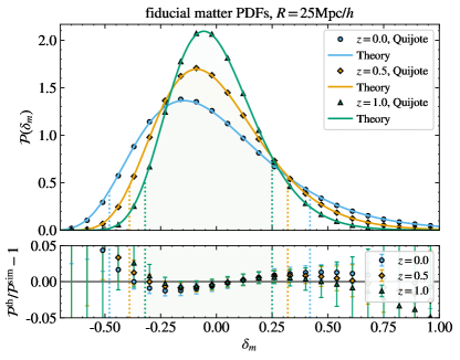
Figure 1: Comparison between matter PDFs extracted from Quijote (data points) with those from theory at smoothing scale $R=25.0$Mpc/$h$ for redshifts $z=0.0,0.5,1.0$. Errors on the residuals in the lower panel are from 100 realisations of the Quijote fiducial cosmology.

2.2 Extracting statistics from the Quijote Simulations

We will refine and validate our theoretical model using measurements from the Quijote simulation suite. The Quijote N-body simulation suite (Villaescusa-Navarro et al., 2019) contains 15,000 independent N-body simulations at a fiducial $\Lambda$CDM cosmology with the parameters: $\sigma_{8}=0.834$, $\Omega_{\rm m}=0.3175$, $\Omega_{\rm b}=0.049$, $n_{s}=0.9624$, $h=0.6711$. Each simulation box has a volume of 1 $(h^{-1}~{}\textrm{Gpc})^{3}$ and traces $512^{3}$ CDM particles. Snapshots are available at five redshifts and we focus on the lowest three $z=0.0,0.5,1.0$ relevant for galaxy surveys. Part of the Quijote simulations were designed with Fisher forecasts in mind, and therefore offer results for a large number of single-parameter variations on their fiducial models. A set of 500 simulations are available for each of the following parameters according to the increment values in Table 4.

2.2.1 Matter PDFs from the Quijote Simulations

Matter PDFs in 99 logarithmic bins from $1+\delta=10^{-2}$ to $10^{2}$ are pre-computed using the publicly-available Pylians3 python library. They rely on a Cloud-in-Cell mass-assignment scheme to deposit the particles on a grid of $512$ and $1024$ cells per side, respectively. The matter density field is then smoothed with a spherical top-hat filter of radius $R=20,25,30$Mpc$/h$ through a multiplication in Fourier space.

Figure 1 compares matter density PDFs at smoothing scale $R=25$Mpc$/h$ and redshifts $z=0.0,0.5$ and 1.0 extracted from Quijote to those computed using CosMomentum. Due to the inaccuracies in predicting the non-linear matter variance in the CosMomentum code, here we rescale $\sigma_{\mathrm{NL}}^{2}$ with the measured value from Quijote . In later sections we will focus our analysis on the bulk of the PDF and thus exclude the highest 10% and lowest {10,5,3}% of density bins for scales $R=20,25,30$Mpc/$h$ respectively, similar to (Uhlemann et al., 2020). The predicted PDFs agree with the measured ones to within 2% around the bulk of the PDF. For a validation of the matter PDF derivatives with respect to cosmological parameters see Appendix B.1.

2.2.2 Halo statistics from the Quijote Simulations

We make use of the Quijote simulations to parameterise the tracer bias and stochasticity required to model the tracer PDF given a matter PDF.

We use Friends-of-Friends (FoF Davis et al., 1985) halo catalogues and extract our statistics for the $N_{h}^{\mathrm{tot}}$ most massive halos for each realisation. The numbers are chosen to be close to the maximum possible in a given halo catalogue (and thus varying across redshifts) to limit the impact of shot noise. Given the size of the simulation box $1$ Gpc$/h$, this corresponds to number densities of $n_{\mathrm{tot}}(z)\sim(1.5-3.9)\times 10^{-4}(h/$Mpc$)^{3}$ for $z\in[0,1]$. Shot noise becomes significant if the average tracer count in cells approaches $\overline{N_{t}}(z,R)\sim 10$, as already happens for $z=1$ and a radius of $R=25$ Mpc$/h$, and more pronounced for $R=20$Mpc$/h$ where $\overline{N_{t}}(z,R)\sim 5$. We picked a fixed number of halos instead of a fixed mass threshold in order to avoid fluctuations of number density across different realisations. For isolating the change of the halo PDF with respect to cosmology, we select a number of halos tuned to leave the halo bias as constant as possible across cosmologies, with values displayed in Table 4. This amounts to changing the minimum halo mass threshold with cosmology to compensate the change in bias due to a larger/smaller number of massive halos, most prominent when changing $\sigma_{8}$.

The processing of the halo catalogues to extract PDFs makes use of the same functions in the Pylians3 library as for the matter PDF. We use the Cloud-in-Cell mass-assignment scheme to deposit the halos on a grid of 500 cells per side. We choose to extract number-weighted PDFs (as opposed to weighting the tracers by their masses) because it most closely corresponds to observable galaxy counts. While a mass-weighting is known to increase the correlation between the matter and tracer densities (see e.g. Seljak et al., 2009; Hamaus et al., 2010; Jee et al., 2012; Uhlemann et al., 2018), our simulation contains only relatively massive halos such that we expect this impact to be small. As number counts are integers, number weighting provides us with an unambiguous binning for the tracer PDF. The halo density field is smoothed with a spherical top-hat filter of radius $R=20,25,30$Mpc$/h$ through a multiplication in harmonic space. The binning for the tracer PDF is adapted so that the bins correspond to multiples of the tracer density contributed by a single tracer in a sphere.

2.2.3 Mock galaxy statistics from the Molino Suite

We also use the Molino suite of galaxy catalogues (Hahn and Villaescusa-Navarro, 2021) suitable for Fisher forecasts. Molino uses the standard Halo Occupation Distribution (HOD) model (Zheng et al., 2007) to populate the Quijote dark matter halo catalogues. The galaxy catalogue contains $\sim 150000$ galaxies and is available for redshift $z=0.0$. The halos are populated according to the probability of a halo of mass $M_{h}$ to host $N_{g}$ number of galaxies. Halos are occupied by central and satellite galaxies, in the standard HOD model the mean number of galaxies is given by their sum

$$\langle N_{g}(M_{h})\rangle=\langle N_{\rm cen}(M_{h})\rangle+\langle N_{\rm sat}(M_{h})\rangle\,.$$ (12a)

The mean occupation of central galaxies is parameterised by

$$\langle N_{\rm cen}(M_{h})\rangle=\frac{1}{2}\left[1-{\rm erf}\left(\frac{\log(M_{h}/M^{\rm min}_{h})}{\sigma_{\log M}}\right)\right]\,,$$ (12b)

where $$M^{\rm min}_{h} \sigma_{\log M} M_{h}$$ is the minimum mass for which half of the halos host a central galaxy above the luminosity threshold and is related to the scatter of the central galaxy luminosity in halos of mass . The mean occupation of satellites follows a power law as

$$\langle N_{\rm sat}(M_{h})\rangle=\langle N_{\rm cen}(M_{h})\rangle\left(\frac{M_{h}-M_{0}}{M_{1}}\right)^{\alpha}\,.$$ (12c)

with $M_{0}$ is the halo mass cut-off for satellite occupation, $M_{1}$ is given such that $M_{h}=M_{0}+M_{1}$ is the typical mass scale for halo to host one satellite and $\alpha$ is the slope at high halo mass. In the Molino suite the fiducial HOD parameters are based on the best-fit for the high luminosity galaxies in the Sloan Digital Sky Survey (SDSS) and are given by $\log(hM_{\rm min}/M_{\odot})=13.65$, $\sigma_{\log M}=0.2$, $\log(hM_{0}/M_{\odot})=14.0$, $\alpha=1.1$ and $\log(hM_{1}/M_{\odot})=14.0$. We follow the same procedure explained above for halos to extract the Molino PDFs for radii $R=25,30$ Mpc$/h$. We use 1000 realisations at the fiducial cosmology and 500 realisations for changes in parameters.

3 Parameterising tracer bias and stochasticity

Various studies have aimed to develop accurate and simple models to capture the one-point tracer-matter density relationship. For example, Uhlemann et al. (2018, 2018) considered mass-weighted subhalo densities and demonstrated that abundance matching using a quadratic mean bias model for log-densities is sufficient to obtain accurate PDFs for tracers in spheres and cylinders. However, neglecting the scatter between galaxy and matter densities fails to capture the stochastic nature of this relationship, which could lead to inaccuracies in more realistic scenarios. The first approach to modelling the non-Poissonian stochasticity between the galaxy field and the matter density field within the PDF framework was presented by Friedrich et al. (2018); Gruen et al. (2018) for projected densities. They explored two models to describe shot noise in conjunction with a linear bias: one with a free parameter that encodes the correlation between the matter and tracer fields, and another using a generalized Poisson distribution with two parameters. Building on this, Friedrich et al. (2022) proposed a quadratic Lagrangian bias expansion for photometric galaxy clustering. They showed that at fixed order the Lagrangian model provides a better fit for the conditional mean than the Eulerian bias expansion. The authors validated their Lagrangian bias expansion against standard consistency relations between Eulerian and Lagrangian perspectives, confirming that their approach is robust and consistent with established two-point statistics. Their analysis also confirms that shot noise deviates from the expected Poisson distribution. The current approach for modelling tracer kNN statistics uses Hybrid Effective Field Theory that combines a perturbative Lagrangian bias model with $N$-body dynamics for the displacements of dark matter and tracers (Banerjee et al., 2022). Here we will take advantage of theoretical predictions for the matter PDF and augment them with a parameterisation of the conditional tracer given matter density PDF relying on suitable bias and stochasticity models.

3.1 Conditional tracer given matter density PDF

Having predicted the matter PDF, we have the first ingredient for the joint PDF of tracer and matter densities, which we can write as a product of the conditional PDF of tracer counts given matter density and the matter PDF

$$\mathcal{P}(N_{t},\delta_{m})=\mathcal{P}(N_{t}|\delta_{m})\mathcal{P}_{m}(\delta_{m})\,.$$ (13)

A tracer density contrast can be defined through $\delta_{t}=N_{t}/\bar{N}_{t}-1$ with the mean number of tracers per cell $\bar{N}_{t}$. Then we can write $\mathcal{P}(N_{t}|\delta_{m})=\mathcal{P}(\delta_{t}|\delta_{m})/\bar{N}_{t}$. In Figure 2 we show the conditional PDF $\mathcal{P}(\delta_{h}|\delta_{m})$ of halo densities in spheres given a certain matter density in spheres. This is extracted from 8000 realisations of the Quijote fiducial cosmology. We clearly see that there is a strong trend and correlation between matter and tracer densities in cells (with correlation coefficients of around $0.9$, see Appendix A.2.2 for details), but also some scatter. We describe this conditional PDF with two ingredients, the conditional mean $\overline{N_{t}}(\delta_{m})=\langle N_{t}|\delta_{m}\rangle$ and the conditional variance $\langle N_{t}^{2}|\delta_{m}\rangle_{c}$ of tracer counts at fixed matter density contrast. The conditional mean – shown by the solid black line – follows the ‘ridge’ of the joint PDF, while the conditional variance captures the scatter around the expectation value – indicated by the dotted lines. For a Poisson distribution, the conditional variance agrees with the conditional mean, and as such we express the model in terms of the ratio $\alpha(\delta_{m})=\langle N_{\rm t}^{2}|\delta_{m}\rangle_{c}/\langle N_{\rm t}|\delta_{m}\rangle$. This model was introduced for density-split statistics in Friedrich et al. (2018); Gruen et al. (2018), generalised in Friedrich et al. (2022) and used for studying HODs in Britt et al. (2024). We apply it to 3D densities for the first time. The conditional distribution of galaxy counts at fixed matter density with a bias model $\overline{N_{\rm t}}(\delta_{m})=\bar{N}_{\rm t}[1+\delta_{t}(\delta_{m})]$ and a shot noise model $\alpha(\delta_{m})$ is given as equation (23) in Friedrich et al. (2020b)

$$\mathcal{P}(N_{\rm t}|\delta_{\rm m}) =\frac{1}{\alpha(\delta_{\rm m})}\exp\left(-\frac{\overline{N}_{\rm t}(\delta_{\rm m})}{\alpha(\delta_{\rm m})}\right)$$ (14)

$$\times\left[\Gamma\left(\frac{N_{\rm t}}{\alpha(\delta_{\mathrm{m}})}+1\right)\right]^{-1}\left(\frac{\overline{N}_{\rm t}(\delta_{\rm m})}{\alpha(\delta_{\rm m})}\right)^{\frac{N_{\rm t}}{\alpha(\delta_{\rm m})}}\,.$$

This can be viewed as a remapping of the continuation of the discrete Poisson distribution where $\alpha=1$

$$\mathcal{P}(N_{t}|\delta_{m})=\mathcal{P}_{\rm P}\left(\tilde{N}_{t}=\!\frac{N_{t}}{\alpha(\delta_{m})};\overline{\tilde{N}_{t}}=\frac{\overline{N_{t}}(\delta_{m})}{\alpha(\delta_{m})}\right)\frac{1}{\alpha(\delta_{m})}\,,$$ (15)

where the normalisation $\alpha(\delta_{m})^{-1}$ comes from the Jacobian $d\tilde{N}_{t}/dN_{t}$ and the Gamma function is the generalisation of the factorial to non-integers. This distribution produces the input conditional mean $\langle N_{t}|\delta_{m}\rangle=\overline{N_{\rm t}}(\delta_{m})$ and the conditional variance $\langle N_{\rm t}^{2}|\delta_{m}\rangle_{c}=\alpha(\delta_{m})\overline{N_{\rm t}}(\delta_{m})$. In the limit of fine sampling $\bar{N}_{t}\rightarrow\infty$, this is well approximated by a Gaussian of mean $\overline{N_{t}}(\delta_{m})$ and variance $\alpha(\delta_{m})\overline{N_{t}}(\delta_{m})$ as we show in more detail in Appendix A.1.

In the spectroscopic case, the relevant observable is the tracer PDF $\mathcal{P}(N_{t})$, which is obtained as a marginal of this joint PDF by integrating over the matter densities

$$\mathcal{P}_{t}(N_{t})=\int\mathcal{P}(N_{t}|\delta_{m})\mathcal{P}_{m}(\delta_{m})d\delta_{m}\,.$$ (16)

In the photometric case, the joint one-point PDF of finding $N$ tracers and a matter overdensity $\delta_{m}$ in cylindrical cells (Friedrich et al., 2022) can be translated to an observable joint PDF between the tracer count and the weak lensing convergence. The joint PDF is also related to the corresponding cross-correlation $(k_{1},k_{2})$-NN statistics (Banerjee and Abel, 2021b), which have been extended to the correlations of tracers with a continuous field in Banerjee and Abel (2023).

3.2 Conditional mean bias model

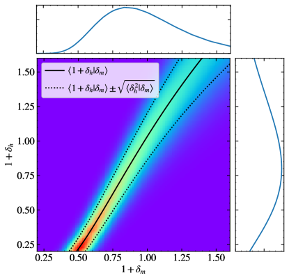
Figure 2: Conditional PDF $\mathcal{P}(\delta_{h}|\delta_{m})$ using 8000 realisations of the Quijote fiducial cosmology at redshift $z=0.0$ and smoothing scale $R=25$Mpc$/h$. The black line shows the conditional mean roughly following the ‘ridge’ of the conditional PDF, while there is also some scatter around the conditional mean, i.e. shot noise (black dashed lines).

The conditional mean encodes a local tracer bias model $\langle N_{t}|\delta_{m}\rangle=\bar{N}_{t}(1+\langle\delta_{t}|\delta_{m}\rangle)$. Figure 3 shows the conditional mean calculated from 500 realisations of the Quijote and Molino fiducial cosmology at redshifts $z=0.0,0.5,1.0$ and $z=0.0$ respectively, and smoothing scale $R=25$Mpc/$h$ (data points). To perform cosmological inference, a simple yet accurate tracer bias parameterisation is desirable. We use local bias models for densities in cells (with a long history including works by Fry and Gaztanaga (1993); Manera and Gaztañaga (2011); Salvador et al. (2019); Repp and Szapudi (2020) and reviews in Bernardeau et al. (2002); Desjacques et al. (2018) ) and their combination with Lagrangian bias principles described in Friedrich et al. (2022).

Of course, tracer formation is in principle non-local, e.g. halos of mass $M$ are expected to form at peaks of the initial density field smoothed over the Lagrangian size $R_{*}(M)=(3M/4\pi)^{1/3}$ (Desjacques et al., 2018). Our tracer selection contains a wide range of halo masses with Lagrangian radii between $1.5$ and $15-25$ Mpc$/h$ (decreasing with increasing redshift) with a mean of around 3 Mpc$/h$. Hence, we can expect the bias to be close to local on our smoothing radii of $R=20-30$ Mpc$/h$.

3.2.1 Eulerian bias models

In a quadratic Eulerian bias model, one would parameterise the tracer bias in terms of the two Eulerian bias parameters $b_{1}^{E}$ and $b_{2}^{E}$,

$$\langle\delta_{h}|\delta_{m}\rangle=b_{1}^{E}\delta_{m}+\frac{b^{E}_{2}}{2}(\delta_{m}^{2}-\sigma_{m}^{2}),$$ (17)

where $\delta_{h/m}$ are measured in the spherical cells and $\sigma^{2}_{m}$ is the matter variance at the same scale that ensures $\langle\delta_{h}\rangle=0$. The bias generally becomes more linear with increasing scale and the linear Eulerian bias $b_{1}^{E}$ approaches the linear bias obtained from the large-scale power spectrum on scales of about $R\sim 60$ Mpc/h (Manera and Gaztañaga, 2011; Friedrich et al., 2022). We find this model to be instructive for a qualitative understanding of the impact of nonlinear bias, but insufficient for a percent-level description of the conditional mean bias.

The Sheth-Mo-Tormen (hereafter SMT) model (Sheth et al., 2001) uses a mass function calculated from an extension to the Press-Schechter excursion set approach (Press and Schechter, 1974) generalised using ellipsoidal collapse equations and fitted to numerical simulations. This allows for statistical predictions of the bias for halos and HOD galaxies. For halos, one can use the SMT model to predict the Eulerian bias parameters $b_{n}^{\rm E}$ as a function of halo mass $M_{h}$. We can then obtain bias parameters for our halo selection from an average over all selected masses weighted by their probability $\mathcal{P}(M_{h})$ via

$$\bar{b}_{{\rm h},n}=\int\mathrm{d}M_{h}b_{n}^{\rm E}(M_{h})\mathcal{P}(M_{h})\,.$$ (18)

In our case, we determine $\mathcal{P}(M_{h})$ from the halo mass function measured in Quijote considering a fixed number of the most massive halos, such that the first halo mass bin $M^{\rm min}_{h}$ is re-weighted according to the leftover number of halos.

tracer	$z$	$b_{1}^{\mathrm{E,fit}}$	$\bar{b}_{1}^{\mathrm{SMT}}$	$b_{2}^{\mathrm{E,fit}}$	$\bar{b}_{2}^{\mathrm{SMT}}$
	0.0	1.56	1.54	-0.56	-0.28
halos	0.5	2.11	2.08	0.38	0.37
	1.0	2.88	2.84	3.11	2.21
galaxies	0.0	2.24	2.44	2.29	2.48

Table 1: Eulerian bias predictions using SMT model and the Quijote halo mass function (18) using the most massive {358364,275253,165107} halos for redshift $z=0,0.5,1$ for halos and $\{156800\}$ galaxies at redshift $z=0.0$ in comparison to Eulerian bias fits of the conditional mean (17) for spheres of radius $R=25$Mpc$/h$.

The bias for HOD galaxies is obtained from a re-weighting given by Zheng et al. (2007)

$$\bar{b}_{{\rm g},n}=\frac{\int\,dM_{h}\langle N_{g}(M_{h})\rangle b_{n}^{\rm E}(M_{h})\mathcal{P}(M_{h})}{\int\,dM_{h}\langle N_{g}(M_{h})\rangle\mathcal{P}(M_{h})}\,,$$ (19)

where the expected number of galaxies per halo mass $\langle N_{g}(M_{h})\rangle$ is determined by the HOD (12). Note that the SMT model is insufficiently precise to be used for real data and is only used here for consistency checks of our analysis.

3.2.2 Lagrangian bias models

Alternatively, one can implement a local Lagrangian bias model at the field level, which is then evaluated along the saddle-point relevant for computing the tracer PDF. This corresponds to a relationship between Eulerian densities in cells with the following functional dependence

$$1\!+\!\langle\delta_{h}|\delta_{m}\rangle=(1+\delta_{m})f_{L}(\delta_{\rm L}(\delta_{m}))-\langle(1+\delta_{m})f_{L}(\delta_{\rm L}(\delta_{m}))\rangle,$$ (20)

where $\delta_{L}(\delta_{m})$ is the inverse spherical collapse mapping relating nonlinear and linear densities and the constant second term is ensuring a zero mean for $\langle\delta_{h}|\delta_{m}\rangle$ that is generated in the computation of the PDF (for details see Friedrich et al., 2022). For a local quadratic Lagrangian bias, we have that

$$f_{L}(\delta_{\rm L})=1+b_{1}^{\rm L}\delta_{\rm L}+\frac{b^{\rm L}_{2}}{2}\delta_{\rm L}^{2}\,.$$ (21)

The Eulerian bias parameters are related to the Lagrangian ones as $b_{1}^{\rm E}\approx 1+b_{1}^{\rm L}$ and $b_{2}^{\rm E}=(1-\nu^{-1})b_{1}^{\rm L}+b_{2}^{\rm L}$, where commonly one assumes $\nu=21/13$ in line with the spherical collapse approximation (Wagner et al., 2015; Lazeyras et al., 2016; Desjacques et al., 2018). For projected densities studied in Friedrich et al. (2022) the quadratic Lagrangian model outperformed the quadratic Eulerian model. However they argued that these findings may not generalise, and indeed we find no improvement here.

Recently, a Gaussian Lagrangian bias model was proposed in (Stücker et al., 2024a, b) which takes the unrenormalised form $\tilde{f}_{\rm L}(\delta_{L})=\exp(\tilde{b}^{\rm G}_{1}\delta_{\rm L}+\tilde{b}^{\rm G}_{2}\delta_{\rm L}^{2}/2)$ with scale-dependent parameters $\tilde{b}_{n}^{\rm G}$. This bias model was designed for the ratio between the Lagrangian galaxy density environment distribution and the background density distribution $f(\delta_{m,\rm L})=\mathcal{P}(\delta_{m,\rm L}|g)/\mathcal{P}(\delta_{m,\rm L})$. For Gaussian initial conditions, $P(\delta_{m,\rm L})$ is Gaussian and empirically, the Lagrangian galaxy density environment distribution is close to a Gaussian as well. This model corresponds to a cumulant- rather than moment-based bias expansion (Stücker et al., 2024b), which matches the spirit of our PDF predictions. A perturbative expansion of the Gaussian bias relation suggests that the leading order terms in this model correspond to a quadratic model with $b_{1}^{\rm L}\approx\tilde{b}_{1}^{\rm G}$ and $b_{2}^{\rm L}\approx(\tilde{b}_{1}^{\rm G})^{2}+\tilde{b}_{2}^{\rm G}$. After renormalisation through a peak-background split, this Gaussian Lagrangian model becomes

$$f_{L}(\delta_{\rm L})=\frac{\exp\left[-\frac{(b_{1}^{\rm G})^{2}}{2b_{2}^{\rm G}}\right]}{\sqrt{1+b_{2}^{\rm G}\sigma_{m}^{2}}}\exp\left[\frac{b_{2}^{\rm G}\left(\frac{b_{1}^{\rm G}}{b_{2}^{\rm G}}+\delta_{L}\right)^{2}}{2(1+b_{2}^{\rm G}\sigma_{m}^{2})}\right]\,,$$ (22)

where the renormalised parameters $b_{n}^{\rm G}$ are now expected to be scale-independent. The scale-dependent parameters are then $\tilde{b}_{n}^{\rm G}=b_{n}^{\rm G}/(1+b_{2}^{\rm G}\sigma_{m}^{2}(R))$. This bias model (22) is fitted to the conditional mean data points and shown as solid lines in Figure 3. The fit is performed in the matter density range corresponding to the bulk of the PDF shown by the shaded regions, with errors calculated from the standard deviation across realisations. We find that the parts of the conditional mean outside of this region do not significantly impact the predicted halo PDF, and so are justifiably excluded from the fit.

The fitted values for the renormalised Gaussian bias for the fiducial cosmology are displayed in the middle two columns of Table 2. As a consequence of the renormalised bias model, there is very little variation between the fitted bias parameters across different smoothing scales. For this reason we perform a fit on all smoothing scales simultaneously ($R=20,25,30$ Mpc/$h$ for halos and $R=25,30$ Mpc/$h$ for galaxies) and these are the values used in Figure 3. The variation across redshift is driven by the formation of halos from high to low redshift such that with an almost fixed minimum halos mass of order $10^{13}M_{\odot}/h$, halos at higher redshift are rarer and thus more biased.

Given a model for the conditional mean of tracer densities given matter densities, one can obtain the cross-covariance between tracer and matter densities as described in Appendix A.2.2.

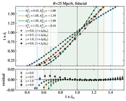
Figure 3: (Upper panel) Conditional mean $\langle\delta_{t}|\delta_{m}\rangle$ from Quijote matter and halos and Molino galaxies in spheres of radius $R$ (data points) along with a renormalised Gaussian Lagrangian bias fit (22) of $b_{1}^{\mathrm{G}}$ and $b_{2}^{\mathrm{G}}$ (solid lines). (Lower panel) Residual defined as $(1+\langle\delta_{t}|\delta_{m}\rangle_{\rm fit})/(1+\langle\delta_{t}|\delta_{m}\rangle_{\rm sim})-1$ with error bars indicating the standard deviation across 500 realisations.

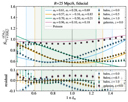
Figure 4: Quadratic shot noise (24) fitted to the ratio of the conditional variance to the conditional mean of the halo counts in the shaded regions corresponding to each redshift, and the error bars are calculated from 500 of the fiducial cosmology.

3.3 Conditional variance stochasticity model

The conditional variance models the tracer stochasticity or shot noise. We focus on the ratio

$$\alpha(\delta_{m})=\frac{\langle N_{t}^{2}|\delta_{m}\rangle_{c}}{\langle N_{t}|\delta_{m}\rangle}=\frac{\bar{N}_{t}\langle\delta_{t}^{2}|\delta_{m}\rangle_{c}}{1+\langle\delta_{t}|\delta_{m}\rangle}\,,$$ (23)

which would be unity in the case of Poisson sampling and was already used in the photometric clustering case in Friedrich et al. (2018, 2022). As before, density contrasts $\delta_{t/m}$ are within spheres of radius $R$. Note that this shot noise is the stochasticity with respect to a deterministic local bias model described by the conditional mean $\langle\delta_{h}|\delta_{m}\rangle$. Figure 4 shows this ratio at redshifts $z=0.0,0.5,1.0$ for halos and $z=0.0$ for galaxies, which possesses a clear deviation from the Poissonian expectation including a density-dependence. We parameterise the shot noise ratio with a quadratic density-dependence

$$\alpha(\delta_{m})=\alpha_{0}+\alpha_{1}\delta_{m}+\alpha_{2}\delta_{m}^{2}\,.$$ (24)

As before, the fits are performed using the data points and errors extracted from the Quijote and Molino realisations in the shaded regions and the results are shown as solid lines.

tracer	$z$	$R$	$b_{1}^{\mathrm{G}}$	$b_{2}^{\mathrm{G}}$	$\alpha_{0}$	$\alpha_{1}$	$\alpha_{2}$
		20	0.449	-0.991	0.57	0.22	0.8
halos	0.0	25	0.443	-1.019	0.65	0.42	0.82
		30	0.440	-1.018	0.72	0.56	0.76
		All	0.446	-1.001	0.61	0.28	0.69
		20	1.058	-1.381	0.56	-0.19	0.87
halos	0.5	25	1.051	-1.399	0.58	-0.08	1.06
		30	1.045	-1.396	0.61	-0.0	1.17
		All	1.053	-1.390	0.57	-0.16	0.83
		20	1.962	-1.87	0.69	-0.49	0.23
halos	1.0	25	1.946	-1.918	0.69	-0.51	0.52
		30	1.934	-1.935	0.71	-0.51	0.74
		All	1.951	-1.895	0.70	-0.50	0.21
		25	1.54	-0.34	0.92	0.09	0.31
galaxies	0.0	30	1.51	-0.30	1.02	0.13	0.32
		All	1.52	-0.34	0.96	0.10	0.18

Table 2: Values of renormalised Gaussian Lagrangian tracer bias $b_{n}^{\mathrm{G}}$ and quadratic shot noise $\alpha_{n}$ parameters at different redshifts and smoothing scales $R\;[\mathrm{Mpc}/h$] from fits to the conditional mean and variance for the fiducial cosmology.

The fitted values for the shot noise parameters for the fiducial cosmology are displayed in the last three columns of Table 2. The conditional variances for different sphere radii possess a moderate scale dependence. Therefore, we perform the fits for the tracer stochasticity for all smoothing scales simultaneously.

While the modelling of stochasticity for the PDF and the power spectrum follow somewhat different principles, we discuss their connection in Appendix A.2.2. When using a fitted bias function, it might be beneficial to modify the defined ratio in equation (23) as follows

$$\alpha_{\rm fit}(\delta_{m})=\frac{\bar{N}_{t}\langle\delta_{t}^{2}|\delta_{m}\rangle}{1+\langle\delta_{t}|\delta_{m}\rangle_{\rm fit}}=\alpha(\delta_{m})\frac{1+\langle\delta_{t}|\delta_{m}\rangle}{1+\langle\delta_{t}|\delta_{m}\rangle_{\rm fit}}\,.$$ (25)

to avoid a propagation of inaccuracies in fitting the conditional mean to the conditional variance. In practice we find that thanks to the good accuracy of the Gaussian Lagrangian bias parametrisation this makes little difference to the accuracy of the halo PDFs at the fiducial cosmology.

3.4 Validating the fiducial tracer PDFs

We compute theoretical predictions for the PDF using the publicly available code CosMomentum (Friedrich et al., 2020b) that implements equation (16). We calculate the theory PDFs with a tracer density $n_{h}=N_{h}^{\mathrm{tot}}\times(\mathrm{Gpc}/h)^{-3}$ given values from the first row of Table 4 and with $\Lambda$CDM cosmological parameters corresponding to the Quijote fiducial cosmology.

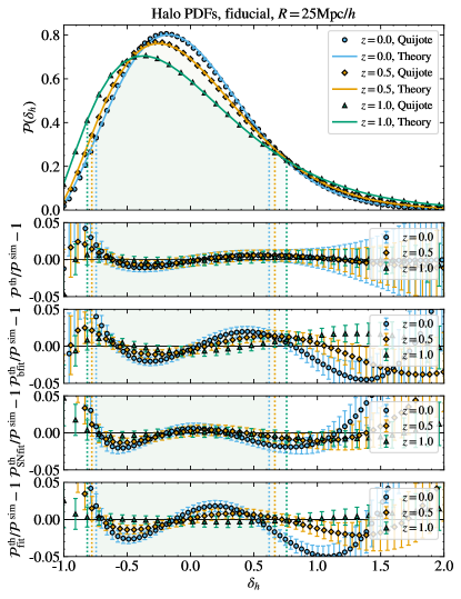
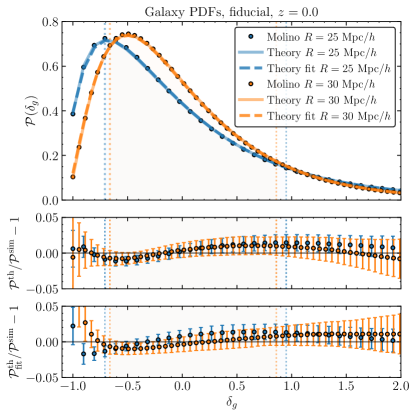
Figure 5: [Upper panel] Comparison of halo PDFs from Quijote (data points) and predictions using the Gaussian Lagrangian bias and quadratic shot noise fits (solid lines) at smoothing scale $R=25$ Mpc/$h$ for redshifts $z=0.0,0.5,1.0$. [Lower panels] Residuals using full functional forms of the bias and shot noise, fitted bias, fitted shot noise, and fitted bias and shot noise. Errors are the standard deviation of 15000 fiducial Quijote realisations.

Figure 6: [Upper panel] Comparison of Galaxy PDFs from Molino (data points) and theory using the full functional forms of bias and shot noise (solid line) or their fits (dashed line) at smoothing scales $R=25,30$ Mpc/$h$ for redshift $z=0.0$. [Lower panels] Residuals of the theory with full functional forms or using the bias and shot noise fits.

Figure 6 compares the halo PDFs from theory with those extracted from simulations. In contrast with the matter PDFs in Figure 1, the halo PDFs become more non-Gaussian with a higher variance as the redshift increases. As can be seen from Table 2, halos are increasingly biased at higher redshift. The variance of the halo density field scales with the linear bias like $\sigma_{h}^{2}\sim b^{2}\sigma_{m}^{2}$ so although the matter variance still decreases, this increasing bias leads to a mildly increasing halo variance with redshift. As for the matter PDF in Figure 1, we focus our analysis on the bulk of the PDF and thus exclude the highest 10% and lowest {10,5,3}% of density bins for scales $R=20,25,30$Mpc$/h$ respectively. When we use the full functional forms of the conditional mean and variance first residual panel, the residual of the halo PDF has a very similar profile to that of the matter PDF, indicating that the inaccuracy of our theoretical model stems from the imperfections in the matter PDF theory. We also show a theoretical model with the renormalised Gaussian Lagrangian bias parameterisation (22) but the full functional form of the stochasticity (second residual panel), which shows increased residuals at lower redshifts indicating the limitations of the two-parameter bias model. When using the full functional form of the bias and the quadratic shot noise model (24), again residuals increase with redshift but with slightly smaller amplitude indicating limitations of the three-parameter stochasticity model (third residual panel). Finally, when using both parameterisations of bias and stochasticity (lower panel) residuals from the two middle residual panels combine. Since the renormalised bias fits result in very little variation of $b_{1}^{\mathrm{G}}$ and $b_{2}^{\mathrm{G}}$ across smoothing scales, we do a joint fit across three smoothing scales and use the same values for all scales. The third and fourth panels show the residuals when using the parameterised bias and the full shot noise, and vice versa. While the parameterisation of both bias and shot noise increases the errors, but we still see good agreement, with the residual plots showing difference of less than 3% around the bulk of the PDF.

The method illustrated for the halos is also applicable to a galaxy sample. In Figure 6 we compare the measured PDF from the Molino mock galaxy catalogues with the theory predictions from CosMomentum. We present PDF prediction computed by using the full functional form of the conditional mean and conditional variance (Theory) and using the renormalised Gaussian Lagrangian bias and the quadratic shot noise fits (Theory fit). In both cases the theory predicts the measured galaxy PDF to within 3% accuracy around the bulk of the PDF as shown in the middle and lower panel respectively. We note that the galaxy PDF presents a higher degree of non-Gaussianity compared to the halo PDF at the same redshift due to its larger linear bias.

3.5 Power spectrum bias and stochasticity

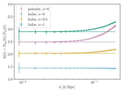
Figure 7: Halo and galaxy bias $b(k)$ obtained from the ratio of the cross-power spectrum and the matter power spectrum (data points with error bars) along with the corresponding quadratic fit (26) (solid lines) and its linear part (dashed lines).

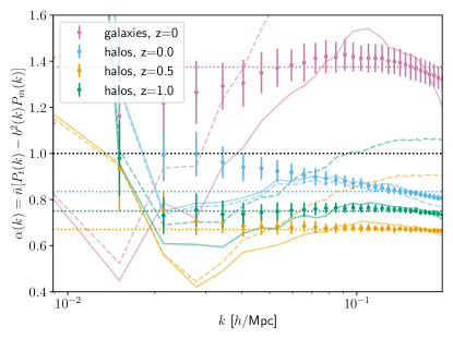
Figure 8: Halo and galaxy shot noise $\alpha(k)$ from equation (27) obtained from the cross-power spectra (data points) or the modelled bias $b(k)$ with quadratic fits (26) (faint solid lines) and their linear parts (faint dashed lines). We also show white noise fits at constant $\bar{\alpha}_{0}$ (coloured dotted lines) which deviate from the Poisson expectation (black dotted).

tracer	$z$	$b_{1}^{\rm E}$	$b_{2,k^{2}}^{\rm E}$	$\bar{\alpha}_{0}$
	0.0	1.44	-0.01	0.83
halos	0.5	2.03	0.17	0.67
	1.0	2.89	0.41	0.75
galaxies	0.0	2.46	0.67	1.29

Table 3: Values of the fitted Eulerian bias (26) and stochasticity (27) parameters for the tracer power spectra.

Following our approach for the tracer PDF, we want to adopt a description of bias and shot noise that is independent of the theoretical modelling for dark matter. Hence, we choose to determine the functional forms of the bias and the shot noise for the tracer power spectrum from the tracer-matter cross-power spectra. The linear, but potentially scale-dependent bias is obtained as the ratio of the cross-power spectrum to the matter power spectrum

$$b(k)=\frac{P_{tm}(k)}{P_{m}(k)}\approx b_{1}+b_{2,k^{2}}\frac{k^{2}}{k_{\rm max}^{2}}\,,$$ (26)

shown in Figure 7 for the fiducial cosmology with fit values given in Table 3. We find that the linear Eulerian bias parameter $b_{1}^{\rm E}$ is close to the expectation from the Gaussian Lagrangian bias from the conditional mean $b_{1}\simeq 1+b_{1}^{\rm G}$. We picked a simple parameterisation for linear bias beyond $b_{1}$ that is proportional to $k^{2}$ (in analogy to the case of projected densities Friedrich et al., 2022) and a reference scale at our $k_{\rm max}=0.2h/$Mpc. Scale-dependent bias of this form can originate from the nonlinear and non-local nature of tracer formation. We briefly touch on quadratic bias terms in Appendix A.2.2. Halos form preferentially at peaks of the initial density field leading to a term of the form $(kR_{\rm pk})^{2}$ with some characteristic peak scale $R_{\rm pk}$ (Desjacques et al., 2018). As we consider a selection of halos with a wide range of masses, which form not only on different scales, but also at different times, it is hard to predict the combined value for $b_{2,k^{2}}$. We suspect that larger values of $b_{2,k^{2}}$ for the halo samples at higher redshift and the mock galaxies are responsible for the slight scale dependence of the renormalised Gaussian Lagrangian bias parameters $b_{1}^{\rm G}$ we obtained from a fitting the conditional mean that were summarised in Table 2.

We can define a shot noise with respect to the linear bias as

$$\frac{\alpha(k)}{\bar{n}}=P_{t}(k)-b^{2}(k)P_{m}(k)\approx\frac{\bar{\alpha}_{0}}{\bar{n}}\,,$$ (27)

with $b(k)$ from equation (26). The result is shown in Figure 8 for halos and galaxies. Fitting a constant $\bar{\alpha}_{0}$ corresponding to white noise (coloured dotted lines) leads to decent agreement on the more nonlinear scales where the shot noise term is most important, while it fails to fit the larger more linear scales. We quote values for the fitted stochasticity parameters at the fiducial cosmology in Table 3. Note that (overly) simplistic choices for the bias function can change the obtained shot noise. This happens for smaller $k$ ranges for our two-parameter scale-dependent bias fit (26) (translucent solid lines) and more significantly for a scale-independent bias with the same $b_{1}$ (translucent dashed lines) for which $\alpha(k)$ increases significantly for larger $k$. If our linear scale-dependent bias model (26) would be exact, the shot noise obtained from a scale-independent modelling would change as $\Delta\alpha(k_{\rm max})=b_{2,k^{2}}(2b_{1}+b_{2,k^{2}})\bar{n}P_{m}(k_{\rm max})$. The amplitude of the power spectrum shot noise agrees well with a shot noise amplitude defined using cross-covariances of the smoothed density (51) around the relevant scales $k\sim\pi R^{-1}$, which can be related to the $\alpha_{n}$ parameters describing the conditional variance as described in Appendix A.2.2.

To test the convergence of the simulated derivatives for the mildly nonlinear halo power spectrum, we adopt a simplistic model for the tracer power spectrum in terms of the nonlinear matter power spectrum

$$P_{t}(k,z)=b(k)^{2}P_{m}(k,z)+\frac{\alpha(k)}{\bar{n}(z)}\,,$$ (28)

where we use a quadratic model for $b(k)$ following equation (26) with two Eulerian bias parameters $b_{1}$ and $b_{2,k^{2}}$ and a constant shot noise amplitude $\alpha(k)=\bar{\alpha}_{0}$ in relation to the inverse of the number density $\bar{n}(z)$ as expected for Poisson sampling. We will use halofit predictions for the non-linear matter power spectrum, which also determine the non-linear matter variance in the PDF predictions. On large scales, the matter power spectrum will reduce to the linear prediction. In Appendix B.4 we show that despite the simplicity of our model, the fiducial signal is well reproduced as shown in Figure 21. Additionally, the derivatives with respect to cosmological parameters shown in Figure 23 are well captured leading to decent agreement between the Fisher contours. Having validated our predictions, we will later use them to forecast the constraining power at fixed tracer number density and bias.

4 Probing cosmology with tracer PDFs

In this section we determine the sensitivity of the tracer PDF to changing cosmological and bias parameters. We will focus on $\sigma_{8}$ and $\Omega_{m}$ as cosmological parameters and one effective bias parameter $\beta$ per redshift. As described in the previous section, the tracer PDF (16) depends on the underlying cosmology that determines the matter PDF (11), and additionally on the conditional PDF of tracer density given matter density. We build the conditional PDF (14) from two functions: the mean tracer count given matter density $\overline{N_{t}}(\delta_{m})=\bar{N}_{t}(1+\langle\delta_{t}|\delta_{m}\rangle)$ and stochasticity captured through the ratio $\alpha(\delta_{m})=\langle N_{t}^{2}|\delta_{m}\rangle_{c}/\overline{N_{\rm t}}(\delta_{m})$. The mean number of tracers per cell is determined by the tracer number density $\bar{n}$ and the cell radius $R$ as $\bar{N}_{t}=4\pi R^{3}\bar{n}/3$. We have described effective parameterisations for the two crucial functions in terms of two Gaussian Lagrangian bias parameters $b_{n}^{\rm G}$ and three shot noise parameters $\alpha_{n}$. From theory arguments we know that the halo bias (18) and HOD-based galaxy bias (19) carry a cosmology dependence through the halo mass function $\mathcal{P}(M_{h})$. Similarly, the total number density of tracers will be cosmology-dependent. We do not seek to extract information from the halo mass function through the tracer PDF here, and hence decide to select tracers across different cosmologies in a way that keeps the tracer bias fixed. This comes at the price of changing number densities, but we mitigate the main impact of this by looking at PDFs of tracer density contrasts $\mathcal{P}_{\delta_{t}}(\delta_{t})=\bar{N}_{t}\mathcal{P}_{t}(N_{t})$.

4.1 Cosmology & mass dependence of bias

We extract tracer PDFs in such a way as to leave the bias as constant as possible by tailoring the number of halos selected for each cosmology, i.e. selecting the only the most massive $N_{h}^{\mathrm{tot}}$ halos. The numbers used to achieve this for each cosmology and redshift are shown in Table 4.

tracer	$z$	fiducial	$\sigma_{8}^{-}$	$\sigma_{8}^{+}$	$\Omega_{m}^{-}$	$\Omega_{m}^{+}$
halos	$0.0$	358364	390000	329930	361020	355876
halos	$0.5$	275253	300000	252965	269741	276134
halos	$1.0$	165107	180000	151694	162795	167293
galaxies	$0.0$	156800	156316	157189	151641	162033

Table 4: Number of tracers $N_{t}$ selected to leave bias constant across cosmology.

To obtain the values for the $N_{h}$ cut across different cosmologies we follow the SMT bias predictions (18) relying on the cosmology-dependent halo mass function $\mathcal{P}(M_{h})$ measured from the simulations. Since fine-tuning $\bar{b}_{n}$ by changing the minimum mass $M_{h}^{\rm min}$ is challenging due to the wide bins of the halo mass function (set by the mass resolution), we instead select a total number $N_{h}^{\mathrm{tot}}$ which we use to cut the mass function by emptying the lowest required mass bin by the necessary number of halos such that the integral evaluates to the desired bias value. One can then find the value of $N_{h}^{\mathrm{tot}}$ that minimises the difference between $\bar{b}_{1}$ and the desired linear bias of the fiducial cosmology. Note that if we kept the selected number of halos fixed across cosmologies this would significantly alter the shape of the derivatives. For example, a change in $\sigma_{8}$ would cause the matter variance and the linear bias to change in opposite directions such that that the halo variance $\sigma_{h}^{2}\approx b_{1}^{2}\sigma_{m}^{2}$ remains almost unchanged.

Similarly, to keep the linear galaxy bias fixed across different cosmologies, we follow the procedure outlined above. We extract the quantity $\langle N_{g}(M_{h})\rangle P(M_{h})$ from the Molino suite and search for the number of galaxies that minimises the difference between the measured and the fiducial bias $\bar{b}_{{\rm g},1}$. Once the number of galaxies is determined for each cosmology the galaxy PDF is measured from the Molino suite considering the corresponding number of galaxies in the most massive halos. As we consider the most massive halos this selection includes most of the satellite galaxies. We measure the conditional mean and conditional variance of galaxy counts given matter density from the Molino suite, considering the corresponding number of galaxies for each cosmology.

4.2 Response to cosmology and tracer selection

We want to quantify the response of the tracer density PDF to changes in cosmology and the tracer selection. While we extract the PDFs of the tracer number count $\mathcal{P}(N_{t})$, we convert them to PDFs of the tracer density contrast $\mathcal{P}(\delta_{t})$ to avoid extracting cosmological information from the variation of the tracer number density across cosmologies. To this end, we compute the parameter derivatives from finite differences between the PDFs of incremented and decremented parameters $\theta^{\pm}$ , i.e.

$$\frac{\partial\mathcal{P}}{\partial\theta}=\frac{\mathcal{P}(\theta^{+})-\mathcal{P}(\theta^{-})}{\theta^{+}-\theta^{-}}\,.$$ (29)

The simulations are with symmetric increments such that $\theta^{\pm}=\theta_{\rm fid}\pm\Delta\theta$ with $\Delta\sigma_{8}=0.015$ and $\Delta\Omega_{m}=0.01$.

We vary the tracer selection at fixed number density by changing the fiducial selection of the most massive halos to the least massive halos. We parameterise this change by introducing the parameter $\beta$ as the fractional difference from the fiducial value of the linear Eulerian bias parameter

$$\beta=\frac{b_{1}}{b_{1}^{\mathrm{fid}}}-1.$$ (30)

with values of $b_{1}$ taken from the power spectrum fits described in Section 3.5, which closely resemble the Eulerian linear bias for the PDF. The $\beta$ derivative is a one-sided derivative representing the effect of changing the whole conditional PDF $\mathcal{P}(\delta_{t}|\delta_{m})$ parameterised through the bias and the shot noise at fixed cosmology. For the simulation derivatives it is calculated by extracting PDFs not with the $N_{t}^{\mathrm{tot}}$ most massive halos/galaxies as described in the previous subsection, but instead prioritising lower mass objects. In practice this means taking the $N_{h}^{\mathrm{tot}}$ lowest mass halos or $N_{g}^{\mathrm{tot}}$ galaxies where satellites are preferentially selected. We then take the derivative to be

$$\frac{\partial\mathcal{P}}{\partial\beta}=\frac{\mathcal{P}(\beta^{\mathrm{fid}})-\mathcal{P}(\mathrm{\beta^{-}})}{\beta^{\mathrm{fid}}-\beta^{-}}\,.$$ (31)

		$b_{1}^{\mathrm{G}}(\beta)$		$b_{2}^{\mathrm{G}}(\beta)$		$\alpha_{0}(\beta)$		$\alpha_{1}(\beta)$		$\alpha_{2}(\beta)$		$b_{1}^{\mathrm{E}}(\beta)$		$b_{2,k^{2}}^{\mathrm{E}}(\beta)$		$\bar{\alpha}_{0}(\beta)$
tracers	$z$	$\beta^{\rm fid}$	$\beta^{-}$	$\beta^{\rm fid}$	$\beta^{-}$	$\beta^{\rm fid}$	$\beta^{-}$	$\beta^{\rm fid}$	$\beta^{-}$	$\beta^{\rm fid}$	$\beta^{-}$	$\beta^{\rm fid}$	$\beta^{-}$	$\beta^{\rm fid}$	$\beta^{-}$	$\beta^{\rm fid}$	$\beta^{-}$
	0.0	0.446	0.277	-1.001	-1.068	0.61	0.88	0.28	0.63	0.69	0.27	1.44	1.28	-0.01	-0.09	0.83	1.14
halos	0.5	1.053	0.842	-1.390	-1.519	0.57	0.75	-0.16	0.27	0.83	0.70	2.03	1.84	0.17	0.07	0.67	0.91
	1.0	1.951	1.613	-1.895	-2.082	0.70	0.80	-0.50	-0.09	0.21	0.51	2.89	2.59	0.41	0.26	0.75	0.89
galaxies	0.0	1.524	1.409	-0.344	-0.348	0.96	0.87	0.09	0.02	0.19	0.42	2.46	2.36	0.67	0.60	1.29	1.15

Table 5: Values of PDF tracer bias and stochasticity parameters from a joint fit of all smoothing scales along with power spectrum bias and stochasticity, using the fiducial and modified tracer selection prioritising lower halo masses and satellite galaxies, respectively.

The changes in the bias and shot noise parameters as a response to this tracer selection are shown in Table 5. While this results in larger step sizes than is ideal for the use of finite difference derivatives, we only use this to cross-validate theory and simulations and use the same step size for both.

The relevant PDFs $\mathcal{P}(\theta^{\pm})$ can be computed in CosMomentum from the same model described previously and tracer power spectra can be constructed following our model (28). Since we constructed halo samples from Quijote in such a way that the bias does not significantly change across cosmology, the fiducial bias can be used for all cosmologies. Similarly, the shot noise can be regarded as effectively constant across cosmologies, although it does still change slightly. Then the only changes going into the theory go into the underlying matter field and a change in tracer density $n_{h}$ coming from the $N_{h}^{\mathrm{tot}}$ cuts in Table 4. Since we consider PDFs of density contrasts rather than number counts, the slight changes do not significantly change the derivatives.

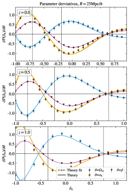
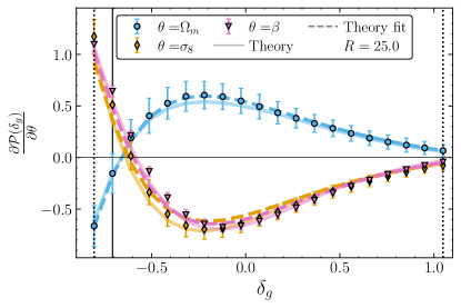
Figure 9: Halo PDF derivatives with respect to the cosmological parameters from Quijote (data points) and theory (solid lines) and parameterised theory (dashed lines) using the renormalised Gaussian Lagrangian bias and quadratic snot noise combined smoothing scale fits. Derivatives are shown at smoothing scale $R=25.0$ Mpc/$h$ for redshifts $z=0.0,0.5,1.0$. Fiducial bias and shot noise is used for all cosmologies. Error bars on data points are from 500 realisations of each Quijote cosmology. The solid vertical line indicates the location of the peak of the PDF. The dotted vertical lines bookend the range of $\delta_{h}$ bins used for the Fisher analysis in the next section.

Figure 10: Galaxy PDF derivatives. Derivatives of the galaxy PDFs with respect to the cosmological parameters from Molino (data points), theory using the full functional form of the conditional mean and conditional variance (solid lines) and parameterised theory using the joint fit for the Gaussian Lagrangian bias and the quadratic shot noise (dashed lines). Fiducial bias and shot noise fits are used for all cosmologies.

Figure 10 shows the derivatives of the Quijote (data points) and theory halo PDFs (solid lines) with respect to the cosmological parameters $\Omega_{m}$ and $\sigma_{8}$, as well as the tracer selection parameterised by $\beta$. For the simulated derivatives, the errors on the data points are the standard deviation of the results of this computation over 500 realisations. The dashed lines come from the theoretical model described in the previous section. We use the renormalised Gaussian Lagrangian bias (22) and quadratic shot noise (24), and fit the parameters $\{b_{1}^{\mathrm{G}},b_{2}^{\mathrm{G}},\alpha_{0},\alpha_{1},\alpha_{2}\}$ using the fiducial cosmology for each redshift where all smoothing scales have been fitted simultaneously. We find good agreement between the predicted derivatives compared to those measured from Quijote . Without a contribution due to the change of bias, cosmological derivatives of the halo PDF closely resemble those of the matter PDF (shown in Appendix Figure 18). The $\beta$ derivative captures the response of the PDF to a change in tracer selection, and is similar in form to the linear combination of the derivatives with respect to the full set of bias and shot noise parameters $\{b_{1}^{\mathrm{G}},b_{2}^{\mathrm{G}},\alpha_{0},\alpha_{1},\alpha_{2}\}$ (shown in the Appendix Figure 20).

Figure 10 shows the galaxy PDF derivatives for the same set of parameters we consider for the halo PDF derivatives in Figure 10. The galaxy PDF derivatives show the same behaviour as the matter and halo PDF derivatives. As the number of galaxies in the Molino suite is less than the number of halos in the Quijote simulations, the effect of shot noise is stronger. In comparison to the halo case we notice a larger variation of the conditional variance among different cosmologies, especially for variations of $\sigma_{8}$. We employ the measured conditional mean from the fiducial cosmology and shot-noise from the varied cosmologies (solid lines) and the corresponding joint renormalised Gaussian Lagrangian bias and joint quadratic shot noise fits for the fiducial (dashed lines) as input to compute the theoretical predictions with CosMomentum.

While we focused on the tracer PDFs here, we show the corresponding derivatives of the mildly nonlinear tracer power spectra in Appendix B.4.

4.3 Tracer PDF Covariance

The error bars shown in Figure 6 indicate how accurately the tracer PDF bins can be measured in the simulation volume given the grid of overlapping cells. While overlaps are desirable to reduce the overall error of the PDF measurement, they induce strong correlations between the PDF measurements in neighbouring bins (Uhlemann et al., 2022). Figure 11 shows the correlation matrix for the halo density PDF in delta bins, using 15000 realisations of the Quijote fiducial cosmology at redshift $z=0$ and $R=25,30{\rm Mpc}/h$. The strong correlations adjacent to the diagonal are induced by the correlation between densities in overlapping cells. Intermediate under- and overdensities are as expected anti-correlated, while in the corners one can observe a positive correlation of more extreme low and high densities. The PDFs of halo densities at two subsequent sphere radii are strongly correlated, as the density in the larger cell will be similar to the density in the enclosed smaller cell. While it is possible to reorganise the information to describe densities in a central sphere and surrounding spherical shells (Bernardeau and Valageas, 2000; Bernardeau et al., 2014; Uhlemann et al., 2015; Codis et al., 2016), we opt to have a simpler data vector while taking account of the cross-correlations.

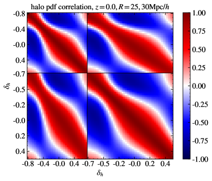
Figure 11: Correlation matrix for the halo PDF in density bins at redshift $z=0$ and radii $R=25,30{\rm Mpc}/h$, extracted from all 15000 realisations of the Quijote fiducial cosmology.

4.4 Fisher Forecast

We quantify the information content of the tracer PDF on key $\Lambda$CDM parameters and the halo bias using the Fisher matrix formalism. Within this formalism we also further validate our theoretical model using the Quijote suite of simulations.

In this section we will introduce the elements that go into the formalism, explain the contents of our data vector, and discuss how combinations of redshifts $z$ and scales $R$ can break degeneracies thus extract the maximum information from the halo density field.

The Fisher matrix is defined by

$$F_{ij}=\sum_{\alpha,\beta}\frac{\partial S_{\alpha}}{\partial\theta_{i}}C_{\alpha\beta}^{-1}\frac{\partial S_{\beta}}{\partial\theta_{j}}$$ (32)

where $S_{i}$ and $\theta_{i}$ are elements of some statistic $\vec{S}$ and some set of parameters $\vec{\theta}$ respectively. $C$ is the data covariance matrix defined by

$$C_{\alpha\beta}=\big{\langle}(S_{\alpha}-\langle S_{\alpha}\rangle)(S_{\beta}-\langle S_{\beta}\rangle)\big{\rangle}.$$ (33)

Here we construct the data vector from the values of the halo one-point PDFs in bins of halo density contrast $\delta_{h}$, combining three different smoothing scales $R$=$20,25,30$Mpc/$h$. We discount the effects of the tails of the PDFs by performing a CDF cut between 0.1,0.05,0.03 for $R=20,25,30$ Mpc/$h$ and 0.9 following the spirit of (Uhlemann et al., 2020). The derivatives $\partial S_{\alpha}/\partial\theta_{i}$ are as discussed in the previous subsection and shown in for $R=25$ Mpc/$h$ in Figure 10. When including the parameter $\beta$, it is treated as separate parameters $\beta_{z}$ for each redshift in the derivatives. The covariance matrix of the halo PDF is the same as previously discussed in Section 4.3. For the Fisher analysis we use a covariance computed from all $N_{\mathrm{sim}}=15,000$ realisations of the Quijote fiducial cosmology. When the covariance matrix is inverted, noise present in the estimation of $C$ will lead to bias in the elements of $C^{-1}$. To correct for this we multiply $C^{-1}$ with the Kaufman-Hartlap factor (Kaufman, 1967; Hartlap et al., 2007) defined by

$$h=\frac{N_{\mathrm{sim}}-2-N_{S}}{N_{\mathrm{sim}}-1}$$ (34)

where $N_{S}$ is the length of the data vector. Since $N_{\mathrm{sim}}=15,000$ is much larger than $N_{S}$ (between 47 and 85 for the PDFs at different redshifts), this factor is always close to unity. We assume no correlation between the density fields at different redshifts, so the Fisher matrices from the three redshifts considered ($z=0.0,0.5,1.0$) can simply be linearly combined. Once the Fisher matrix is known, the marginalised error on the parameter $\theta_{i}$ is given by

$$\delta(\theta_{i})\geq\sqrt{(F)^{-1}_{ii}}.$$ (35)

4.4.1 Validation of tracer PDF constraining power

Before we proceed to making forecasts for the constraining power of the tracer PDF in comparison to the power spectrum, we perform several validations of our theoretical model. When keeping the tracer bias and number density fixed across cosmologies, the matter and tracer PDFs carry a comparable or lower amount of cosmological information as we show in Figure 13. This is expected as for the simple case of linear Eulerian bias and no shot noise there is a simple one-to-one relation between the matter and halo PDFs $\mathcal{P}_{h}(\delta_{h})\simeq\mathcal{P}_{m}(\delta_{m})d\delta_{m}/d\delta_{h}=\mathcal{P}_{m}(\delta_{m}=\delta_{h}/b_{1})/b_{1}$. This is focused on a single redshift $z=0$ and two scales $R=25,30$Mpc$/h$, where we have validated matter (orange solid), halo (blue dashed) and galaxy PDF (green dot-dashed) predictions. The presence of shot noise can lead to a loss of information through the convolution in equation (16), so it is expected that the tracer PDF constraints are weakened with decreasing number density from the halos to the galaxies.

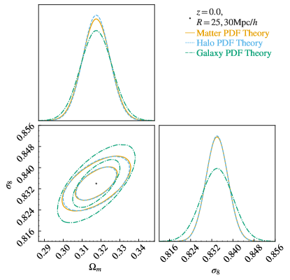
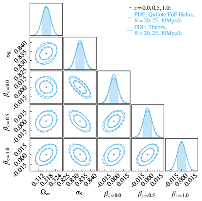
Figure 12: Constraints from theory matter PDFs (orange, solid lines), halo PDFs (blue, dashed lines) and galaxy PDFs (green, dot-dashed) at redshift $z=0.0$ and radii $R=25,30$Mpc/$h$. Halo and galaxy bias theory using Gaussian Lagrangian bias and quadratic shot noise fits from the fiducial cosmology. All other parameters, including bias, are fixed.

Figure 13: Comparison of halo PDF constraints from Quijote (solid, thinner lines) and from theory (dashed, thicker) using Gaussian bias and quadratic shot noise parameters from fits for the fiducial cosmology.

When considering a single redshift but extending the parameter space by one tracer selection parameter $\beta$, the agreement of the Fisher forecasts for theoretical and simulated tracer PDFs is not very good. This can be attributed to the similarity between derivatives w.r.t. the cosmological parameters and the combined bias and stochasticity parameter $\beta$ paired with small residuals in the derivatives. For the galaxies there is a striking similarity between $\sigma_{8}$ and $\beta$ derivatives. For the halos, there is more similarity between the shape of the $\Omega_{m}$ and $\beta$ PDF derivatives. In the more realistic case of combining several redshifts the degeneracy between the cosmological and the combined bias and stochasticity parameter $\beta$ is lifted, such that parameter constraints will become more robust against residual modelling uncertainty.

In Figure 13 we show a comparison of the Fisher forecast for the theoretically predicted and the simulated derivatives finding excellent agreement of the two approaches even after marginalising over one bias parameter $\beta$ per redshift. This reassures us that it is safe to use the theoretical predictions to further explore degeneracy breaking brought about by combining the tracer PDF at different redshifts and adding in the tracer power spectrum, for which we discuss results separately in Appendix B.4.

4.4.2 Degeneracy breaking with different redshifts

Having validated our theoretical models for the tracer PDF and power spectrum, we proceed to forecast parameter constraints at fixed number density to avoid degeneracy breaking arising from different levels of shot noise across the cosmologies. For an initial assessment we consider only one combined tracer bias and stochasticity parameter for both the halo PDFs and the power spectrum.

The upper panel of Figure 14 shows the Fisher forecast for the $\Lambda$CDM parameters $\{\Omega_{m},\sigma_{8}\}$ using data vectors constructed from the theoretical PDFs in $\delta_{h}$ bins with radii $R=20,25,30$ Mpc/$h$ with the bias fixed. Constraints are shown for each redshift $z=0.0,0.5,1.0$ individually in different line style and colour, and then combined in black via a linear combination of the Fisher matrices as appropriate for independent probes. The lower panel also includes a bias parameter $\beta_{z}$ for each redshift. The constraints from these are naturally not combined since these are different parameters.

We can see that the PDFs at different redshifts can break degeneracies present at individual redshifts. As one can see in Figure 10, the PDF derivatives with respect to $\Omega_{m}$ and $\sigma_{8}$ have similar but opposite profiles. This tells us that raising $\Omega_{m}$ and lowering $\sigma_{8}$ have similar effects, which leads to the diagonal alignment of the contours in the upper panel of Figure 14 with the different slopes set by the different amplitude ratios between the two parameter derivatives. This correlation is strongest at $z=1.0$, where as explained for the derivatives above, the response of the PDF to a change in both $\Omega_{m}$ and $\sigma_{8}$ is close to that of rescaling the non-linear variance. On the other hand, at lower redshift the skewness change induced by $\Omega_{m}$ makes the effect of the two parameters more distinguishable. This accounts for the rotation of the ellipses as $z$ decreases.

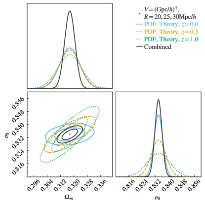
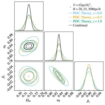
Figure 14: (Upper panel) Fisher forecast for $\{\Omega_{m},\sigma_{8}\}$ for the theory halo PDF at smoothing scales $R=20,25,30{\rm Mpc}/h$ and redshifts $z=0.0,0.5,1.0$ separately and then combined with fixed bias. (Lower panel) also includes the individual bias parameters $\beta_{z}$ for each redshift. Theory PDFs use the Gaussian Lagrangian bias fits and quadratic shot noise fits for the fiducial cosmology.

Figure 15 shows the equivalent plots for the halo power spectrum theory. We see in the upper plot that the $\Omega_{m}$-$\sigma_{8}$ contours have different orientations at different redshifts. As explained in Appendix Section B.4, $\Omega_{m}$ and $\sigma_{8}$ affect the amplitude of the halo power spectrum in opposite ways, but can be distinguished by the Baryon Acoustic Oscillation signature seen in the $\Omega_{m}$ derivative. Furthermore, as in the halo PDF case, the sensitivity of $\Omega_{m}$ to the growth rate accounts for the twisting of the contour orientations across redshift. The power spectrum constraints are less affected by shot noise which lowers the constraining power of the PDF at increasing redshift. The lower panel shows the significant impact of marginalising over the bias which flips the $\sigma_{8}$-$\Omega_{m}$ contour and significantly widens constraints. This is because the profiles of the $\sigma_{8}$ and $\beta$ derivatives seen in Figure 23 are very similar, since these both affect the amplitude in similar ways. On the other hand, $\beta$ and $\Omega_{m}$ affect the amplitude in opposite ways. This accounts for the diagonal contours of different orientation seen in the $\beta_{z}$-$\Omega_{m}$ and $\beta_{z}$-$\sigma_{8}$ panels. When marginalised over the bias parameter $\beta$ the $\sigma_{8}$-$\Omega_{m}$ contours are very similarly diagonally orientated, as the affects can no longer be well distinguished. This can be understood by the similar $\sigma_{8}$ and $\beta$ derivative profiles leading to the remaining part of the $\sigma_{8}$ derivative becoming less distinguishable from $\Omega_{m}$.

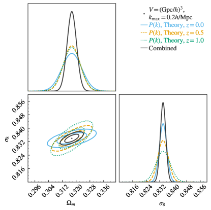
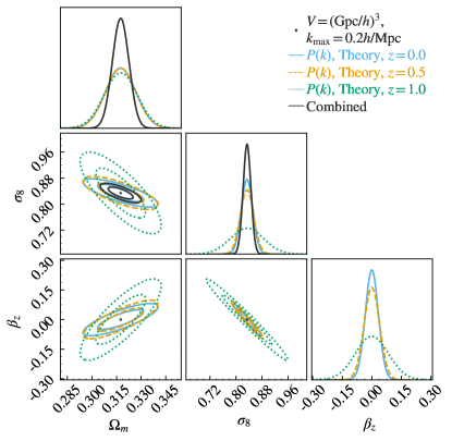
Figure 15: Fisher forecast for $\{\Omega_{m},\sigma_{8}\}$ for the theory halo power spectra at redshifts $z=0.0,0.5,1.0$ separately and then combined. Upper panel with fixed bias, and the lower panel shows also the contours from the individual bias parameters $\beta_{z}$.

4.4.3 Complementarity of tracer PDF and power spectrum

The halo PDF is expected to be complementary to the halo power spectrum as it extracts additional non-Gaussian information encoded in the shape around its peak. To assess the constraining power more quantitatively, we look at Fisher forecasts for the two probes individually and their combination.

As seen in the upper panels of Figures 14 and 15, at fixed bias the halo power spectrum outperforms the PDF. When the cosmology is fixed the constraints on the bias parameters from both probes are very similar and hence not shown separately. As seen in the lower panels of Figures 14 and 15, when jointly constraining cosmology and bias the PDF outperforms the power spectrum. While the $\sigma_{8}$-$\beta$ contours are similarly aligned for PDF and power spectrum, the PDF constraints are much tighter. This demonstrates that the additional non-Gaussian information captured in the PDF can break the degeneracy between $\sigma_{8}$ and bias that is present in the variances and correlation function. When using the PDF, combining different scales effectively captures some compressed information from the power spectrum, namely the variances at the different scales, which is augmented by the non-Gaussian shape around the peak.

Covariance between probes & super-sample covariance

For the combined constraints of the tracer PDFs and the power spectrum we take their full cross-correlation matrix into account, an example of which is shown in Figure 16 for halos at a single redshift, with the PDF at a single scale and the power spectrum. If we focus on mildly nonlinear scales, the tracer power spectrum correlation-matrix is diagonal. The cross-correlation between the PDF and the power spectrum stems from the correlation of the PDF variance with the amplitude of the power spectrum. The band-like structure is caused by the broadness of the smoothing kernel covering all mildly nonlinear $k$-scales shown.

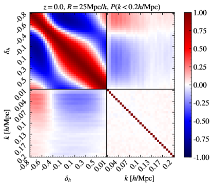
Figure 16: Cross correlation matrix of halo PDF at smoothing scale $R=25{\rm Mpc}/h$ and halo power spectrum at redshift $z=0$.

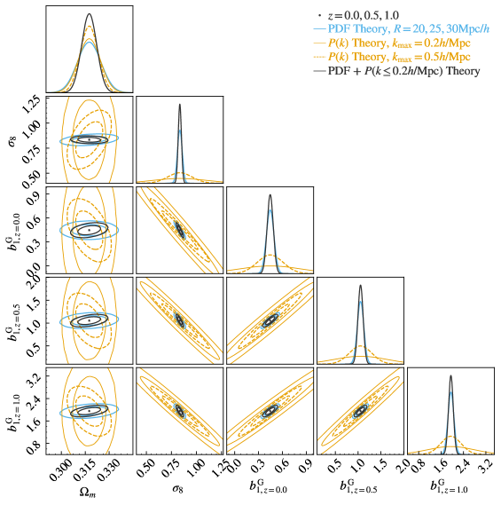
Figure 17: Comparison of constraints from halo PDF theory (blue lines) using fiducial renormalised Gaussian Lagrangian bias fits for all cosmologies and halo power spectra from theory (orange) and their combination (black), shown for the cosmological parameters $\{\Omega_{m},\sigma_{8}\}$ and 1 bias parameter $b^{\mathrm{G}}_{1}=b^{\mathrm{G}}_{1}-1$ for each redshift. Constraints are marginalised over all other bias and shot noise parameters. Results for the halo power spectrum at different $k_{\rm max}$ (orange solid, dashed) illustrate that only information beyond the mildly nonlinear regime can break the degeneracies present in the perturbative regime.

To estimate the impact of super-sample covariance effect that is driven by the background density, we use the separate-universe style ‘DC’ runs of the Quijote simulation suite emulating a background density contrast $\delta_{b}=\pm 0.035$ through changed cosmological parameters and simulation snapshot times from the separate universe approach (Sirko, 2005). The super-sample covariance between two data vector entries $D_{i}$ and $D_{j}$ can be estimated by

$$\text{cov}^{\rm SSC}_{\rm SU}(D_{i},D_{j})=\sigma_{b}^{2}\frac{\partial D_{i}}{\partial\delta_{b}}\frac{\partial D_{j}}{\partial\delta_{b}},$$ (36)

where $\sigma_{b}^{2}$ is the variance of $\delta_{b}$ (here just $\delta_{b}^{2}$), and the other two terms encode the linear response of the data vector, which can be determined from the simulations using finite differences. We add this super-sample covariance term to the measured covariance for both the PDFs and the power spectra.

Marginalising over bias and shot noise parameters

To perform more realistic forecasts between the halo PDF and power spectrum, we have to consider a larger set of independent tracer bias and stochasticity parameters. We proceed with a forecast that varies two cosmological parameters along with one linear bias parameter per redshift, shared between the PDF $b_{1}^{\rm G}$ and the power spectrum $b_{1}=1+b_{1}^{\rm G}$.

Figure 17 shows the Fisher forecast for the halo PDF and power spectrum from theory for the cosmological parameters $\{\Omega_{m},\sigma_{8}\}$ and one shared linear bias parameter $b_{1,z}^{\rm G}$ for each redshift. The analysis combines redshifts $z=0.0,0.5,1.0$ and for the PDFs the smoothing scales $R=20,25,30$ Mpc/$h$. Those constraints are marginalised over one set of additional bias and shot noise parameters per redshift, $\{b_{2}^{\rm G},\alpha_{0},\alpha_{1},\alpha_{2}\}$ for the PDFs across all three scales, and $\{b_{2,k^{2}},\bar{\alpha}_{0}\}$ for the power spectrum. The contours are shown for the halo PDFs and two sets of contours for the power spectrum with $k_{\mathrm{max}}=0.2,0.5h/$Mpc respectively. We observe that at mildly nonlinear scales, the halo power spectrum suffers from the strong degeneracy between $\sigma_{8}$ and linear bias $b_{1}$ and demonstrate that including more nonlinear information through an increase $k_{\rm max}$ increasingly breaks degeneracies. The combined constraints between the mildly nonlinear halo PDF and power spectrum (with the lower $k_{\mathrm{max}}$) are shown in black. In the three right-hand columns of Figure 17, we see that the halo PDF is much better at constraining the bias parameters and indeed dominates the combined constraints. In order to constrain two bias and three shot-noise parameters for the PDF per redshift, combining different scales is crucial. Additionally, combining different redshifts tightens the cosmological constraints which in turn helps to fix the bias and stochasticity parameters, for both the PDF and the power spectrum.

Including super-sample covariance leads to a mild widening of the contours on both the PDFs and power spectrum. For $\sigma_{8}$ errors increase by 4% and 11% for the halo PDFs and power spectra, respectively. For $\Omega_{m}$ errors increase by 3% and less than 1%. For the three $b^{\mathrm{G}}_{1,z}$ parameters at z=0,0.5,1 the errors widen by {16,25,5}% and {11,5,4}% for the halo PDF and power spectrum, respectively. This is also accompanied by a minor rotation in the degeneracy directions.

5 Conclusions

5.1 Summary

In this paper we have adapted a model of the conditional PDF of tracer counts given matter density (14) (introduced for photometric data in Friedrich et al. (2022)) to a spectroscopic setting. We have shown that a 2-parameter Gaussian Lagrangian bias model recently proposed in Stücker et al. (2024a, b) and a quadratic shot noise model provide accurate parameterisations of its two ingredients for both halos and HOD-populated galaxies. We validated the theoretical predictions against the tracer PDFs for dark matter halos extracted from the Quijote suite of N-body simulations and galaxies from the associated Molino suite. In both cases we find excellent agreement of no more than 2% around the central region of the PDF. We related our conditional PDF parameters to the power spectrum bias and stochasticity parameters. The Eulerian linear bias in the power spectrum and first Gaussian Lagrangian parameter are roughly related by $b_{1}^{\mathrm{E}}\approx 1+b_{1}^{\mathrm{G}}$. The renormalised Gaussian Lagrangian bias model we adopt gives bias parameters that are very close to scale-dependent across different scales. The quadratic shot noise parameters show some scale-dependence, although we found its impact on the tracer PDFs to be mild. The power spectrum shot noise amplitude $\bar{\alpha}_{0}$ is close to the shot noise amplitude obtained from variances that can be linked to the quadratic shot noise model as discussed in Appendix A.2. This is a promising first step towards allowing a joint analysis of the tracer PDF and power spectrum with shared bias and stochasticity parameters.

We validated the response of the halo and galaxy PDF to changes in cosmology (at fixed bias) and tracer selection by comparing parameter derivatives with respect to $\{\Omega_{m},\sigma_{8}\}$ and one effective bias parameter $\beta_{z}$ per redshift in Figure 10. We also validated the constraining power of the theory on the same parameters when combining different redshifts with a Fisher forecast in Figure 13.

After validating the constraining power of the theory, we performed Fisher forecasts at fixed number density with the theoretical model comparing the tracer PDF with the power spectrum. Figure 17 shows the constraints for the parameters {$\Omega_{m},\sigma_{8},b_{1,z}^{\rm G}$} for both halo PDF and power spectrum theory and their combination across three redshifts. In our model, the Eulerian linear bias of the power spectrum is tied to the renormalised Lagrangian Gaussian bias of the PDF as $b_{1}=1+b_{1}^{\rm G}$. The strength of the PDF is disentangling the effect of changing bias to that of changing $\sigma_{8}$. The combined constraints are dominated by the PDF, but tightened by additional degeneracy breaking. While our adopted tracer power spectrum model (combining the halofit matter power spectrum with a linear but scale-dependent bias and a white noise stochasticity) is simplistic, state-of-the-art perturbation-theory based models will likely contain more free parameters.

The spectroscopic one-point tracer PDF is a promising probe of cosmology on mildly non-linear scales and complementary to standard two-point statistics.

5.2 Outlook

In this work we focused on biased tracers in real space. For an application to spectroscopic clustering survey data, we will need to understand their one-point statistics in redshift space. Therefore, future work will need to model the effect of redshift space distortions. Previous work on incorporating the impact of redshift-space distortions through a modification of the matter variance (Repp and Szapudi, 2020) or absorbing it in an effective bias model (Uhlemann et al., 2018) will be useful starting points for this. To extract additional information from redshift space distortions, the concept of a 2D-kNN statistics distinguishing between radial and angular distances (Yuan et al., 2023) could be translated to the PDF by using spheroidal cells.

Here we use simulated covariance matrices for the tracer PDFs and power spectra calculated from a large number of realisations at a fiducial cosmology. Uhlemann et al. (2022) shows that it is possible to predict covariances for the 3D matter PDF from theory, including the predictions for the super-sample covariance. Future work could extend this to tracer PDFs and their cross-correlation with tracer power spectra.

Our tracer PDF is parameterised by two bias parameters $\{b_{1}^{\mathrm{G}},b_{2}^{\mathrm{G}}\}$ and three shot noise parameters $\{\alpha_{0},\alpha_{1},\alpha_{2}\}$ per redshift, where the latter can vary across smoothing scale. Our Fisher analysis only includes one shared linear bias parameter between halo PDFs of all scales and the power spectrum at each redshift, and marginalises over one set of nonlinear bias and stochasticity parameters for the PDFs across three scales and the power spectrum, respectively. Better understanding of effective tracer bias parametrisations (see e.g. Banerjee et al., 2022) and stochasticity parametrisations (including HOD-informed parameter bounds Britt et al., 2024) will be required to leverage the power of theoretical one-point statistic models for jointly constraining cosmology and astrophysical parameters from data.

Data Availability

The data products were extracted with the public code Pylians3 from the publicly available Quijote simulations (Villaescusa-Navarro et al., 2019) and the Molino catalogs (Hahn and Villaescusa-Navarro, 2021). The measured tracer PDFs, conditional moments and power spectra are made available on the Quijote Globus.

Appendix A Tracer-matter connection

A.1 Fine sampling limits for tracer PDFs

In the limit of fine sampling $\bar{N}_{t}\rightarrow\infty$, the conditional PDF (14) and the integral to obtain the tracer count PDF (16) with the matter PDF can be simplified. In the spirit of large-deviations theory, we start by writing the conditional PDF for $N_{t}=\bar{N}_{t}(1+\delta_{t})$ given matter density $\delta_{m}$ in terms of a function that is exponentially decaying with increasing $\bar{N}_{t}$

$$-\frac{\ln\mathcal{P}(N_{t}|\delta_{m})}{\bar{N}_{t}}= \frac{1+b(\delta_{m})}{\alpha(\delta_{m})}-\frac{1+\delta_{t}}{\alpha(\delta_{m})}\ln\left(\frac{\bar{N}_{t}(1+b(\delta_{m}))}{\alpha(\delta_{m})}\right)$$

$$+\frac{1}{\bar{N}_{t}}\ln\Gamma\left(1+\frac{\bar{N}_{t}(1+\delta_{t})}{\alpha(\delta_{m})}\right)$$ (37a)

$$+\frac{\ln\alpha(\delta_{m})}{\bar{N}_{t}}\,.$$

We obtain a rate function (1) from the limit $$\bar{N}_{t}\rightarrow\infty \epsilon=1/\bar{N}_{t}\rightarrow 0$$ (corresponding to a driving parameter )

$$-\lim_{\bar{N}_{t}\rightarrow\infty}\frac{\ln\mathcal{P}(N_{t}|\delta_{m})}{\bar{N}_{t}}:=\psi_{t|m}(\delta_{t};\delta_{m})\,.$$ (37b)

We use Stirling’s formula for large arguments of the Gamma function (reducing to the factorial for integers)

$$\ln\Gamma(1+x)\approx x(\ln x-1)+\ln[(2\pi x)^{1/2}]\,,$$ (37c)

where the second term does not affect the exponential decay, but is relevant for the normalisation. We find

$$\psi_{t|m}(\delta_{m};\delta_{t})=\frac{b(\delta_{m})-\delta_{t}+(1+\delta_{t})\ln\left(\frac{1+\delta_{t}}{1+b(\delta_{m})}\right)}{\alpha(\delta_{m})}\,.$$ (37d)

A.1.1 Fine sampling limit for the conditional tracer PDF

To obtain the fine-sampling limit for the conditional PDF $\mathcal{P}(N_{t}|\delta_{m})$, we can Taylor-expand the function $\psi_{t|m}(\delta_{t};\delta_{m})$ around its minimum at the most likely value $\delta_{t}^{*}$ given $\delta_{m}$. We have that $\psi_{t|m}(\delta_{t}^{*})=0$ for $\delta_{t}^{*}=b(\delta_{m})$. The first derivative w.r.t. to $\delta_{t}$ is

$$\psi_{t|m}^{\prime}(\delta_{t})=\frac{\ln\left(\frac{1+\delta_{t}}{1+b(\delta_{m})}\right)}{\alpha(\delta_{m})}\,,$$ (37e)

and thus zero at $\delta_{t}^{*}$ showing that is is indeed an extremum. The second derivative yields

$$\psi_{t|m}^{\prime\prime}(\delta_{t})=\frac{1}{\alpha(\delta_{m})(1+\delta_{t})}>0\,,$$ (37f)

which shows the extremum is in fact a minimum. With this we can write

$$\psi_{t|m}(\delta_{t})\approx\frac{(\delta_{t}-b(\delta_{m}))^{2}}{2\alpha(\delta_{m})(1+b(\delta_{m}))}\,.$$ (37g)

After having identified the peak of the PDF at $\delta_{t}^{*}=b(\delta_{m})$ in the limit of $\bar{N}_{t}\rightarrow\infty$, we can attempt to restore the normalisation at finite $\bar{N}_{t}$. Considering the last term of the original exponent (37) along with the sub-leading term in the Stirling approximation (37c), we obtain

$$\mathcal{P}(N_{t}|\delta_{m})\approx \left[2\pi N_{t}\alpha(\delta_{m})\right]^{-\frac{1}{2}}\exp\left[-\bar{N}_{t}\psi_{t|m}(\delta_{t})\right]\,,$$

where the exponential is quadratic as given by equation (37g) and $N_{t}=\bar{N}_{t}(1+\delta_{t})$. This shows that the conditional PDF $\mathcal{P}(N_{t}|\delta_{m})$ tends to a Gaussian with mean $\bar{N}_{t}(1+b(\delta_{m}))$ and variance $\alpha(\delta_{m})\bar{N}_{t}(1+b(\delta_{m}))$. We can convert this to the conditional PDF of tracer density contrast

$$\mathcal{P}(\delta_{t}|\delta_{m})\approx \left[2\pi\frac{\alpha(\delta_{m})(1+b(\delta_{m}))}{\bar{N}_{t}}\right]^{-\frac{1}{2}}$$ (37h)

$$\times\exp\left[-\bar{N}_{t}\frac{(\delta_{t}-b(\delta_{m}))^{2}}{2\alpha(\delta_{m})(1+b(\delta_{m}))}\right]\,,$$

which is a Gaussian with mean $b(\delta_{m})$ and variance $\alpha(\delta_{m})(1+b(\delta_{m}))/\bar{N}_{t}$.

A.1.2 Fine sampling limit for the tracer PDF

Let us now use similar arguments to simplify the tracer PDF (16) given as $\delta_{m}$-integral over the product of the conditional PDF (14) and the matter PDF. For the $\delta_{m}$ integral in equation (16), $\delta_{t}$ can be considered a constant. Evidently, $\psi_{t|m}(\delta_{m}^{*})=0$ for $\delta_{m}^{*}$ such that $\delta_{t}=b(\delta_{m}^{*}).$ Let us consider the first derivative of $\psi_{t|m}(\delta_{m};\delta_{t})$ w.r.t $\delta_{m}$

$$\psi_{t|m}^{\prime}(\delta_{m})=\frac{b^{\prime}(\delta_{m})}{\alpha(\delta_{m})}\left[1-\frac{1+\delta_{t}}{1+b(\delta_{m})}\right]-\frac{\alpha^{\prime}(\delta_{m})}{\alpha(\delta_{m})}\psi_{t|m}(\delta_{m})\,,$$ (38)

which also vanishes at $\delta_{m}^{*}$ making this an extremum. The second derivative is

$$\psi_{t|m}^{\prime\prime}(\delta_{m}) =\frac{b^{\prime}(\delta_{m})}{\alpha(\delta_{m})}\frac{b^{\prime}(\delta_{m})(1+\delta_{t})}{(1+b(\delta_{m}))^{2}}$$ (39)

$$+\left(\frac{b^{\prime}(\delta_{m})}{\alpha(\delta_{m})}\right)^{\prime}\left[\frac{b(\delta_{m})-\delta_{t}}{1+b(\delta_{m})}\right]$$

$$-\left(\frac{\alpha^{\prime}(\delta_{m})}{\alpha(\delta_{m})}\right)^{\prime}\psi_{t|m}(\delta_{m})-\frac{\alpha^{\prime}(\delta_{m})}{\alpha(\delta_{m})}\psi_{t|m}^{\prime}(\delta_{m})\,.$$

At the extremum $\delta_{m}^{*}$ where $\delta_{t}=b(\delta_{m}^{*})$ only the first term remains

$$\psi_{t|m}^{\prime\prime}(\delta_{m}^{*})=\frac{b^{\prime}(\delta_{m}^{*})^{2}(1+\delta_{t})}{\alpha(\delta_{m}^{*})[1+b(\delta_{m}^{*})]^{2}}=\frac{b^{\prime}(\delta_{m}^{*})^{2}}{\alpha(\delta_{m}^{*})(1+\delta_{t})}>0\,,$$ (40)

which shows that $\delta_{m}^{*}$ is a minimum. This leads to the conditional PDF (14) resembling a Gaussian function around the saddle point $\delta_{m}^{*}(\delta_{t})$

$$\exp\left[-\bar{N}_{t}\psi_{t|m}(\delta_{t};\delta_{m})\right] \propto\exp\left[-\frac{[\delta_{m}-\delta_{m}^{*}(\delta_{t})]^{2}}{2\sigma_{*}^{2}(\delta_{m}^{*}(\delta_{t}))}\right]$$ (41)

$$\sigma_{*}^{2}(\delta_{m}^{*}(\delta_{t})) =\frac{\alpha(\delta_{m}^{*}(\delta_{t}))(1+\delta_{t})}{\bar{N}_{t}b^{\prime}(\delta_{m}^{*}(\delta_{t}))^{2}}\,.$$ (42)

As before, the normalisation is $[2\pi N_{t}\alpha(\delta_{m}^{*}(\delta_{t}))]^{-1/2}$ with $N_{t}=\bar{N}_{t}(1+\delta_{t})$. When converting the PDF ot the tracer count $\mathcal{P}_{t}(N_{t})$ to the PDF of the tracer density contrast $\mathcal{P}_{t}(\delta_{t})$, we obtain an extra factor of $\bar{N}_{t}$ such that the prefactor changes to $[2\pi\alpha(\delta_{m}^{*}(\delta_{t}))(1+\delta_{t})/\bar{N}_{t}]^{-1/2}$. This can be rewritten as $(2\pi\sigma_{*}^{2})^{-1/2}/b^{\prime}(\delta_{m}^{*}(\delta_{t}))$. The integral becomes a convolution of the matter PDF with a zero-mean Gaussian of variance $\sigma_{*}^{2}(\delta_{t})$ such that

$$\mathcal{P}_{t}(\delta_{t})\approx\frac{1}{b^{\prime}(\delta_{m}^{*}(\delta_{t}))}\Big{(}\mathcal{P}_{G}\!\left(\sigma_{*}^{2}(\delta_{t})\right)\!\,*\mathcal{P}_{m}\Big{)}\left(\delta_{m}^{*}(\delta_{t})\right)\,.$$ (43)

We can see that in the asymptotic limit of $\bar{N}_{t}\rightarrow\infty$, the Gaussian becomes a delta function and we obtain

$$\mathcal{P}_{t}(\delta_{t})\stackrel{{\scriptstyle\bar{N}_{t}\rightarrow\infty}}{{\longrightarrow}}\frac{1}{b^{\prime}(\delta_{m}^{*}(\delta_{t}))}\mathcal{P}_{m}\left(\delta_{m}^{*}(\delta_{t})\right)\,,$$ (44)

where we can replace $\delta_{m}^{*}=b^{-1}(\delta_{t})$. In this model, the asymptotic limit thus corresponds to a deterministic bias where $\mathcal{P}_{t}(\delta_{t})=\mathcal{P}_{m}(\delta_{m}(\delta_{t}))d\delta_{m}/d\delta_{t}$. Note that even if the PDF of $\delta_{m}^{*}$ was Gaussian, a nonlinear bias $\delta_{t}=b(\delta_{m}^{*})$ would imply a non-Gaussian PDF for $\delta_{t}$.

If the matter PDF was a zero-mean Gaussian with variance $\sigma_{m}^{2}$, then the convolution would be another Gaussian function with an increased density-dependent variance $\sigma^{2}(\delta_{t})=\sigma_{m}^{2}+\sigma_{*}^{2}(\delta_{t})$. Thus, the exponent of the PDF for $\delta^{*}_{m}(\delta_{t})$ would agree with the one of matter PDF evaluated at $\delta_{m}(\delta_{t})=\delta_{m}^{*}(\delta_{t})/\sqrt{1+\sigma_{*}^{2}(\delta_{t})/\sigma_{m}^{2}}$. Note that even if the PDF of $\delta_{m}^{*}$ was Gaussian and the bias was linear, the $\delta_{t}$-dependence of the variance would imply a non-Gaussian PDF for $\delta_{t}$.

A.2 Tracer-matter spectra and covariances

A.2.1 Tracer-matter cross and auto spectra

Here we further connect the conditional mean bias and stochasticity models presented in Sections 3.2 and 3.3 to the bias and stochasticity in the power spectrum used in Section 3.5. Let us briefly summarise how a Eulerian quadratic bias model manifests in the tracer cross and auto power spectra. We start with the noise-free tracer density

$$\tilde{\delta}_{t}(\vec{x})= b_{1}\delta_{m}(\vec{x})+\frac{b_{2}}{2}\left(\delta_{m}(\vec{x})^{2}-\langle\delta_{m}(\vec{x})^{2}\rangle\right)$$ (45a)

$$+\frac{b_{s^{2}}}{2}\left(s_{ij}(\vec{x})^{2}-\langle s_{ij}(\vec{x})^{2}\rangle\right)\,,$$

where $$b_{s^{2}} s_{ij}=(\partial_{i}\partial_{j}/\partial^{2}-\delta_{ij}/3)\delta_{m}(\vec{x})$$ describes the non-local bias associated with the tidal shear . In Fourier space this translates to

$$\tilde{\delta}_{t}(\vec{k})= b_{1}\delta_{m}(\vec{k})+\frac{b_{2}}{2}\overbrace{\int\!d^{3}q\,\delta_{m}(\vec{k}-\vec{q})\delta_{m}(\vec{q})}^{(\delta_{m}*\delta_{m})(\vec{k})}$$ (45b)

$$+\frac{b_{s^{2}}}{2}\underbrace{\int\!d^{3}q\,\delta_{m}(\vec{k}-\vec{q})\delta_{m}(\vec{q})S_{2}(\vec{q},\vec{k}-\vec{q})}_{(s_{ij}*s_{ij})(\vec{k})}\,,$$

where $$S_{2}(\vec{q_{1}},\vec{q_{2}})=\vec{q_{1}}\cdot\vec{q_{2}}/(q_{1}^{2}q_{2}^{2})-1/3 \delta \langle\cdot\rangle$$ and we omitted the -function terms that arise from the subtraction of the constant expectation values . With this we obtain the cross power spectrum

$$P_{tm}(k) =\langle\delta_{t}(\vec{k})\delta_{m}(-\vec{k})\rangle$$

$$=b_{1}P_{m}(k)+\frac{b_{2}}{2}\int\!d^{3}qB_{m}(\vec{q},\vec{k}-\vec{q},-\vec{k})$$

$$+\frac{b_{s^{2}}}{2}\int\!d^{3}qS_{2}(\vec{q},\vec{k}-\vec{q})B_{m}(\vec{q},\vec{k}-\vec{q},-\vec{k})\,,$$ (45c)

which depends on the matter power spectrum $$P_{m} B_{m}$$ and two integrals over the bispectrum , one of which is the skew-spectrum. The bias function (26) is then obtained as

$$b(k)=\frac{P_{tm}(k)}{P_{m}(k)} =b_{1}+\frac{b_{2}}{2}\frac{\int\!d^{3}qB_{m}(\vec{q},\vec{k}-\vec{q},-\vec{k})}{P_{m}(k)}$$ (45d)

$$+\frac{b_{s^{2}}}{2}\frac{\int\!d^{3}qS_{2}(\vec{q},\vec{k}-\vec{q})B_{m}(\vec{q},\vec{k}-\vec{q},-\vec{k})}{P_{m}(k)}\,,$$

where the quadratic terms term would typically be evaluated within perturbation theory and lead to either constant terms that combine with $$b_{1} k^{2}$$ or a leading-order scale dependence of .

For the case of just local bias (thus neglecting the tidal bias term $b_{s^{2}}$), the tracer auto power spectrum is obtained as

$$P_{t}(k) =\langle\delta_{t}(\vec{k})\delta_{t}(-\vec{k})\rangle$$

$$=b_{1}^{2}P_{m}(k)+b_{1}b_{2}\langle(\delta_{m}*\delta_{m})(\vec{k})\delta_{m}(-\vec{k})\rangle$$ (46a)

$$+\frac{b_{2}^{2}}{4}\langle(\delta_{m}*\delta_{m})(\vec{k})(\delta_{m}*\delta_{m})(\vec{-k})\rangle+P_{\epsilon}(k)$$

$$=b_{1}^{2}P_{m}(k)+b_{1}b_{2}\int\!d^{3}qB_{m}(\vec{q},\vec{k}-\vec{q},-\vec{k})$$ (46b)

$$+\frac{b_{2}^{2}}{4}\!\!\int\!\!\!\!\int\!\!d^{3}q_{1}d^{3}q_{2}T_{m}(\vec{q_{1}},\vec{q_{2}},\vec{k}-\vec{q_{1}},-\vec{k}-\vec{q_{2}})+P_{\epsilon}(k)\,,$$

which depends on the matter power spectrum, the skew-spectrum and an integrated version of the trispectrum $$T_{m} P_{\epsilon}(k)=\langle\epsilon(\vec{k})\epsilon(-\vec{k})\rangle S_{2}$$ and the shot noise power spectrum . The tidal bias terms will involve similar integrals with additional weightings with one kernel for the bispectrum and two for the trispectrum term. The shot noise defined in (27) would then be given by

$$\frac{\alpha(k)}{\bar{n}} =\frac{b_{2}^{2}}{4}\Bigg{[}\!\!\int\!\!\!\!\int\!\!d^{3}q_{1}d^{3}q_{2}T_{m}(\vec{q_{1}},\vec{q_{2}},\vec{k}-\vec{q_{1}},-\vec{k}-\vec{q_{2}})$$

$$\qquad-\frac{\left(\int\!d^{3}qB_{m}(\vec{q},\vec{k}-\vec{q},-\vec{k})\right)^{2}}{P_{m}(k)}\Bigg{]}+P_{\epsilon}(k)\,,$$ (46c)

where the terms including the trispectrum and square of the bispectrum are of higher perturbative order. As expected, nonlinear bias does contribute to the shot noise defined relative to the linear bias. This is in contrast to the shot noise defined based on the conditional variance (23) which would vanish for any nonlinear but still deterministic local bias.

A.2.2 Tracer-matter covariances from bias and stochasticity

Let us connect the conditional mean bias presented in Section 3 to the cross-covariance between tracer and halo densities. We can obtain the covariance between tracer and matter densities from the joint PDF (13)

$$\sigma_{tm}^{2} =\langle\delta_{t}\delta_{m}\rangle=\int d\delta_{m}\!\!\int\!d\delta_{t}\,\delta_{t}\delta_{m}\mathcal{P}(\delta_{t}|\delta_{m})\mathcal{P}_{m}(\delta_{m})$$

$$=\int\langle\delta_{t}|\delta_{m}\rangle\delta_{m}\mathcal{P}(\delta_{m})d\delta_{m}=\langle b(\delta_{m})\delta_{m}\rangle\,.$$ (47a)

For a quadratic Eulerian bias (17), we have that

$$\sigma_{tm}^{2}=b_{1}\sigma_{m}^{2}+\frac{b_{2}}{2}\langle\delta_{m}^{3}\rangle\,,$$ (47b)

where for brevity we wrote $$b_{n} b_{n}^{\rm E}$$ instead of for the Eulerian bias parameters. This closely resembles the result for the tracer-matter cross power spectrum (45). For a Gaussian field, the quadratic bias term would not affect the tracer-matter covariance. In analogy to the power spectrum bias (26), we can define a bias from the ratio of the tracer-matter covariance and matter variance

$$b_{\times,\sigma^{2}} =\frac{\sigma_{tm}^{2}}{\sigma_{m}^{2}}=\frac{\langle b(\delta_{m})\delta_{m}\rangle}{\langle\delta_{m}^{2}\rangle}$$ (47c)

$$=b_{1}+\frac{b_{2}}{2}\frac{\langle\delta_{m}^{3}\rangle}{\sigma_{m}^{2}}=b_{1}+\frac{b_{2}}{2}S_{3}\sigma_{m}^{2}\,.$$ (47d)

The presence of the second term nicely illustrates how the non-Gaussianity of the late-time matter field increases the relevance of the nonlinearity in the bias. To obtain the variance of the tracer density $\sigma_{t}^{2}$, we will additionally require a description of shot noise.

After determining how the conditional mean bias sets the covariance between tracer and matter densities (47a), let us determine how it propagates into the variance of tracer densities together with the shot noise.

$$\sigma_{t}^{2} =\langle\delta_{t}^{2}\rangle=\int d\delta_{m}\!\!\int\!d\delta_{t}\,\delta_{t}^{2}\mathcal{P}(\delta_{t}|\delta_{m})\mathcal{P}_{m}(\delta_{m})$$

$$=\int\overbrace{\left(\langle\delta_{t}|\delta_{m}\rangle^{2}+\langle\delta_{t}^{2}|\delta_{m}\rangle_{c}\right)}^{\langle\delta_{t}^{2}|\delta_{m}\rangle}\mathcal{P}(\delta_{m})d\delta_{m}$$ (48)

$$=\int\left(\langle\delta_{t}|\delta_{m}\rangle^{2}+\frac{\alpha(\delta_{m})(1+\langle\delta_{t}|\delta_{m}\rangle)}{\bar{N}_{t}}\right)\mathcal{P}(\delta_{m})d\delta_{m}$$

Let us split the result into to terms. The first term is the variance for a shot-noise free tracer density $$\tilde{\delta}_{t}$$

$$\tilde{\sigma}_{t}^{2} =\langle\tilde{\delta}_{t}^{2}\rangle=\langle b^{2}(\delta_{m})\rangle)\,.$$ (49a)

This can be expanded for a quadratic Eulerian bias (17)

$$\tilde{\sigma}_{t}^{2} =b_{1}^{2}\sigma_{m}^{2}+b_{1}b_{2}\langle\delta_{m}^{3}\rangle+\frac{b_{2}^{2}}{4}\left(\langle\delta_{m}^{4}\rangle-\sigma_{m}^{4}\right)\,.$$ (49b)

Even for a Gaussian field, the quadratic bias affects the tracer variance while the tracer-matter covariance was unaffected, similarly as for the tracer power spectra.

The second term includes the shot noise

$$\sigma_{\rm\alpha}^{2} =\sigma_{t}^{2}-\tilde{\sigma}_{t}^{2}=\frac{\langle\alpha(\delta_{m})\rangle+\langle\alpha(\delta_{m})b(\delta_{m})\rangle}{\bar{N}_{t}}\,,$$ (50a)

and can be expanded for a quadratic model (24)

$$\sigma_{\rm\alpha}^{2} =\frac{\alpha_{0}+(\alpha_{0}b_{1}+\alpha_{1})\langle\delta_{m}\rangle+(\alpha_{2}+\alpha_{1}b_{1})\langle\delta_{m}^{2}\rangle}{\bar{N}_{t}}$$

$$+\frac{(\alpha_{1}\frac{b_{2}}{2}+\alpha_{2}b_{1})\langle\delta_{m}^{3}\rangle+\alpha_{2}\frac{b_{2}}{2}\langle\delta_{m}^{2}(\delta_{m}^{2}-\sigma_{m}^{2})\rangle}{\bar{N}_{t}}$$

$$=\frac{\alpha_{0}+(\alpha_{1}b_{1}+\alpha_{2})\sigma_{m}^{2}}{\bar{N}_{t}}$$ (50b)

$$+\frac{(\alpha_{1}\frac{b_{2}}{2}+\alpha_{2}b_{1})S_{3}\sigma_{m}^{4}+\alpha_{2}\frac{b_{2}}{2}(2\sigma_{m}^{4}+S_{4}\sigma_{m}^{6})}{\bar{N}_{t}}\,.$$

For linear bias and linear shot noise only the first line remains, which still present an interesting coupling of the linear bias and shot noise parameters at leading order in the dark matter variance $$\sigma_{m}^{2}$$.

In analogy to the power spectrum shot noise with respect to linear bias (27), one can define a shot noise parameter obtained from the covariance and variances of tracer and matter densities

$$\alpha_{\sigma^{2}}=\bar{N}_{t}\left(\sigma_{t}^{2}-\frac{\sigma_{tm}^{4}}{\sigma_{m}^{2}}\right)=\bar{N}_{t}\left(\sigma_{t}^{2}-b_{\times,\sigma^{2}}^{2}\sigma_{m}^{2}\right)\,,$$ (51a)

for which we list measured values for the fiducial cosmology in Table 6. For quadratic models for Eulerian bias and shot noise, the stochasticity parameter $$\alpha_{\sigma^{2}}$$ is obtained from inserting equations (47d) and (A.2.2)

$$\frac{\alpha_{\sigma^{2}}}{\bar{N}_{t}} =\sigma_{\alpha}^{2}+\frac{b_{2}^{2}}{4}\underbrace{\left(\langle\delta_{m}^{4}\rangle-\sigma_{m}^{4}-\frac{\langle\delta_{m}^{3}\rangle^{2}}{\sigma_{m}^{2}}\right)}_{\sigma_{m}^{4}[2+(S_{4}-S_{3}^{2})\sigma_{m}^{2}]}\,.$$ (51b)

We can see that the size of the $b_{2}^{2}$ term is controlled by the square of the variance $\sigma_{m}^{4}$ and thus higher order, similarly as for the power spectrum (46). In addition, we have several coupling terms between stochasticity and bias parameters $\alpha_{k}b_{n-k}$ scaling as $\sigma_{m}^{4}$.

We can also obtain an associated linear correlation coefficient

$$r=\frac{\sigma_{tm}^{2}}{\sqrt{\sigma_{t}^{2}\sigma_{m}^{2}}}=\left(1+\frac{\alpha_{\sigma^{2}}}{\bar{N}_{t}b_{\times,\sigma^{2}}^{2}\sigma_{m}^{2}}\right)^{-1/2}\,,$$ (52)

which is between $0.9$ and $0.95$ for our halo samples across different scales and redshifts.

z	$\bar{\alpha}_{0}$	$\alpha_{\sigma^{2}}(R$ [Mpc$/h$])
		$R=30$	$R=25$	$R=20$
0.0	0.83	0.85	0.82	0.80
0.5	0.67	0.65	0.64	0.63
1.0	0.75	0.73	0.72	0.71

Table 6: Values of halo stochasticity parameters fitted from the power spectrum (27) and measured (co)variances (51) for the fiducial cosmology.

A.2.3 Higher-order tracer moments

We can also compute higher-order moments for the tracer distribution, for example the third moment

$$\langle\delta_{t}^{3}\rangle=\int d\delta_{m}\!\!\int\!d\delta_{t}\,\delta_{t}^{3}\mathcal{P}(\delta_{t}|\delta_{m})\mathcal{P}_{m}(\delta_{m})$$ (53a)

$$=\int\overbrace{\left(\langle\delta_{t}|\delta_{m}\rangle^{3}+3\langle\delta_{t}^{2}|\delta_{m}\rangle_{c}\langle\delta_{t}|\delta_{m}\rangle+\langle\delta_{t}^{3}|\delta_{m}\rangle_{c}\right)}^{\langle\delta_{t}^{3}|\delta_{m}\rangle}\mathcal{P}(\delta_{m})d\delta_{m}\,,$$

Again, we will split it into a shot-noise free term

$$\langle\tilde{\delta}_{t}^{3}\rangle =\langle b(\delta_{m})^{3}\rangle\,,$$ (53b)

and a shot noise contribution

$$\langle\delta_{t}^{3}\rangle-\langle\tilde{\delta}_{t}^{3}\rangle =3\frac{\langle\alpha(\delta_{m})b(\delta_{m})\rangle+\langle\alpha(\delta_{m})b(\delta_{m})^{2}\rangle}{\bar{N}_{t}}$$ (53c)

$$\quad+\frac{\langle\alpha(\delta_{m})^{2}\rangle+\langle\alpha(\delta_{m})^{2}b(\delta_{m})\rangle}{\bar{N}_{t}^{2}}\,,$$

where we used that $$\langle N_{t}^{3}|\delta_{m}\rangle_{c}=\alpha(\delta_{m})^{2}\bar{N}_{t}(\delta_{m})$$. We now consider the contributions from a quadratic Eulerian bias

$$\langle\tilde{\delta}_{t}^{3}\rangle =b_{1}^{3}\langle\delta_{m}^{3}\rangle+\frac{3b_{1}b_{2}}{2}\left(b_{1}\langle\delta_{m}^{4}\rangle+\frac{b_{2}}{2}\langle\delta_{m}^{5}\rangle\right)+\frac{b_{2}^{3}}{8}\langle\delta_{m}^{6}\rangle\,,$$ (53d)

and the coupling of linear stochasticity and bias

$$\langle\delta_{t}^{3}\rangle-\langle\tilde{\delta}_{t}^{3}\rangle \stackrel{{\scriptstyle\text{lin}}}{{\approx}}\,3\frac{(\alpha_{1}b_{1}+\alpha_{0}b_{1}^{2})\sigma_{m}^{2}+\alpha_{1}b_{1}^{2}\langle\delta_{m}^{3}\rangle}{\bar{N}_{t}}$$ (53e)

$$\quad+\frac{\alpha_{0}^{2}+\alpha_{1}(\alpha_{1}+2\alpha_{0}b_{1})\sigma_{m}^{2}+\alpha_{1}^{2}b_{1}\langle\delta_{m}^{3}\rangle}{\bar{N}_{t}^{2}}\,.$$

Those results could be used to approximate the tracer PDF by a shifted lognormal distribution by imposing the right variance and skewness through the lognormal shift parameter.

Appendix B Additional Details & Validations

B.1 Matter PDF derivatives

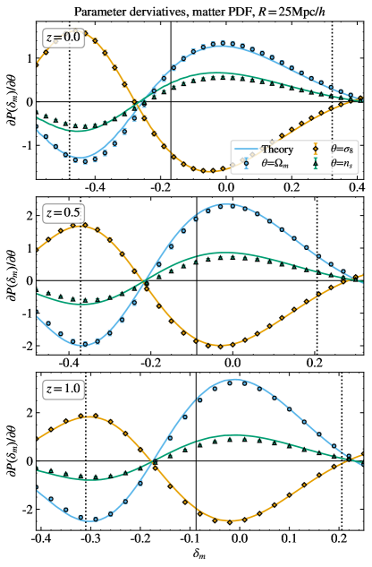
Figure 18: Derivatives of the matter PDF with respect to cosmological parameters. Theory using re-scaled non-linear matter variance for each cosmology.

Figure 18 shows a comparison of the simulated and predicted derivatives of the matter PDFs when changing cosmological parameters. The matter PDFs for all cosmologies are predicted using a non-linear matter variance $\sigma_{\mathrm{NL}}^{2}$ rescaled via the ratio between that for the fiducial cosmology predicted in CosMomentum and measured from Quijote . We see a good agreement, in line with previous results using a saddle-point approximation for the log-density (Uhlemann et al., 2020).

B.2 Tracer PDF residuals

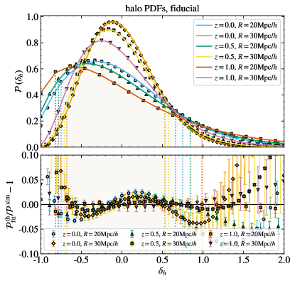
Figure 19: Halo PDF as measured from Quijote (data points) and predicted from CosMomentum with renormalised Gaussian Lagrangian bias and quadratic shot noise fits.

Figure 19 shows a model validation for the fiducial halo PDFs across different scales and redshifts. The theory PDFs are predicted using the fitted renormalised Gaussian Lagrangian parameters and quadratic shot noise parameters, both fitted over smoothing scales $R=20,25,30$Mpc/$h$ simultaneously.

B.3 Tracer PDF derivatives

In Figure 20 we show the derivatives of the tracer PDF with respect to the different PDF bias and stochasticity parameters, evaluated around the values found for the fiducial halo PDFs. The derivative with respect to the leading-order Gaussian bias $b_{1}^{\rm G}$ is the largest. We observe similar signatures for $\alpha_{0}$ and $b_{1}^{\rm G}$, as well as $\alpha_{1}$ and $b_{2}^{\rm G}$, which is expected from their coupling through the conditional variance $\langle\delta_{h}^{2}|\delta_{m}\rangle_{c}=\alpha(\delta_{m})(1+b(\delta_{m}))$, as discussed for the leading order moments in a simpler Eulerian bias model in Appendix A.2.2.

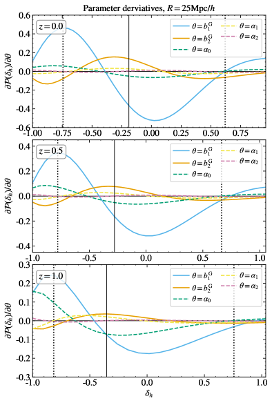
Figure 20: Halo PDF derivatives w.r.t. the renormalised Lagrangian Gaussian bias and quadratic shot noise parameters.

B.4 Tracer power spectra

We show the performance of our simplistic halo power spectrum modelling for the fiducial cosmology in Figure 21. The derivatives of the halo and mock galaxy power spectra with respect to cosmological and bias parameters are shown in Figures 23 and 23, respectively. As expected, the parameters $\sigma_{8}$ and $\beta$ control the amplitude of the power spectrum such that their shape closely reflects the shape of the power spectrum. The spectral index $n_{s}$ additionally leads to a change in the scale dependence. The matter density $\Omega_{m}$ modulates the large-scale power through the growth factor leading to larger differences at larger redshifts. Additionally, it modifies the Baryon Acoustic Oscillation wiggles in the matter power spectrum, which get washed out by the scale-dependent bias and shot noise. We checked that despite its simplicity, our tracer power spectrum model (28) reproduces the cosmology and bias constraints obtained from the simulated power spectra. For the case of constraints at a single redshift, the constraints on the amplitude parameters $\sigma_{8}$ and $\beta$ are very weak, while the theory provides marginally stronger results. This becomes insignificant when adding several redshifts, as the shared cosmological parameters become more tightly constrained. This cross-validation demonstrates the convergence of the simulated power spectrum derivatives and the sufficiency of the simplistic modelling given the parameters of interest.

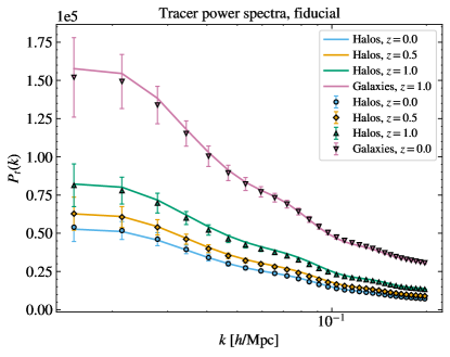
Figure 21: Halo and galaxy power spectra as measured from the fiducial Quijote simulations or Molino catalogues (data points) and predicted from the model (28) (solid lines).

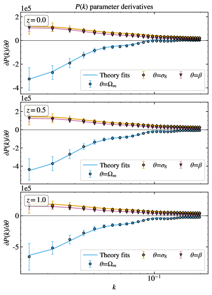
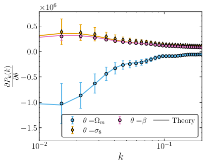
Figure 22: Halo power spectrum derivatives w.r.t. cosmological and combined bias and shot noise parameters (data points) and prediction from the simplistic two-parameter model (28) with fixed parameters across cosmologies (solid lines).

Figure 23: Galaxy power spectrum derivatives w.r.t. cosmological and combined bias and shot noise parameters. The data points represent the derivatives computed from Molino measurements of the galaxy power spectrum. The solid lines represent the predictions from the theoretical model presented in equation (28).

B.5 Fisher forecast: Gaussianity of data vector

The validity of the Fisher analysis relies on the assumption of Gaussian likelihood. Here, we verify the validity of our Fisher analysis by testing the Gaussian distribution of the bins in the halo Quijote PDF across different realisations. We achieve this by computing histograms of the fluctuation of the bin values relative to the mean, divided by the standard deviation. Since bins located at the low and high density regions can potentially deviate from Gaussianity, Figure 24 illustrates how the halo PDF bins for the minimum and maximum $\delta_{h}$ values we consider at redshift $z=0.0$ and for the three smoothing scales $R=20.0,25.0,30.0$Mpc$/h$ follow a Gaussian distribution with a mean given by the average over realisations and a variance determined by the diagonal of the covariance matrix. We also verify that other bins follow a Gaussian distribution, obtaining similar results for the other redshifts.

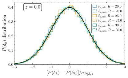
Figure 24: Gaussianity test of the halo PDF data bins. Histogram of the fluctuations of the bin values relative to the mean, divided by the standard deviation across $15,000$ realisations of the halo Quijote simulations at redshift $z=0$. Histogram of the distribution of halo PDF values for the minimum (solid lines) and maximum (dashed lines) $\delta_{h}$ for three smoothing scales$R=20.0,25.0,30.0$ Mpc$/h$ (blue, orange and green lines respectively). The solid black line represents a Gaussian distribution with mean zero and unit variance.

To validate the full data vector and the inverse covariance used in the Fisher forecast we perform a $\chi^{2}-$test. We employ the following expression

$$\chi^{2}=\frac{1}{2}\left(S_{\alpha}-\langle S_{\alpha}\rangle\right)C_{\alpha\beta}^{-1}\left(S_{\beta}-\langle S_{\beta}\rangle\right)\,,$$ (54)

and plot histograms of the $\chi^{2}$ values.

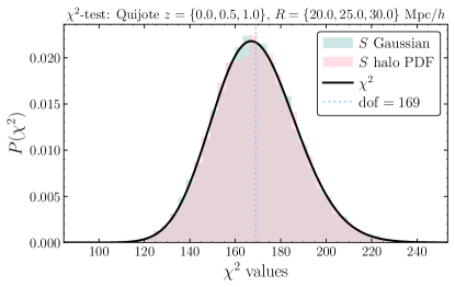
Figure 25: Distribution of $\chi^{2}-$values combining three redshifts $z=0.0,0.5,1.0$ and three smoothing scales $R=20.0,25.0,30.0$Mpc$/h$ for each redshift (pink histogram). The distribution follows a $\chi^{2}-$distribution with the same number of degrees of freedom (dof) (black line). $\chi^{2}-$values distribution for a data vector, build from a Gaussian distribution with same mean and covariance as data vector for the halo PDF (blue histograms).

The data vector $\vec{S}$ combines the Quijote halo one-point PDF at three redshifts $z=0.0,0.5,1.0$ and three smoothing scales $R=20.0,25.0,30.0$Mpc$/h$ for each redshift. The covariance is estimated using $15,000$ realisations of the fiducial Quijote halo PDF. Figure 25 confirms that the $\chi^{2}$-values follow a $\chi^{2}$ distribution, validating the accuracy of the inverse covariance. Additionally, we show the $\chi^{2}$-values distribution considering a data vector build from a Gaussian distribution with the same mean and covariance as the Quijote halo PDF data vector which also follows the $\chi^{2}$ distribution supporting the applicability of the Fisher forecast in section 4.4.

B.6 Convergence of Fisher forecasts

In Figure 26 we check the convergence of the Fisher forecasts for the parameters $\{\Omega_{m},\sigma_{8},\beta_{z}\}$. We vary both the number of realisations used for computing the data covariance and the number of realisations used for computing the data derivatives. The effect of super-sample covariance is not included here, which accounts for the slight difference to Figure 17.

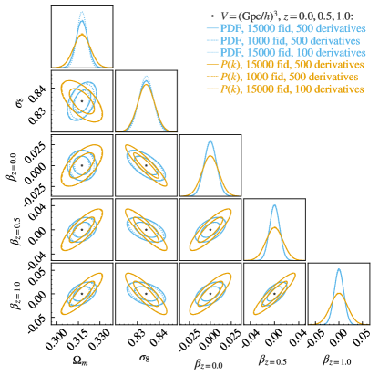
Figure 26: Fisher forecast for halo PDF (blue) and power spectrum (red) as measured from Quijote using 15000 fiducial realisations and 500 derivative realisations (solid), 1000 fiducial realisations and 500 derivative realisations (dashed) and 5000 fiducial realisations and 100 derivative realisations (dotted).

We find robustness with respect to reducing the realisations used for estimating the covariance. In contrast, we find a significant dependence of the obtained constraints on the number of realisations used to estimate the derivatives indicating artificial degeneracy breaking due to numerical noise. This effect would be further exacerbated when marginalising over the bias parameters, which is why we decide to reduce the number of cosmological parameters we vary. An alternative avenue would be to use the approach of Coulton and Wandelt (2023) to obtain conservative estimates and use compression to limit the impact of numerical noise.

References

- Aghamousa et al. (2016) A. Aghamousa et al. (DESI), (2016), arXiv:1611.00036 [astro-ph.IM] .
- Laureijs et al. (2011) R. Laureijs et al. (EUCLID), (2011), arXiv:1110.3193 [astro-ph.CO] .
- Takahashi et al. (2012) R. Takahashi, M. Sato, T. Nishimichi, A. Taruya, and M. Oguri, ApJ 761, 152 (2012), arXiv:1208.2701 .
- Knabenhans et al. (2021) M. Knabenhans et al., Monthly Notices of the Royal Astronomical Society 505, 2840–2869 (2021).
- Donald-McCann et al. (2022) J. Donald-McCann, F. Beutler, K. Koyama, and M. Karamanis, MNRAS 511, 3768 (2022), arXiv:2109.15236 [astro-ph.CO] .
- Bernardeau et al. (2002) F. Bernardeau, S. Colombi, E. Gaztañaga, and R. Scoccimarro, Phys. Rep. 367, 1 (2002), arXiv:astro-ph/0112551 [astro-ph] .
- Carrasco et al. (2012) J. J. M. Carrasco, M. P. Hertzberg, and L. Senatore, JHEP 09, 082 (2012), arXiv:1206.2926 [astro-ph.CO] .
- Porto et al. (2014) R. A. Porto, L. Senatore, and M. Zaldarriaga, JCAP 05, 022 (2014), arXiv:1311.2168 [astro-ph.CO] .
- Gil-Marín et al. (2015) H. Gil-Marín, J. Noreña, L. Verde, W. J. Percival, C. Wagner, M. Manera, and D. P. Schneider, Monthly Notices of the Royal Astronomical Society 451, 539–580 (2015).
- Alam et al. (2017) S. Alam et al., MNRAS 470, 2617 (2017), arXiv:1607.03155 [astro-ph.CO] .
- Beutler et al. (2017) F. Beutler et al., MNRAS 466, 2242 (2017), arXiv:1607.03150 [astro-ph.CO] .
- Satpathy et al. (2017) S. Satpathy et al., MNRAS 469, 1369 (2017), arXiv:1607.03148 [astro-ph.CO] .
- Sánchez et al. (2017) A. G. Sánchez et al., MNRAS 464, 1640 (2017), arXiv:1607.03147 [astro-ph.CO] .
- D’Amico et al. (2020) G. D’Amico, J. Gleyzes, N. Kokron, K. Markovic, L. Senatore, P. Zhang, F. Beutler, and H. Gil-Marín, JCAP 05, 005 (2020), arXiv:1909.05271 [astro-ph.CO] .
- Ivanov et al. (2020) M. M. Ivanov, M. Simonović, and M. Zaldarriaga, JCAP 05, 042 (2020), arXiv:1909.05277 [astro-ph.CO] .
- Colas et al. (2020) T. Colas, G. D’amico, L. Senatore, P. Zhang, and F. Beutler, JCAP 06, 001 (2020), arXiv:1909.07951 [astro-ph.CO] .
- D’Amico et al. (2024) G. D’Amico, Y. Donath, M. Lewandowski, L. Senatore, and P. Zhang, JCAP 05, 059 (2024), arXiv:2206.08327 [astro-ph.CO] .
- Uhlemann et al. (2020) C. Uhlemann, O. Friedrich, F. Villaescusa-Navarro, A. Banerjee, and S. Codis, Monthly Notices of the Royal Astronomical Society 495, 4006 (2020).
- Banerjee and Abel (2021a) A. Banerjee and T. Abel, MNRAS 500, 5479 (2021a), arXiv:2007.13342 [astro-ph.CO] .
- Bernardeau and Reimberg (2015) F. Bernardeau and P. Reimberg, Physical Review D 94 (2015), 10.1103/PhysRevD.94.063520.
- Uhlemann et al. (2015) C. Uhlemann, S. Codis, C. Pichon, F. Bernardeau, and P. Reimberg, Monthly Notices of the Royal Astronomical Society (2015), 10.1093/mnras/stw1074.
- Friedrich et al. (2020a) O. Friedrich, C. Uhlemann, F. Villaescusa-Navarro, T. Baldauf, M. Manera, and T. Nishimichi, Mon. Not. Roy. Astron. Soc. 498, 464 (2020a), arXiv:1912.06621 [astro-ph.CO] .
- Coulton et al. (2023) W. R. Coulton, T. Abel, and A. Banerjee, arXiv e-prints , arXiv:2309.15151 (2023), arXiv:2309.15151 [astro-ph.CO] .
- Cataneo et al. (2022) M. Cataneo, C. Uhlemann, C. Arnold, A. Gough, B. Li, and C. Heymans, MNRAS 513, 1623 (2022), arXiv:2109.02636 [astro-ph.CO] .
- Coles and Jones (1991) P. Coles and B. Jones, MNRAS 248, 1 (1991).
- Bel et al. (2016) J. Bel et al., A&A 588, A51 (2016), arXiv:1505.00442 [astro-ph.CO] .
- Clerkin et al. (2017) L. Clerkin et al., MNRAS 466, 1444 (2017), arXiv:1605.02036 [astro-ph.CO] .
- Hurtado-Gil et al. (2017) L. Hurtado-Gil, V. J. Martínez, P. Arnalte-Mur, M.-J. Pons-Bordería, C. Pareja-Flores, and S. Paredes, Astronomy & Astrophysics 601, A40 (2017).
- Friedrich et al. (2018) O. Friedrich et al. (DES), Phys. Rev. D 98, 023508 (2018), arXiv:1710.05162 [astro-ph.CO] .
- Gruen et al. (2018) D. Gruen et al. (DES), Phys. Rev. D 98, 023507 (2018), arXiv:1710.05045 [astro-ph.CO] .
- Repp and Szapudi (2020) A. Repp and I. Szapudi, Monthly Notices of the Royal Astronomical Society: Letters 498, L125 (2020), arXiv: 2006.01146.
- Barthelemy et al. (2020) A. Barthelemy, S. Codis, C. Uhlemann, F. Bernardeau, and R. Gavazzi, Monthly Notices of the Royal Astronomical Society 492, 3420–3439 (2020).
- Thiele et al. (2020) L. Thiele, J. C. Hill, and K. M. Smith, Physical Review D 102 (2020), 10.1103/physrevd.102.123545.
- Barthelemy et al. (2021) A. Barthelemy, S. Codis, and F. Bernardeau, Monthly Notices of the Royal Astronomical Society 503, 5204–5222 (2021).
- Boyle et al. (2020) A. Boyle, C. Uhlemann, O. Friedrich, A. Barthelemy, S. Codis, F. Bernardeau, C. Giocoli, and M. Baldi, arXiv:2012.07771 [astro-ph] (2020), arXiv: 2012.07771.
- Barthelemy et al. (2024) A. Barthelemy, A. Halder, Z. Gong, and C. Uhlemann, J. Cosmology Astropart. Phys 2024, 060 (2024), arXiv:2307.09468 [astro-ph.CO] .
- Castiblanco et al. (2024) L. Castiblanco, C. Uhlemann, J. Harnois-Déraps, and A. Barthelemy, The Open Journal of Astrophysics 7 (2024), 10.33232/001c.121302.
- Sreekanth et al. (2024) V. T. Sreekanth, S. Codis, A. Barthelemy, and J.-L. Starck, “Theoretical wavelet -norm from one-point pdf prediction,” (2024), arXiv:2406.10033 [astro-ph.CO] .
- Friedrich et al. (2020b) O. Friedrich, C. Uhlemann, F. Villaescusa-Navarro, T. Baldauf, M. Manera, and T. Nishimichi, Mon. Not. Roy. Astron. Soc. 498, 464 (2020b), arXiv:1912.06621 [astro-ph.CO] .
- Ivanov et al. (2019) M. M. Ivanov, A. A. Kaurov, and S. Sibiryakov, Journal of Cosmology and Astroparticle Physics 2019, 009–009 (2019).
- Chudaykin et al. (2023) A. Chudaykin, M. M. Ivanov, and S. Sibiryakov, “Renormalizing one-point probability distribution function for cosmological counts in cells,” (2023), arXiv:2212.09799 [astro-ph.CO] .
- Villaescusa-Navarro et al. (2019) F. Villaescusa-Navarro et al., arXiv:1909.05273 [astro-ph] (2019), arXiv: 1909.05273.
- Davis et al. (1985) M. Davis, G. Efstathiou, C. S. Frenk, and S. D. M. White, The Astrophysical Journal 292, 371 (1985).
- Seljak et al. (2009) U. Seljak, N. Hamaus, and V. Desjacques, Phys. Rev. Lett. 103, 091303 (2009), arXiv:0904.2963 [astro-ph.CO] .
- Hamaus et al. (2010) N. Hamaus, U. Seljak, V. Desjacques, R. E. Smith, and T. Baldauf, Phys. Rev. D 82, 043515 (2010), arXiv:1004.5377 [astro-ph.CO] .
- Jee et al. (2012) I. Jee, C. Park, J. Kim, Y.-Y. Choi, and S. S. Kim, ApJ 753, 11 (2012), arXiv:1204.5573 [astro-ph.CO] .
- Uhlemann et al. (2018) C. Uhlemann, M. Feix, S. Codis, C. Pichon, F. Bernardeau, B. L’Huillier, J. Kim, S. E. Hong, C. Laigle, C. Park, J. Shin, and D. Pogosyan, Monthly Notices of the Royal Astronomical Society 473, 5098 (2018), arXiv: 1705.08901.
- Hahn and Villaescusa-Navarro (2021) C. Hahn and F. Villaescusa-Navarro, JCAP 04, 029 (2021), arXiv:2012.02200 [astro-ph.CO] .
- Zheng et al. (2007) Z. Zheng, A. L. Coil, and I. Zehavi, The Astrophysical Journal 667, 760 (2007), arXiv: astro-ph/0703457.
- Uhlemann et al. (2018) C. Uhlemann, C. Pichon, S. Codis, B. L’Huillier, J. Kim, F. Bernardeau, C. Park, and S. Prunet, MNRAS 477, 2772 (2018), arXiv:1711.04767 [astro-ph.CO] .
- Friedrich et al. (2022) O. Friedrich, A. Halder, A. Boyle, C. Uhlemann, D. Britt, S. Codis, D. Gruen, and C. Hahn, MNRAS 510, 5069 (2022), arXiv:2107.02300 [astro-ph.CO] .
- Banerjee et al. (2022) A. Banerjee, N. Kokron, and T. Abel, MNRAS 511, 2765 (2022), arXiv:2107.10287 [astro-ph.CO] .
- Britt et al. (2024) D. Britt, D. Gruen, O. Friedrich, S. Yuan, and B. Ried Guachalla, arXiv e-prints , arXiv:2404.04252 (2024), arXiv:2404.04252 [astro-ph.CO] .
- Banerjee and Abel (2021b) A. Banerjee and T. Abel, MNRAS 504, 2911 (2021b), arXiv:2102.01184 [astro-ph.CO] .
- Banerjee and Abel (2023) A. Banerjee and T. Abel, MNRAS 519, 4856 (2023), arXiv:2210.05140 [astro-ph.CO] .
- Fry and Gaztanaga (1993) J. N. Fry and E. Gaztanaga, ApJ 413, 447 (1993), arXiv:astro-ph/9302009 [astro-ph] .
- Manera and Gaztañaga (2011) M. Manera and E. Gaztañaga, MNRAS 415, 383 (2011), arXiv:0912.0446 [astro-ph.CO] .
- Salvador et al. (2019) A. I. Salvador et al. (DES), Mon. Not. Roy. Astron. Soc. 482, 1435 (2019), arXiv:1807.10331 [astro-ph.CO] .
- Desjacques et al. (2018) V. Desjacques, D. Jeong, and F. Schmidt, Phys. Rep. 733, 1 (2018), arXiv:1611.09787 [astro-ph.CO] .
- Sheth et al. (2001) R. K. Sheth, H. J. Mo, and G. Tormen, Monthly Notices of the Royal Astronomical Society 323, 1–12 (2001).
- Press and Schechter (1974) W. H. Press and P. Schechter, ApJ 187, 425 (1974).
- Wagner et al. (2015) C. Wagner, F. Schmidt, C.-T. Chiang, and E. Komatsu, J. Cosmology Astropart. Phys 2015, 042 (2015), arXiv:1503.03487 [astro-ph.CO] .
- Lazeyras et al. (2016) T. Lazeyras, C. Wagner, T. Baldauf, and F. Schmidt, Journal of Cosmology and Astroparticle Physics 2016, 018–018 (2016).
- Stücker et al. (2024a) J. Stücker, M. Pellejero-Ibáñez, R. Voivodic, and R. E. Angulo, arXiv e-prints , arXiv:2405.01951 (2024a), arXiv:2405.01951 [astro-ph.CO] .
- Stücker et al. (2024b) J. Stücker, M. Pellejero-Ibáñez, R. E. Angulo, F. Maion, and R. Voivodic, arXiv e-prints , arXiv:2405.01950 (2024b), arXiv:2405.01950 [astro-ph.CO] .
- Uhlemann et al. (2022) C. Uhlemann, O. Friedrich, A. Boyle, A. Gough, A. Barthelemy, F. Bernardeau, and S. Codis, Open J. Astrophys. 6, 2023 (2022), arXiv:2210.07819 [astro-ph.CO] .
- Bernardeau and Valageas (2000) F. Bernardeau and P. Valageas, A&A 364, 1 (2000), arXiv:astro-ph/0006270 [astro-ph] .
- Bernardeau et al. (2014) F. Bernardeau, C. Pichon, and S. Codis, Physical Review D 90 (2014), 10.1103/physrevd.90.103519.
- Codis et al. (2016) S. Codis, F. Bernardeau, and C. Pichon, Monthly Notices of the Royal Astronomical Society 460, 1598–1613 (2016).
- Kaufman (1967) G. M. Kaufman, Report No. 6710, Center for Operations Research and Econometrics, Catholic University of Louvain, Heverlee, Belgium (1967).
- Hartlap et al. (2007) J. Hartlap, P. Simon, and P. Schneider, Astron. Astrophys. 464, 399 (2007), arXiv:astro-ph/0608064 .
- Sirko (2005) E. Sirko, ApJ 634, 728 (2005), arXiv:astro-ph/0503106 [astro-ph] .
- Yuan et al. (2023) S. Yuan, A. Zamora, and T. Abel, MNRAS 522, 3935 (2023), arXiv:2304.10565 [astro-ph.CO] .
- Hunter et al. (2007) J. D. Hunter et al., Computing in Science & Engineering 9, 90 (2007).
- Harris et al. (2020) C. R. Harris et al., Nature 585, 357 (2020).
- Virtanen et al. (2020) P. Virtanen et al., Nature Methods 17, 261 (2020).
- Hinton (2016) S. R. Hinton, The Journal of Open Source Software 1, 00045 (2016).
- Coulton and Wandelt (2023) W. R. Coulton and B. D. Wandelt, arXiv e-prints , arXiv:2305.08994 (2023), arXiv:2305.08994 [stat.ME] .