Tuning transport in solid-state Bose-Fermi mixtures by Feshbach resonances

Abstract

Transition metal dichalcogenide (TMD) heterostructures have emerged as promising platforms for realizing tunable Bose-Fermi mixtures. Their constituents are fermionic charge carriers resonantly coupled to long-lived bosonic interlayer excitons, allowing them to form trion bound states. Such platforms promise to achieve comparable densities of fermions and bosons at low relative temperatures. Here, we predict the transport properties of Bose-Fermi mixtures close to a narrow solid-state Feshbach resonance. When driving a hole current, the response of doped holes, excitons, and trions are significantly modified by the resonant interactions, leading to deviations from the typical Drude behavior and to a sign change of the exciton drag. Our results on the temperature-dependent resistivities demonstrate that interaction effects dominate over established conventional scattering mechanisms in these solid-state Bose-Fermi mixtures.

Unconventional phases in solids are predicted to arise when a Fermi surface is strongly coupled to bosonic excitations, such as phonons, spin- and density-wave fluctuations, and collective modes emerging in the vicinity of phase transitions [1, 2, 3, 4, 5, 6, 7, 8]. However, isolating relevant interaction channels is challenging, as electrons are typically coupled simultaneously to multiple bosonic modes. This motivates the exploration of Bose-Fermi mixtures in more controlled settings of transition-metal-dichalcogenide (TMD) heterostructures [9, 10, 11, 12, 13, 14, 15, 16]; complementary regimes are accessible in ultracold atomic gases as well [17, 18, 19, 20, 21, 22]. TMDs offer the advantage that low relative temperatures are reachable [15]. In these settings, fermions are introduced by charge doping and high densities of long-lived bosons are realized as tightly-bound interlayer excitons [23]. Excitons interact with doped charges [24, 10, 25, 26] forming fermionic bound states, referred to as trions, which have been observed to remain stable even at finite densities [15, 16]. As low-temperature Bose-Fermi mixtures are now becoming accessible in experiments, both understanding signatures of many-body scattering and accomplishing additional control over interactions are crucial for exploring the phases and their properties.

In this work, we theoretically investigate transport properties of tunable solid-state Bose-Fermi mixtures in TMD heterostructures. We consider a selectively driven hole current, and show that resonant exciton-hole scattering and trion formation lead to strong modifications of the conductivities of all three particle species. In analogy with cold atomic gases, we exploit the control of exciton-charge scattering by a solid-state Feshbach resonance, and thus scattering depends sensitively on the trion energy which is tunable by a perpendicular electric field [26, 10, 27]. Remarkably, exciton-hole scattering dominates the transport properties below the phonon temperature scale, and induces a sign-changing exciton drag conductivity in a broad parameter regime. As another striking effect we find that the resistivity of the system exhibits a strong, non-monotonic temperature dependence, as well as an unconventional ac response beyond Drude phenomenology.

Model.— Inspired by recent experiments [10, 15, 16], we propose a setting composed of three monolayer TMDs, where the top layer is hole-doped and separated from the other layers by hexagonal boron nitride (hBN) with a thickness $d$, see Fig. 1 (a). The relative energy of charges in the middle layer is tuned by a perpendicular electric field $E_{z}$. This imposes an electrostatic potential difference $eE_{z}d$, where $e$ is the elementary charge. We consider fields $E_{z}$ that increase the trion energy and suppress tunneling of unbound holes to the middle layer, see Fig. 1 (a,b). Interlayer excitons form in between the middle and the lower layer. Due to the small overlap of hole and electron wavefunctions, their lifetime can exceed hundreds of ns, which allows us to treat excitons as well-defined bosonic particles [23].

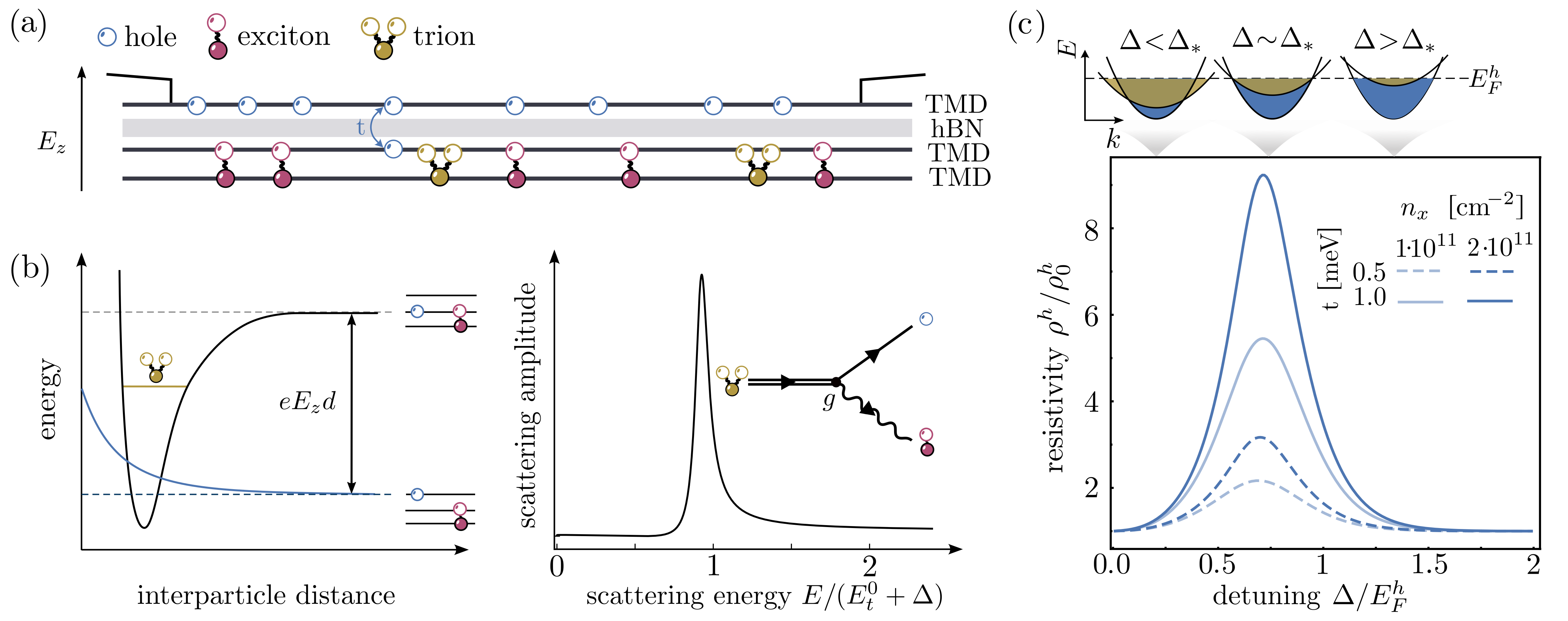
Figure 1: Setup, particle-like trion bound state and enhanced transport close to resonance. a) Proposed trilayer TMD structure. The system realizes a Bose-Fermi mixture with doped charges (holes) in the upper layer and strongly bound interlayer excitons in the lower two layers. A longitudinal electric field is applied only to the top layer via direct contacts that drive a hole current. b) Solid-state Feshbach resonance. Left: The energy of a spatially separated exciton-hole pair (blue curve) can be tuned close to the energy of the trion (yellow) by the perpendicular electric field, which shifts the energy of the trion to $E_{t}^{0}+\Delta=eE_{z}d$. Right: The exciton-hole scattering amplitude is resonantly enhanced around the shifted trion energy due to the narrow Feshbach resonance. c) Resistivity of holes in the upper layer $\rho^{h}$ as a function of the detuning $\Delta$, calculated at $T=5.8$ K. The resistivity is strongly enhanced close to the resonance condition $\Delta=\Delta_{\star}$, where the hole and trion Fermi surfaces have the same size. Top: Sketches to illustrate the hole and trion Fermi seas as a function of $\Delta$.

The resulting system is well described by holes, excitons and trions with quadratic dispersions $\epsilon_{h,\mathbf{p}}=\frac{\mathbf{p}^{2}}{2m_{h}}-\mu_{h}$, $\omega_{\mathbf{k}}=\frac{\mathbf{k}^{2}}{2m_{x}}-\mu_{x}$ and $\epsilon_{t,\mathbf{p}}=\frac{\mathbf{p}^{2}}{2m_{t}}-\mu_{t}+\Delta$, respectively, where $\Delta=eE_{z}d-E_{t}^{0}$, with $E_{t}^{0}$ the trion binding energy. The trion mass is $m_{t}=m_{x}+m_{h}$. We assume the system has reached thermal equilibrium, which fixes the chemical potentials to satisfy $\mu_{h}+\mu_{x}=\mu_{t}$ [28]. The effective Hamiltonian describing the solid-state Bose-Fermi mixture is then

$$\hat{H} =\!\!\int\!\!\!\tfrac{\mathrm{d}^{2}\mathbf{p}}{(2\pi)^{2}}\left(\epsilon_{h,\mathbf{p}}\,\hat{c}^{\dagger}_{\mathbb{p}}\hat{c}_{\mathbb{p}}+\epsilon_{t,\mathbf{p}}\,\hat{m}^{\dagger}_{\mathbb{p}}\hat{m}_{\mathbb{p}}\right)\!+\!\!\int\!\!\!\tfrac{\mathrm{d}^{2}\mathbf{k}}{(2\pi)^{2}}\,\omega_{\mathbf{k}}\,\hat{x}^{\dagger}_{\mathbb{k}}\hat{x}_{\mathbb{k}}$$ (1)

$$+g\int\!\!\!\tfrac{\mathrm{d}^{2}\mathbf{p}}{(2\pi)^{2}}\tfrac{\mathrm{d}^{2}\mathbf{k}}{(2\pi)^{2}}\left(\hat{m}^{\dagger}_{\mathbb{p}+\mathbb{k}}\hat{c}_{\mathbb{p}}\hat{x}_{\mathbb{k}}+\text{h.c.}\right),$$

where $\hat{c}^{\dagger},\hat{x}^{\dagger}$ and $\hat{m}^{\dagger}$ ($\hat{c},\hat{x}$ and $\hat{m}$) are the hole, exciton and trion creation (annhilation) operators, and $g$ is the effective coupling strength. Starting from the microscopic exciton-hole Hamiltonian, we estimate $g\simeq\left(\frac{2\pi}{m_{\text{red}}|E_{t}^{0}|}\right)^{1/2}{\rm t}$, where $\rm t$ is the hole coherent tunneling rate, $E_{t}^{0}$ is the bare trion energy, $m_{\text{red}}^{-1}=m_{h}^{-1}+m_{x}^{-1}=(3/2)\,m_{h}^{-1}$, and we have assumed that $g$ is momentum-independent [18, 29, 26]. For $\Delta\geq 0$, the trion decays into an exciton-hole pair at a rate proportional to $\rm t^{2}$, which can be much smaller than the relevant Fermi energies [10]. This allows us to treat trions as sharp quasi-particles whose energy is tuned by a Feshbach resonance, see Fig. 1 (b). Even for finite hole and exciton densities, the trion retains a quasi-particle peak, provided $g\ll E_{F}^{h}/\sqrt{n_{x}}$, which we use as a perturbative parameter to study transport.

Unless stated otherwise, we will use the following parameters: hole Fermi energy $E_{F}^{h}=5$ meV, $E_{t}^{0}=-10$ meV, $\rm t=1$ meV, $n_{x}=2\cdot 10^{11}$ cm^-2 and $m_{h}=0.5\,m_{\sf e}$ with $m_{\sf e}$ the free electron mass [30, 10, 31, 15, 16]. Throughout the paper we take $\hbar=1$, and model extrinsic sources of momentum relaxation (e.g. disorder) for all species by a momentum-independent relaxation time $\tau_{0}=10$ ps, motivated by recent transport experiments [32, 33, 34].

Methods.— Electrical contacts are placed such that a longitudinal electric field is applied only to the charge-doped layer, as shown in Fig. 1(a). This induces a charge current $j^{h}_{a}=\sigma^{h}_{ab}E_{b}$ in the upper layer, where $\sigma^{h}_{ab}$ is the hole conductivity tensor and $a,b\in\{x,y\}$ are the longitudinal and transverse directions. Since we are considering linear response in an isotropic and time-reversal symmetric model, $\sigma^{h}_{ab}=\delta_{ab}/\rho^{h}$ with $\rho^{h}$ the hole resistivity. Excitons and trions do not couple to the electric field directly. Instead, their particle currents, $J_{a}^{x}$ and $J_{a}^{t}$, induced in the middle and lower layers, arise purely from drag effects mediated by the hole current via many-body scattering. We define the corresponding conductivity as $\sigma^{i}_{ab}=eJ^{i}_{a}/E_{b}$ for $i\in\{x,t\}$. We analyze the currents induced in the system for all three species of particles, as a function of detuning $\Delta$ and temperature $T$. Using a kinetic theory approach, where the collision integrals are obtained from a perturbative calculation of the self-energies [35], we derive and solve a set of three coupled Boltzmann’s equations for the particle distributions. A perturbative calculation of the hole conductivity based on Kubo’s formula [36] yields similar results, up to quantitative corrections in the vicinity of the resonance. Further details about both methods, and a comparison, are reported in the Supplemental Material [37].

Tunable hole transport.—

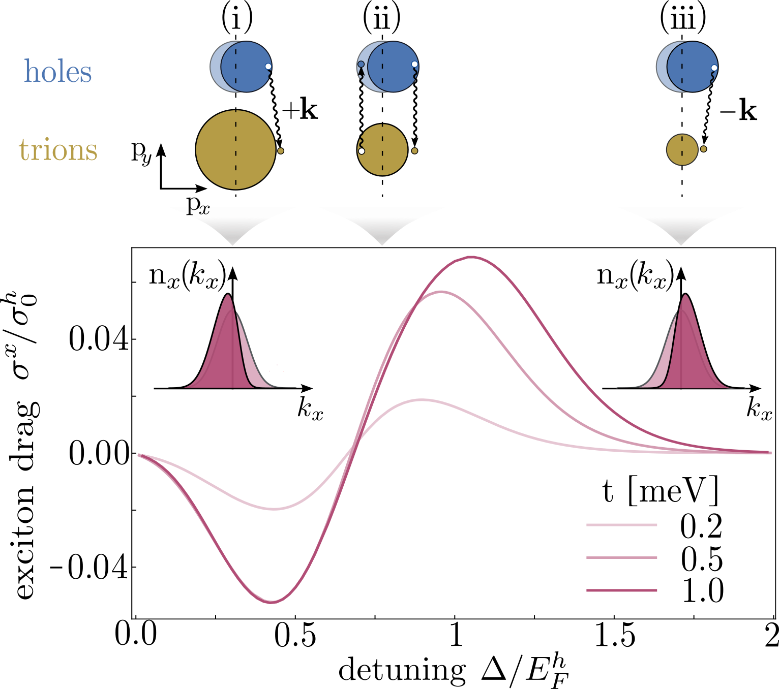
Figure 2: Sign-changing exciton drag. Exciton drag conductivity as a function of detuning $\Delta$ evaluated at temperature $T=5.8$ K. The backflow of excitons, $\sigma^{x}<0$, for small detuning can be understood from the interplay of energy and momentum conservation and Pauli exclusion. Upper panels: Sketches of the relevant scattering processes for exciton drag. (i) A hole (from the blue Fermi sea) absorbs a right-moving exciton (squiggly arrow) to form a trion (above the yellow Fermi sea). This depletes right-moving excitons and skews the exciton distribution $n_{x}(k_{x})$ (red) against the direction of the hole current. (ii) Close to resonance, scattering processes primarily involve small-momentum excitons, leading to a small exciton drag. (iii) A hole absorbs a left-moving excition, which skews the exciton distribution $n_{x}(k_{x})$ in the direction of the hole current.

In our system, holes exhibit a tunable resistivity $\rho^{h}$: the resistivity $\rho^{h}$ is governed not only by the intrinsic background scattering rate $\tau_{0}^{-1}$ that sets the constant background resistivity $\rho^{h}_{0}=2\pi/(\mu_{h}e^{2}\tau_{0})=1/\sigma_{0}^{h}$, but crucially also by many-body interactions with the bosonic interlayer excitons that depend on the perpendicular electric field $E_{z}=(\Delta+E_{t}^{0})/ed$. By solving the coupled transport equations, we find that the resistivity $\rho^{h}$ exhibits a strong resonant behaviour as a function of the detuning $\Delta$, as demonstrated in Fig. 1(c) for different tunneling rates $\rm t$ and exciton densities $n_{x}$. The tunability of the resistivity originates from exciton-hole scattering, as the perpendicular electric field $E_{z}$ sweeps through the Feshbach resonance and sets the size of the trion Fermi surface. For small $\Delta$ the trion Fermi surface is large, and shrinks for larger values of $\Delta$ until it eventually vanishes for $\Delta\gtrsim\mu_{h}$. The contribution of interactions to the hole resistivity is determined by the hole many-body scattering rate, which to order $O(g^{2})$ reads

$$\text{Im}\Sigma^{R}_{h}(\mathbb{p},\epsilon_{h,\mathbb{p}}) =|g|^{2}\!\int\!\tfrac{\mathrm{d}^{2}\mathbf{k}}{(2\pi)^{2}}\big{(}n_{F}(\epsilon_{t,\mathbf{p}+\mathbf{k}})+n_{B}(\omega_{\mathbf{k}})\big{)}$$ (2)

$$\qquad\times 2\pi\,\delta(\omega_{\mathbf{k}}+\epsilon_{h,\mathbf{p}}-\epsilon_{t,\mathbf{p}+\mathbf{k}}),$$

with $n_{B}$ and $n_{F}$ the Bose and Fermi distributions. The conservation of energy in Eq. (2) ensures that the trion energy matches the combined energies of the exciton and hole. This captures the dominant contribution of the resonant peak to the scattering amplitude shown in Fig. 1(b), and reflects the existence of a metastable Feshbach molecule.

At low temperatures, Eq. (2) is dominated by processes involving small exciton momentum $\mathbf{k}$, where the bosonic population $n_{B}(\omega_{\mathbf{k}})$ is largest. Many-body scattering is then maximized when the energy of a trion is resonant with the energy of a hole nearby the Fermi surface. In our model this takes place when the two Fermi surfaces are of the same size, which occurs when $\Delta$ is tuned to

$$\Delta_{\star}=\big{(}1-m_{h}/m_{t}\big{)}\,\mu_{h}=(2/3)\,\mu_{h}.$$ (3)

We find that tuning the electric field on resonance strongly enhances the hole resistivity by about an order of magnitude, see Fig. 1(c). The background Drude resistivity $\rho_{0}^{h}$ is recovered in the limit $\Delta\leq 0$, where the phase space volume satisfying the constraint in Eq. (2) vanishes, and for sufficiently strong detuning $\Delta\gg 1$ as scattering becomes off-resonant.

Interaction induced drag transport.— Although excitons are charge neutral and spatially decoupled from the driven layer, they experience drag effects due to exciton-hole scattering. The resulting drag conductivity $\sigma^{x}$ can be experimentally measured by separately contacting the lower two layers. Because it is entirely interaction-driven, the exciton conductivity is highly tunable with the electric field. Three distinct regimes are identified (Fig. 2):

(i) For $\Delta<\Delta_{\star}$ the hole Fermi surface is smaller than the trion Fermi surface. Thus holes driven out of equilibrium with $p_{x}>0$ combine mainly with excitons carrying positive momenta $k_{x}>0$, depleting the exciton distribution for $k_{x}>0$. This results in an exciton current $J^{x}_{x}<0$ that flows in the opposite direction to the hole current.

(ii) For $\Delta\simeq\Delta_{\star}$ the exciton drag $\sigma^{x}$ vanishes and changes sign. Dominant scattering results from excitons with small momenta, which carry negligible current. This is in stark contrast with the hole resistivity for which many-body scattering is most dominant in this regime.

(iii) For $\Delta>\Delta_{\star}$, the trion Fermi surface is smaller than the hole Fermi surface. Thus holes with $p_{x}>0$ dominantly combine with excitons with $k_{x}<0$, depleating the exciton distribution for $k_{x}<0$, which yields an exciton current $J^{x}_{x}>0$ flowing in the direction of the hole current.

The exciton drag increases with the hybridization $\rm t$, see Fig. 2. Since excitons are charge neutral, their conductivity scales to leading order as $\sigma^{x}\sim g^{2}/\rho^{h}$. Away from resonance and for small tunneling rates $t\ll 1/\tau_{0}$ the hole resistivity remains close to its background value $\rho^{h}\approx\rho_{0}^{h}+O(g^{2})$. Consequently, the exciton conductivity follows $\sigma^{x}\sim g^{2}/\rho_{0}\sim{\rm t}^{2}/\rho_{0}$, as $g\sim\rm t$. Near resonance, however, the hole resistivity is governed by many-body scattering, which also scales as $\rho^{h}\sim\rm{t}^{2}$. This implies a saturation of $\sigma^{x}$ with increasing tunneling $\rm t$, see Fig. 2. This intuitive picture, which focuses on the thermally dominant scattering processes, is confirmed by our calculations, which systematically include all such scattering processes, as detailed in the Supplemental Material [37]. Our mechanism should be distinguished from exciton drag resulting from polaron formation in monolayer settings [38].

Non-monotonous temperature dependence.—

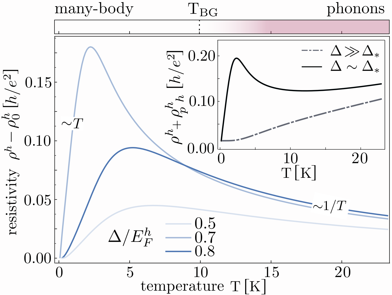
Figure 3: Temperature dependence of the hole resistivity. Many-body contribution to the resistivity $\rho^{h}-\rho^{h}_{0}$ as a function of temperature $T$ for different detunings $\Delta$, where $\rho^{h}_{0}=2\pi/\mu_{h}e^{2}\tau_{0}$ is the Drude resistivity at zero temperature. Inset: Total resistivity $\rho^{h}+\rho_{\rm ph}^{h}$ for $\Delta/E_{F}^{h}=0.7$, including the contribution from scattering with acoustic phonons $\rho^{h}_{\rm ph}$. Below the Bloch-Grüneisen temperature $T_{\rm BG}\approx 10K$ (consistent with experiments [32, 33, 34]), exciton-charge scattering dominates over phonon scattering.

Conventional scattering due to disorder and phonons typically leads to an electronic resistivity monotonically increasing with temperature $T$. This behavior is in stark contrast to resonant hole-exciton scattering, whose strong energy dependence is reflected in the $T$-dependence of resistivity, see Fig. 3. The behavior of the resistivity is divided into three regimes determined by the detuning $\Delta$. The regimes can be understood from the scattering rate $\text{Im}\Sigma^{R}_{h}(p_{F}^{h},0)$ in Eq. (2) evaluated on the Fermi surface.

(i) At small temperatures $k_{B}T\ll\hbar^{2}n_{x}/m_{x}$ and fixed exciton density, the boson chemical potential goes to zero: $\mu_{x}/k_{B}T\approx 0$. Away from resonance, $(\sqrt{\Delta}-\sqrt{\Delta_{\star}})^{2}\gg k_{B}T$, we find that $\text{Im}\Sigma^{R}_{h}(p_{F}^{h},0)$ decreases exponentially with $1/k_{B}T$ due to the conservation of energy and momentum.

(ii) At small temperatures $k_{B}T\ll\hbar^{2}n_{x}/m_{x}$ but close to resonance, $(\sqrt{\Delta}-\sqrt{\Delta_{\star}})^{2}\ll k_{B}T$, excitons with energies $\omega_{\mathbf{k}}\ll T$ can participate in the scattering. For these, $n_{B}(\omega_{\mathbf{k}})\sim T/\omega_{\mathbf{k}}$ is large and dominates the momentum integral, yielding a dominant linear-in-$T$ contribution to the resistivity.

(iii) At high temperatures $k_{B}T\gg\hbar^{2}n_{x}/m_{x}$, the exciton chemical potential is sizeable, and the dominant term in the scattering rate is $\text{Im}\Sigma^{R}_{h}(p_{F}^{h},0)\sim 1/k_{B}T$.

The many-body contribution dominates the hole resistivity below the Bloch-Grüneisen temperature $T_{\rm BG}=2\hbar v_{s}p_{F}^{h}$, where $v_{s}$ is the speed of sound and $p_{F}^{h}$ the hole Fermi momentum. At higher temperatures, acoustic phonons with momenta close to $2p_{F}^{h}$ are thermally excited and contribute a term $\rho_{\rm ph}^{h}=2\pi/\mu_{h}e^{2}\tau_{\rm ph}$ to the resistivity, which increases linearly with $T$. The crossover to phonon-dominated scattering is shown in the inset of Fig. 3, where we have used $\tau_{\rm ph}^{h}$ estimated in Ref. [39, 40].

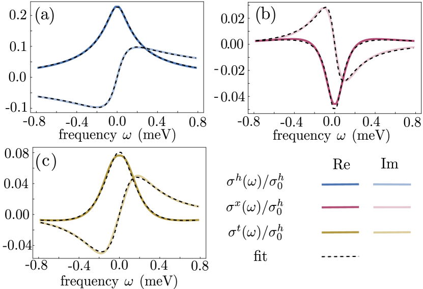
Figure 4: Ac conductivities. Ac conductivity of (a) holes, (b) excitons and (c) trions, at $\Delta/E_{F}^{h}=0.5$ and $T=5.8$ K obtained from the kinetic approach (solid lines) and fitted to the three-fluid model (dashed lines).

Ac transport properties.— Having analyzed the Feshbach tunable transport of our Bose-Fermi mixture, we now focus on the ac response, see Fig. 4. Albeit challenging to measure experimentally at this point, the ac response provides us with insights in the underlying coupled transport mechanism. We find that the ac response can be effectively described by a simple three-fluid model in terms of the hydrodynamic variables $\bm{v}_{h},\bm{v}_{x},\bm{v}_{t}$, which identify as the velocities of the fluids [41].

$$\dot{\bm{v}}_{h}-\frac{e\mathbf{E}}{m_{h}}+\frac{\bm{v}_{h}}{\tau_{h}} =-\alpha_{th}\frac{n_{t}}{m_{h}}\,(\bm{v}_{h}-\bm{v}_{t})-\alpha_{xh}\frac{n_{x}}{m_{h}}\,(\bm{v}_{h}-\bm{v}_{x}),$$

$$\dot{\bm{v}}_{x}+\frac{\bm{v}_{x}}{\tau_{x}} =-\alpha_{tx}\frac{n_{t}}{m_{x}}\,(\bm{v}_{x}-\bm{v}_{t})-\alpha_{xh}\frac{n_{h}}{m_{x}}\,\bm{(}\bm{v}_{x}-\bm{v}_{h}),$$

$$\dot{\bm{v}}_{t}+\frac{\bm{v}_{t}}{\tau_{t}} =-\alpha_{th}\frac{n_{h}}{m_{t}}\,(\bm{v}_{t}-\bm{v}_{h})-\alpha_{tx}\frac{n_{x}}{m_{t}}\,\bm{(}\bm{v}_{t}-\bm{v}_{x}),$$

where $\dot{\bm{v}}_{i}$ is the time derivative of ${\bm{v}}_{i}$. Three drag coefficients $\alpha_{ij}$, with $i\neq j\in\{h,x,t\}$, model the effect of interactions in the Bose-Fermi mixture as “viscous friction forces.” The three momentum relaxation rates $\tau_{i}$, for $i\in\{h,x,t\}$, model the many-body corrections to $\tau_{0}$. Only holes feel the longitudinal acceleration field $e\mathbf{E}/m_{h}$. The right hand side of the equations is the most general system of linear coupling terms which vanishes at $\bm{v}_{h}=\bm{v}_{x}=\bm{v}_{t}$ and preserves the total momentum $\bm{P}=\sum_{i}n_{i}m_{i}\bm{v}_{i}$ (i.e. they ensure $\dot{\bm{P}}=\bm{0}$ in the limit $\tau_{i}\rightarrow\infty$ and at $\mathbf{E}=\bm{0}$). Solving these equations, we obtain the ac conductivities from $n_{i}\bm{v}_{i}=\sigma^{i}\,\mathbf{E}/e$ as functions of six parameters $\tau_{h},\tau_{x},\tau_{t},\alpha_{xh},\alpha_{th},\alpha_{tx}$ which are functions of $\Delta$ and $T$; for instance, the sign-switching exciton drag coincides with a sign-switching drag coefficient $\alpha_{xh}\propto\text{sign}(\Delta-\Delta_{\star})$. A striking feature of the ac results is that the dissipative part of drag conductivities of excitons and trions ${\rm Re}(\sigma^{x}),{\rm Re}(\sigma^{t})$ change their sign at a finite frequency set by the competition between drag forces and relaxation rates, highlighting the deviations from the Lorentz-shaped Drude behavior.

Outlook.— In this work we consider tunable Bose-Fermi mixtures realized in TMD heterostructures. We demonstrate that a solid-state Feshbach resonance can selectively enhance exciton-hole scattering, which significantly modifies transport properties. Remarkably, we show that many-body scattering dominates over other scattering channels such as disorder and phonons, provided the system is cooled below the Bloch-Grüneisen temperature. As a result of the resonant interactions, we predict an unconventional temperature dependence of the conductivities and a sign-changing exciton drag. Our results demonstrate the potential for TMD heterostructuers to investigate strongly interacting Bose-Fermi mixtures, which appear in a variety of physical settings.

Looking forward, our results offer a promising route to study the interplay of transport and pairing instabilities in Bose-Fermi mixtures, as low relative temperatures $T/T_{F}\leq 0.01$ are already experimentally accessible [33, 32, 34, 15]. In these regimes, excitons are likely condensed, rendering phase fluctuations of the exciton gas important [9, 42, 29]. This presents a unique opportunity to explore how pairing instabilities and transport phenomena are affected by exciton condensation in strongly coupled systems. Moreover, further theoretical investigations could shed light on the hydrodynamic behavior of these quantum mixtures [43, 44, 45], which can become accessible in particularly clean heterostructures.

Acknowledgments.— We thank Z. Hao, A. Imamoğlu, and A. Mozes for fruitful discussions. We acknowledge support from the Deutsche Forschungsgemeinschaft (DFG, German Research Foundation) under Germany’s Excellence Strategy–EXC–2111–390814868, TRR 360 – 492547816 and DFG grants No. KN1254/1-2, KN1254/2-1, the European Research Council (ERC) under the European Union’s Horizon 2020 research and innovation programme (grant agreement No. 851161), as well as the Munich Quantum Valley, which is supported by the Bavarian state government with funds from the Hightech Agenda Bayern Plus. C.K. acknowledges funding from the Swiss National Science Foundation (Postdoc.Mobility Grant No. 217884).

Data availability.— Data and codes are available upon reasonable request on Zenodo [46].

Author contributions.— C.Z. and L.M. developed the kinetic theory. C.K. developed the Kubo formalism. C.Z. performed the numerical analysis. M.K. conceived the project. All authors contributed to the discussions of the results and the writing of the manuscript.

Appendix A Kinetic equations

Derivation.— Starting from the Hamiltonian Eq. (1), we derive a set of three coupled Boltzmann equations,

$$\Big{(}\partial_{t}+\mathbb{v}_{i}\cdot\bm{\partial}_{\mathbf{r}}+\mathbf{f}_{i}\cdot\bm{\partial}_{\mathbf{q}}\Big{)}F_{i} =I_{i}[F_{h},F_{x},F_{t}],$$ (5)

for the three species of particles, $i\in\{h,x,t\}$, holes, excitons, trions, respectively. These equations provide a semiclassical approximation of the dynamics of the system out of equilibrium, where $F_{i}(\mathbb{r},\mathbb{q},t)$ are the quasiparticle mass-shell distribution functions in phase space (at position $\mathbf{r}$ and momentum $\mathbf{q}$), to be determined. On the left-hand side, $\mathbf{f}_{i}(\mathbf{r},\mathbf{q})$ is the force acting on a particle and $\mathbf{v}_{i}(\mathbf{r},\mathbf{q})$ is the particle’s velocity. The right-hand side $I_{i}$ is the collision integral, which accounts for the effect of out-of-equilibrium many-body scattering as well as incoherent background scattering arising for example from impurities.

We use the real-time formalism for nonequilibrium field theory [35, 47] to obtain the hole-exciton-trion contribution to the kinetic equations Eq. (5). This involves defining the quantum action along a closed time contour going forward from $t=-\infty$ to $t=+\infty$, then backward from $t=+\infty$ to $t=-\infty$, and for each a different set of quantum fields. In coherent state notations where $\bar{x},\bar{h},\bar{t}$ represent the conjugate fields of $x,h,t$ respectively, we thus introduce $x^{\pm},\bar{x}^{\pm},h^{\pm},\bar{h}^{\pm},t^{\pm},\bar{t}^{\pm}$ where $+$ labels operators appearing in the forward-time integral, and $-$ in the backward-time integral. We recall the Keldysh rotation for a bosonic field $x$

$$x_{\rm cl/q}(t) =\big{(}x^{+}(t)\pm x^{-}(t)\big{)}/\sqrt{2},$$ (6a)

$$\bar{x}_{\rm cl/q}(t) =\big{(}\bar{x}^{+}(t)\pm\bar{x}^{-}(t)\big{)}/\sqrt{2},$$ (6b)

where $+$ is for “cl” and $-$ for “q” in $\pm$, while for a fermionic field $f$ (here $f=h,t$)

$$f_{\rm r/a}(t) =\big{(}f^{+}(t)\pm f^{-}(t)\big{)}/\sqrt{2},$$ (7a)

$$\bar{f}_{\rm r/a}(t) =\big{(}\bar{f}^{+}(t)\mp\bar{f}^{-}(t)\big{)}/\sqrt{2},$$ (7b)

where $+$ is for “r” and $-$ for “a” in the first line and conversely in the second. The action for the free fields ($f=h,t$) reads

$$S_{x,0} =\sum_{\mathbf{k},\mathbf{k}^{\prime}}\int\text{d}t\begin{bmatrix}\overline{x}^{\rm cl}\\ \overline{x}^{\rm q}\end{bmatrix}^{\top}_{\mathbf{k}}\begin{bmatrix}0&[G_{x,0}^{-1}]^{\rm A}\\ [G_{x,0}^{-1}]^{\rm R}&[G_{x,0}^{-1}]^{\rm K}\end{bmatrix}_{\mathbf{k},\mathbf{k}^{\prime}}\begin{bmatrix}x^{\rm cl}\\ x^{\rm q}\end{bmatrix}_{\mathbf{k}^{\prime}},$$ (8)

$$S_{f,0} =\sum_{\mathbf{p},\mathbf{p}^{\prime}}\int\text{d}t\begin{bmatrix}\overline{f}^{\rm r}\\ \overline{f}^{\rm a}\end{bmatrix}^{\top}_{\mathbf{p}}\begin{bmatrix}[G_{b,0}^{-1}]^{\rm R}&[G_{b,0}^{-1}]^{\rm K}\\ 0&[G_{b,0}^{-1}]^{\rm A}\end{bmatrix}_{\mathbf{p},\mathbf{p}^{\prime}}\begin{bmatrix}f^{\rm r}\\ f^{\rm a}\end{bmatrix}_{\mathbf{p}^{\prime}}.$$ (9)

Here and in the following, time integrals are defined along the forward contour.

Eqs. (8),(9) involve the free (retarded and advanced) bosonic propagator $[G_{x,0}^{\rm R/A}]_{\mathbf{k},\mathbf{k}^{\prime}}(E)=\frac{\delta_{\mathbf{k},\mathbf{k}^{\prime}}}{E-\omega_{\mathbf{k}}\pm i0^{+}}$ and fermionic propagator $[G_{f,0}^{\rm R/A}]_{\mathbf{p},\mathbf{p}^{\prime}}(E)=\frac{\delta_{\mathbf{p},\mathbf{p}^{\prime}}}{E-\epsilon_{f,\mathbf{p}}\pm i0^{+}}$, where $+$ is for “R” and $-$ is for “A” in $\pm$.

The free Keldysh propagators are for bosons $[G_{x,0}^{\rm K}]_{\mathbf{k},\mathbf{k}^{\prime}}(E)=-2i\pi F_{x}(\mathbf{k},E)\delta(E-\omega_{\mathbf{k}})\delta_{\mathbf{k},\mathbf{k}^{\prime}}$ and for fermions $[G_{f,0}^{\rm K}]_{\mathbf{p},\mathbf{p}^{\prime}}(E)=-2i\pi F_{f}(\mathbf{p},E)\delta(E-\epsilon_{f,\mathbf{p}})\delta_{\mathbf{p},\mathbf{p}^{\prime}}$; at this stage $F_{i}(\mathbf{q},E)$ are just parameter functions.

The interacting part of the action, in terms of the Keldysh-rotated fields, reads

$$S_{\rm int} =-\frac{g}{\sqrt{2N}}\int\text{d}t\sum_{\mathbf{k},\mathbf{p}}\Big{(}x_{\mathbf{k}}^{\rm cl}\,\bar{t}_{\mathbf{p}+\mathbf{k}}^{\rm a}\,h_{\mathbf{p}}^{\rm a}+x_{\mathbf{k}}^{\rm cl}\,\bar{t}_{\mathbf{p}+\mathbf{k}}^{\rm r}\,h_{\mathbf{p}}^{\rm r}$$ (10)

$$\qquad\qquad+x_{\mathbf{k}}^{\rm q}\,\bar{t}_{\mathbf{p}+\mathbf{k}}^{\rm a}\,h_{\mathbf{p}}^{\rm r}+x_{\mathbf{k}}^{\rm q}\,\bar{t}_{\mathbf{p}+\mathbf{k}}^{\rm r}\,h_{\mathbf{p}}^{\rm a}\Big{)}+\rm h.c.,$$

where “+ h.c.” means conjugating all fields (in the coherent state path integral sense), exchanging r/a and commuting the fermionic Grassmann fields. Here $N$ is the total number of unit cells in a layer, and in the following $A$ will be the total area of a layer.

From Eq. (10), the self-energies can be obtained perturbatively from Dyson’s equation,

$$\bm{G}_{i}(t,t^{\prime}) =\bm{G}_{0,i}(t-t^{\prime})$$ (11)

$$+\iint\text{d}t_{1}\text{d}t_{2}\bm{G}_{0,i}(t-t_{1})\bm{\Sigma}_{i}(t_{1},t_{2})\bm{G}_{i}(t_{2}-t^{\prime}),$$

for $i\in{h,x,t}$ and where all quantities $\bm{G}_{i},\bm{G}_{0,i},\bm{\Sigma}_{i}$ have a matrix structure in momentum space (i.e. they are functions of two momentum variables) and in Keldysh space (they have a $2\times 2$ structure with indices $\{\text{cl,q}\}$ for the bosons and $\{\text{r,a}\}$ for the fermions). The interacting theory retains the same matrix structure as the free theory, thus defining retarded, advanced and Keldysh self energies [35, 47]; for bosons $\Sigma_{x}^{\rm R}=\Sigma_{x}^{\rm q,cl}\,,\,\,\Sigma_{x}^{\rm A}=\Sigma_{x}^{\rm cl,q}\,,\,\,\Sigma_{x}^{\rm K}=\Sigma_{x}^{\rm q,q}$, and for fermions $\Sigma_{f}^{\rm R}=\Sigma_{f}^{\rm r,r}\,,\,\,\Sigma_{f}^{\rm A}=\Sigma_{f}^{\rm a,a}\,,\,\,\Sigma_{f}^{\rm K}=\Sigma_{f}^{\rm r,a}$ where $f\in\{h,t\}$.

The kinetic theory is obtained as a semiclassical approximation of the time evolution equations in phase space. This is obtained by computing the Wigner transform of the self-energy,

$$\bm{\Sigma}_{i}[\mathbf{R},t;\mathbf{k},E] =\textstyle{\int\text{d}t^{\prime}\,e^{iEt^{\prime}}\sum_{\mathbf{k}^{\prime}}}e^{i\mathbf{k}^{\prime}\mathbf{R}}$$

$$\times\bm{\Sigma}_{i}(\mathbf{k}+\tfrac{\mathbf{k}^{\prime}}{2},\mathbf{k}-\tfrac{\mathbf{k}^{\prime}}{2},t+\tfrac{t^{\prime}}{2},t-\tfrac{t^{\prime}}{2}),$$ (12)

where $\mathbf{R},t$ are the “slow” space and time variables, and $\mathbf{k},E$ are the “fast” momentum and energy variables. To the perturbative order $O(g^{2})$, we find

$$\Sigma^{\rm R/A}_{x}(\mathbf{k},E) =\frac{g^{2}}{2A}\sum_{\mathbf{p}}\frac{F_{t}(\mathbf{p}+\mathbf{k})-F_{h}(\mathbf{p})}{E-\epsilon_{t,\mathbf{p}+\mathbf{k}}+\epsilon_{h,\mathbf{p}}\pm i0},$$ (13a)

$$\Sigma^{\rm R/A}_{h}(\mathbf{p},E) =-\frac{g^{2}}{2A}\sum_{\mathbf{k}}\frac{F_{t}(\mathbf{k}+\mathbf{p})-F_{x}(\mathbf{k})}{E+\omega_{\mathbf{k}}-\epsilon_{t,\mathbf{k}+\mathbf{p}}\pm i0},$$ (13b)

$$\Sigma^{\rm R/A}_{t}(\mathbf{p},E) =\frac{g^{2}}{2A}\sum_{\mathbf{k}}\frac{F_{x}(\mathbf{k})+F_{h}(\mathbf{p}-\mathbf{k})}{E-\omega_{\mathbf{k}}-\epsilon_{h,\mathbf{p}-\mathbf{k}}\pm i0},$$ (13c)

where $+$ is for R and $-$ is for A in $\pm$, and

$$\Sigma^{\rm K}_{x}(\mathbf{k},E) =-\frac{i\pi g^{2}}{A}\sum_{\mathbf{p}}\Big{(}1-F_{t}(\mathbf{p}+\mathbf{k})F_{h}(\mathbf{p})\Big{)}\times$$

$$\times\delta\Big{(}E-\epsilon_{t,\mathbf{p}+\mathbf{k}}+\epsilon_{h,\mathbf{p}}\Big{)},$$ (14a)

$$\Sigma^{\rm K}_{h}(\mathbf{p},E) =\frac{i\pi g^{2}}{A}\sum_{\mathbf{k}}\big{(}1-F_{t}(\mathbf{k}+\mathbf{p})F_{x}(\mathbf{k})\big{)}\times$$

$$\times\delta(E+\omega_{\mathbf{k}}-\epsilon_{t,\mathbf{k}+\mathbf{p}}),$$ (14b)

$$\Sigma^{\rm K}_{t}(\mathbf{p},E) =-\frac{i\pi g^{2}}{A}\sum_{\mathbf{k}}(F_{x}(\mathbf{k})F_{h}(\mathbf{p}-\mathbf{k})+1)\times$$

$$\times\delta(E-\omega_{\mathbf{k}}-\epsilon_{\mathbf{p}-\mathbf{k}}).$$ (14c)

In Eqs. (13a)–(14c) and all the following, we keep implicit the dependence of distributions $F_{i}$ on the slow variables $\mathbf{R},t$. The collision integral is obtained from the the Wigner transform of the self-energy as

$$\tilde{I}_{i}(\mathbf{q})=i\Sigma^{\rm K}_{i}(\mathbb{q},\xi_{i,\mathbf{q}})+2{\rm Im}\Sigma^{\rm R}_{i}(\mathbb{q},\xi_{i,\mathbf{q}})F_{i}(\mathbf{q},\xi_{i,\mathbf{q}}),$$ (15)

with the shorthand $\xi_{x,\mathbf{q}}=\omega_{\mathbf{q}}$ and $\xi_{f,\mathbf{q}}=\epsilon_{f,\mathbf{q}}$. In general $F_{i}(\mathbb{q},E)$ is a function of energy and momentum independently, however in Eq. (15) the energy variable is locked to the particle dispersion: this is a semiclassical approximation which relies on the existence of well-defined quasiparticles and allows one to write simply $F_{i}(\mathbf{q})$ where the on-shell energy argument $\xi_{i,\mathbf{q}}$ is implicit.

Inserting Eqs. (13a)–(14c) into Eq. (15) gives

$$\tilde{I}_{x} =\frac{g^{2}\pi}{A}\sum_{\mathbf{p}}\delta\Big{(}\omega_{\mathbf{k}}-\epsilon_{t,\mathbf{p}+\mathbf{k}}+\epsilon_{h,\mathbf{p}}\Big{)}\bigg{[}\big{(}1-F_{t}(\mathbf{p}+\mathbf{k})\;F_{h}(\mathbf{p})\big{)}+\big{(}F_{h}(\mathbf{p})-F_{t}(\mathbf{p}+\mathbf{k})\big{)}F_{x}(\mathbf{k})\bigg{]},$$ (16a)

$$\tilde{I}_{h} =-\frac{g^{2}\pi}{A}\sum_{\mathbf{k}}\delta\Big{(}\omega_{\mathbf{k}}-\epsilon_{t,\mathbf{k}+\mathbf{p}}+\epsilon_{h,\mathbf{p}}\Big{)}\bigg{[}\big{(}1-F_{t}(\mathbf{k}+\mathbf{p})\;F_{x}(\mathbf{k})\big{)}+\big{(}F_{x}(\mathbf{k})-F_{t}(\mathbf{k}+\mathbf{p})\big{)}F_{h}(\mathbf{p})\bigg{]},$$ (16b)

$$\tilde{I}_{t} =\frac{g^{2}\pi}{A}\sum_{\mathbf{k}}\delta\Big{(}\omega_{\mathbf{k}}+\epsilon_{h,\mathbf{p}-\mathbf{k}}-\epsilon_{t,\mathbf{p}}\Big{)}\bigg{[}\big{(}1+F_{x}(\mathbf{k})\;F_{h}(\mathbf{p}-\mathbf{k})\big{)}-\big{(}F_{x}(\mathbf{k})+F_{h}(\mathbf{p}-\mathbf{k})\big{)}F_{t}(\mathbf{p})\bigg{]}.$$ (16c)

These collision integrals satisfy detailed balance: they vanish when $F_{i}$ are replaced by their equilibrium values $F_{x}^{\rm eq}(\mathbf{k})=1+2n_{\rm B}(\omega_{\mathbf{k}})$ and $F_{h}^{\rm eq}(\mathbf{p})=1-2n_{\rm F}(\epsilon_{h,\mathbf{p}})$ and $F_{t}^{\rm eq}(\mathbf{p})=1-2n_{\rm F}(\epsilon_{t,\mathbf{p}})$. Thus $\tilde{I}_{i}$ capture interaction effects out of equilibrium, however they preserve total momentum [48] and do not account for current relaxation. In other words, $\tilde{I}_{i}$ may capture drag effects but not diffusive transport. We then include momentum relaxation for all three species in the relaxation time approximation, at the rates $\tau_{h,\mathbf{p}},\tau_{x,\mathbf{k}},\tau_{t,\mathbf{p}}$. Such a collision term can arise from incoherent background scattering, for instance due to impurities. Thus, in Eq. (5) we take $I_{i}[F_{h},F_{x},F_{t}]=\tilde{I}_{i}[F_{h},F_{x},F_{t}]-(F_{i}-F_{i}^{\rm eq})/\tau_{i}$.

Besides, in Eq. (5) all the energies, velocities and quasiparticle weights are in principle renormalized by interactions. However, such corrections are always higher order in powers of $g^{2}$ or $\tau_{0}/E_{\rm F}^{h}$ than our level of approximation, thus we neglect such corrections and use the bare dispersions $\omega_{\mathbf{k}},\epsilon_{h,\mathbf{p}},\epsilon_{t,\mathbf{p}}$ and velocities $\mathbb{v}_{x}(\mathbf{k})=\partial_{\mathbb{k}}\omega(\mathbb{k})$, $\mathbb{v}_{h}(\mathbf{p})=\partial_{\mathbb{p}}\epsilon_{h}(\mathbb{p})$, $\mathbb{v}_{t}(\mathbf{k})=\partial_{\mathbf{p}}\epsilon_{t}(\mathbb{p})$. In the setup we consider, the electric field $\mathbf{E}$ applies solely to the holes, thus $\mathbf{f}_{h,\mathbf{p}}=e\mathbf{E}$ and $\mathbf{f}_{x,\mathbf{k}}=0=\mathbf{f}_{t,\mathbf{p}}=0$. We furthermore assume a homogenous system (where temperature and chemical potentials are uniform), so that all gradient terms vanish in equilibrium, $\mathbf{v}_{i}\bm{\partial}_{\mathbf{r}}F_{i}^{\rm eq}=0$.

Solution.— We proceed by linearizing the kinetic equations Eq. (5) around equilibrium. We parameterize the non-equilibrium distributions as $F_{x}(\mathbf{k})=F_{x}^{\rm eq}(\mathbf{k})+2\varphi_{x}(\mathbf{k})$ and $F_{h}(\mathbf{p})=F_{h}^{\rm eq}(\mathbf{p})-2\varphi_{h}(\mathbf{p})$ and $F_{t}(\mathbf{p})=F_{t}^{\rm eq}(\mathbf{p})-2\varphi_{t}(\mathbf{p})$ for excitons, holes and trions respectively, $n_{\rm B},n_{\rm F}$ are the Bose and Fermi functions, and $\varphi_{h},\varphi_{x},\varphi_{t}$ are the deviations from equilibrium of the particle populations. From these, the conductivities are then defined as

$$\sigma^{i}(\Omega)\mathbf{E}=e\int\frac{\text{d}^{2}\mathbb{k}}{(2\pi)^{2}}\,\,\mathbb{v}_{i}(\mathbf{k})\,\varphi_{i}(\mathbb{k})$$ (17)

for $i\in{h,x,t}$. The linear response of the system to the external electric field is obtained by performing this replacement in the collision integral, while simply replacing $F_{i}$ by $F_{i}^{\rm eq}$ on the left-hand side, except for the partial time derivative term which we write, in ac notations, as $i\Omega(F_{i}-F^{\rm eq}_{i})$. As a result, we obtain the set of three coupled algebraic equations

$$\bigg{(}\frac{1}{\tau_{x,\mathbf{k}}}+i\Omega\bigg{)}\varphi_{x}(\mathbf{k})=\frac{2\pi}{A}g^{2}\sum_{\mathbf{p}}\delta\Big{(}\omega_{\mathbf{k}}-\epsilon_{t,\mathbf{p}+\mathbf{k}}+\epsilon_{h,\mathbf{p}}\Big{)}\bigg{[}\big{(}n_{\rm F}(\epsilon_{t,\mathbf{p}+\mathbf{k}})-n_{\rm F}(\epsilon_{h,\mathbf{p}})\big{)}\varphi_{x}(\mathbf{k})$$

$$\qquad\qquad+\big{(}n_{\rm B}(\omega_{\mathbf{k}})-n_{\rm F}(\epsilon_{h,\mathbf{p}})+1\big{)}\varphi_{t}(\mathbf{p}+\mathbf{k})-\big{(}n_{\rm F}(\epsilon_{t,\mathbf{p}+\mathbf{k}})+n_{\rm B}(\omega_{\mathbf{k}})\big{)}\varphi_{h}(\mathbf{p})\bigg{]},$$ (18a)

$$\bigg{(}\frac{1}{\tau_{h,\mathbf{k}}}+i\Omega\bigg{)}\varphi_{h}(\mathbf{p})=\frac{2\pi}{A}g^{2}\sum_{\mathbf{k}}\delta\big{(}\omega_{\mathbf{k}}+\epsilon_{h,\mathbf{p}}-\epsilon_{t,\mathbf{p}+\mathbf{k}}\big{)}\bigg{[}\varphi_{x}(\mathbf{k})\big{(}n_{\rm F}(\epsilon_{t,\mathbf{k}+\mathbf{p}})-n_{\rm F}(\epsilon_{h,\mathbf{p}})\big{)}$$

$$\qquad\qquad+\varphi_{t}(\mathbf{k}+\mathbf{p})\big{(}n_{\rm B}(\omega_{\mathbf{k}})-n_{\rm F}(\epsilon_{h,\mathbf{p}})+1\big{)}-\varphi_{h}(\mathbf{p})\big{(}n_{\rm B}(\omega_{\mathbf{k}})+n_{\rm F}(\epsilon_{t,\mathbf{p}+\mathbf{k}})\big{)}\bigg{]}-\Big{(}\bm{f}_{h,\mathbf{p}}\cdot\bm{\partial}_{\mathbf{p}}\Big{)}n_{\rm F}(\epsilon_{h,\mathbf{p}}),$$ (18b)

$$\bigg{(}\frac{1}{\tau_{t,\mathbf{p}}}+i\Omega\bigg{)}\varphi_{t}(\mathbf{p})=\frac{2\pi}{A}g^{2}\sum_{\mathbf{k}}\delta\big{(}\omega_{\mathbf{k}}+\epsilon_{h,\mathbf{p}-\mathbf{k}}-\epsilon_{t,\mathbf{p}}\big{)}\bigg{[}\varphi_{x}(\mathbf{k})\big{(}n_{\rm F}(\epsilon_{h,\mathbf{p}-\mathbf{k}})-n_{\rm F}(\epsilon_{t,\mathbf{p}})\big{)}$$

$$\qquad\qquad-\varphi_{t}(\mathbf{p})\big{(}n_{\rm B}(\omega_{\mathbf{k}})-n_{\rm F}(\epsilon_{h,\mathbf{p}-\mathbf{k}})+1\big{)}+\varphi_{h}(\mathbf{p}-\mathbf{k})\big{(}n_{\rm B}(\omega_{\mathbf{k}})+n_{\rm F}(\epsilon_{t,\mathbf{p}})\big{)}\bigg{]}.$$ (18c)

In what follows, we use matrix notations for objects that are function of two momenta. In particular, we define the vector $\mathcal{K}^{h}_{\mathbf{p}}=\Big{(}\mathbf{f}_{h,\mathbf{p}}\cdot\bm{\partial}_{\mathbf{p}}\Big{)}\,n_{\rm F}(\epsilon_{h,\mathbf{p}})$ and the diagonal matrices $\Upsilon^{i}_{\mathbf{q},\mathbf{q}^{\prime}}=\delta_{\mathbf{q},\mathbf{q}^{\prime}}\bigg{(}\frac{1}{\tau_{i,\mathbf{q}}}+i\Omega\bigg{)}$ and

$$\mathcal{M}^{t}_{\mathbb{p},\mathbb{q}}=\delta_{\mathbb{q},\mathbb{p}}\frac{2\pi}{A}g^{2}\sum_{\mathbf{k}}\delta\big{(}\omega_{\mathbf{k}}+\epsilon_{h,\mathbf{p}-\mathbf{k}}-\epsilon_{t,\mathbf{p}}\big{)}\;\Big{(}n_{\rm B}(\omega_{\mathbf{k}})+1-n_{\rm F}(\epsilon_{h,\mathbf{p}-\mathbf{k}})\Big{)}.$$ (19)

We first solve for $\varphi_{t}(\mathbf{p})$ in terms of $\varphi_{x}(\mathbf{k}),\varphi_{h}(\mathbf{p})$:

$$\varphi_{t}(\mathbb{p}) =\frac{2\pi}{A}g^{2}\sum_{\mathbf{k}}\left(\mathcal{M}^{t}+\Upsilon_{t}\right)^{-1}_{\mathbb{p},\mathbb{p}}\delta\Big{(}\omega_{\mathbf{k}}+\epsilon_{h,\mathbf{p}-\mathbf{k}}-\epsilon_{t,\mathbf{p}}\Big{)}$$

$$\qquad\qquad\times\bigg{(}(n_{F}(\epsilon_{h,\mathbb{p}-\mathbb{k}})-n_{F}(\epsilon_{t,\mathbb{p}}))\,\varphi_{x}(\mathbb{k})+(n_{B}(\omega_{\mathbb{k}})+n_{F}(\epsilon_{t,\mathbb{p}}))\,\varphi_{h}(\mathbb{p}-\mathbb{k})\bigg{)},$$ (20)

By substituting Eq. (A) back into Eqs. (18), we find the following expression for $\varphi_{x}$ and $\varphi_{h}$:

$$\varphi_{h}(\mathbb{p}) =-\bigg{[}\mathcal{M}^{h}+\Upsilon^{h}-\mathcal{N}^{h}\Big{(}\mathcal{M}^{x}+\Upsilon^{x}\Big{)}^{-1}\mathcal{N}^{x}\bigg{]}^{-1}_{\mathbb{p},\mathbb{q}}\mathcal{K}^{h}_{\mathbb{q}},$$ (21)

$$\varphi_{x}(\mathbb{k}) =\bigg{[}\mathcal{M}^{x}+\Upsilon^{x}-\mathcal{N}^{x}\Big{(}\mathcal{M}^{h}+\Upsilon^{h}\Big{)}^{-1}\mathcal{N}^{h}\bigg{]}^{-1}_{\mathbb{k},\mathbb{q}}\,\bigg{(}\mathcal{N}_{x}\Big{(}\mathcal{M}_{h}+\Upsilon_{h}\Big{)}^{-1}\mathcal{K}^{h}\bigg{)}_{\mathbb{q}},$$ (22)

where repeated indices imply implicit summation, and for brevity we defined the following matrices:

$$\mathcal{M}^{x}_{\mathbf{k},\mathbf{q}} =\delta_{\mathbf{k},\mathbf{q}}\frac{2\pi}{A}g^{2}\sum_{\mathbf{p}}\delta(\omega_{\mathbf{k}}-\epsilon_{t,\mathbf{p}+\mathbf{k}}+\epsilon_{h,\mathbf{p}})\left(n_{F}(\epsilon_{h,\mathbf{p}})-n_{F}(\epsilon_{t,\mathbf{k}+\mathbf{p}})\right)-\frac{4\pi^{2}}{A^{2}}g^{4}\sum_{\mathbf{p}}\delta(\omega_{\mathbf{k}}-\epsilon_{t,\mathbf{p}+\mathbf{k}}+\epsilon_{h,\mathbf{p}})\mathcal{Q}^{x}_{\mathbf{q},\mathbf{p},\mathbf{k}},$$ (23a)

$$\mathcal{N}^{x}_{\mathbf{k},\mathbf{q}} =\frac{2\pi}{A}g^{2}\delta(\omega_{\mathbf{k}}-\epsilon_{t,\mathbf{q}+\mathbf{k}}+\epsilon_{h,\mathbf{q}})\big{(}n_{F}(\epsilon_{t,\mathbf{q}+\mathbf{k}})+n_{B}(\omega_{\mathbf{k}})\big{)}-\frac{4\pi^{2}}{A^{2}}g^{4}\sum_{\mathbf{p}}\delta(\omega_{\mathbf{k}}-\epsilon_{t,\mathbf{p}+\mathbf{k}}+\epsilon_{h,\mathbf{p}})\mathcal{Q}^{h}_{\mathbf{q},\mathbf{p},\mathbf{k}},$$ (23b)

$$\mathcal{M}^{h}_{\mathbf{p},\mathbf{q}} =\delta_{\mathbf{p},\mathbf{q}}\frac{2\pi}{A}g^{2}\sum_{\mathbf{k}}\delta(\omega_{\mathbf{k}}+\epsilon_{h,\mathbf{p}}-\epsilon_{t,\mathbf{p}+\mathbf{k}})\left(n_{F}(\epsilon_{t,\mathbf{p}+\mathbf{k}})+n_{B}(\omega_{\mathbf{k}})\right)-\frac{4\pi^{2}}{A^{2}}g^{4}\sum_{\mathbf{k}}\delta(\omega_{\mathbf{k}}+\epsilon_{h,\mathbf{p}}-\epsilon_{t,\mathbf{p}+\mathbf{k}})\mathcal{Q}^{h}_{\mathbf{q},\mathbf{p},\mathbf{k}},$$ (23c)

$$\mathcal{N}^{h}_{\mathbf{p},\mathbf{q}} =\frac{2\pi}{A}g^{2}\delta(\omega_{\mathbf{q}}+\epsilon_{h,\mathbf{p}}-\epsilon_{t,\mathbf{p}+\mathbf{q}})\big{(}n_{F}(\epsilon_{h,\mathbf{p}})-n_{F}(\epsilon_{t,\mathbf{p}+\mathbf{q}})\big{)}-\frac{4\pi^{2}}{A^{2}}g^{4}\sum_{\mathbf{k}}\delta(\omega_{\mathbf{k}}-\epsilon_{t,\mathbf{p}+\mathbf{k}}+\epsilon_{h,\mathbf{p}})\mathcal{Q}^{x}_{\mathbf{q},\mathbf{p},\mathbf{k}},$$ (23d)

$$\mathcal{Q}^{x}_{\mathbf{q},\mathbf{p},\mathbf{k}} =(\Upsilon^{t}+\mathcal{M}^{t})^{-1}_{\mathbf{p}+\mathbf{k},\mathbf{p}+\mathbf{k}}(1+n_{B}(\omega_{\mathbf{k}})-n_{F}(\epsilon_{h,\mathbf{p}}))\delta(\omega_{\mathbf{q}}+\epsilon_{h,\mathbf{p}+\mathbf{k}-\mathbf{q}}-\epsilon_{t,\mathbf{p}+\mathbf{k}})\big{(}n_{F}(\epsilon_{h,\mathbf{p}+\mathbf{k}-\mathbf{q}})-n_{F}(\epsilon_{t,\mathbf{p}+\mathbf{k}})\big{)},$$ (24a)

$$\mathcal{Q}^{h}_{\mathbf{q},\mathbf{p},\mathbf{k}} =(\Upsilon^{t}+\mathcal{M}^{t})^{-1}_{\mathbf{p}+\mathbf{k},\mathbf{p}+\mathbf{k}}(1+n_{B}(\omega_{\mathbf{k}})-n_{F}(\epsilon_{h,\mathbf{p}}))\delta(\omega_{\mathbf{k}+\mathbf{p}-\mathbf{q}}+\epsilon_{h,\mathbf{q}}-\epsilon_{t,\mathbf{p}+\mathbf{k}})(n_{B}(\omega_{\mathbf{k}+\mathbf{p}-\mathbf{q}})+n_{F}(\epsilon_{t,\mathbf{p}+\mathbf{k}})).$$ (24b)

In Eqs. (23) we keep corrections which, although formally of order $O(g^{4})$, may become relevant close to resonance – see discussion in the next section.

We then obtain the conductivities Eq. (17) by a numerical evaluation of Eqs. (A)–(22) and their building blocks Eqs. (23),(24), with the choice $\tau_{i,\mathbf{q}}=\tau_{0}$ for all $i\in\{h,x,t\}$.

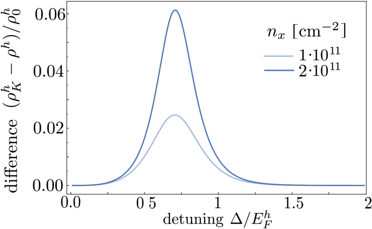
Figure 5: Comparison of Kubo and Boltzmann approaches for the hole resistivity. Difference of the hole resistivities as a function of the detuning $\Delta$ as obtained from Kubo’s formula to leading order, $\rho^{h}_{K}$, and Boltzmann’s equations as described in the previous appendix, $\rho^{h}$, for $t=1$ meV, $T=5.8$ K and for different values of the exciton density $n_{x}$. The relative difference arising from the $\mathcal{O}(g^{4})$ corrections included in the kinetic theory treatment, is of a few percent of the background resistivity $\rho_{0}^{h}$.

Appendix B Linear response from Kubo’s formula

Since the system hosts a small parameter, we can also analyze the conductivity by evaluating Kubo’s formula

$$\sigma^{h}_{ab}(\mathbf{q},\omega)=\frac{ie^{2}}{\omega}\left[\chi^{R}_{\mathbf{j}_{a}\mathbf{j}_{b}}(\mathbf{q},\omega)+\delta_{ab}\frac{\langle n_{h}\rangle}{m_{h}}\right],$$ (25)

where $\chi^{R}_{\mathbf{j}_{a}\mathbf{j}_{b}}(\mathbf{q},\omega)$ is the retarded current-current response function, $n_{h}$ is the hole density, and $a,b\in\{x,y\}$. To lowest order in $g$, the diagrammatic expression for $\chi^{R}_{\mathbf{j}_{a}\mathbf{j}_{b}}(\mathbf{q},\omega)$ yields currentcurrent

$$\chi_{\mathbf{j}_{a}\mathbf{j}_{b}}^{R}(\mathbf{q},\omega)=\begin{gathered}\fmfgraph(70,15)\fmfleft{i}\fmfright{o}\fmf{phantom}{i,v1,v2,o}\fmf{dashes,fore=(0.1,,0.1,,0.1)}{i,v1}\fmf{dashes}{v2,o}\fmffreeze\fmf{fermion,fore=(0.15,,0.2,,0.4),width=1.8,tension=1,left=0.7}{v2,v1}\fmf{fermion,fore=(0.15,,0.2,,0.4),width=1.8,left=0.7}{v1,v2}\fmfdot{v1,v2}\end{gathered}+\mathcal{O}(g^{4}),$$

where the thick blue lines denote hole propagators, which are obtained by solving Dyson’s equation to order $\mathcal{O}(g^{2})$: selfeng

$$\begin{gathered}\fmfgraph*(30,25)\fmfleft{i}\fmfright{o}\fmf{fermion,fore=(0.15,,0.2,,0.4),width=1.8}{i,o}\end{gathered}=\begin{gathered}\fmfgraph*(30,20)\fmfleft{i}\fmfright{o}\fmf{fermion,fore=(0.3,,0.4,,0.8)}{i,o}\end{gathered}+\begin{gathered}\fmfgraph(80,15)\fmfleft{i}\fmfright{o}\fmf{phantom}{i,v1,v3,o}\fmf{fermion,fore=(0.3,,0.4,,0.8),tension=5.}{i,v1}\fmf{fermion,fore=(0.15,,0.2,,0.4),tension=5,width=1.8}{v3,o}\fmf{boson,tension=1}{v3,v1}\fmf{phantom_{a}rrow}{v3,v1}\fmf{dbl_{p}lain_{a}rrow,fore=(0.9,,0.3,,0.4),left=0.75}{v1,v3}\end{gathered}.$$ (29)

In Eq. (29), light-blue, red and squiggly lines denote bare-hole, trion and exciton propagators:

$$\fmffile{propagators}\begin{aligned} \begin{gathered}\fmfgraph*(30,20)\fmfleft{i}\fmfright{o}\fmf{fermion,fore=(0.3,,0.4,,0.8)}{i,o}\end{gathered}&=\frac{1}{\omega-\xi^{h}(\mathbf{p})+i/2\tau^{0}_{h,\mathbf{q}}}\\ \begin{gathered}\fmfgraph*(30,20)\fmfleft{i}\fmfright{o}\fmf{dbl_{p}lain_{a}rrow,fore=(0.9,,0.3,,0.4)}{i,o}\end{gathered}&=\frac{1}{\omega-\xi^{t}(\mathbf{p})+i/2\tau^{0}_{t,\mathbf{q}}}\\ \begin{gathered}\fmfgraph*(30,20)\fmfleft{i}\fmfright{o}\fmf{boson}{i,o}\fmf{phantom_{a}rrow}{i,o}\end{gathered}&=\frac{1}{\omega-\omega(\mathbf{k})+i/2\tau^{0}_{x,\mathbf{q}}},\end{aligned}$$ (30)

where we have modelled background scattering by adding a finite line broadening $1/2\tau_{i,\mathbf{q}}=1/2\tau_{0}$. Evaluating these diagrams and neglecting vertex corrections, one obtains the standard result

$$\lim_{\omega\rightarrow 0}\frac{1}{\omega}\left(\chi_{\mathbf{j}_{x}\mathbf{j}_{x}}^{R}(0,\omega)+\frac{\langle n_{h}\rangle}{m_{h}}\right)$$ (31)

$$\qquad=\frac{i}{4\pi}\int_{0}^{\infty}\!\!\!dEE\int\frac{dz}{2\pi}\frac{\mathcal{A}(k(E),z)}{\rm{Im}\Sigma^{R}_{h}(k(E),z)}n_{F}^{\prime}(z),$$

where $k(E)^{2}=2m_{h}E$. The current-current response function can be expressed directly in terms of the hole spectral function

$$\mathcal{A}(\mathbf{k},z)=-2\rm{Im}G^{R}(\mathbf{k},z)$$ (32)

and their perturbatively evaluated self energy

$$\Sigma^{R}_{h}(\mathbf{k},\omega) =-g^{2}\int\frac{d^{2}\mathbf{q}}{(2\pi)^{2}}\frac{n_{F}(\epsilon_{t,\mathbf{q+k}})+n_{B}(\omega_{\mathbf{q}})}{\epsilon_{t,\mathbf{q+k}}-i/2\tau_{t,\mathbf{q+k}}-\omega-\omega_{\mathbf{q}}-i/2\tau_{x,\mathbf{q}}}-\frac{i}{2\tau_{h,\mathbf{k}}}+\mathcal{O}(g^{4});$$ (33)

see Eq. (29). By combining Eq. (25) and Eq. (31), we can express the conductivity in a standard form

$$\sigma^{h}_{xx}(\omega=0)\frac{h}{e^{2}}=\int_{-\mu}^{\infty}\!\!\!d\xi\left(\xi+\mu\right)n_{F}^{\prime}(\xi)\tau_{\mathrm{tot}}(\xi),$$ (34)

where $\tau_{\mathrm{tot}}^{-1}(\xi)=-2\rm{Im}\Sigma^{R}_{h}(k(\xi+\mu),\xi)$.

The linear response result Eq. (34) coincides with that obtained by the kinetic method in the previous subsection, to the leading order $\mathcal{O}(g^{2})$. Indeed, the term of order $g^{2}$ in $\mathcal{M}^{h}$ in Eq. (23c), responsible for the most relevant many-body contribution to the hole resistivity, is identical to $2\rm{Im}\Sigma^{R}_{h}(\mathbf{p},\epsilon_{\mathbf{p},h})$ in Eq. (33) in the limit $1/2\tau_{i,\mathbf{q}}\rightarrow 0^{+}$. The Boltzmann approach also takes into account higher orders in $g^{2}$, however we checked numerically that $\mathcal{O}(g^{4})$ corrections to the hole resistivity, albeit finite, are small for the considered parameters, see Fig. 5.

On the kinetic theory side, such formally $\mathcal{O}(g^{4})$ corrections arise from the rightmost terms in Eqs. (23), and especially in the hole resistivity case from $Q(\mathbf{p},\mathbf{q})\equiv-\frac{4\pi^{2}}{A^{2}}g^{4}\sum_{\mathbf{k}}\delta(\omega_{\mathbf{k}}+\epsilon_{h,\mathbf{p}}-\epsilon_{t,\mathbf{p}+\mathbf{k}})\mathcal{Q}^{h}_{\mathbf{q},\mathbf{p},\mathbf{k}}$ in Eq. (23c). This correction becomes relevant for $\mathbf{p}\approx\mathbf{q}$ at small temperatures $k_{B}T\ll\hbar^{2}n_{x}/m_{x}$, where the population of excitons at small momenta $\mathbb{k}\approx\bm{0}$ is a sizeable fraction of $n_{x}$. In this regime, for small values of disorder, it can be that $\Upsilon^{t}+\mathcal{M}^{t}$ is dominated by $\mathcal{M}^{t}\propto g^{2}n_{x}$. This in turn implies that $Q(\mathbf{q},\mathbf{q})\sim g^{2}n_{x}$, in contrast to its formal magnitude $\mathcal{O}(g^{4})$. This provides a relevant contribution to the hole resistivity obtained from the kinetic theory method, which in the formalism of Kubo’s equation would correspond to higher-order diagrammatic corrections to the bare conductivity bubble calculated in Eq. (31).

Appendix C Trions

The trions exhibit a drag effect similarly to the excitons. The resulting rion conductivity depends strongly on resonant interactions, see Fig. 6. For small values of the interaction parameter $g\propto\rm t$ and small temperature, $\sigma^{t}$ reaches a maximum in the vicinity of the resonance $(\Delta\approx\Delta_{\star})$ and increases with increasing $g$, as expected from the general discussion of hole-exciton-trion scattering given in the main text. At larger $g$, where $\mathcal{M}_{i}\gtrsim\Upsilon_{i}$ for $i\in\{h,x,t\}$, many-body corrections to the relaxation times become important. As a result, with increasing $g$, $\sigma^{h}$ decreases, $\sigma^{x}$ saturates, and $\sigma^{t}$ decreases before it saturates. Such corrections at large $g$ also entail less evident signatures nearby resonance, especially noticeable in the trion case. Remarkably, we find that the trion conductivity takes values of the same order of magnitude as the exciton conductivity. Therefore, the individual conductivities can be resolved by separately measuring charge currents in both the middle and the lower layer.

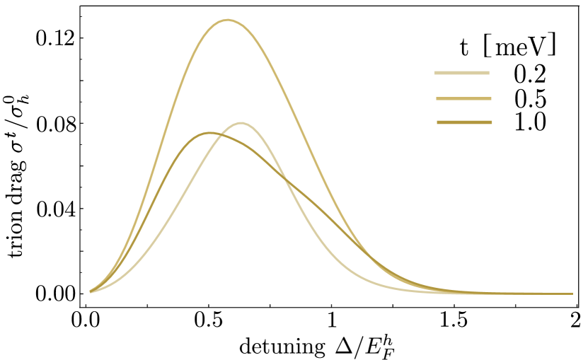
Figure 6: Trion drag across resonance. Trion conductivity as a function of the detuning $\Delta$, for $T=5.8$ K and different values of the tunneling parameter t.

Appendix D Hydrodynamic model for ac conductivities

The three-fluid model of the main text can be solved analytically. The ac conductivities of the three particle species are obtained as:

$$\sigma^{i}(\Omega) =\frac{{\sf A}_{i}}{1/\tau_{i}+i\Omega+{\sf B}_{i}}\frac{n_{i}}{n_{h}}\sigma^{h}(\Omega),$$ (35)

$$\sigma^{h}(\Omega) =\frac{e^{2}n_{h}/m_{h}}{1/\tau_{h}+i\Omega+\sum_{i=x,t}{\sf C}_{i}(1-\frac{{\sf A}_{i}}{i\Omega+1/\tau_{i}+{\sf B}_{i}})},$$ (36)

where we defined

$${\sf A}_{i}=\alpha_{ih}\frac{n_{h}}{m_{i}}+\frac{\alpha_{\overline{i}h}\alpha_{tx}n_{\overline{i}}n_{h}/m_{i}}{\alpha_{\overline{i}h}n_{h}+\alpha_{tx}n_{i}+i\Omega+1/\tau_{\overline{i}}},$$ (37a)

$${\sf B}_{i}=\frac{\alpha_{tx}n_{\overline{i}}}{m_{i}}+\frac{\alpha_{ih}n_{h}}{m_{i}}-\frac{\alpha_{tx}^{2}n_{x}n_{t}/m_{i}}{\alpha_{\overline{i}h}n_{h}+\alpha_{tx}n_{i}+i\Omega+1/\tau_{\overline{i}}},$$ (37b)

$${\sf C}_{i}=\alpha_{ih}n_{i}/m_{h}$$ (37c)

and use the shorthand notation $i=x,t\leftrightarrow\overline{i}=t,x$ respectively.

We use Eqs. (35),(36) to fit the ac conductivities, obtained by solving the system of coupled Boltzmann’s equations as described in the first appendix, reported in the main text. We find the following values for the fitting parameters: $\tau_{h}=9.4$ ps, $\tau_{x}=10.0$ ps, $\tau_{t}=2.9$ ps, $\alpha_{th}=0.64\frac{m_{0}}{n_{0}\tau_{0}}$, $\alpha_{xh}=-0.48\frac{m_{0}}{n_{0}\tau_{0}}$, $\alpha_{tx}=0.50\frac{m_{0}}{n_{0}\tau_{0}}$, where $n_{0}=10^{12}\text{cm}^{-2}$, $m_{0}=0.25m_{\sf e}$, and $\tau_{0}=10$ ps.

References

• Landau [1933] L. D. Landau, Über die bewegung der elektronen in kristallgitter, Phys. Z. Sowjetunion 3, 134512 (1933).
• Pekar [1946] S. Pekar, Autolocalization of the electron in an inertially polarizable dielectric medium, Zh. Eksp. Teor. Fiz 16, 335 (1946).
• Hertz [1976] J. A. Hertz, Quantum critical phenomena, Physical Review B 14, 1165–1184 (1976).
• Lee et al. [2006] P. A. Lee, N. Nagaosa, and X.-G. Wen, Doping a mott insulator: Physics of high-temperature superconductivity, Reviews of Modern Physics 78, 17–85 (2006).
• Löhneysen et al. [2007] H. v. Löhneysen, A. Rosch, M. Vojta, and P. Wölfle, Fermi-liquid instabilities at magnetic quantum phase transitions, Reviews of Modern Physics 79, 1015–1075 (2007).
• Sachdev [2011] S. Sachdev, Quantum Phase Transitions (Cambridge University Press, 2011).
• Li et al. [2021] T. Li, S. Jiang, L. Li, Y. Zhang, K. Kang, J. Zhu, K. Watanabe, T. Taniguchi, D. Chowdhury, L. Fu, J. Shan, and K. F. Mak, Continuous mott transition in semiconductor moiré superlattices, Nature 597, 350–354 (2021).
• Senthil [2008] T. Senthil, Theory of a continuous mott transition in two dimensions, Phys. Rev. B 78, 045109 (2008).
• Ma et al. [2021] L. Ma, P. X. Nguyen, Z. Wang, Y. Zeng, K. Watanabe, T. Taniguchi, A. H. MacDonald, K. F. Mak, and J. Shan, Strongly correlated excitonic insulator in atomic double layers, Nature 598, 585 (2021).
• Schwartz et al. [2021] I. Schwartz, Y. Shimazaki, C. Kuhlenkamp, K. Watanabe, T. Taniguchi, M. Kroner, and A. Imamoğlu, Electrically tunable feshbach resonances in twisted bilayer semiconductors, Science 374, 336–340 (2021).
• Park et al. [2023] H. Park, J. Zhu, X. Wang, Y. Wang, W. Holtzmann, T. Taniguchi, K. Watanabe, J. Yan, L. Fu, T. Cao, D. Xiao, D. R. Gamelin, H. Yu, W. Yao, and X. Xu, Dipole ladders with large Hubbard interaction in a moiré exciton lattice, Nat. Phys. 19, 1286 (2023).
• Xiong et al. [2023] R. Xiong, J. H. Nie, S. L. Brantly, P. Hays, R. Sailus, K. Watanabe, T. Taniguchi, S. Tongay, and C. Jin, Correlated insulator of excitons in WSe2/WS2 moiré superlattices, Science 380, 860 (2023).
• Gao et al. [2024] B. Gao, D. G. Suárez-Forero, S. Sarkar, T.-S. Huang, D. Session, M. J. Mehrabad, R. Ni, M. Xie, P. Upadhyay, J. Vannucci, S. Mittal, K. Watanabe, T. Taniguchi, A. Imamoglu, Y. Zhou, and M. Hafezi, Excitonic Mott insulator in a Bose-Fermi-Hubbard system of moiré WS2/WSe2 heterobilayer, Nat. Commun. 15, 1 (2024).
• Lian et al. [2024] Z. Lian, Y. Meng, L. Ma, I. Maity, L. Yan, Q. Wu, X. Huang, D. Chen, X. Chen, X. Chen, M. Blei, T. Taniguchi, K. Watanabe, S. Tongay, J. Lischner, Y.-T. Cui, and S.-F. Shi, Valley-polarized excitonic Mott insulator in WS2/WSe2 moiré superlattice, Nat. Phys. 20, 34 (2024).
• Nguyen et al. [2023] P. X. Nguyen, R. Chaturvedi, L. Ma, P. Knuppel, K. Watanabe, T. Taniguchi, K. F. Mak, and J. Shan, A degenerate trion liquid in atomic double layers (2023), arXiv:2312.12571 [cond-mat.mes-hall] .
• Qi et al. [2023] R. Qi, Q. Li, Z. Zhang, S. Chen, J. Xie, Y. Ou, Z. Cui, D. D. Dai, A. Y. Joe, T. Taniguchi, K. Watanabe, S. Tongay, A. Zettl, L. Fu, and F. Wang, Electrically controlled interlayer trion fluid in electron-hole bilayers (2023), arXiv:2312.03251 [cond-mat.mes-hall] .
• Chin et al. [2010] C. Chin, R. Grimm, P. Julienne, and E. Tiesinga, Feshbach resonances in ultracold gases, Rev. Mod. Phys. 82, 1225 (2010).
• Bloch et al. [2008] I. Bloch, J. Dalibard, and W. Zwerger, Many-body physics with ultracold gases, Rev. Mod. Phys. 80, 885 (2008).
• Ferrier-Barbut et al. [2014] I. Ferrier-Barbut, M. Delehaye, S. Laurent, A. T. Grier, M. Pierce, B. S. Rem, F. Chevy, and C. Salomon, A mixture of bose and fermi superfluids, Science 345, 1035 (2014).
• DeSalvo et al. [2019] B. J. DeSalvo, K. Patel, G. Cai, and C. Chin, Observation of fermion-mediated interactions between bosonic atoms, Nature 568, 61 (2019).
• Yan et al. [2024] Z. Z. Yan, Y. Ni, A. Chuang, P. E. Dolgirev, K. Seetharam, E. Demler, C. Robens, and M. Zwierlein, Collective flow of fermionic impurities immersed in a bose–einstein condensate, Nature Physics 20, 1395–1400 (2024).
• Duda et al. [2023] M. Duda, X.-Y. Chen, A. Schindewolf, R. Bause, J. von Milczewski, R. Schmidt, I. Bloch, and X.-Y. Luo, Transition from a polaronic condensate to a degenerate fermi gas of heteronuclear molecules, Nature Physics 19, 720 (2023).
• Wilson et al. [2021] N. P. Wilson, W. Yao, J. Shan, and X. Xu, Excitons and emergent quantum phenomena in stacked 2d semiconductors, Nature 599, 383 (2021).
• Sidler et al. [2017] M. Sidler, P. Back, O. Cotlet, A. Srivastava, T. Fink, M. Kroner, E. Demler, and A. Imamoglu, Fermi polaron-polaritons in charge-tunable atomically thin semiconductors, Nature Physics 13, 255 (2017).
• Fey et al. [2020] C. Fey, P. Schmelcher, A. Imamoglu, and R. Schmidt, Theory of exciton-electron scattering in atomically thin semiconductors, Phys. Rev. B 101, 195417 (2020).
• Kuhlenkamp et al. [2022] C. Kuhlenkamp, M. Knap, M. Wagner, R. Schmidt, and A. Imamoğlu, Tunable feshbach resonances and their spectral signatures in bilayer semiconductors, Phys. Rev. Lett. 129, 037401 (2022).
• Wagner et al. [2023] M. Wagner, R. Ołdziejewski, F. Rose, V. Köder, C. Kuhlenkamp, A. İmamoğlu, and R. Schmidt, Feshbach resonances of composite charge carrier states in atomically thin semiconductor heterostructures, arXiv:2310.08729  (2023).
• Powell et al. [2005] S. Powell, S. Sachdev, and H. P. Büchler, Depletion of the bose-einstein condensate in bose-fermi mixtures, Phys. Rev. B 72, 024534 (2005).
• Zerba et al. [2024a] C. Zerba, C. Kuhlenkamp, A. Imamoğlu, and M. Knap, Realizing topological superconductivity in tunable bose-fermi mixtures with transition metal dichalcogenide heterostructures, Phys. Rev. Lett. 133, 056902 (2024a).
• Kormányos et al. [2015] A. Kormányos, G. Burkard, M. Gmitra, J. Fabian, V. Zólyomi, N. D. Drummond, and V. Fal’ko, k·p theory for two-dimensional transition metal dichalcogenide semiconductors, 2D Materials 2, 022001 (2015).
• Jauregui et al. [2019] L. A. Jauregui, A. Y. Joe, K. Pistunova, D. S. Wild, A. A. High, Y. Zhou, G. Scuri, K. De Greve, A. Sushko, C.-H. Yu, T. Taniguchi, K. Watanabe, D. J. Needleman, M. D. Lukin, H. Park, and P. Kim, Electrical control of interlayer exciton dynamics in atomically thin heterostructures, Science 366, 870 (2019).
• Joe et al. [2024] A. Y. Joe, K. Pistunova, K. Kaasbjerg, K. Wang, B. Kim, D. A. Rhodes, T. Taniguchi, K. Watanabe, J. Hone, T. Low, L. A. Jauregui, and P. Kim, Transport study of charge-carrier scattering in monolayer ${\mathrm{wse}}_{2}$Phys. Rev. Lett. 132, 056303 (2024).
• Pack et al. [2024] J. Pack, Y. Guo, Z. Liu, B. S. Jessen, L. Holtzman, S. Liu, M. Cothrine, K. Watanabe, T. Taniguchi, D. G. Mandrus, K. Barmak, J. Hone, and C. R. Dean, Charge-transfer contacts for the measurement of correlated states in high-mobility WSe2, Nat. Nanotechnol. 19, 948 (2024).
• Guo et al. [2024] Y. Guo, J. Pack, J. Swann, L. Holtzman, M. Cothrine, K. Watanabe, T. Taniguchi, D. Mandrus, K. Barmak, J. Hone, A. J. Millis, A. N. Pasupathy, and C. R. Dean, Superconductivity in twisted bilayer wse2arXiv:2406.03418  (2024).
• Kamenev [2011] A. Kamenev, Field Theory of Non-Equilibrium Systems (Cambridge University Press, Cambridge, England, UK, 2011).
• [36] G. D. Mahan, Many-Particle Physics (Springer US).
• [37] See Supplemental Material.
• Cotleţ et al. [2019] O. Cotleţ, F. Pientka, R. Schmidt, G. Zarand, E. Demler, and A. Imamoglu, Transport of neutral optical excitations using electric fields, Phys. Rev. X 9, 041019 (2019).
• Lavasani et al. [2019] A. Lavasani, D. Bulmash, and S. Das Sarma, Wiedemann-franz law and fermi liquids, Phys. Rev. B 99, 085104 (2019).
• Huang and Das Sarma [2024] Y. Huang and S. Das Sarma, Electronic transport, metal-insulator transition, and wigner crystallization in transition metal dichalcogenide monolayers, Phys. Rev. B 109, 245431 (2024).
• [41] Formally, they are defined, for $i\in\{h,x,t\}$, by $\bm{v}_{i}(\mathbf{r})=\int\tfrac{\text{d}^{2}\mathbf{q}}{(2\pi)^{2}}\frac{\mathbf{q}}{m_{i}}f_{i}(\mathbf{r},\mathbf{q})/n_{i}(\mathbf{r})$ where $f_{i}$ is the quasi-particle distribution function in phase space and $n_{i}=\int\tfrac{\text{d}^{2}\mathbf{q}}{(2\pi)^{2}}f_{i}$.
• Cotleţ et al. [2016] O. Cotleţ, S. Zeytinoǧlu, M. Sigrist, E. Demler, and A. m. c. Imamoǧlu, Superconductivity and other collective phenomena in a hybrid bose-fermi mixture formed by a polariton condensate and an electron system in two dimensions, Phys. Rev. B 93, 054510 (2016).
• Levchenko and Schmalian [2020] A. Levchenko and J. Schmalian, Transport properties of strongly coupled electron–phonon liquids, Annals of Physics 419, 168218 (2020).
• Huang and Lucas [2021] X. Huang and A. Lucas, Electron-phonon hydrodynamics, Phys. Rev. B 103, 155128 (2021).
• Fritz and Scaffidi [2024] L. Fritz and T. Scaffidi, Hydrodynamic electronic transport, Annual Review of Condensed Matter Physics 15, 17 (2024).
• Zerba et al. [2024b] C. Zerba, C. Kuhlenkamp, L. Mangeolle, and M. Knap, Tuning transport in solid-state Bose-Fermi mixtures by Feshbach resonances (2024b).
• Rammer [2019] J. Rammer, Quantum Transport Theory (Taylor & Francis, Andover, England, UK, 2019).
• Baym and Kadanoff [1961] G. Baym and L. P. Kadanoff, Conservation laws and correlation functions, Physical Review 124, 287–299 (1961).