The $L^{1}$-relaxed area of the graph of the vortex map: optimal upper bound

Abstract

We compute an upper bound for the value of the $L^{1}$-relaxed area of the graph of the vortex map $u:{\rm B}_{l}(0)\subset\mathbb{R}^{2}\to\mathbb{R}^{2}$, $u(x):=x/|x|$, $x\neq 0$, for all values of $l>0$. Together with a previously proven lower bound, this upper bound turns out to be optimal. Interestingly, for the radius $l$ in a certain range, in particular $l$ not too large, a Plateau-type problem, having as solution a sort of catenoid constrained to contain a segment, has to be solved.

Key words:  Area functional, minimal surfaces, Plateau problem, relaxation, Cartesian currents.

AMS (MOS) subject classification: 49Q15, 49Q20, 49J45, 58E12.

1 Introduction

Determining the domain and the expression of the relaxed area functional of graphs of nonsmooth maps in codimension greater than $1$ is a challenging problem whose solution is far from being reached. Let $\Omega\subset\mathbb{R}^{n}$ be a bounded open set and let $v:\Omega\rightarrow\mathbb{R}^{N}$ be a map of class $C^{1}$; the graph area of $v$ over $\Omega$ is given by

$$\mathcal{A}(v,\Omega)=\int_{\Omega}|\mathcal{M}(\nabla v)|~{}dx,$$ (1.1)

where $\mathcal{M}(\nabla v)$ is the vector whose entries are the determinants of the minors of the gradient $\nabla v$ of $v$ of all orders $k$, $0\leq k\leq\min\{n,N\}$. In order to extend this functional out of $C^{1}(\Omega,\mathbb{R}^{N})$, one is led to define, for any $v\in L^{1}(\Omega,\mathbb{R}^{N})$,

$$\overline{\mathcal{A}}(v,\Omega):=\inf\Big{\{}\liminf_{k\rightarrow+\infty}\mathcal{A}(v_{k},\Omega)\Big{\}},$$ (1.2)

which is called the (sequential) relaxed area functional. The infimum appearing in 1.2 is computed among all possible sequences of maps $v_{k}\in C^{1}(\Omega,\mathbb{R}^{N})$ tending to $v$ in $L^{1}(\Omega,\mathbb{R}^{N})$. The results of Acerbi and Dal Maso [1] show that $\overline{\mathcal{A}}(\cdot,\Omega)$ extends $\mathcal{A}(\cdot,\Omega)$ and is $L^{1}$-lower semicontinuous. This procedure of relaxation, besides extending the notion of graph’s area to non-smooth maps, is needed also because $\mathcal{A}(\cdot,\Omega)$ is not $L^{1}$-lower semicontinuous, in contrast with similar polyconvex functionals that enjoy a growth condition of the form $F(u)\geq C|\mathcal{M}(\nabla u)|^{p}$ for some $C>0$, and suitable $p>1$ (see, e.g., [37, 21, 28]).

When $N=1$ it is possible to characterize the domain of $\overline{\mathcal{A}}(\cdot,\Omega)$ and its expression [22]: $\overline{\mathcal{A}}(v,\Omega)$ is finite if and only if $v\in BV(\Omega)$, in which case

$$\overline{\mathcal{A}}(v,\Omega)=\int_{\Omega}\sqrt{1+|\nabla v|^{2}}dx+|D^{s}v|(\Omega),$$ (1.3)

$\nabla v$ and $D^{s}v$ representing the absolutely continuous and singular parts of the distributional gradient $Dv$ of $v$. Formula (1.3) gives a classical example of non-parametric variational integral. This turns out to be a measure when considered as a function of $\Omega$ (and the map $u$ being fixed [31]), and has several applications, as for instance in capillarity problems [27] and in the analysis of the Cartesian Plateau problem [30]. The higher codimension case, namely $N>1$, is much more involved and, once again, has as main motivation the study of the Cartesian Plateau problem in higher codimension; from a theoretical point of view, it is of indipendent interest in Calculus of Variations questions involving nonconvex integrands with nonstandard growth (see, e.g., [3, 21, 29]).

In this paper we restrict our attention to the first non-standard case, namely $n=N=2$. For a map $v\in C^{1}(\Omega,\mathbb{R}^{2})$ and $\Omega\subset\subset\mathbb{R}^{2}$, the quantity $\mathcal{A}(v,\Omega)$ coincides with the area of the graph $G_{v}:=\{(x,y)\in\Omega\times\mathbb{R}^{2}:y=v(x)\}$ of $v$ seen as a Cartesian surface of codimension $2$ in $\Omega\times\mathbb{R}^{2}$, and is given by

$$\mathcal{A}(v,\Omega)=\int_{\Omega}\sqrt{1+|\nabla v(x_{1},x_{2})|^{2}+|Jv(x_{1},x_{2})|^{2}}~{}dx_{1}dx_{2}.$$

Here $\nabla v$ is the gradient of $v$, a $2\times 2$ matrix, $|\nabla v|^{2}$ is the sum of the squares of all elements of $\nabla v$, and $Jv$ is the Jacobian determinant of $v$, i.e., the determinant of $\nabla v$. It is worth to point out once more a couple of relevant difficulties arising when the codimension is greater than $1$: the functional $\mathcal{A}(\cdot,\Omega)$ is no longer convex, but just polyconvex; in addition it has a sort of unilateral linear growth, in the sense that it is bounded below, but not necessarily above, by the total variation of $v$. A characterization of the domain of $\overline{\mathcal{A}}(\cdot,\Omega)$ and of its expression is, at the moment, not available. Specifically, it is only known that the domain of $\overline{\mathcal{A}}(\cdot,\Omega)$ is a proper subset of $BV(\Omega,\mathbb{R}^{2})$, and that integral representation formulas such as (1.3) (on the domain of $\overline{\mathcal{A}}(\cdot,\Omega)$) are not possible. This is due to the additional difficulty that in general, for a fixed map $v$, the set function $A\subseteq\Omega\mapsto\overline{\mathcal{A}}(v,A)$ may be not subadditive and,in such a case, it cannot be a measure (as opposite to what happens in codimension $1$ for a large class of non-parametric variational integrals [31]). This interesting phenomenon was conjectured by De Giorgi [23] for the triple junction map $u_{T}:\Omega={\rm B}_{l}(0)\rightarrow\mathbb{R}^{2}$, and proved in [1], where the authors exhibited three subsets $\Omega_{1},\Omega_{2},\Omega_{3}$ of the open disk ${\rm B}_{l}(0)$ of radius $l$ centered at $0$, such that

$$\Omega_{1}\subset\Omega_{2}\cup\Omega_{3}\qquad\text{and }\qquad\overline{\mathcal{A}}(u_{T},\Omega_{1})>\overline{\mathcal{A}}(u_{T},\Omega_{2})+\overline{\mathcal{A}}(u_{T},\Omega_{3}).$$ (1.4)

The triple junction map $u_{T}\in BV(\Omega,\mathbb{R}^{2})$ takes only three values $\alpha,\beta,\gamma\in\mathbb{R}^{2}$, the vertices of an equilateral triangle, in three circular $120^{o}$-degree sectors of $\Omega$ meeting at $0$. The same authors show that the non-locality property (1.4) holds also for the Sobolev map $u(x)=\frac{x}{|x|}$, called here the vortex map, where $\Omega$ is the open ball $B_{l}(0)$ of radius $l$ centered at the origin, the singular point, and $n=N\geq 3$. For these two maps $u_{T}$ and $u$ much effort has been done to understand the exact value of the area functional; the corresponding geometric problem stands in finding the optimal way, in terms of area, to “fill the holes” of the graph of $u_{T}$ and $u$ (two non-smooth $2$-dimensional sets of codimension two) with limits of sequences of smooth two-dimensional graphs. In [1] it is proved that both $u_{T}$ and $u$ have finite relaxed area, but only lower and upper bounds were available for $u_{T}$, whereas the sharp estimate for $u$ is provided only for $l$ large enough. For the triple junction map $u_{T}$ an improvement is obtained in [11], where it is exhibited a sequence $(u_{k})$ of Lipschitz maps $u_{k}:{\rm B}_{l}(0)\rightarrow\mathbb{R}^{2}$ converging to $u$ in $L^{1}(\Omega,\mathbb{R}^{2})$, such that

$$\lim_{k\to+\infty}\mathcal{A}(u_{k},{\rm B}_{l}(0))=|\mathcal{G}_{u_{T}}|+3m_{l},$$

where $|\mathcal{G}_{u_{T}}|$ is the area of the graph of $u_{T}$ out of the jump set, and $m_{l}$ is the area of an area-minimizing surface, solution of a Plateau-type problem in $\mathbb{R}^{3}$. Roughly speaking, three entangled area-minimizing surfaces with area $m_{l}$ (each sitting in a copy of $\mathbb{R}^{3}\subset\mathbb{R}^{4}$, the three $\mathbb{R}^{3}$’s being mutually nonparallel) are needed in ${\rm B}_{l}(0)\times\mathbb{R}^{2}$ to “fill the holes” left by the graph $\mathcal{G}_{u_{T}}$ of $u_{T}$, which is not boundaryless (i.e., the boundary as a current is nonzero). The optimality of $(u_{k})$ was also conjectured in [11], and proven subsequently in [40], where a crucial tool is a symmetrization technique for boudaryless integral currents.

In the present paper we instead focus on the vortex map $u$ in $n=2$ dimensions, and provide the optimal upper bound for $\overline{\mathcal{A}}(u,{\rm B}_{l}(0))$, for all $l>0$. The vortex map, that is

$$u(x):=\frac{x}{|x|},\qquad x\in\Omega\setminus\{0\},\ \Omega={\rm B}_{l}(0)\subset\mathbb{R}^{2},$$ (1.5)

belongs to $W^{1,p}(\Omega,\mathbb{R}^{2})$ for all $p\in[1,2)$, but not to $W^{1,2}(\Omega,\mathbb{R}^{2})$), and its image is the one-dimensional unit circle $\mathbb{S}^{1}\subset\mathbb{R}^{2}$, so that $Ju(x)={\rm det}(\nabla u(x))=0$ for all $x\in\Omega\setminus\{0\}$. In [1, Lemma 5.2], the authors show that, for $l$ large enough,

$$\overline{\mathcal{A}}(u,{\rm B}_{l}(0))=|\mathcal{G}_{u}|+\pi=\int_{{\rm B}_{l}(0)}\sqrt{1+|\nabla u|^{2}}dx+\pi.$$ (1.6)

With the aid of an example, they also show that $\overline{\mathcal{A}}(u,{\rm B}_{l}(0))$ must be strictly smaller than the right-hand side of (1.6), since there is a sequence of $C^{1}$-maps approximating $u$ and having, asymptotically, a lower value of $\mathcal{A}(\cdot,\Omega)$. We anticipate here that, when $l$ is small, the above mentioned sequence is not optimal, and the construction of a recovery sequence for $\overline{\mathcal{A}}(u,{\rm B}_{l})$ is much more involved and requires to solve a sort of Plateau-type problem in $\mathbb{R}^{3}$ with singular boundary, with a part of multiplicity $2$. This has been studied in [9], where with a reflection argument with respect to a plane, it can be seen as a non-parametric Plateau-type problem with a partial free boundary; in the special setting of [9] it is possible to show that, excluding a singular configuration (corresponding to $l$ large), the solution is non-parametric and attains the zero boundary condition on the free part (we refer to [10] for a more general setting where similar results are obtained).

To state our main result we need to fix some notation. For $l>0$ we denote $R_{2l}:=(0,2l)\times(-1,1)$ and let $\partial_{D}R_{2l}:=(\{0,2l\}\times[-1,1])\cup((0,2l)\times\{-1\})$ be what we call the Dirichlet boundary of $R_{2l}$. Define $\varphi:\partial_{D}R_{2l}\rightarrow[0,1]$ as $\varphi(t,s):=\sqrt{1-s^{2}}$ if $(t,s)\in\{0,2l\}\times[-1,1]$ and $\varphi(t,s):=0$ if $(t,s)\in(0,2l)\times\{-1\}$. Let

$$\widetilde{\mathcal{H}}_{2l}:=\{h:[0,2l]\rightarrow[-1,1],\ h~{}{\rm continuous},~{}h(0)=h(2l)=1\},$$

$$\mathcal{X}_{D,\varphi}:=\{\psi\in W^{1,1}(R_{2l}):\psi=\varphi\text{ on }\partial_{D}R_{2l}\},$$

and for any $h\in\widetilde{\mathcal{H}}_{2l}$ set $G_{h}:=\{(t,s)\in R_{2l}:s=h(t)\}$ and $SG_{h}:=\{(t,s)\in R_{2l}:s\leq h(t)\}$. The main result of the present paper (see Theorem 3.4) reads as follows:

Theorem 1.1.

Let $N=n=2$, $l>0$ and $u:{\rm B}_{l}(0)\rightarrow\mathbb{R}^{2}$ be the vortex map defined in (1.5). Then

$$\overline{\mathcal{A}}(u,{\rm B}_{l}(0))\leq\int_{{\rm B}_{l}(0)}\sqrt{1+|\nabla u|^{2}}dx+\inf\{\mathcal{A}(\psi,SG_{h}):(h,\psi)\in\widetilde{\mathcal{H}}_{2l}\times\mathcal{X}_{D,\varphi},\;\psi=0\text{ on }G_{h}\}.$$ (1.7)

We emphasize that, for $l$ large, the infimum on the right-hand side is $\pi$. Further, thanks to the opposite inequality proved in [8], equality holds in Theorem 1.1, for each value of $l>0$.

For $l$ small, the fact that the sequence leading to the value in (1.6) is not optimal is strongly related with the choice of the $L^{1}$-convergence in the definition (1.2) of $\overline{\mathcal{A}}(\cdot,\Omega)$. Even if this seems the most natural notion of convergence for the approximating maps $v_{k}$ of $u$, one can also opts to choose stronger topologies. Some results are known when one chooses, instead of the $L^{1}$-convergence, the strict convergence in $BV(\Omega;\mathbb{R}^{2})$ (see [17, 38, 5, 6, 16]). With this convergence, it has been shown in [5] that the relaxed area of the vortex map $u$ always equals the right-hand side of (1.6).

In order to give an idea of how the value $\pi$ in (1.6) pops up (and then how it appears in (1.7) for $l$ large), it is convenient to introduce the tool of Cartesian currents. One can regard the graphs $G_{v}=\{(x,y)\in\Omega\times\mathbb{R}^{2}:y=v(x)\}$ of a $C^{1}$ map $v:\Omega\rightarrow\mathbb{R}^{2}$ as an integer multiplicity $2$-current in $\Omega\times\mathbb{R}^{2}$. It is seen that a sequence $(G_{u_{k}})$ with $u_{k}$ approaching $u$ and with $\sup_{k}\mathcal{A}(u_{k},\Omega)<+\infty$, converges, up to subsequences, to a Cartesian current $T$ which splits as $T=\mathcal{G}_{u}+S$, with $S$ a vertical integral current such that $\partial S=-\partial\mathcal{G}_{u}$. A direct computation shows that

$$\partial\mathcal{G}_{u}=-\delta_{0}\times\partial\text{{\rm\textlbrackdbl}}{B_{1}}\text{{\rm\textrbrackdbl}}$$

(see [29, Section 3.2.2]), so that the problem of determining the value of $\overline{\mathcal{A}}(u,\Omega)$ is somehow related to the computation of the mass of a mass-minimizing vertical current $S_{\textrm{min}}\in\mathcal{D}_{2}(\Omega\times\mathbb{R}^{2})$ satisfying

$$\partial S_{\textrm{min}}=\delta_{0}\times\partial\text{{\rm\textlbrackdbl}}{B_{1}}\text{{\rm\textrbrackdbl}}\qquad\text{in }\mathcal{D}_{1}(\Omega\times\mathbb{R}^{2}).$$ (1.8)

In some cases, and in particular for $l$ large, these two problems are related, and it turns out that $S_{\rm min}=\delta_{0}\times\text{{\rm\textlbrackdbl}}{B_{1}}\text{{\rm\textrbrackdbl}}$, whose mass is $\pi$. However $S_{\textrm{min}}\neq\delta_{0}\times\text{{\rm\textlbrackdbl}}{B_{1}}\text{{\rm\textrbrackdbl}}$ for $l$ small. Moreover, the two problems of determining $S_{\textrm{min}}$ and the value of the relaxed area functional are, unfortunately, not related in general. This is mainly due to the following two obstructions:

• we have to guarantee that the current $\mathcal{G}_{u}+S_{\textrm{min}}$ is obtained as a limit of smooth graphs, that is not easy to establish, since not all Cartesian currents can be obtained as such limits (see [29, Section 4.2.2]);

• even if $\mathcal{G}_{u}+S_{\textrm{min}}$ is limit of graphs $\mathcal{G}_{u_{k}}$ of smooth maps $u_{k}$, nothing ensures that $\mathcal{A}(u_{k},\Omega)\rightarrow\overline{\mathcal{A}}(u,\Omega)$, due to possible cancellations of the currents $\mathcal{G}_{u_{k}}$ that, in the limit, might overlap with opposite orientation.

Actually, in many cases, as in the one considered in this paper, for an optimal sequence $(u_{k})$ realizing the value of $\overline{\mathcal{A}}(u,\Omega)$, it holds

$$\mathcal{G}_{u_{k}}\rightharpoonup\mathcal{G}_{u}+S_{\textrm{opt}}\neq\mathcal{G}_{u}+S_{\textrm{min}},$$ (1.9)

and the limit vertical part $S_{\textrm{opt}}$ satisfies $|S_{\textrm{opt}}|>|S_{\textrm{min}}|$. For instance, if $l$ is small, it is possible to construct a sequence $(\widehat{u}_{k})$ approaching $u$ which is not a recovery sequence for $\overline{\mathcal{A}}(u,\Omega)$, but whose limit vertical part $S_{\textrm{min}}$ has mass strictly smaller than the mass of $S_{\textrm{opt}}$ (see Section 4.2). In this case, a suitable projection of $S_{\textrm{min}}$ in $\mathbb{R}^{3}$ is half of a classical area-minimizing catenoid between two unit circles at distance $2l$ from each other.

An additional source of difficulties in the computation of $\overline{\mathcal{A}}(u,\Omega)$ is due to an example [40] valid for the triple junction map $u_{T}$, and showing that the equality

$$\overline{\mathcal{A}}(u_{T},\Omega)=|\mathcal{G}_{u_{T}}|+3m_{l}$$ (1.10)

holds only under some additional requirements; for instance if the triple junction point is exactly located at the origin $0$ and the domain is a disc $\Omega={\rm B}_{l}(0)$ around it. In particular, for different domains, (1.10) is no longer valid, and $S_{\textrm{opt}}$ is a vertical current whose support projection on $\Omega$ is a set connecting the triple point with $\partial\Omega$, and which does not coincide with (neither is a subset of) the jump set of $u_{T}$ (see [40, Example in Section 6] and also [7] for other non-symmetric settings).

A similar behaviour of the vertical part $S_{\textrm{opt}}$ holds for $u$: when $l$ is small, the projection of $S_{\textrm{opt}}$ on ${\rm B}_{l}(0)$ concentrates over a radius connecting $0$ to $\partial{\rm B}_{l}(0)$. However, if the domain $\Omega$ loses its symmetry, almost nothing is known about $S_{\textrm{opt}}$.

This kind of phenomena have been observed also in other cases, as in [12, 13] where $BV$-maps $u:\Omega\rightarrow\mathbb{R}^{2}$ with a prescribed discontinuity on a curve (jump set) are considered. The creation of such “phantom bridges” between the singularities of the map $u$ and the boundary of the domain is very specific of the choice of the $L^{1}$-convergence in the computation of $\overline{\mathcal{A}}(\cdot,\Omega)$. As already said, other choices are possible, giving rise to different relaxed functionals [12, 13].

The nonlocality and the uncontrollability of $S_{\textrm{opt}}$ are more and more evident if we try to generalize (1.10) dropping the assumption that the range of $u_{T}$ consists of the vertices of an equilateral triangle. If we assume that $u_{T}$ takes values in $\{\alpha,\beta,\gamma\}$, three generic (not aligned) points in $\mathbb{R}^{2}$ then, also if the domain of $u_{T}$ is symmetric, there is no sharp computation of $\overline{\mathcal{A}}(u_{T},\Omega)$. In this case, the analysis is related to an entangled Plateau problem, where three area-minimizing discs have as partial free boundary three curves connecting the couples of points in $\{\alpha,\beta,\gamma\}$, respectively, and where these three curves are forced to overlap. Some partial results had been obtained in [7], where the authors find an upper bound for $\overline{\mathcal{A}}(u_{T},\Omega)$. However the question of finding the value of $\overline{\mathcal{A}}(\cdot,\Omega)$ for this piecewise constant maps seems to be difficult. In the case that $u$ is piecewise costant and takes three values vertices of an equilateral triangle, as for the triple junction map but in general domains, some upper bounds have been provided [41]. The singular contribution of the area is related with the flat norm of the distributional Jacobian of such maps [24]. Similarly, when $u\in W^{1,1}(\Omega;\mathbb{S}^{1})$ is circle-valued, it is possible to show that the singular contribution of the area is bounded above by (a suitable multiple) of the flat norm of $\det(\nabla u)$ (see [14]).

Let us go back to the minimum problem

$$\inf\{\mathcal{A}(\psi,SG_{h}):(h,\psi)\in\widetilde{\mathcal{H}}_{2l}\times\mathcal{X}_{D,\varphi},\;\psi=0\text{ on }G_{h}\}.$$ (1.11)

Following [9], this problem has many formulations and it is proved that the infimum in (1.11) coincides with

$$\min\big{\{}{\mathcal{F}}_{2l}(h,\psi):(h,\psi)\in X_{2l}^{\rm conv}\big{\}}.$$ (1.12)

Here we refer to Section 3 for the notation and definition of ${\mathcal{F}}_{2l}$. Also, a solution to this minimum problem has been proven to exist and satisfies suitable regularity property if $l\leq l_{0}$, for some threshold $l_{0}>0$ (see Theorem 3.2). If instead $l>l_{0}$, the unique solution to (1.12) is given by the two constants maps $h\equiv 1$ and $\psi\equiv 0$, corresponding to the case where ${\mathcal{F}}_{2l}$ measures the area of two half-discs of radius $1$, namely providing the value $\pi$ appearing in (1.6).

We do not know the explicit value of the threshold $l_{0}$. However, it is clear that $l_{0}>\frac{1}{2}$ (see [9]). Furthermore, let the surface $\Sigma^{+}$ be the graph of a regular solution $\psi$ when $l<l_{0}$. Doubling the surface $\Sigma^{+}$ by considering its symmetric with respect to the plane containing $R_{2l}$, and then taking the union $\Sigma$ of these two area-minimizing surfaces, it turns out that $\Sigma$ solves a non-standard Plateau problem, spanning a nonsimple curve which shows self-intersections (this is the union of $\Gamma$ with its symmetric with respect to $R_{2l}$, the obtained curve is the union of two circles connected by a segment [9]). Again, the obtained area-minimizing surface is a sort of catenoid forced to contain a segment for $l$ small, and two distinct discs spanning the two circles for $l$ large. The restriction of $\Sigma$ to the set $\overline{B}_{1}\times[0,l]$ is a suitable projection in $\mathbb{R}^{3}$ of the aforementioned vertical current $S_{\rm opt}$.

In order to prove our main result, the analysis consists in a careful definition of a recovery sequence $(u_{k})$ converging to the vortex map, and thus such that $\mathcal{A}(u_{k},{\rm B}_{l}(0))$ approaches the value on the right-hand side of (1.7) as $k\to+\infty$. To explicitely construct $u_{k}$, we need first to relate the minimum problem stated in (1.12) with the non-parametric Plateau-type problem in (1.11); this is obtained in [9], where we exploit the convexity of the domain together with some well-known regularity results for the solution of the Plateau problem in this setting. This analysis leads us to Theorem 3.2, which characterizes the solution of (1.12), and which is based on a regularity result for the minimizing pair $(h^{\star},\psi^{\star})\in\widetilde{\mathcal{H}}_{2l}\times\mathcal{X}_{D,\varphi}$. Finally, thanks to the regularity results that we have obtained (especially, boundary regularity), in Section 5 we define explicitely the maps $u_{k}$, making a crucial use of rescaled versions of the area-minimizing surface $\Sigma$ in a vertical copy of $\mathbb{R}^{3}$ inside $\mathbb{R}^{4}$, and prove the upper bound in Theorem 3.4.

The paper is organized as follows: in Sections 2 and 3 we introduce some notation and the setting of the problem. In Section 4 we provide some examples of potential recovery sequences, one of which is optimal in the case $l$ large. Finally, in Section 5 we construct a recovery sequence in the more involved case $l\leq l_{0}$.

2 Preliminaries

The symbol $\mathcal{A}(v,\Omega)$ denotes the classical area of the graph of a smooth map $v:\Omega\subset\mathbb{R}^{n}\rightarrow\mathbb{R}^{N}$, given by the right hand side of (1.1). We will deal with the case $n=2$ and mostly with the cases $(n,N)=(2,1)$ and $(n,N)=(2,2)$. The $L^{1}$-relaxed area functional is denoted by $\overline{\mathcal{A}}(v,\Omega)$ and is defined in (1.2).

We first remark that the infimum in (1.2) can be equivalently considered as taken over the class of sequences $(v_{k})\subset\textrm{Lip}(\Omega;\mathbb{R}^{2})$. This does not change the value of $\overline{\mathcal{A}}(\cdot,\Omega)$, as observed in [11].

Recall that in formula (1.1) the symbol $\mathcal{M}(\nabla v)$ denotes the vector whose entries are all determinants of the minors of $\nabla v$. Precisely, let $\alpha$ and $\beta$ be subsets of $\{1,2\}$, let $\bar{\alpha}$ denote the complementary set of $\alpha$, namely $\bar{\alpha}=\{1,2\}\setminus\alpha$, let $|\cdot|$ denote the cardinality, and let $A\in\mathbb{R}^{2\times 2}$ be a matrix. Then, if $|\alpha|+|\beta|=2$, we denote by $M_{\bar{\alpha}}^{\beta}(A)$ the determinant of the submatrix of $A$ whose lines are those with index in $\beta$, and columns with index in $\bar{\alpha}$. By convention $M_{\mathchar 31\relax}^{\mathchar 31\relax}(A)=1$ and moreover

$$M_{j}^{i}=a_{ij},\qquad i,j\in\{1,2\},\qquad\qquad M_{\{1,2\}}^{\{1,2\}}(A)=\det A,$$

and the vector $\mathcal{M}(A)$ takes the form

$$\mathcal{M}(A)=(M_{\bar{\alpha}}^{\beta})(A)=(1,a_{11},a_{12},a_{21},a_{22},\det A),$$

where $\alpha$ and $\beta$ run over all the subsets of $\{1,2\}$ with the constraint $|\alpha|+|\beta|=2$. We identify $\alpha$ and $\beta$ as multi-indices in $\{1,2\}$.

2.0.1 Area in cylindrical coordinates

Polar coordinates in the source space $\mathbb{R}^{2}_{{\rm source}}$ are denoted by $(r,\alpha)$. Polar coordinates in the target space $\mathbb{R}^{2}_{{\rm target}}$ are denoted by $(\rho,\theta)$.

Assume that $B=\{(r,\alpha)\in\mathbb{R}^{2}:r\in(r_{0},r_{1}),~{}\alpha\in(\alpha_{0},\alpha_{1})\}$; then the area of the graph of the smooth map $v=(v_{1},v_{2})$ in polar coordinates over $B$ is given by

$$\mathcal{A}(v,B)=\int_{r_{0}}^{r_{1}}\int_{\alpha_{0}}^{\alpha_{1}}|\mathcal{M}(\nabla v)|(r,\alpha)~{}rdrd\alpha.$$

Recall that, for $i\in\{1,2\}$, we have

$$\partial_{x_{1}}v_{i}=\cos\alpha\partial_{r}v_{i}-\frac{1}{r}\sin\alpha\partial_{\alpha}v_{i},\qquad\partial_{x_{2}}v_{i}=\sin\alpha\partial_{r}v_{i}+\frac{1}{r}\cos\alpha\partial_{\alpha}v_{i}.$$

Hence

$$|\nabla v_{i}|^{2}=(\partial_{r}v_{i})^{2}+\frac{1}{r^{2}}(\partial_{\alpha}v_{i})^{2},\qquad i\in\{1,2\},$$ (2.1)

$$\partial_{x_{1}}v_{1}\partial_{x_{2}}v_{2}-\partial_{x_{2}}v_{1}\partial_{x_{1}}v_{2}=\frac{1}{r}\Big{(}\partial_{r}v_{1}\partial_{\alpha}v_{2}-\partial_{\alpha}v_{1}\partial_{r}v_{2}\Big{)}.$$

Thus the area of the graph of $v$ over $B$ is given by

$$\mathcal{A}(v,B)$$ (2.2)

$$= \int_{r_{0}}^{r_{1}}\int_{\alpha_{0}}^{\alpha_{1}}\sqrt{1+(\partial_{r}v_{1})^{2}+(\partial_{r}v_{2})^{2}+\frac{1}{r^{2}}\left\{(\partial_{\alpha}v_{1})^{2}+(\partial_{\alpha}v_{2})^{2}+\Big{(}\partial_{r}v_{1}\partial_{\alpha}v_{2}-\partial_{\alpha}v_{1}\partial_{r}v_{2}\Big{)}^{2}\right\}}~{}rdrd\alpha.$$

We denote by ${\rm B}_{r}={\rm B}_{r}(0)\subset\mathbb{R}^{2}=\mathbb{R}^{2}_{{\rm source}}$ the open disc centered at $0$ with radius $r>0$ in the source space. Our reference domain is $\Omega={\rm B}_{l}\subset\mathbb{R}^{2}_{{\rm source}}=\mathbb{R}^{2}_{(x_{1},x_{2})}$ where $l>0$ is fixed once for all.

2.1 Graphs in codimension $1$

Let $\Omega$ be an open bounded set and let $v\in L^{1}(\Omega)$. If $v\in C^{1}(\Omega)$ the classical area of its graph is given by

$$\mathcal{A}(v,\Omega):=\int_{\Omega}\sqrt{1+|\nabla v|^{2}}dx.$$

This notion is extended to every function $v\in L^{1}(\Omega)$ by relaxation as in (1.2), and $\overline{\mathcal{A}}(v,\Omega)$ coincides with (1.3). For all $v\in L^{1}(\Omega)$ we denote by $R_{v}\subseteq\Omega$ the set of regular points of $v$, i.e., the set consisting of points $x$ which are Lebesgue points for $v$, $v(x)$ coincides with the Lebesgue value of $v$ at $x$, and $v$ is approximately differentiable at $x$. We also set

$$G_{v}^{R}:=\{(x,v(x))\in R_{v}\times\mathbb{R}\},$$

$$SG_{v}^{R}:=\{(x,y)\in R_{v}\times\mathbb{R}:y<v(x)\}.$$

We often will identify $SG_{v}^{R}$ with the integral $3$-current $\text{{\rm\textlbrackdbl}}{SG_{v}}\text{{\rm\textrbrackdbl}}\in\mathcal{D}_{3}(\Omega\times\mathbb{R})$. If $v$ is a function of bounded variation, $\Omega\setminus R_{v}$ has zero Lebesgue measure, so that the current $\text{{\rm\textlbrackdbl}}{SG_{v}}\text{{\rm\textrbrackdbl}}$ coincides with the integration over the subgraph

$$SG_{v}:=\{(x,y)\in\Omega\times\mathbb{R}:y<v(x)\}.$$

For this reason we often identify $SG_{v}=SG_{v}^{R}$. It is well-known that the perimeter of $SG_{v}$ in $\Omega\times\mathbb{R}$ coincides with $\overline{\mathcal{A}}(v,\Omega)$.

The support of the boundary of $\text{{\rm\textlbrackdbl}}{SG_{v}}\text{{\rm\textrbrackdbl}}$ includes the graph $G_{v}^{R}$, but in general consists also of additional parts, called vertical. We denote by

$$\mathcal{G}_{v}:=\partial\text{{\rm\textlbrackdbl}}{SG_{v}}\text{{\rm\textrbrackdbl}}\mathop{\hbox{\vrule height=7.0pt,width=0.5pt,depth=0.0pt\vrule height=0.5pt,width=6.0pt,depth=0.0pt}}\nolimits(\Omega\times\mathbb{R}),$$

the generalized graph of $v$, which is a $2$-integral current supported on $\partial^{*}SG_{v}$, the reduced boundary of $SG_{v}$ in $\Omega\times\mathbb{R}$.

Let $\widehat{\Omega}\subset\mathbb{R}^{2}$ be a bounded open set such that $\Omega\subseteq\widehat{\Omega}$, and suppose that $L:=\widehat{\Omega}\cap\partial\Omega$ is a rectifiable curve. Given $\psi\in BV(\Omega)$ and a $W^{1,1}$ function $\varphi:\widehat{\Omega}\to\mathbb{R}$, we can consider

$$\overline{\psi}:=\begin{cases}f&\text{on }\Omega,\\ \varphi&\text{on }\widehat{\Omega}\setminus\Omega.\end{cases}$$

Then (see [30], [2])

$$\overline{\mathcal{A}}(\overline{\psi},\widehat{\Omega})=\overline{\mathcal{A}}(\psi,\Omega)+\int_{L}|\psi-\varphi|d\mathcal{H}^{1}+\overline{\mathcal{A}}(\varphi,\widehat{\Omega}\setminus\overline{\Omega}).$$

3 Setting of the problem

Let us focus on the minimum problem on the right hand side of (1.7), i.e.,

$$\inf\{\mathcal{A}(\psi,SG_{h}):(h,\psi)\in\widetilde{\mathcal{H}}_{2l}\times\mathcal{X}_{D,\varphi},\;\psi=0\text{ on }G_{h}\}.$$ (3.1)

Definition 3.1 (The functional ${\mathcal{F}}_{2l}$).

We define

$$X_{2l}^{\rm conv}:=\left\{(h,\psi):h\in\mathcal{H}_{2l},\psi\in BV(R_{2l},[0,1]),\psi=0\ {\rm on}~{}R_{2l}\setminus SG_{h}\right\},$$ (3.2)

$$\mathcal{H}_{2l}=\big{\{}h:[0,2l]\to[-1,1],~{}h{\rm~{}convex},~{}h({w_{1}})=h(2l-{w_{1}})~{}\forall{w_{1}}\in[0,2l]\big{\}}.$$ (3.3)

and for any $(h,\psi)\in X_{2l}^{\rm conv}$,

$${\mathcal{F}}_{2l}(h,\psi):=\mathcal{A}(\psi;R_{2l})-\mathcal{H}^{2}(R_{2l}\setminus SG_{h})+\int_{\partial_{D}R_{2l}}|\psi-\varphi|d\mathcal{H}^{1}+\int_{\partial R_{2l}\setminus\partial_{D}R_{2l}}|\psi|~{}d\mathcal{H}^{1}.$$ (3.4)

In [9, Theorem 1.2] it is shown that

$$\inf\{\mathcal{A}(\psi,SG_{h}):(h,\psi)\in\widetilde{\mathcal{H}}_{2l}\times\mathcal{X}_{D,\varphi},\;\psi=0\text{ on }G_{h}\}=\inf\big{\{}{\mathcal{F}}_{2l}(h,\psi):(h,\psi)\in X_{2l}^{\rm conv}\big{\}},$$ (3.5)

and for this reason it is necessary to investigate existence and regularity of minimizers of ${\mathcal{F}}_{2l}$. To this aim it is first convenient to extend $\varphi$ in the doubled rectangle $\overline{R}_{2l}$ by defining the extension $\widehat{\varphi}$ as:

$$\widehat{\varphi}(w_{1},w_{2})=\widehat{\varphi}(0,w_{2}):=\sqrt{1-w_{2}^{2}}\qquad\forall(w_{1},w_{2})\in\overline{R}_{2l}.$$ (3.6)

From [9, Theorem 1.1] the following result follows:

Theorem 3.2 (Minimizing pairs).

There exists $({h^{\star}},\psi^{\star})\in X_{2l}^{\rm conv}$ such that

$${\mathcal{F}}_{2l}({h^{\star}},\psi^{\star})=\min\big{\{}{\mathcal{F}}_{2l}(h,\psi):(h,\psi)\in X_{2l}^{\rm conv}\big{\}},$$ (3.7)

and $\psi^{\star}$ is symmetric with respect to $\{{w_{1}}=l\}\cap R_{2l}$. Moreover there exists a threshold $l_{0}>0$ such that, for $l>l_{0}$ the above minimizer is $(h^{\star},\psi^{\star})=(1,0)$, two constant functions, whereas for $0<l\leq l_{0}$ the above minimizer satisfies the following features: ${h^{\star}}$ is not identically $-1$ and

• ${h^{\star}}(0)=1={h^{\star}}(2l)$, and ${h^{\star}}>-1$ in $(0,2l)$;

• $\psi^{\star}$ is locally Lipschitz, analytic, and strictly positive in $SG_{{h^{\star}}}$;

• $\psi^{\star}$ is continuous up to the boundary of $SG_{{h^{\star}}}$, and attains the boundary conditions, i.e., for $({w_{1}},{w_{2}})\in\partial SG_{h^{*}}$,

  $$\psi^{\star}({w_{1}},{w_{2}})=\begin{cases}0&\text{ if}\quad{w_{2}}=-1\text{ or }{w_{2}}={h^{\star}}({w_{1}}),\\ \sqrt{1-{w_{2}}^{2}}&\text{ if}\quad{w_{1}}=0\text{ or }{w_{1}}=2l,\end{cases}$$ (3.8)

  hence

  $${\mathcal{F}}_{2l}({h^{\star}},\psi^{\star})=\mathcal{A}(\psi^{\star},SG_{{h^{\star}}});$$ (3.9)

• we have

  $$\psi^{\star}<\widehat{\varphi}{\rm~{}in}~{}R_{2l}.$$ (3.10)

A minimizer $(h^{\star},\psi^{\star})$ of (3.7) is needed for constructing a recovery sequence $(u_{k})\subset{\rm Lip}(\Omega,\mathbb{R}^{2})$, see formulas (5.21) and (5.23): we know that $\psi^{\star}$ is locally Lipschitz, but not Lipschitz, in $R_{2l}$, therefore we need first a regularization procedure. This is made in Lemma 3.3 below, that will be used in the proof of step 2 of Theorem 3.4.

Let $(h^{\star},\psi^{\star})$ be a minimizer provided by Theorem 3.2, and assume that $h^{\star}$ is not identically $-1$ (namely, we are in the case $l\leq l_{0})$. We fix an integer $m>0$ and, recalling the definition of $\widehat{\varphi}$ in (3.6), define

$$\varphi_{m}:=\Big{(}\widehat{\varphi}-\frac{2}{m}\Big{)}\vee 0\qquad{\rm in}~{}\overline{R}_{2l}.$$ (3.11)

We observe that $\varphi_{m}$ is Lipschitz continuous in $\overline{R}_{2l}$. We then set

$$\psi^{\star}_{m}:=\Big{(}\big{(}\psi^{\star}-\frac{1}{m})\vee 0\big{)}\Big{)}\wedge\varphi_{m}\qquad{\rm in}~{}R_{2l}.$$ (3.12)

Since $\psi^{\star}$ is locally Lipschitz in $R_{2l}$, an easy check shows that $\psi^{\star}_{m}$ is Lipschitz continuous in $R_{2l}$ for any $m$ (with an unbounded Lipschitz constant as $m\rightarrow+\infty$). This follows from the fact that $\psi^{\star}$ is continuous up to the boundary of $R_{2l}$ (see Theorem 3.2 (iii)) and hence $\psi^{\star}_{m}$ coincides with either $0$ or $\varphi_{m}$ in a neighborhood of $(\partial_{D}R_{2l})\cup G_{h^{\star}}$ in $R_{2l}$. Furthermore, still $\psi^{\star}_{m}=0$ on the upper graph $\overline{R_{2l}}\setminus SG_{h^{\star}}=\{(w_{1},w_{2})\in\overline{R_{2l}}:w_{2}\geq h^{\star}(w_{1})\}$ of $h^{\star}$.

Lemma 3.3 (Properties of $\psi_{m}^{\star}$).

Let $(h^{\star},\psi^{\star})$ be a minimizer of ${\mathcal{F}}_{2l}$ as in Theorem 3.2 and assume $h^{\star}$ is not identically $-1$. For all $m>0$ let $\psi^{\star}_{m}$ be defined as in (3.12). Then:

• $\psi^{\star}_{m}$ is Lipschitz continuous in $\overline{SG_{h^{\star}}}$, $\psi^{\star}_{m}=0$ on $([0,2l]\times\{-1\})\cup(\overline{R_{2l}}\setminus SG_{h^{\star}})$, and $\psi^{\star}_{m}(0,\cdot)=\varphi_{m}(0,\cdot)$, so that $|\partial_{w_{2}}\psi^{\star}_{m}(0,\cdot)|\leq|\partial_{w_{2}}\varphi(0,\cdot)|=|\partial_{w_{2}}\psi^{\star}(0,\cdot)|$ a.e. in $[-1,1]$;

• $(\psi^{\star}_{m})$ converges to $\psi^{\star}$ uniformly on $\{0,2l\}\times[-1,1]$ as $m\to+\infty$;

• we have

  $$\lim_{m\rightarrow+\infty}\mathcal{A}(\psi^{\star}_{m},SG_{h^{\star}})=\mathcal{A}(\psi^{\star},SG_{h^{\star}}).$$ (3.13)

As a consequence ${\mathcal{F}}_{2l}(h^{\star},\psi^{\star}_{m})\rightarrow{\mathcal{F}}_{2l}(h^{\star},\psi^{\star})$ as $m\rightarrow+\infty$.

Proof.

(i) and (ii) are direct consequences of the definitions. To show (iii) we start to observe that $\psi^{\star}_{m}\rightarrow\psi^{\star}$ pointwise in $R_{2l}$: indeed, this follows from the definitions of $\varphi^{\star}_{m}$ and $\psi^{\star}_{m}$ up to noticing that $\varphi_{m}\rightarrow\widehat{\varphi}$ pointwise in $R_{2l}$ as $m\rightarrow+\infty$, and $\psi^{\star}\leq\widehat{\varphi}$ on $R_{2l}$. From Theorem 3.2 (iv) it follows that, at any point $(w_{1},w_{2})\in R_{2l}$, for $m$ large enough $\varphi_{m}(w_{1},w_{2})>\psi^{\star}(w_{1},w_{2})$ (since $\widehat{\varphi}(w_{1},w_{2})>\psi^{\star}(w_{1},w_{2})$), so that $\psi^{\star}_{m}(w_{1},w_{2})=\psi^{\star}(w_{1},w_{2})-\frac{1}{m}$. As a consequence the set $A_{m}:=\{0<\psi^{\star}-\frac{1}{m}<\varphi_{m}\}$ satisfies

$$\lim_{m\to+\infty}\mathcal{H}^{2}(SG_{h^{\star}}\setminus A_{m})=0,$$

and on $A_{m}$ it holds $\psi^{\star}_{m}=\psi^{\star}-\frac{1}{m}$ and $\nabla\psi^{\star}_{m}=\nabla\psi^{\star}$. Moreover, on $SG_{h^{\star}}\setminus A_{m}$, either $\psi^{\star}_{m}=0$ (and hence $\nabla\psi_{m}^{\star}=0$) or $\psi^{\star}_{m}=\varphi_{m}$ (and hence $\nabla\psi^{\star}_{m}=\nabla\varphi_{m}$). Therefore

$$\int_{SG_{h^{\star}}\setminus A_{m}}\sqrt{1+|\nabla\psi^{\star}_{m}|^{2}}~{}dx\leq\int_{SG_{h^{\star}}\setminus A_{m}}\sqrt{1+|\nabla\varphi_{m}|^{2}}~{}dx$$

and

$$\lim_{m\to+\infty}\int_{SG_{h^{\star}}\setminus A_{m}}\sqrt{1+|\nabla\psi^{\star}_{m}|^{2}}~{}dx\leq\lim_{m\to+\infty}\int_{SG_{h^{\star}}\setminus A_{m}}\sqrt{1+|\nabla\varphi_{m}|^{2}}~{}dx=0,$$

because $|\nabla\varphi_{m}|$ are uniformly bounded in $L^{1}(R_{2l})$. Also

$$\mathcal{A}(\psi^{\star}_{m},SG_{h^{\star}})=\int_{A_{m}}\sqrt{1+|\nabla\psi^{\star}|^{2}}~{}dx+\int_{SG_{h^{\star}}\setminus A_{m}}\sqrt{1+|\nabla\psi^{\star}_{m}|^{2}}~{}dx,$$

and (3.13) follows. ∎

The main result of this paper reads as follows.

Theorem 3.4 (Upper bound for the area of the vortex map).

The relaxed area of the graph of the vortex map $u$ satisfies

$$\overline{\mathcal{A}}(u,{\Omega})\leq\int_{{\Omega}}|\mathcal{M}(\nabla u)|~{}dx+\inf\big{\{}{\mathcal{F}}_{2l}(h,\psi):(h,\psi)\in X_{2l}^{\rm conv}\big{\}}.$$ (3.14)

Notice that by (3.5) this result is equivalent to Theorem 1.1.

4 Some examples

Before going into the details of Theorem 3.4, it is worth making some nontrivial examples, which are also useful for the understanding of the proof of the theorem.

4.1 An approximating sequence of maps with degree zero: cylinder

In [1] the authors describe a sequence $(u_{k})$ of Lipschitz maps converging to $u$ and taking values in $\mathbb{S}^{1}$; in our context, $u_{k}$ is defined in polar coordinates as follows:

$${u_{k}}(r,\alpha):=\begin{cases}u(r,\alpha)=(\cos\alpha,\sin\alpha)&\textrm{ \qquad in }\Omega_{1}:={\Omega}\setminus({{\rm B}_{r_{k}}}\cup\{\alpha\in(-\alpha_{k},\alpha_{k})\}),\\ (\cos(\frac{r}{{r_{k}}}(\alpha-\pi)+\pi),\sin(\frac{r}{{r_{k}}}(\alpha-\pi)+\pi))&\textrm{ \qquad in }{{\rm B}_{r_{k}}}\setminus\{\alpha\in(-\alpha_{k},\alpha_{k})\},\\ (\cos(\frac{\alpha_{k}-\pi}{\alpha_{k}}\alpha+\pi),\sin(\frac{\alpha_{k}-\pi}{\alpha_{k}}\alpha+\pi))&\textrm{ \qquad in }\{\alpha\in[0,\alpha_{k})\}\setminus{{\rm B}_{r_{k}}},\\ (\cos(\frac{-\alpha_{k}+\pi}{-\alpha_{k}}\alpha+\pi),\sin(\frac{-\alpha_{k}+\pi}{-\alpha_{k}}\alpha+\pi))&\textrm{ \qquad in }\{\alpha\in(-\alpha_{k},0)\}\setminus{{\rm B}_{r_{k}}},\\ (\cos(\frac{r}{{r_{k}}}(\frac{\alpha_{k}-\pi}{\alpha_{k}}\alpha)+\pi),\sin(\frac{r}{{r_{k}}}(\frac{\alpha_{k}-\pi}{\alpha_{k}}\alpha)+\pi))&\textrm{ \qquad in }{{\rm B}_{r_{k}}}\cap\{\alpha\in[0,\alpha_{k})\},\\ (\cos(\frac{r}{{r_{k}}}(\frac{-\alpha_{k}+\pi}{-\alpha_{k}}\alpha)+\pi),\sin(\frac{r}{{r_{k}}}(\frac{-\alpha_{k}+\pi}{-\alpha_{k}}\alpha)+\pi))&\textrm{ \qquad in }{{\rm B}_{r_{k}}}\cap\{\alpha\in(-\alpha_{k},\alpha_{k})\},\end{cases}$$ (4.1)

where $({r_{k}})$ and $(\alpha_{k})$ are two infinitesimal sequences of positive numbers; see Fig. 1. Notice that $u_{k}(0,0)=(-1,0)=u_{k}(r,0)$ for $r\in(0,l)$. Moreover for $t\in(0,l)$ we have $u_{k}(\partial{\rm B}_{t})=\partial B_{1}\setminus\{\alpha\in(-\alpha_{k},\alpha_{k})\}$, and the degree of $u_{k}$ is zero.

Figure 1: The map $u_{k}$ in (4.1). We set $\hat{P}:=P/|P|=\alpha_{k}$, $\hat{Q}:=Q/|Q|$, $\hat{Z}:=Z/|Z|$, $\hat{W}:=W/|W|$. All points in $\Omega_{1}\cup\Omega_{2}$ are retracted on $\mathbb{S}^{1}$ and suitably interpolated. The image of $\Omega_{3}$ through $u_{k}$ is as follows: $u_{k}$ sends the generic dotted segment onto the (long) dotted arc on $\mathbb{S}^{1}$. Finally, the image of $\Omega_{4}$ through $u_{k}$ is as follows: $u_{k}$ sends the generic dotted segment onto the (short) dotted arc on $\mathbb{S}^{1}$: Thus a short arc centered at $E/|E|$ remains uncovered.

Remark 4.1.

$(u_{k})$ is not a recovery sequence, due to Theorem 3.4. It is proven in [1] that

$$\lim_{k\to+\infty}\mathcal{A}(u_{k},\Omega)=\int_{\Omega}|\mathcal{M}(\nabla u)|~{}dx+2\pi l,$$

and $2\pi l$ has the meaning of the lateral area of the cylinder of height $l$ and basis the unit disc. This surface is not a minimizer of the problem on the right-hand side of (3.5) (where it corresponds to $h\equiv 1$).

4.2 A non-optimal approximating sequence of maps: catenoid union a flap

In this section we discuss another example of a sequence $(u_{k})$ converging to $u$. We replace the cylinder lateral surface $[0,l]\times\{1\}\times(-\pi,\pi]$, which contains the image of $(r_{k},l)\times(-\alpha_{k},\alpha_{k})$ through the map $\Psi_{k}(x)=(|x|,u_{k}(x))$ in the example of Section 4.1, with half of a catenoid union a flap (see Fig. 3): calling this union $CF\mathop{\hbox{\vrule height=7.0pt,width=0.5pt,depth=0.0pt\vrule height=0.5pt,width=6.0pt,depth=0.0pt}}\nolimits(0,l)\times\mathbb{R}^{2}$, we have

$$CF=:\{(t,\overline{\rho}(t),\theta):t\in[0,2l],~{}\theta\in(-\pi,\pi]\}\cup\{(t,r,0):t\in(0,2l),~{}r\in[\overline{\rho}(t),1]\},$$

where $~{}\overline{\rho}(t):=a\cosh(\frac{t-l}{a}),$ and $a>0$ is such that $\overline{\rho}(0)=1$ (and $\overline{\rho}(2l)=1$).

Notice that $CF$ “spans” $\Big{(}\{0,2l\}\times\{1\}\times(-\pi,\pi]\Big{)}\cup\Big{(}[0,2l]\times\{1\}\times\{0\}\Big{)}$, which is the union of two unit circles joined by a segment.

Let ${r_{k}}>0,\theta_{k}>0$, $\overline{\theta}_{k}>\theta_{k}$ be such that ${r_{k}},\theta_{k},(\overline{\theta}_{k}-\theta_{k})\to 0^{+}$ as $k\to+\infty$. Set

$$\rho(t):=\overline{\rho}\left(\frac{t-{r_{k}}}{l-{r_{k}}}l\right),\qquad t\in({r_{k}},l).$$

We define $u_{k}:=u$ in $\Omega\setminus\Big{(}{\rm B}_{{r_{k}}}\cup\{\alpha\in(-\overline{\theta}_{k},\overline{\theta}_{k})\}\Big{)}$, in particular

$$u_{k}(\partial{\rm B}_{t}\setminus\{\alpha\in(-\overline{\theta}_{k},\overline{\theta}_{k})\})=\partial B_{1}\setminus\{\theta\in(-\overline{\theta}_{k},\overline{\theta}_{k})\},\qquad t\in(r_{k},l).$$

On $\{\alpha\in(-\overline{\theta}_{k},\overline{\theta}_{k})\}\setminus{\rm B}_{{r_{k}}}$ we define $u_{k}$ in such a way that, for each $t\in({r_{k}},l)$, one has

$$u_{k}\left(\partial{\rm B}_{t}\cap\{\pm\alpha\in(\theta_{k},\overline{\theta_{k}})\}\right) =\partial B_{1}\cap\{\pm\theta\in(0,\overline{\theta}_{k})\},$$

$$u_{k}\left(\partial{\rm B}_{t}\cap\{\pm\alpha\in(0,\theta_{k})\}\right) =\{(r,0)\in\overline{\rm B}_{1}:r\in[\rho(t),1]\}\cup\Big{(}\partial B_{\rho(t)}\cap\{\theta\neq 0\}\Big{)}.$$

See Fig. 2 for a representation of the map $u_{k}$. The several parts of the image are run so that the winding number around the origin is always null.

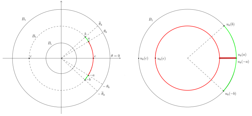
Figure 2: Source and target of the map $u_{k}$ in the example of Section 4.2. The small interior circle in the right figure is a $t$-slice of a catenoid, whereas the horizontal segment is the $t$-section of the flap. The radius of the small circle is $\overline{\rho}(l)$.

To define $u_{k}$ on ${\rm B}_{r_{k}}$ we adopt a construction similar to the one in (4.1). First of all, $u_{k}(0,0):=(-1,0)$. Then, in ${\rm B}_{r_{k}}\cap\{\alpha\in(-\pi,\pi)\setminus(-\overline{\theta}_{k},\overline{\theta}_{k})\}$ we impose $u_{k}$ as in (4.1) with $\overline{\theta}_{k}$ replacing $\alpha_{k}$. In ${\rm B}_{r_{k}}\cap\{\alpha\in(-\overline{\theta}_{k},\overline{\theta}_{k})\}$ we require

$$u_{k}([0,r_{k}],\alpha):=\partial B_{1}\cap\{\pm\theta\in((u_{k})_{2}(r_{k},\alpha),\pi)\},\qquad\pm\alpha\in(0,\pi],$$

where $(u_{k})_{2}$ is the second (angular) coordinate of $u_{k}$.

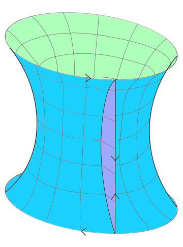
Figure 3: Catenoid union a flap, namely the set $CF$ (Section 4.2).

Hence

$$u_{k}(\partial{\rm B}_{t})\begin{cases}\subsetneq\partial B_{1}\qquad&\text{if }t\in(0,{r_{k}}],\\ =(\partial B_{1})\cup\{(r,0)\in\overline{B}_{1}:r\in[\rho(t),1]\}\cup(\partial B_{\rho(t)})\qquad&\text{if }t\in({r_{k}},l).\end{cases}$$

Remark 4.2.

Also in this case $(u_{k})$ is not a recovery sequence, due to Theorem 3.4, and the results in [8, 9]. For this particular sequence we have

$$\lim_{k\to+\infty}\mathcal{A}(u_{k},\Omega)=\int_{\Omega}|\mathcal{M}(\nabla u)|~{}dx+\mathcal{H}^{2}({\rm catenoid})+2\,\mathcal{H}^{2}({\rm flap}).$$

This surface is not a minimizer of problem on the right-hand side of (3.5). However it is worth noticing that, by minimality property of the catenoid, it can be proved that the set $CF$, treated as an integral current, is $S_{\textrm{min}}$, the minimal vertical current closing the graph $\mathcal{G}_{u}$ of the vortex map in $\Omega$ (see the discussion in the Introduction).

4.3 The case of two discs

In [1], the authors describe a sequence $(u_{k})$ of maps converging to the vortex map $u$, simply defined as follows:

$${u_{k}}(r,\alpha):=\phi_{k}(r)u(r,\alpha),$$ (4.2)

where $\phi_{k}:[0,l]\to[0,1]$ is a smooth function such that $\phi_{k}=0$ in $[0,\frac{1}{k^{2}}]$, $\phi_{k}=1$ in $[\frac{1}{k},l]$, and $0\leq\phi_{k}^{\prime}\leq 2k$. In this case $(u_{k})$ is a recovery sequence for $l$ sufficiently large, due to [1, Lemma 4.2]. We have

$$\lim_{k\to+\infty}\mathcal{A}(u_{k},\Omega)=\int_{\Omega}|\mathcal{M}(\nabla u)|~{}dx+\pi,$$

and $\pi$ has the meaning of the area of the unit disc. This surface, for $l$ sufficiently large, is a minimizer of problem on the right-hand side of (3.5) (where it corresponds to $h\equiv-1$).

5 Proof of Theorem 3.4

In this section we prove Theorem 3.4. To this aim, we need to construct a sequence $({u_{k}})\subset\textrm{Lip}({\Omega},\mathbb{R}^{2})$ converging to $u$ in $L^{1}({\Omega},\mathbb{R}^{2})$ such that

$$\lim_{k\to+\infty}\mathcal{A}({u_{k}},{\Omega})\leq\int_{{\Omega}}|\mathcal{M}(\nabla u)|dx+{\mathcal{F}}_{2l}({h^{\star}},\psi^{\star}),$$

where $({h^{\star}},\psi^{\star})$ is a pair minimizing ${\mathcal{F}}_{2l}$ as in Theorem 3.2. We may assume that $h^{\star}$ is not identically $-1$, otherwise the result follows from [1] (and a recovery sequence is provided as in (4.2)).

We will specify various subsets of ${\Omega}$ and define the sequence $({u_{k}})$ on each of these sets (see Fig. 4). More precisely, we will define $u_{k}$ as a map taking values in $\mathbb{S}^{1}$ in the largest sector (step 1). This construction is similar to the one in [1] (see also Remark 5.1 below). The contribution of the area in this sector will equal, as $k\rightarrow+\infty$, the first term in (3.14). The second term will be instead provided by the contribution of $u_{k}$ in region $C_{k}\setminus B_{r_{k}}$ (step 2), where we will need the aid of the functions $({h^{\star}},\psi^{\star})$ (suitably regularized, in order to render $u_{k}$ Lipschitz continuous). The other regions surrounding $C_{k}\setminus B_{r_{k}}$ are needed to glue $u_{k}$ between the aforementioned regions. This is done in steps 3, 4 and 5, where it is also proven that the corresponding area contribution is negligible. Finally, in steps 6 and 7 we show the crucial estimates to prove (3.14). In Fig. 4 this subdivion of the domain $\Omega$ is drawn.

Remark 5.1.

Our construction differs from the one in [1], even when in place of $({h^{\star}},\psi^{\star})$ we use $(1,\sqrt{1-s^{2}})$ (i.e., the one in Section 4.1) in the following sense. We use the full graph of $\pm\psi^{\star}$ to construct $u_{k}$ and therefore, in the case when $({h^{\star}},\psi^{\star})$ is replaced by $(1,\sqrt{1-s^{2}})$, the image of $u_{k}$ covers the whole cylinder and not only a part of it. Since $h^{\star}$ may be not identically $1$ (and actually is not explicit in general), the presence of a new set $T_{k}$ is now needed, as an intermediate region to glue the trace of $u_{k}$ along the two segments $\{\alpha=\pm\overline{\theta}_{k}\}$. The image set $u_{k}(T_{k})$ covers a small part of the unit circle. See Fig. 4, where $T_{k}$ is represented as the union of the two thin sectors in $\Omega$. To glue all the piecese in order that $u_{k}$ is Lipschitz, it will be useful to have two transition regions, one in a ball $B_{r_{k}/2}$ and one in the annulus $B_{r_{k}}\setminus B_{r_{k}/2}$. It is worth noticing that the curve $u_{k}\mathop{\hbox{\vrule height=7.0pt,width=0.5pt,depth=0.0pt\vrule height=0.5pt,width=6.0pt,depth=0.0pt}}\nolimits\partial{\rm B}_{t}$ has null winding number around the origin, for all $t\in(0,l)$.

Let $k\in\mathbb{N}$ and let $({r_{k}}),(\theta_{k}),(\overline{\theta}_{k})$ be infinitesimal sequences of positive numbers such that $\overline{\theta}_{k}-\theta_{k}=:\delta_{k}>0$. We suppose

$$\lim_{k\to+\infty}(\theta_{k}k)=0.$$ (5.1)

Let ${{\rm B}_{r_{k}}}$ be the open disc centered at the origin with radius ${r_{k}}$, and

$${{C}_{k}}:=\{(r,\alpha)\in[0,l)\times[0,2\pi):\alpha\in[0,\theta_{k}]\cup[2\pi-\theta_{k},2\pi)\},$$ (5.2)

be the half-cone in $\Omega$, with vertex at the origin and aperture equal to $2\theta_{k}$, see Fig. 4. We set

$$C_{k}^{+}:=C_{k}\cap\{\alpha\in[0,\theta_{k}]\},\quad C_{k}^{-}:=C_{k}\cap\{\alpha\in[2\pi-\theta_{k},2\pi]\},$$

and we divide ${{C}_{k}}\cap({\Omega}\setminus{{\rm B}_{r_{k}}})$ into two sets

$$C_{k}\setminus{{\rm B}_{r_{k}}}:=\big{(}C_{k}^{+}\setminus{{\rm B}_{r_{k}}}\big{)}\cup\big{(}C_{k}^{-}\setminus{{\rm B}_{r_{k}}}\big{)}.$$ (5.3)

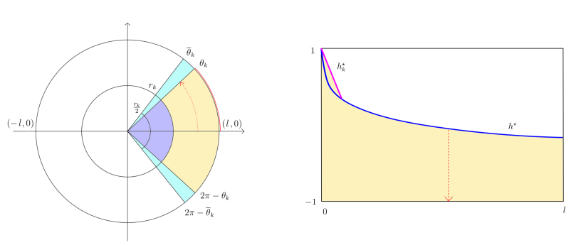
Figure 4: On the left the subdivision of ${\rm B}_{l}$ in sectors. Specifically, the sectors $C_{k}^{+}\setminus{{\rm B}_{r_{k}}}$ and $C_{k}^{-}\setminus{{\rm B}_{r_{k}}}$ are emphasized in light grey. The map $\mathcal{T}_{k}$ defined in (5.18) sends $C_{k}^{+}\setminus{{\rm B}_{r_{k}}}$ in the (reflected) subgraph of $h^{\star}_{k}$ in $R_{l}$, depicted on the right; it maps the segment joining $(r_{k},0)$ to $(1,0)$ onto the graph of $h^{\star}_{k}$, and the radius corresponding to $\alpha=\theta_{k}$ onto the basis of $R_{l}$, following the orientation emphasized by the dashed arrow. The graph of $h^{\star}_{k}$ starts linearly from the point $(0,1)$ in the interval $[0,1/k)$ with negative derivative, then joins (and next coincides) with the graph of $h^{\star}$. The definition of $u_{k}$ in $C_{k}^{+}\setminus{{\rm B}_{r_{k}}}$ makes use of this parametrization of $SG_{h^{\star}_{k}}\cap\overline{R}_{l}$ (see (5.21)). This parametrization needs a reflection, in order to glue $u_{k}$ on the horizontal segment $\{\alpha=0\}$ with the definition of $u_{k}$ in $C_{k}^{-}\setminus{{\rm B}_{r_{k}}}$.

Finally, let

$$T_{k}:=\{(r,\alpha)\in[0,l)\times[0,2\pi):\alpha\in[\theta_{k},\overline{\theta}_{k}]\cup[2\pi-\overline{\theta}_{k},2\pi-\theta_{k}]\}.$$ (5.4)

Step 1. Definition of ${u_{k}}$ on $\overline{{\Omega}\setminus({{C}_{k}}\cup T_{k})}$.

In this step our construction is similar to the one in [1, Lem. 5.3], see also (4.1); in order to define $u_{k}$, in the source we use polar coordinates $(r,\alpha)$ and Cartesian coordinates in the target. Define

$${u_{k}}(r,\alpha):=\begin{cases}u(r,\alpha)=(\cos\alpha,\sin\alpha),&r\in(r_{k}/2,l),\alpha\in[\overline{\theta}_{k},2\pi-\overline{\theta}_{k}],\\ \Big{(}\cos(\frac{2r}{{r_{k}}}(\alpha-\pi)+\pi),\sin(\frac{2r}{{r_{k}}}(\alpha-\pi)+\pi)\Big{)},&r\in[0,r_{k}/2],\alpha\in[\overline{\theta}_{k},2\pi-\overline{\theta}_{k}].\end{cases}$$ (5.5)

Obviously

$${u_{k}}(0,0)=(-1,0)=u_{k}(r,\pi),\qquad r\in[0,l),$$

$${u_{k}}(r,\overline{\theta}_{k})=(\cos\overline{\theta}_{k},\sin\overline{\theta}_{k}),\qquad{u_{k}}(r,2\pi-\overline{\theta}_{k})=(\cos\overline{\theta}_{k},\sin(-\overline{\theta}_{k})),\qquad r\in({r_{k}}/2,l),$$

$${u_{k}}(r,\overline{\theta}_{k})=\Big{(}\cos(\frac{2r}{{r_{k}}}(\overline{\theta}_{k}-\pi)+\pi)~{},~{}\sin(\frac{2r}{{r_{k}}}(\overline{\theta}_{k}-\pi)+\pi)\Big{)},\qquad r\in[0,{r_{k}}/2],$$

$${u_{k}}(r,2\pi-\overline{\theta}_{k})=\Big{(}\cos(\frac{2r}{{r_{k}}}(\pi-\overline{\theta}_{k})+\pi)~{},~{}\sin(\frac{2r}{{r_{k}}}(\pi-\overline{\theta}_{k})+\pi)\Big{)},\qquad r\in[0,{r_{k}}/2].$$ (5.6)

The relevant contribution to the area of the graph of $u_{k}$ is the one in region $C_{k}$, and more specifically in $C_{k}\setminus B_{r_{k}}$; it is in this region that we need to use a minimizing pair of ${\mathcal{F}}_{2l}$.

Step 2. Definition of ${u_{k}}$ on ${{C}_{k}}\setminus{{\rm B}_{r_{k}}}$.

We first need a regularization of $h^{\star}$: assuming without loss of generality $1/k<l$, we define

$$h^{\star}_{k}(w_{1}):=\begin{cases}h^{\star}(w_{1})&{\rm for~{}}w_{1}\in[\frac{1}{k},l],\\ k\left(h^{\star}(\frac{1}{k})-{h^{\star}}(0)\right)w_{1}+{h^{\star}}(0)&{\rm for~{}}w_{1}\in[0,\frac{1}{k}),\end{cases}$$ (5.7)

where we recall that $h^{\star}(0)=1$ (see Theorem 3.2), and we set $h^{\star}_{k}(w_{1}):=h^{\star}_{k}(2l-w_{1})$ for $w_{1}\in[l,2l]$ (see Fig. 4, right). Notice that ${h^{\star}_{k}}(0)=1$, $h^{\star}_{k}\in{\rm Lip}([0,2l])$ and the convexity of $h^{\star}$ implies that also $h^{\star}_{k}$ is convex, $h^{\star}_{k}\geq h^{\star}$, and therefore by Lemma 3.3 (i) we see that $(h^{\star}_{k},\psi^{\star}_{k})\in X_{2l}^{{\rm conv}}$, where $\psi^{\star}_{k}$ is the approximation of $\psi^{\star}$ considered in Lemma 3.3 (with $k=m$), see formula (3.12). Again by Lemma 3.3, ${\mathcal{F}}_{2l}(h^{\star}_{k},\psi^{\star}_{k})={\mathcal{F}}_{2l}(h^{\star},\psi^{\star}_{k})+\int_{0}^{2l}\left(h^{\star}_{k}(w_{1})-h^{\star}(w_{1})\right)~{}dw_{1}\rightarrow{\mathcal{F}}_{2l}(h^{\star},\psi^{\star})$ as $k\rightarrow+\infty$.

We start with the construction of $u_{k}$ on $C_{k}^{+}\setminus{{\rm B}_{r_{k}}}$. Set

$$\tau_{k}:[{r_{k}},l]\to[0,l], \tau_{k}(r):=\frac{l}{l-{r_{k}}}(r-{r_{k}}),$$ (5.8)

$$s_{k}:[{r_{k}},l]\times[0,\theta_{k}]\to[-1,1], s_{k}(r,\alpha):=\frac{1+{h^{\star}_{k}}(\tau_{k}(r))}{\theta_{k}}\alpha-{h^{\star}_{k}}(\tau_{k}(r)).$$ (5.9)

Note that $s_{k}(r,\cdot):[0,\theta_{k}]\to[-{h^{\star}_{k}}(\tau_{k}(r)),1]$ is a bijective increasing function, for any $r\in[r_{k},l]$, and

$$s_{k}(r,0)=-{h^{\star}_{k}}(\tau_{k}(r))\quad{\rm for~{}any}~{}r\in[r_{k},l],\text{ in particular }s_{k}({r_{k}},0)=-1,$$ (5.10)

$$s_{k}(r,\theta_{k})=1,\qquad r\in[{r_{k}},l],$$ (5.11)

$$s_{k}(r_{k},\alpha)=\frac{2\alpha}{\theta_{k}}-1,\qquad\alpha\in[0,\theta_{k}].$$ (5.12)

We have, for all $r\in[{r_{k}},l]$ and $\alpha\in[0,\theta_{k}]$,

$$\tau_{k}^{\prime}(r)=\frac{l}{l-{r_{k}}},$$ (5.13)

$$\partial_{\alpha}s_{k}(r,\alpha)=\frac{1+{h^{\star}_{k}}(\tau_{k}(r))}{\theta_{k}},$$ (5.14)

and, for almost every $r\in[{r_{k}},l]$ and all $\alpha\in[0,\theta_{k}]$,

$$\partial_{r}s_{k}(r,\alpha)=\left(\frac{\alpha}{\theta_{k}}-1\right)\tau_{k}^{\prime}(r){h^{\star}_{k}}^{\prime}(\tau_{k}(r))=\frac{l}{l-{r_{k}}}\left(\frac{\alpha}{\theta_{k}}-1\right){h^{\star}_{k}}^{\prime}(\tau_{k}(r)).$$ (5.15)

Moreover we define

$$H_{k}:[0,l]\to[{r_{k}},l],\qquad H_{k}({w_{1}}):=\frac{l-{r_{k}}}{l}{w_{1}}+{r_{k}}~{}$$ (5.16)

to be the inverse of $\tau_{k}$ and, recalling that $\overline{R}_{l}=[0,l]\times[-1,1]$,

$$\Theta_{k}:SG_{{h^{\star}_{k}}}\cap\overline{R}_{l}\to[0,\theta_{k}],\qquad\Theta_{k}({w_{1}},{w_{2}}):=\frac{\theta_{k}}{1+{h^{\star}_{k}}({w_{1}})}({h^{\star}_{k}}({w_{1}})-{w_{2}}).$$ (5.17)

Notice that $\Theta_{k}({w_{1}},\cdot):[-1,{h^{\star}_{k}}({w_{1}})]\to[0,\theta_{k}]$ is a linearly decreasing bijective function

The map

$$\mathcal{T}_{k}:C_{k}^{+}\setminus{{\rm B}_{r_{k}}}\to SG_{{h^{\star}_{k}}}\cap\overline{R}_{l},\qquad\mathcal{T}_{k}(r,\alpha):=(\tau_{k}(r),-s_{k}(r,\alpha)),$$ (5.18)

is invertible, and its inverse is the map

$$\mathcal{T}_{k}^{-1}:SG_{{h^{\star}_{k}}}\cap\overline{R}_{l}\to C_{k}^{+}\setminus{{\rm B}_{r_{k}}},\qquad\mathcal{T}_{k}^{-1}({w_{1}},{w_{2}}):=(H_{k}({w_{1}}),\Theta_{k}({w_{1}},{w_{2}})).$$ (5.19)

The modulus of the determinant of the Jacobian of $\mathcal{T}_{k}^{-1}$ is given by

$$|J_{\mathcal{T}_{k}^{-1}}|=\left(\frac{l-{r_{k}}}{l}\right)\frac{\theta_{k}}{1+{h^{\star}_{k}}({w_{1}})}.$$ (5.20)

We set

$${u_{k}}(r,\alpha):=\Big{(}s_{k}(r,\alpha),\psi^{\star}_{k}\big{(}\mathcal{T}_{k}(r,\alpha)\big{)}\Big{)}=\Big{(}u_{k1}(r,\alpha),u_{k2}(r,\alpha)\Big{)},\qquad r\in[r_{k},l],\alpha\in[0,\theta_{k}].$$ (5.21)

Observe that, using the definition of $\psi_{k}^{\star}$,

$${u_{k}}\in{\rm Lip}(C_{k}^{+}\setminus{{\rm B}_{r_{k}}},\mathbb{R}^{2}),$$ (5.22)

$${u_{k}}(r,\theta_{k})=(s_{k}(r,\theta_{k}),\psi_{k}^{\star}(\mathcal{T}_{k}(r,\theta_{k})))=(1,0),$$

$${u_{k}}(r,0)=(-{h^{\star}_{k}}(\tau_{k}(r)),\psi^{\star}_{k}(\tau_{k}(r),{h^{\star}_{k}}(\tau_{k}(r))))=(-{h^{\star}_{k}}(\tau_{k}(r)),0),$$

$${u_{k}}({r_{k}},\alpha)=(s_{k}({r_{k}},\alpha),\psi^{\star}_{k}(0,-s_{k}({r_{k}},\alpha)))=(s_{k}({r_{k}},\alpha),\varphi_{k}(0,-s_{k}({r_{k}},\alpha))),$$

for $r\in[r_{k},l]$ and $\alpha\in[0,\theta_{k}]$, as it follows from (5.8), (5.10), (5.11), and (3.8), where $\varphi_{k}$ is defined in (3.11) (with $k=m$).

Eventually we define $u_{k}$ on $C_{k}^{-}\setminus{{\rm B}_{r_{k}}}$ as

$${u_{k}}(r,\alpha):=(u_{k1}(r,2\pi-\alpha),-u_{k2}(r,2\pi-\alpha)),\qquad r\in[r_{k},l],\alpha\in[2\pi-\theta_{k},2\pi).$$ (5.23)

It turns out

$${u_{k}}\in{\rm Lip}(C_{k}^{-}\setminus{{\rm B}_{r_{k}}},\mathbb{R}^{2}),$$

$${u_{k}}(r,2\pi-\theta_{k})=(1,0),$$

$${u_{k}}(r,2\pi)=(-{h^{\star}_{k}}(\tau_{k}(r)),-\psi^{\star}_{k}(\tau_{k}(r),{h^{\star}_{k}}(\tau_{k}(r))))=(-{h^{\star}_{k}}(\tau_{k}(r)),0),$$

$${u_{k}}({r_{k}},\alpha)=(s_{k}({r_{k}},2\pi-\alpha),-\psi^{\star}_{k}(0,-s_{k}({r_{k}},2\pi-\alpha))),$$

for $r\in[r_{k},l]$, $\alpha\in[2\pi-\theta_{k},2\pi)$.

The area of the graph of $u_{k}$ on $C_{k}\setminus B_{r_{k}}$ will be computed in step 7.

Step 3. Definition of ${u_{k}}$ on ${{C}_{k}}\cap(\overline{B}_{r_{k}}\setminus{\rm B}_{r_{k}/2})$ and its area contribution.

Let $G_{\psi^{\star}_{k}(0,\cdot)}\subset\mathbb{R}^{2}$ (resp. $G_{\psi^{\star}(0,\cdot)}\subset\mathbb{R}^{2}$) denote the graph of $\psi^{\star}_{k}(0,\cdot)$ (resp. of $\psi^{\star}(0,\cdot)$) on $[-1,1]$. We introduce the retraction map $\Upsilon:(\mathbb{R}\times[0,+\infty))\setminus O\subset\mathbb{R}^{2}_{{\rm target}}\rightarrow G_{\psi^{\star}(0,\cdot)}\subset\mathbb{R}^{2}_{{\rm target}}$, $O=(0,0)$, defined by

$$\Upsilon(p)=q:=G_{\psi^{\star}(0,\cdot)}\cap\ell_{Op}\qquad\forall p\in(\mathbb{R}\times[0,+\infty))\setminus O,$$

where $\ell_{Op}$ is the line passing through $O$ and $p$. Then $\Upsilon$ is well-defined and it is Lipschitz continuous in a neighbourhood of $G_{\psi^{\star}(0,\cdot)}$ in $\mathbb{R}\times[0,+\infty)$. We also define

$$\Upsilon_{k}:G_{\psi^{\star}_{k}(0,\cdot)}\rightarrow G_{\psi^{\star}(0,\cdot)}$$

as the restriction of $\Upsilon$ to $G_{\psi^{\star}_{k}(0,\cdot)}$; see Fig. 5. As a consequence, since for $k\in\mathbb{N}$ large enough $G_{\psi_{k}^{\star}(0,\cdot)}$ is contained in a neighbourhood of $G_{\psi^{\star}(0,\cdot)}$, we have that $\Upsilon_{k}$ is Lipschitz continuous with Lipschitz constant independent of $k$. Notice also that $\Upsilon_{k}((-1,0))=(-1,0)$ and $\Upsilon_{k}((1,0))=(1,0)$.

We define $u_{k}$ on $C_{k}^{+}\cap(\overline{\rm B}_{r_{k}}\setminus{\rm B}_{r_{k}/2})$ setting, for $r\in[\frac{r_{k}}{2},r_{k}]$ and $\alpha\in[0,\theta_{k}]$,

$$u_{k}(r,\alpha):=\Big{(}2-\frac{2r}{r_{k}}\Big{)}\Upsilon_{k}\big{(}s_{k}(r_{k},\alpha),\psi_{k}^{\star}(0,-s_{k}(r_{k},\alpha))\big{)}+\Big{(}\frac{2r}{r_{k}}-1\Big{)}\big{(}s_{k}(r_{k},\alpha),\psi_{k}^{\star}(0,-s_{k}(r_{k},\alpha))\big{)}.$$

We have

$$u_{k}(r_{k},\alpha)=(s_{k}(r_{k},\alpha),\psi_{k}^{\star}(0,-s_{k}(r_{k},\alpha))),$$

so that $u_{k}$ glues, on $C_{k}^{+}\cap\partial{\rm B}_{r_{k}}$, with the values obtained in step 2 (last formula in (5.22)), and

$$u_{k}(r,\theta_{k})=(1,0),\qquad u_{k}(r,0)=(-1,0).$$

This formula shows that $u_{k}$ also glues, on $C_{k}^{+}\cap\{(r,\alpha):r\in[r_{k}/2,r_{k}],\alpha\in\{0,\theta_{k}\}\}$, with the values obtained in step 2 (second and third formula in (5.22)). Moreover

$$u_{k}(r_{k}/2,\alpha)=\Upsilon_{k}\big{(}s_{k}(r_{k},\alpha),\psi_{k}^{\star}(0,-s_{k}(r_{k},\alpha))\big{)},\qquad\alpha\in[0,\theta_{k}].$$ (5.24)

In addition, using (5.12), the derivatives of $u_{k}$ satisfy, for $r\in(\frac{r_{k}}{2},r_{k})$ and $\alpha\in(0,\theta_{k})$,

$$\partial_{r}u_{k}(r,\alpha)=-\frac{2}{r_{k}}\Upsilon_{k}\big{(}s_{k}(r_{k},\alpha),\psi_{k}^{\star}(0,-s_{k}(r_{k},\alpha))\big{)}+\frac{2}{r_{k}}\big{(}s_{k}(r_{k},\alpha),\psi_{k}^{\star}(0,-s_{k}(r_{k},\alpha))\big{)},$$

$$\partial_{\alpha}u_{k}(r,\alpha)=\Big{(}2-\frac{2r}{r_{k}}\Big{)}\nabla\Upsilon_{k}\big{(}s_{k}(r_{k},\alpha),\psi_{k}^{\star}(0,-s_{k}(r_{k},\alpha))\big{)}\cdot\Big{(}\frac{2}{\theta_{k}},-\frac{2}{\theta_{k}}\partial_{w_{2}}\psi_{k}^{\star}(0,-s_{k}(r_{k},\alpha))\Big{)}$$

$$\qquad\qquad\qquad+\Big{(}\frac{2r}{r_{k}}-1\Big{)}\Big{(}\frac{2}{\theta_{k}},-\frac{2}{\theta_{k}}\partial_{w_{2}}\psi_{k}^{\star}(0,-s_{k}(r_{k},\alpha))\Big{)},$$

so that

$$|\partial_{r}u_{k}(r,\alpha)|\leq\frac{4}{r_{k}},$$

$$|\partial_{\alpha}u_{k}(r,\alpha)|\leq\frac{2(\widehat{C}+1)}{\theta_{k}}(|\partial_{w_{2}}\psi_{k}^{\star}(0,-s_{k}(r_{k},\alpha))|+1),$$

where $\widehat{C}$ is a positive constant independent of $k$, which bounds the gradient of $\Upsilon_{k}$. Since $\psi_{k}^{\star}$ is Lipschitz, we deduce that $u_{k}$ is Lipschitz continuous on $C_{k}^{+}\cap({{\rm B}_{r_{k}}}\setminus{\rm B}_{r_{k}/2})$.

Furthermore the image of $(\frac{r_{k}}{2},r_{k})\times(0,\theta_{k})$ through the map $(r,\alpha)\mapsto u_{k}(r,\alpha)$ is the region enclosed by $G_{\psi^{\star}_{k}}$ and $G_{\psi^{\star}}$ (with multiplicity $1$). The area of this region is infinitesimal as $k\rightarrow+\infty$, so that, by the area formula,

$$\int_{r_{k}/2}^{r_{k}}\int_{0}^{\theta_{k}}r|Ju_{k}(r,\alpha)|d\alpha dr=o(1)\qquad{\rm as~{}}k\rightarrow+\infty.$$

Hence, using the fact that the gradient in polar coordinates is $(\partial_{r},\frac{1}{r}\partial_{\alpha})$, we eventually estimate

$$\int_{r_{k}/2}^{r_{k}}\int_{0}^{\theta_{k}}r|\mathcal{M}(\nabla u_{k})|d\alpha dr \leq\int_{r_{k}/2}^{r_{k}}\int_{0}^{\theta_{k}}\Big{(}r+\frac{4r}{r_{k}}+\frac{C}{\theta_{k}}|\partial_{w_{2}}\psi_{k}^{\star}(0,1-\frac{2\alpha}{\theta_{k}})|+\frac{C}{\theta_{k}}\Big{)}~{}d\alpha dr+o(1),$$

$$=o(1)+C\frac{r_{k}}{2\theta_{k}}\int_{0}^{\theta_{k}}|\partial_{w_{2}}\psi_{k}^{\star}(0,1-\frac{2\alpha}{\theta_{k}})|d\alpha=o(1)$$ (5.25)

as $k\rightarrow+\infty$. In the last equality we use that $|\partial_{w_{2}}\psi^{\star}_{k}(0,\cdot)|\leq|\partial_{w_{2}}\psi^{\star}(0,\cdot)|$, which is integrable via the change of variables $w_{2}=1-\frac{2\alpha}{\theta_{k}}$ (it also makes $\theta_{k}$ disappear at the denominator in front of the integral in (5)).

This proves that the contribution of area of the graph of $u_{k}$ over $C_{k}^{+}\cap({{\rm B}_{r_{k}}}\setminus{\rm B}_{r_{k}/2})$ is infinitesimal as $k\rightarrow+\infty$.

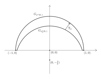
Figure 5: the graphs of the functions $\psi^{\star}_{k}(0,\cdot)$ and $\psi^{\star}(0,\cdot)$; these contain arcs of circle centered at $(0,0)$ and $(0,-\frac{2}{k})$ respectively. The map $\Upsilon_{k}$ is emphasized, and turns out to be the restriction of $x\mapsto\frac{x}{|x|}$ on $\psi^{\star}_{k}(0,\cdot)$.

Eventually, for $r\in[r_{k}/2,r_{k}]$, $\alpha\in[2\pi-\theta_{k},2\pi)$, we set

$$u_{k}(r,\alpha):=(u_{k1}(r,2\pi-\alpha),-u_{k2}(r,2\pi-\alpha)).$$ (5.26)

Observe that, thanks to (5.23), $u_{k}$ is continuous on $\partial{\rm B}_{r_{k}}$, and similar estimates as in (5) hold on $({\rm B}_{r_{k}}\setminus{\rm B}_{r_{k}/2})\cap C_{k}^{-}$.

Step 4. Definition of ${u_{k}}$ on ${{C}_{k}}\cap{\rm B}_{r_{k}/2}$ and its area contribution.

We start with the construction of $u_{k}$ on $C_{k}^{+}\cap{\rm B}_{r_{k}/2}$. For $r\in[0,r_{k}/2]$ and $\alpha\in[0,\theta_{k}]$ we set

$$u_{k}(r,\alpha):=\Upsilon_{k}\Big{(}\frac{4r\alpha}{r_{k}\theta_{k}}-1,\psi_{k}^{\star}\big{(}0,1-\frac{4r\alpha}{r_{k}\theta_{k}}\big{)}\Big{)}.$$ (5.27)

First we observe that

$$u_{k}\Big{(}\frac{r_{k}}{2},\alpha\Big{)}=\Upsilon_{k}\Big{(}\frac{2\alpha}{\theta_{k}}-1,\psi_{k}^{\star}\big{(}0,1-\frac{2\alpha}{\theta_{k}}\big{)}\Big{)},\qquad\alpha\in(0,\theta_{k}),$$

so that $u_{k}$ is continuous on $C_{k}^{+}\cap\partial{\rm B}_{r_{k}/2}$ (see (5.24) and (5.12)), and

$$u_{k}(r,\theta_{k})=\Upsilon_{k}\Big{(}\frac{4r}{r_{k}}-1,\psi_{k}^{\star}(0,1-\frac{4r}{r_{k}})\Big{)},$$ (5.28)

$$u_{k}(r,0)=(-1,\psi_{k}^{\star}(0,1))=(-1,0).$$ (5.29)

Direct computations lead to the following estimates:

$$|\partial_{r}u_{k}(r,\alpha)|\leq\widehat{C}\frac{4\alpha}{r_{k}\theta_{k}}\Big{(}1+|\partial_{w_{2}}\psi^{\star}_{k}(0,1-\frac{4\alpha r}{r_{k}\theta_{k}})|\Big{)},$$ (5.30)

$$|\partial_{\alpha}u_{k}(r,\alpha)|\leq\widehat{C}\frac{4r}{r_{k}\theta_{k}}\Big{(}1+|\partial_{w_{2}}\psi^{\star}_{k}(0,1-\frac{4\alpha r}{r_{k}\theta_{k}})|\Big{)},$$ (5.31)

where $\widehat{C}$ is the constant bounding the gradient of $\Upsilon_{k}$ as in step 3. Finally, since by (5.27) $u_{k}$ takes values in $\mathbb{S}^{1}\subset\mathbb{R}^{2}$, we have $Ju_{k}(r,\alpha)=0$ for all $r\in(0,r_{k}/2)$, $\alpha\in[0,\theta_{k}]$. Hence, the area of the graph of $u_{k}$ on $C_{k}^{+}\cap{\rm B}_{r_{k}/2}$ is

$$\int_{0}^{r_{k}/2}\int_{0}^{\theta_{k}}r|\mathcal{M}(\nabla u_{k})(r,\alpha)|~{}d\alpha dr\leq\int_{0}^{r_{k}/2}\int_{0}^{\theta_{k}}(r+C)+\frac{C}{\theta_{k}}+\frac{Cr}{r_{k}}(1+\frac{1}{\theta_{k}})|\partial_{w_{2}}\psi^{\star}_{k}(0,1-\frac{4\alpha r}{r_{k}\theta_{k}})|d\alpha dr,$$

where $C$ is a positive constant independent of $k$. Exploiting that $|\partial_{w_{2}}\psi^{\star}_{k}(0,\cdot)|\leq|\partial_{w_{2}}\psi^{\star}(0,\cdot)|$, we can estimate the right-hand side of the previous formula as follows:

$$C\int_{0}^{r_{k}/2}\int_{0}^{\theta_{k}}\frac{r}{r_{k}}\Big{(}1+\frac{1}{\theta_{k}}\Big{)}|\partial_{w_{2}}\psi^{\star}(0,1-\frac{4\alpha r}{r_{k}\theta_{k}})|d\alpha dr+o(1)$$ (5.32)

$$\leq C\int_{0}^{r_{k}/2}\int_{-1}^{1}\theta_{k}\Big{(}1+\frac{1}{\theta_{k}}\Big{)}|\partial_{w_{2}}\psi^{\star}(0,w_{2})|dw_{2}dr+o(1)$$

$$\leq C\int_{0}^{r_{k}/2}(\theta_{k}+1)dr+o(1)=o(1),$$

where $o(1)\rightarrow 0$ as $k\rightarrow+\infty$, and $C$ is a positive constant independent of $k$ which might change from line to line.

In $C_{k}^{-}\cap{\rm B}_{r_{k}/2}$ we set, for $r\in[0,r_{k}/2)$, $\alpha\in[2\pi-\theta_{k},2\pi)$,

$$u_{k}(r,\alpha):=(u_{k1}(r,2\pi-\alpha),-u_{k2}(r,2\pi-\alpha)).$$

Similar estimates as in (5.32) for the area of the graph of $u_{k}$ hold on $C_{k}^{-}\cap{\rm B}_{r_{k}/2}$.

Step 5. Definition of ${u_{k}}$ on $T_{k}$ and its area contribution.

We first construct $u_{k}$ on $T_{k}\cap\{(r,\alpha):r\in[0,r_{k}/2],\alpha\in[\theta_{k},\overline{\theta}_{k}]\}$. We define $\beta_{k}:[0,r_{k}/2]\times[\theta_{k},\overline{\theta}_{k}]\rightarrow[0,\pi]$ as

$$\beta_{k}(r,\alpha):=\frac{\overline{\theta}_{k}-\alpha}{\overline{\theta}_{k}-\theta_{k}}\alpha_{k}(r)+(1-\frac{\overline{\theta}_{k}-\alpha}{\overline{\theta}_{k}-\theta_{k}})\big{(}\frac{2r}{r_{k}}(\overline{\theta}_{k}-\pi)+\pi\big{)},$$

where

$$\alpha_{k}(r):=\arccos\big{(}\Upsilon_{k1}(\frac{4r}{r_{k}}-1,\psi^{\star}_{k}(0,1-\frac{4r}{r_{k}}))\big{)},\qquad r\in[0,r_{k}/2].$$

Notice that $\alpha_{k}$ is decreasing and takes values in $[0,\pi]$. Therefore we set

$$u_{k}(r,\alpha):=\big{(}\cos(\beta_{k}(r,\alpha)),\sin(\beta_{k}(r,\alpha))\big{)},\qquad(r,\alpha)\in[0,r_{k}/2]\times[\theta_{k},\overline{\theta}_{k}].$$ (5.33)

One checks that $\beta_{k}(r,\theta_{k})=\alpha_{k}(r)$, $\beta_{k}(r,\overline{\theta}_{k})=\frac{2r}{r_{k}}(\overline{\theta}_{k}-\pi)+\pi$ (see also (5.5)), and

$$\alpha_{k}(r_{k}/2)=0,$$

$$u_{k}(r_{k}/2,\alpha)=\big{(}\cos((1-\frac{\overline{\theta}_{k}-\alpha}{\overline{\theta}_{k}-\theta_{k}})\overline{\theta}_{k}),\sin((1-\frac{\overline{\theta}_{k}-\alpha}{\overline{\theta}_{k}-\theta_{k}})\overline{\theta}_{k})\big{)},$$

$$u_{k}(r,\theta_{k})=\big{(}\cos(\alpha_{k}(r)),\sin(\alpha_{k}(r))\big{)}=\Upsilon_{k}(\frac{4r}{r_{k}}-1,\psi^{\star}_{k}(0,1-\frac{4r}{r_{k}})),$$

$$u_{k}(r,\overline{\theta}_{k})=\big{(}\cos(\frac{2r}{r_{k}}(\overline{\theta}_{k}-\pi)+\pi),\sin(\frac{2r}{r_{k}}(\overline{\theta}_{k}-\pi)+\pi)\big{)},$$

so that $u_{k}$ is continuous on $\{\alpha\in\{\theta_{k},\overline{\theta}_{k}\},\;r\in[0,r_{k}/2]\}\cap\Omega$, see (5.6) and (5.28).

Notice also that $u_{k}$ is continuous at $(0,0)\in\mathbb{R}^{2}$ and $u_{k}(0,0)=(-1,0)$. Finally, since $u_{k}$ in (5.33) takes values in $\mathbb{S}^{1}$, the determinant of its Jacobian vanishes, so that in order to estimate the area contribution of the graph of $u_{k}$ in $T_{k}\cap\{(r,\alpha):r\in[0,r_{k}/2],\;\alpha\in[\theta_{k},\overline{\theta}_{k}]\}$ it is sufficient to estimate the gradient of $u_{k}$. We have

$$|\partial_{r}u_{k}(r,\alpha)|=|\partial_{r}\beta_{k}(r,\alpha)|\leq|\partial_{r}\alpha_{k}(r)|+\frac{2\pi}{r_{k}},$$

$$|\partial_{\alpha}u_{k}(r,\alpha)|=|\partial_{\alpha}\beta_{k}(r,\alpha)|\leq\frac{|\alpha_{k}(r)|}{\overline{\theta}_{k}-\theta_{k}}+\frac{\pi}{\overline{\theta}_{k}-\theta_{k}}\leq\frac{2\pi}{\overline{\theta}_{k}-\theta_{k}}.$$

Therefore

$$\int_{0}^{r_{k}/2}\int_{\theta_{k}}^{\overline{\theta}_{k}}r|\mathcal{M}(\nabla u_{k})(r,\alpha)|d\alpha dr\leq\int_{0}^{r_{k}/2}\int_{\theta_{k}}^{\overline{\theta}_{k}}\Big{[}\frac{r_{k}}{2}(1+|\partial_{r}\beta_{k}(r,\alpha)|)+|\partial_{\alpha}\beta_{k}(r,\alpha)|\Big{]}~{}d\alpha dr$$

$$\leq o(1)+\int_{0}^{r_{k}/2}\int_{\theta_{k}}^{\overline{\theta}_{k}}\left(\frac{r_{k}}{2}|\partial_{r}\alpha_{k}(r)|+\pi+\frac{2\pi}{\overline{\theta}_{k}-\theta_{k}}\right)d\alpha dr=o(1),$$ (5.34)

with $o(1)\rightarrow 0$ as $k\rightarrow+\infty$. Notice that the integral of $|\partial_{r}\alpha_{k}(r)|$ with respect to $r$ can be computed via the fundamental integration theorem, since $\alpha_{k}$ is monotone.

In $T_{k}\cap\{(r,\alpha):r\in[0,r_{k}/2],\alpha\in[2\pi-\overline{\theta}_{k},2\pi-\theta_{k}]\}$ we set

$$u_{k}(r,\alpha):=(u_{k1}(r,2\pi-\alpha),-u_{k2}(r,2\pi-\alpha)).$$

We now define $u_{k}$ on $T_{k}\cap\{(r,\alpha):r\in(r_{k}/2,l),\alpha\in[\theta_{k},\overline{\theta}_{k}]\}$. We set

$$u_{k}(r,\alpha):=\big{(}\cos((1-\frac{\overline{\theta}_{k}-\alpha}{\overline{\theta}_{k}-\theta_{k}})\overline{\theta}_{k}),\sin((1-\frac{\overline{\theta}_{k}-\alpha}{\overline{\theta}_{k}-\theta_{k}})\overline{\theta}_{k})\big{)}.$$

Then ${u_{k}}\in\textrm{Lip}(T_{k},\mathbb{S}^{1})$, and

$${u_{k}}(r,\theta_{k})=(1,0),\qquad{u_{k}}(r,\overline{\theta}_{k})=(\cos\overline{\theta}_{k},\sin\overline{\theta}_{k})\quad\text{ for }r\in({r_{k}}/2,l),$$

$$\partial_{r}u_{k}(r,\alpha)=0,$$

$$\partial_{\alpha}u_{k}(r,\alpha)=\frac{\overline{\theta}_{k}}{\overline{\theta}_{k}-\theta_{k}}\Big{(}-\sin((1-\frac{\overline{\theta}_{k}-\alpha}{\overline{\theta}_{k}-\theta_{k}})\overline{\theta}_{k}),\cos((1-\frac{\overline{\theta}_{k}-\alpha}{\overline{\theta}_{k}-\theta_{k}})\overline{\theta}_{k})\Big{)}.$$

Hence

$$\int_{r_{k}/2}^{l}\int_{\theta_{k}}^{\overline{\theta}_{k}}r|\mathcal{M}(\nabla u_{k})(r,\alpha)|d\alpha dr\leq\int_{r_{k}/2}^{l}\int_{\theta_{k}}^{\overline{\theta}_{k}}\Big{(}r+\frac{\overline{\theta}_{k}}{\overline{\theta}_{k}-\theta_{k}}\Big{)}~{}d\alpha dr=o(1)$$ (5.35)

as $k\rightarrow+\infty$.

Finally in $T_{k}\cap\{(r,\alpha):r\in(r_{k}/2,l),\alpha\in[2\pi-\overline{\theta}_{k},2\pi-\theta_{k}]\}$ we set

$$u_{k}(r,\alpha):=(u_{k1}(r,2\pi-\alpha),-u_{k2}(r,2\pi-\alpha)).$$

Similar estimates as in (5), (5.35) for the area of the graph of $u_{k}$ hold on $T_{k}\cap\{(r,\alpha):r\in(0,r_{k}/2),\alpha\in[2\pi-\overline{\theta}_{k},2\pi-\theta_{k}]\}$, $T_{k}\cap\{(r,\alpha):r\in(r_{k}/2,l),\alpha\in[2\pi-\overline{\theta}_{k},2\pi-\theta_{k}]\}$, respectively.

Step 6. We claim that

$$\int_{{\Omega}\setminus(C_{k}\cup T_{k})}|\mathcal{M}(\nabla{u_{k}})|dx\longrightarrow\int_{\Omega}|\mathcal{M}(\nabla u)|~{}dx\qquad\text{ as }k\to+\infty,$$ (5.36)

where we recall that $C_{k}\cup T_{k}=\{(r,\alpha)\in{\Omega}:r\in[0,l),\alpha\in[0,\overline{\theta}_{k}]\cup[2\pi-\overline{\theta}_{k},2\pi)\}.$

Indeed, on ${\Omega}\setminus(C_{k}\cup T_{k})$ the maps ${u_{k}}$ and $u$ take values in the circle $\mathbb{S}^{1}$, hence

$$\det(\nabla{u_{k}})=0,\qquad\det(\nabla u)=0,\qquad\text{ in }{\Omega}\setminus(C_{k}\cup T_{k}).$$

Thus

$$\int_{{\Omega}\setminus(C_{k}\cup T_{k})}|\mathcal{M}(\nabla{u_{k}})-\mathcal{M}(\nabla u)|~{}dx\leq\sum_{i=1,2}\int_{{\Omega}\setminus(C_{k}\cup T_{k})}|\nabla({u_{k}}_{i}-u_{i})|~{}dx.$$

From (5.5) we have

$$|\partial_{r}({u_{k}}-u)|=0\qquad\textrm{ in }\quad{\Omega}\setminus({{\rm B}_{r_{k}}}\cup{{C}_{k}}\cup T_{k}),$$ (5.37)

$$|\partial_{r}({u_{k}}-u)|\leq\frac{\pi}{{r_{k}}}\ \quad\textrm{ in }\quad{{\rm B}_{r_{k}}}\setminus({{C}_{k}}\cup T_{k}),$$

$$|\partial_{\alpha}({u_{k}}-u)|=0\qquad\text{ in }\quad{\Omega}\setminus({{\rm B}_{r_{k}}}\cup{{C}_{k}}\cup T_{k}),$$

$$|\partial_{\alpha}({u_{k}}-u)|\leq 2\qquad\textrm{ in }\quad{{\rm B}_{r_{k}}}\setminus({{C}_{k}}\cup T_{k}).$$

Our previous remarks and the fact that ${r_{k}},\theta_{k},(\overline{\theta}_{k}-\theta_{k})\to 0^{+}$ as $k\to+\infty$, imply (5.36).

Step 7. We know from (5), (5.32), (5), and (5.35), that the integral of $|\mathcal{M}(\nabla u_{k})|$ is infinitesimal as $k\rightarrow+\infty$, on the region $({\rm B}_{r_{k}}\cap C_{k})\cup T_{k}$. Therefore it remains to compute the area of the graphs of $u_{k}$ in the region $C_{k}\setminus{\rm B}_{r_{k}}$. We claim that this contribution gives

$$\lim_{k\to+\infty}\int_{{{C}_{k}}\setminus{{\rm B}_{r_{k}}}}|\mathcal{M}(\nabla{u_{k}})|~{}dx\leq 2{\mathcal{F}}_{l}({h^{\star}},\psi^{\star})=\mathcal{A}(\psi^{\star},SG_{{h^{\star}}}).$$ (5.38)

To prove this, we start to compute the area of the graph of ${u_{k}}$ restricted to $C_{k}^{+}\setminus{{\rm B}_{r_{k}}}$. From (5.21), (5.13), (5.15) and (5.14), we have

$$\partial_{r}{u_{k}}_{1}=\Big{(}\frac{\alpha}{\theta_{k}}-1\Big{)}\tau_{k}^{\prime}{h^{\star}_{k}}^{\prime}=\frac{l}{l-{r_{k}}}\Big{(}\frac{\alpha}{\theta_{k}}-1\Big{)}{h^{\star}_{k}}^{\prime},$$ (5.39)

$$\partial_{\alpha}{u_{k}}_{1}=\frac{1+{h^{\star}_{k}}}{\theta_{k}},$$

$$\partial_{r}{u_{k}}_{2}=\tau_{k}^{\prime}\Big{[}\Big{(}1-\frac{\alpha}{\theta_{k}}\Big{)}{h^{\star}_{k}}^{\prime}\partial_{w_{2}}\psi^{\star}_{k}+\partial_{w_{1}}\psi^{\star}_{k}\Big{]}=\frac{l}{l-{r_{k}}}\Big{[}\Big{(}1-\frac{\alpha}{\theta_{k}}\Big{)}{h^{\star}_{k}}^{\prime}\partial_{w_{2}}\psi^{\star}_{k}+\partial_{w_{1}}\psi^{\star}_{k}\Big{]},$$

$$\partial_{\alpha}{u_{k}}_{2}=-\Big{[}\frac{1+{h^{\star}_{k}}}{\theta_{k}}\Big{]}\partial_{w_{2}}\psi^{\star}_{k},$$

$$\partial_{r}{u_{k}}_{1}\partial_{\alpha}{u_{k}}_{2}-\partial_{\alpha}{u_{k}}_{1}\partial_{r}{u_{k}}_{2}=-\left(\frac{1+{h^{\star}_{k}}}{\theta_{k}}\right)\frac{l}{l-{r_{k}}}\partial_{w_{1}}\psi^{\star}_{k},$$

where ${h^{\star}_{k}}^{\prime}$ denotes the derivative of ${h^{\star}_{k}}$ with respect to ${w_{1}}$, ${h^{\star}_{k}},{h^{\star}_{k}}^{\prime}$ are evaluated at $\tau_{k}(r)$, and the two partial derivatives $\partial_{w_{2}}\psi^{\star}_{k}$, $\partial_{w_{1}}\psi^{\star}_{k}$ of $\psi^{\star}_{k}$ with respect to ${w_{2}},{w_{1}}$ are evaluated at $(\tau_{k}(r),-s_{k}(r,\alpha))$. Note carefully that, in the computation of the Jacobian, the terms containing $\partial_{w_{2}}\psi^{\star}_{k}$ cancel each other.

Since ${h^{\star}_{k}}$ is convex, its derivative is nonincreasing, and therefore $\int_{{r_{k}}}^{l}|{h^{\star}_{k}}^{\prime}|~{}dr<+\infty$. As a consequence of (5.39), from (2.2), we have

$$\mathcal{A}({u_{k}},C_{k}^{+}\setminus{{\rm B}_{r_{k}}})$$

$$= \int_{{r_{k}}}^{l}\int_{0}^{\theta_{k}}r\Bigg{\{}1+\left(\frac{l}{l-{r_{k}}}\right)^{2}\left(\frac{\alpha}{\theta_{k}}-1\right)^{2}({h^{\star}_{k}}^{\prime})^{2}$$

$$+\left(\frac{l}{l-{r_{k}}}\right)^{2}\left[\big{(}\frac{\alpha}{\theta_{k}}-1\big{)}^{2}({h^{\star}_{k}}^{\prime})^{2}(\partial_{{w_{2}}}\psi^{\star}_{k})^{2}+2\big{(}1-\frac{\alpha}{\theta_{k}}\big{)}{h^{\star}_{k}}^{\prime}\partial_{{w_{2}}}\psi^{\star}_{k}\partial_{{w_{1}}}\psi^{\star}_{k}+(\partial_{{w_{1}}}\psi^{\star}_{k})^{2}\right]$$

$$+\frac{1}{r^{2}}\left(\frac{1+{h^{\star}_{k}}}{\theta_{k}}\right)^{2}\left(1+(\partial_{{w_{2}}}\psi^{\star}_{k})^{2}+\left(\frac{l}{l-{r_{k}}}\right)^{2}(\partial_{{w_{1}}}\psi^{\star}_{k})^{2}\right)\Bigg{\}}^{\frac{1}{2}}~{}drd\alpha,$$

where $\partial_{w_{2}}\psi^{\star}_{k}$, $\partial_{{w_{1}}}\psi^{\star}_{k}$ are evaluated at $(\tau_{k}(r),-s_{k}(r,\alpha))$, and ${h^{\star}_{k}}$, ${h^{\star}_{k}}^{\prime}$ are evaluated at $\tau_{k}(r)$. Now we use the change of variable (5.18): from (5.20), we have

$$\mathcal{A}({u_{k}},C_{k}^{+}\setminus{{\rm B}_{r_{k}}})$$

$$= \int_{0}^{l}\int^{{h^{\star}_{k}}({w_{1}})}_{-1}\left(\frac{l-{r_{k}}}{l}\right)\left(\frac{\theta_{k}}{1+{h^{\star}_{k}}}\right)H_{k}({w_{1}})\Bigg{\{}1+\big{(}\frac{l}{l-{r_{k}}}\big{)}^{2}\left(\frac{\Theta_{k}({w_{1}},{w_{2}})}{\theta_{k}}-1\right)^{2}({h^{\star}_{k}}^{\prime})^{2}$$

$$+\left(\frac{l}{l-{r_{k}}}\right)^{2}\Big{[}\big{(}1-\frac{\Theta_{k}({w_{1}},{w_{2}})}{\theta_{k}}\big{)}^{2}({h^{\star}_{k}}^{\prime})^{2}(\partial_{{w_{2}}}\psi^{\star}_{k})^{2}+2\big{(}1-\frac{\Theta_{k}({w_{1}},{w_{2}})}{\theta_{k}}\big{)}{h^{\star}_{k}}^{\prime}\partial_{{w_{2}}}\psi^{\star}_{k}\partial_{{w_{1}}}\psi^{\star}_{k}+(\partial_{{w_{1}}}\psi^{\star}_{k})^{2}\Big{]}$$

$$+\frac{1}{(H_{k}({w_{1}}))^{2}}\big{(}\frac{1+{h^{\star}_{k}}}{\theta_{k}}\big{)}^{2}\Big{(}1+(\partial_{{w_{2}}}\psi^{\star}_{k})^{2}+\big{(}\frac{l}{l-{r_{k}}}\big{)}^{2}(\partial_{{w_{1}}}\psi^{\star}_{k})^{2}\Big{)}\Bigg{\}}^{\frac{1}{2}}~{}d{w_{2}}d{w_{1}},$$

where $H_{k}({w_{1}})$, $\Theta_{k}({w_{1}},{w_{2}})$ are defined in (5.16), (5.17), ${h^{\star}_{k}}^{\prime}$ is evaluated at $w_{1}$, and $\partial_{w_{1}}\psi^{\star}_{k}$ and $\partial_{w_{2}}\psi^{\star}_{k}$ are evaluated at $(w_{1},w_{2})$. Therefore

$$\mathcal{A}({u_{k}},C_{k}^{+}\setminus{{\rm B}_{r_{k}}})=\int_{0}^{l}\int^{{h^{\star}_{k}}({w_{1}})}_{-1}\Big{\{}\textrm{I}_{k}+\textrm{II}_{k}+\textrm{III}_{k}+\textrm{IV}_{k}+\textrm{V}_{k}+\textrm{VI}_{k}\Big{\}}^{\frac{1}{2}}~{}d{w_{2}}d{w_{1}},$$ (5.40)

where

$$\begin{cases}\textrm{I}_{k}=\left(\frac{l-{r_{k}}}{l}\right)^{2}\left(\frac{\theta_{k}}{1+{h^{\star}_{k}}}\right)^{2}(H_{k}({w_{1}}))^{2},\\ \\ \textrm{II}_{k}=\left(\frac{\theta_{k}}{1+{h^{\star}_{k}}}\right)^{2}\left(1-\frac{\Theta_{k}({w_{1}},{w_{2}})}{\theta_{k}}\right)^{2}(H_{k}({w_{1}}))^{2}({h^{\star}_{k}}^{\prime})^{2},\\ \\ \textrm{III}_{k}=\left(\frac{\theta_{k}}{1+{h^{\star}_{k}}}\right)^{2}(H_{k}({w_{1}}))^{2}\Big{[}\big{(}1-\frac{\Theta_{k}({w_{1}},{w_{2}})}{\theta_{k}}\big{)}^{2}({h^{\star}_{k}}^{\prime})^{2}(\partial_{{w_{2}}}\psi^{\star}_{k})^{2}\\ \\ \qquad\qquad\qquad\qquad\qquad\qquad+2\big{(}1-\frac{\Theta_{k}({w_{1}},{w_{2}})}{\theta_{k}}\big{)}{h^{\star}_{k}}^{\prime}\partial_{{w_{2}}}\psi^{\star}_{k}\partial_{{w_{1}}}\psi^{\star}_{k}+(\partial_{{w_{1}}}\psi^{\star}_{k})^{2}\Big{]},\\ \\ \textrm{IV}_{k}=\big{(}\frac{l-{r_{k}}}{l}\big{)}^{2},\\ \\ \textrm{V}_{k}=\big{(}\frac{l-{r_{k}}}{l}\big{)}^{2}(\partial_{w_{2}}\psi^{\star}_{k})^{2},\\ \\ \textrm{VI}_{k}=(\partial_{{w_{1}}}\psi^{\star}_{k})^{2}.\end{cases}$$

Since $\lim_{k\to\infty}\frac{l-{r_{k}}}{l}=1$ and $\lim_{k\to+\infty}\theta_{k}=0$, we deduce from (5.16), (5.17),

$$\lim_{k\to+\infty}H_{k}({w_{1}})={w_{1}},\qquad\lim_{k\to+\infty}\frac{\Theta_{k}({w_{1}},{w_{2}})}{\theta_{k}}=\frac{{h^{\star}}({w_{1}})-{w_{2}}}{1+{h^{\star}}({w_{1}})}.$$

Therefore we see that

$$\int_{0}^{l}\int^{{h^{\star}_{k}}({w_{1}})}_{-1}(\textrm{I}_{k})^{\frac{1}{2}}+(\textrm{II}_{k})^{\frac{1}{2}}dw_{2}dw_{1}=o(1),$$

as $k\rightarrow+\infty$. Moreover

$$\int_{0}^{l}\int^{{h^{\star}_{k}}({w_{1}})}_{-1}(\textrm{III}_{k})^{\frac{1}{2}}dw_{2}dw_{1}=o(1)$$ (5.41)

as $k\rightarrow+\infty$. Indeed we may estimate

$$\int_{0}^{l}\int^{{h^{\star}_{k}}({w_{1}})}_{-1}(\textrm{III}_{k})^{\frac{1}{2}}dw_{2}dw_{1}\leq C\theta_{k}\int_{0}^{l}\int^{{h^{\star}_{k}}({w_{1}})}_{-1}|{h^{\star}_{k}}^{\prime}(w_{1})||\partial_{w_{2}}\psi^{\star}_{k}(w_{1},w_{2})|+|\partial_{w_{2}}\psi^{\star}_{k}(w_{1},w_{2})|dw_{2}dw_{1},$$

and using that $|{h^{\star}_{k}}^{\prime}(w_{1})|\leq 2k$ (see (5.7)), if we assume (5.1), i.e., $\theta_{k}k\rightarrow 0$, then (5.41) follows, since the $BV$-norm of $\psi_{k}^{\star}$ is bounded uniformly with respect to $k$.

Hence, from (5.40),

$$\mathcal{A}({u_{k}},C_{k}^{+}\setminus{{\rm B}_{r_{k}}}) \leq\int_{0}^{l}\int^{{h^{\star}_{k}}({w_{1}})}_{-1}\Big{\{}\textrm{IV}_{k}+\textrm{V}_{k}+\textrm{VI}_{k}\Big{\}}^{\frac{1}{2}}~{}d{w_{2}}d{w_{1}}+o(1)$$

$$\leq\int_{0}^{l}\int^{{h^{\star}_{k}}({w_{1}})}_{-1}\sqrt{1+(\partial_{{w_{1}}}\psi^{\star}_{k})^{2}+(\partial_{w_{2}}\psi^{\star}_{k})^{2}}~{}d{w_{2}}dw_{1}+o(1)$$

$$=\mathcal{A}(\psi^{\star}_{k},SG_{h^{\star}}\cap R_{l})+o(1)=\frac{1}{2}\mathcal{A}(\psi^{\star}_{k},SG_{h^{\star}})+o(1)$$ (5.42)

as $k\rightarrow+\infty$. Then taking the limit as $k\to+\infty$ in (5), and using Lemma 3.3 (iii), we get

$$\lim_{k\to+\infty}\mathcal{A}({u_{k}},C_{k}^{+}\setminus{{\rm B}_{r_{k}}})\leq\mathcal{A}(\psi^{\star},SG_{{h^{\star}}})={\mathcal{F}}_{2l}({h^{\star}},\psi^{\star}),$$ (5.43)

where the last equality follows from (3.9).

Step 8. Conclusion. Notice that ${u_{k}}\in{\rm Lip}(\Omega,\mathbb{R}^{2})$, and $u_{k}\to u$ in $L^{1}({\Omega},\mathbb{R}^{2})$. Inequality (3.14) follows from (5.36) (which gives the term $\int_{\Omega}|\mathcal{M}(\nabla u)|dx$), from (5.38) (which gives the second term in (3.14)), and from estimates (5), (5.32), (5), and (5.35), showing that all the other contributions are negligible.

References

[1] E. Acerbi and G. Dal Maso,
New lower semicontinuity results for polyconvex integrals,
Calc. Var. Partial Differential Equations 2 (1994), 329–371.
[2] L. Ambrosio, N. Fusco and D. Pallara,
“Functions of Bounded Variation and Free Discontinuity Problems”,
Mathematical Monographs, Oxford Univ. Press, 2000.
[3]
J.M. Ball, Convexity conditions and existence theorems in nonlinear
elasticity, Arch. Ration. Mech. Anal. 63 (1977), 337-403.
[4]
J.M. Ball and F. Murat,
-Quasi-convexity and variational
problems for multiple integrals, J. Funct. Anal.
58 (1984), 225-253.
[5] G. Bellettini, S. Carano, and R. Scala,
The relaxed area of -valued singular maps in the strict BV-convergence,
ESAIM: Control Optim. Calc. Var. 28 (2022), art. n. 56.
[6] G. Bellettini, S. Carano and R. Scala,
Relaxed area of graphs of piecewise Lipschitz maps in the strict -convergence,
Nonlinear Anal. 239 (2024).
[7] G. Bellettini, A. Elshorbagy, M. Paolini and R. Scala,
On the relaxed area of the graph of discontinuous maps from the
plane to the plane taking three values with no symmetry assumptions,
Ann. Mat. Pura Appl. 199 (2019), 445–477.
[8] G. Bellettini, A. Elshorbagy and R. Scala