Boltzmann Sampling by Diabatic Quantum Annealing
Abstract
It has been proposed that diabatic quantum annealing (DQA), which turns off the transverse field at a finite speed, produces samples well described by the Boltzmann distribution. We analytically show that, up to linear order in quenching time, the DQA approximates a high-temperature Boltzmann distribution. Our theory yields an explicit relation between the quenching rate of the DQA and the temperature of the Boltzmann distribution. Based on this result, we discuss how the DQA can be utilized to train the Restricted Boltzmann Machine (RBM).
I Introduction
Based on the adiabatic theorem, quantum annealing [1] has been proposed as a method to achieve optimization via quantum fluctuations rather than thermal fluctuations. Remarkably, recent studies [2, 3, 4] have reported that the samples produced by the D-wave quantum annealers [5] are close to the Boltzmann distribution, although theoretical justifications are lacking.
We note that finding the ground state via conventional quantum annealing can be viewed as sampling the Boltzmann distribution at zero temperature (). On the other hand, if the transverse external field is instantaneously quenched to zero, the resulting samples should obey the infinite-temperature Boltzmann distribution (). Then, one can naturally conjecture that diabatic quantum annealing (DQA), which turns off the transverse field at a finite speed, would lead to the Boltzmann distribution at a finite temperature.
In this study, we analytically show that the projective probabilities of states obtained through a finite-speed linear decrease in the transverse field approximately corresponds to the Boltzmann sampling at a finite temperature in the high-speed (high-temperature) limit. We test our prediction using the two-dimensional and the all-to-all Ising models, observing an agreement between the two distributions. While this agreement is limited to the high-temperature regime, it is good enough to be used in the training of restricted Boltzmann machine (RBM) whose weights remain small throughout the training.
The rest of the paper is organized as follows. In Sec. II, we describe our theory that matches annealing speed to temperature. In Sec. III, we compare the target Boltzmann distribution of the RBMs with the estimated distribution obtained by our method. In Sec. IV, we check how well our proposed method reproduces the statistics of the system’s physical observables. In Sec. V, we show the details of our analytical derivation. Finally, we summarize our findings and conclude in Sec. VI.
II method
We consider the conventional quantum annealing model using the -directional magnetic field and the problem Hamiltonian, whose eigenbasis are -directional spin configuration states. The time-dependent Hamiltonian for quantum annealing is given by
| (1) |
for time, . and are arbitrary functions that determine a time dependency of the Hamiltonian. They have the boundary conditions, at the initial time, and at the final time to ensure problem-solving.
is the Hamiltonian of the x-directional magnetic field,
| (2) |
while is represented as the Ising interaction with z-directional magnetic fields,
| (3) |
and are given as the problem, and what we want to gain is the ground state of the problem Hamiltonian, , which has the basis as the z-directional spin configuration.
The final state, , at the end of quantum annealing with given and , is described by unitary evolution as
| (4) |
We assume that the state is initially prepared to the ground state of , as at , where is an eigenstate of as . We use the atomic units in this letter as .
By the adiabatic theorem, the final state is equal to the ground state of if and slowly vary with sufficiently long total time . Meanwhile, the final state is a superposition of the ground state and excited states with finite total time in general. We know that the basis of are the z-directional spin configurations, , which allows us to represent the final state as . We define the distribution of as the estimated distribution from diabatic quantum annealing.
We prove there is a relationship between the estimated distribution, , and the Boltzmann distribution of the modified Hamiltonian,
| (5) |
with finite temperature, . Formally, the Boltzmann distribution is given as , where and is the partition function, . and are not fitting parameters but are uniquely determined by the lowest order of the Dyson series. Since the relationship is valid for the lowest order of energy, the relationship is only valid for the high temperature limit. We refer to the chapter V for detailed proof and how and determine and .
Although the relationship exists for any and , we mainly deal with one of the simplest schedules, and . The above linear function and determine the temperature as
| (6) |
and modifying factor as .
III estimated distribution of the restricted boltzmann machine
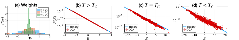
When we train the RBMs, our goal is to decrease the Kullback-Leibler divergence between training data’s distribution and the model’s distribution. To achieve this, one need to estimate the model’s distribution using Monte Carlo sampling. At this point, diabatic quantum annealing can be used. With the speed corresponds to , the sampled results would be not the ground state but the Boltzmann distribution at . According to the characteristics of the data used to train the RBMs, the deviations of the components of the weight matrix are different as shown in Fig. 1(d). We do not discuss this, but concentrate on the fact that qualities of the DQA are dependent to the deviation of the deviation. When high temperature Ising model (i.e. disordered data) used, the deviation of the matrix components is small, makes the DQA quality very high as shown in Fig. 1(c). Conversely, when low temperature Ising data (i.e. ordered data) are used, the deviation of the weight matrix was large, makes the DQA quality not good, but still hold the tendency following the Boltzmann distribution as shown in Fig. 1(a).
So far, a former study already tried to utilize quantum annealing to train the RBMs [3]. However, the sampling result of quantum annealing is supposed to be the Boltzmann sampling of , which means, only ground state is the original target of the sampling process. Of course the hardware systems of D-wave corporation are not yet perfect, the sampling results contain a few excited states making the distribution closer to a low temperature Boltzmann distribution. However, it is closer to a coincidence rather than a logical conclusion.
IV Comparison between the estimated distribution and the Boltzmann distribution
We calculate the Kullback–Leibler divergence(KL divergence) for several well-known models to confirm how the estimated distribution is similar to the Boltzmann distribution. The KL divergence represents how one distribution is different from the true distribution, which is written by
| (7) |
We simulate the quantum annealing with problem Hamiltonians as representative models composed of the two-dimensional Ising model and all-to-all Ising model. The Hamiltonian of all-to-all Ising model is written as
| (8) |
which has a critical point at . Since the all-to-all Ising model satisfies the mean-field theory, we introduce the two-dimensional Ising model which does not follow the mean-field theory to confirm whether the mean-filed theory is significant for the quality of estimated distribution. The Hamiltonian of the two-dimensional Ising model is given by
| (9) |
for length square lattice with periodic condition. The critical point is known as
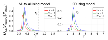
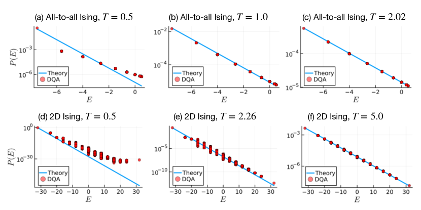
By numerical calculation of time ordered integral, Eq. (4), we prepare the estimated probability, , with different time gradient, , which have corresponding Boltzmann distribution, , with different . Fig. 2 provides the dependence of KL divergence on . They describes the Kullback-Leibler divergence between the target Boltzmann distribution and the estimated distribution. For paramagnetic phases, the KL divergences are very close to zero, while it is very high near critical point and low temperature regimes.
Fig. 2 shows the KL divergences between the theoretical boltzmann distributions and the estimated distribution using the DQA. Both the all-to-all Ising model and the 2D Ising model’s cases, the DQA is appreciable for high temperature regime, while near critical temperature and low temperature regime, it is not. Also, as the system sizes increases, the temperature that the DQA’s quality decrease increases.
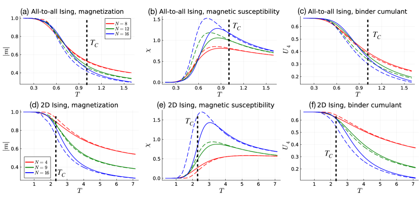
The quantum expectation value for an observable, , is given as . When the observable has the basis as , the quantum expectation value becomes, . The corresponding Boltzmann distribution has The thermal expectation given by for observable . Obviously, the deviation of the quantum expectation from the thermal expectation indicates how both distributions differ.
Fig. 4 shows the behaviors of the observables-magnetization, magnetic susceptibility and the binder cumulant. For both models, the differences between theoretical values and the estimated values using the DQA are maximum near critical temperature. Unlike the Fig. 2, the estimated values are very close to theoretical values at low temperature. This phenomenon is because at low temperatures, there is no state other than the ground state.
V Derivation of the effective temperature
Denoting by the -directional spin configuration, the problem Hamiltonian can generally be written as
| (10) |
Meanwhile, we can also write , where
| (11) |
represents the -spin interactions. Combining these two expressions, the energy of each can also be expressed as .
Expanding Eq. (4), the final state can be expressed as a Dyson series
| (12) |
where
| (13) |
For convenience, let us define . Since rotates each Pauli operator by the same amount, we can represent as
| (14) |
where .
Plugging Eq. (14) into Eq. (12) and using
| (15) |
we obtain
| (16) |
which yields the projective probability
| (17) |
We require that, up to order , this projective probability should be equal to the Boltzmann distribution
| (18) |
of modified Hamiltonian by first order of , where is given by
| (19) |
and the modifing factor is given by
| (20) |
We provided a linear function of with as the candidate of the schedule for the low-temperature Boltzmann sampling. Eq. (19) gives as
| (21) |
while the modifying factor is
| (22) |
when goes to infinity to satisfy the boundary condition, .
VI conclusion
In this study, we took a closer look at quantum annealing again. By modifying the schedule from adiabatic to diabatic linear process, namely diabatic quantum annealing, we showed analytically and numerically that the annealing speed is related to the specific temperature.
We firstly check how much different the estimated probabilistic distributions obtained by DQA process and the target theoretical distributions of the artificial neural networks. For various kinds of featured data sets, the DQA-estimated distributions are close to the Boltzmann distribution of the model. The deviation of the components of weight matrix is the key that determines the quality of DQA. As the deviations is smaller, the similarity between DQA estimated and the theoretical distribution are high.
Next, we check KL divergences between theoretical distributions and the DQA-estimated ones are very small for high temperature regime. However, from critical temperature to low temperature regime, the DQA’s quality seems to be not enough. A similar analysis is obtained for the observables of the Ising models. To summarize, the DQA-estimated distribution is very close when the effective temperature is high.
To summarize, effective temperature of the system is the key that determines the quality of the DQA. Particularly, when a artificial neural network system is in lazy learning regime [6], the sizes of the weight matrix would be small and hardly changes, the DQA’s estimation will be a good alternative to the conventional learning algorithm. Another case that the DQA would work well is when the system has very strong regularization condition.
All we have checked are linear schedule based DQA. We leave the exploration of various general schedules as future work.
Acknowledgements.
This work was supported by the Global-LAMP Program of the National Research Foundation of Korea (NRF) grant funded by the Ministry of Education (No. RS-2023-00301976).References
- Kadowaki and Nishimori [1998] T. Kadowaki and H. Nishimori, Quantum annealing in the transverse ising model, Phys. Rev. E 58, 5355 (1998).
- Raymond et al. [2016] J. Raymond, S. Yarkoni, and E. Andriyash, Global warming: Temperature estimation in annealers, Frontiers in ICT 3, 10.3389/fict.2016.00023 (2016).
- Pochart et al. [2022] T. Pochart, P. Jacquot, and J. Mikael, On the challenges of using d-wave computers to sample boltzmann random variables, in 2022 IEEE 19th international conference on software architecture companion (ICSA-C) (IEEE, 2022) pp. 137–140.
- Sandt and Spatschek [2023] R. Sandt and R. Spatschek, Efficient low temperature monte carlo sampling using quantum annealing, Scientific Reports 13, 6754 (2023).
- [5] https://www.dwavesys.com/.
- Geiger et al. [2020] M. Geiger, S. Spigler, A. Jacot, and M. Wyart, Disentangling feature and lazy training in deep neural networks, Journal of Statistical Mechanics: Theory and Experiment 2020, 113301 (2020).