RT-GuIDE: Real-Time Gaussian splatting for Information-Driven Exploration

Abstract

We propose a framework for active mapping and exploration that leverages Gaussian splatting for constructing information-rich maps. Further, we develop a parallelized motion planning algorithm that can exploit the Gaussian map for real-time navigation. The Gaussian map constructed onboard the robot is optimized for both photometric and geometric quality while enabling real-time situational awareness for autonomy. We show through simulation experiments that our method is competitive with approaches that use alternate information gain metrics, while being orders of magnitude faster to compute. In real-world experiments, our algorithm achieves better map quality (10% higher Peak Signal-to-Noise Ratio (PSNR) and 30% higher geometric reconstruction accuracy) than Gaussian maps constructed by traditional exploration baselines. Experiment videos and more details can be found on our project page: https://tyuezhan.github.io/RT_GuIDE/

I Introduction

Active mapping is a problem of optimizing the trajectory of an autonomous robot in an unknown environment to construct an informative map in real-time. It is a critical component of numerous real-world applications such as precision agriculture [1], infrastructure inspection [2], and search and rescue [3] missions. While nearly all tasks rely on recovering accurate metric information to enable path planning, many also require more fine-grained information. Recent advances in learned map representations from the computer vision and graphics communities [4, 5] have opened up new possibilities for active mapping and exploration while maintaining both geometrically and visually accurate digital twins of the environment.

While prior work effectively solves the problem of information-driven exploration [6, 7, 8, 9, 10] or frontier-based exploration [11, 12, 13], in this work we consider the additional problem of generating radiance fields while also performing autonomous navigation. Prior work has also proposed information metrics using novel learned scene representations that are capable of high quality visual reconstruction but are incapable of running in real-time onboard a robot. To enable efficient mapping and planning in these novel representations, we consider approximation techniques for computing the information gain. Further, we consider the problem of generating high-quality maps that are capable of novel-view synthesis that can be used for downstream applications.

Fig. 1 shows the elements of our approach. We use the Gaussian splatting approach proposed in [14] to generate Gaussian maps. We propose a novel information gain metric to compute the utility of regions in the environment and use a hierarchical planning framework to plan high-level navigation targets that yield maximal information in the environment and low-level paths that are dynamically feasible, collision-free and maximize the local information of the path. Our system runs real-time onboard a fully autonomous unmanned ground vehicle (UGV) to explore an unknown environment while generating a high-fidelity visual representation of the environment.

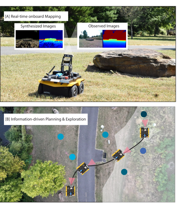
Figure 1: Key elements of our proposed approach. [A] Robot building a Gaussian map onboard in real-time and using it to avoid obstacles in the environment. Synthesized color and depth images from the Gaussian map are presented next to the corresponding observations from the RGBD sensor. [B] Robot navigating to unobserved areas (right) with high information gain while maximizing information along the trajectory. Gaussian frontiers colored cyan (light to dark) in increasing estimated information gain.

In summary, the contributions of this paper are:

1. A unified framework for online mapping and planning with Gaussians.

2. An approximate information gain metric that is easy to compute and capable of running in real-time onboard an unmanned ground vehicle.

3. A method to compute frontiers in a map built using Gaussian splatting.

4. Extensive experiments in both indoor and outdoor environments to evaluate our framework.

II Related Work

Map Representation. To effectively construct a map of the environment, numerous map representations have been proposed in the robotics community. The most intuitive but effective volumetric representation has been widely used. Voxel-based representation could maintain information such as occupancy [15] or signed distance [16, 17]. With the recent application of semantic segmentation, semantic maps that contain actionable information have been proposed [18, 19, 20, 21, 22]. With the recent advances in learned map representations in the computer vision community, Neural Radiance Fields (NeRF) [4] and 3D Gaussian Splatting (3DGS) [5] have become popular representations for robotic motion planning. In this work, we study the problem of active mapping with the learned map representations.

Active Simultaneous Localization and Mapping (SLAM). The problem of exploration and active SLAM has been widely studied in the past decade. The classical exploration framework uses a model-based approach to actively navigate towards frontiers [11, 12] or waypoints that have the highest information gain [6, 7, 8, 9, 10, 23, 24]. Some recent work combines the idea of frontier exploration and the information-driven approach to further improve efficiency [25, 26, 27, 28]. However, most of the existing work developed their approaches based on classical map representations. For example, frontiers are typically defined in voxel maps, information metrics are typically associated with occupancy maps or Signed Distance Field (SDF) maps.

In this work, we instead consider the active mapping problem with a learned map representation. Bayesian neural networks [29, 30] and deep ensembles [24, 31] are common approaches for estimating uncertainty in learned representations. [32, 33] use the idea of computing the uncertainty based on consecutive measurements from a moving robot in contrast to train multiple models in the traditional ensemble frameworks. Radiance field representations provide additional possibilities for estimating uncertainty through the volumetric rendering process [34]. [35] uses the difference between rendered depth and observations, and the alignment of $\alpha$-blended and median depth as measures of uncertainty.  [36] leverages Fisher information to compute pixel-wise uncertainty on rendered images. Where prior work in implicit and radiance field representations necessitates use indirect methods like ensembles and rendering for estimating uncertainty in the representation, a Gaussian map representation encodes physical parameters of the scene, which motivates estimating information gain from the Gaussians directly.

Navigation in Radiance Fields. Prior work has also considered planning directly in radiance fields. [37] plans trajectories in a Gaussian map and uses observability coverage and reconstruction loss stored in a voxel grid as an approximation of information gain for exploration. Sim-to-real approaches leverage the rendering quality of the learnt radiance fields to train downstream tasks such as visual localization, imitation learning [38] by effectively utilizing the representation as a simulator. [39] use a liquid neural network to train imitation policies for a quadrotor robot in a Gaussian splat. [40] utilize the geometric fidelity of the representation to first map the environment and then perform trajectory optimization to plan paths in these environments. [41] use a pre-generated Gaussian map to compute safe polytopes to generate paths and also present a method to synthesize novel views with a coarse localization of the robot and refine the estimate by solving a Perspective-n-Point (PnP) problem. The probabilistic representations of free space has also been utilized for motion planning [42] where authors use uncertainties in the learned representation to provide probabilistic guarantees on collision-free paths.

III Problem Specification

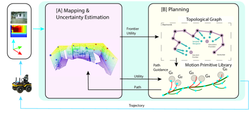
Figure 2: The proposed active mapping framework. The proposed framework contains two major components, the planning module and the mapping module. As can be seen in the figure, the Mapping module ([A]) takes in RGB, depth and pose measurements, and updates the map representation $m$ at every step and computes the utility of geometrically clustered frontiers. The information is then passed to the planning module which comprises the topological graph and motion primitive library ([B]). The topological graph adds sampled viewpoints as nodes and passes along a planned path to the trajectory planner. The trajectory planner in turn attempts to plan a path to goal that maximizes information gathering (queried from the mapper). The planned trajectory is executed by the robot to get a new set of observations.

We have an unknown map of the environment $m^{*}$ that belongs to a space of maps $\mathcal{M}$. Our goal is to solve the following problem

Problem 1.

Information-Driven Exploration.

$$\min_{x_{1:T}} \ \mathbb{E}_{x}[\rho(h(x,\hat{m}),h(x,m^{*}))]$$ (1)

$$s.t \ \hat{m}=\Phi(y_{1:T},x_{1:T})$$

$$\ y_{t}=h(x_{t},m^{*})\ \forall 1\leq t\leq T.$$

In the equation above, the expectation is taken over a random evaluation point $x$. The states belong to the state space $\mathcal{X}$, whereas observations belong to the observation space $\mathcal{Y}$. The observation function $h:\mathcal{X}\times\mathcal{M}\rightarrow\mathcal{Y}$ takes as input the robot state together with the map of the environment, and outputs the rendered image. $T$ represents the exploration budget. $m^{*}$ is the true map of the environment. $\hat{m}$ is the map of the environment that is estimated from the sequence of measurements $(y_{t})_{1\leq t\leq T}$ taken from vantage points (states) $(x_{t})_{1\leq t\leq T}.$ The discrepancy function $\rho$ captures the difference between the image rendered based on the estimated map, and the actual map. The sequence of vantage points is constrained to lie in free space $\mathcal{X}_{free}$.

Since Prob (1) is parameterized by $m^{*}$, which is a priori unknown, the problem is ill-posed. We are instead interested in synthesizing a (near) optimal policy $(\pi_{t})_{t=0}^{T}$, consisting of a sequence of functions that map the history of observations to the optimal action to take at the current step. In particular, for any $i\leq T$, the function

$$\pi_{t}:\mathcal{Y}_{1}\times\cdots\times\mathcal{Y}_{t} \rightarrow\mathcal{X}$$ (2)

$$\pi_{t}(y_{1},y_{2},...,y_{t}) =x_{t}$$

ought to specify the next vantage point given the the history of observations accrued thus far. Finding the optimal sequence of policies is a challenging, high-dimensional, optimization problem. We therefore develop an approximate method for solving it. The approximation lies in a particular, but suitable, choice of representation for $m^{*}$, together with a way of using it for effective exploration.

IV Method

Our proposed framework comprises the mapping module and the planning module, as illustrated in Fig. 2. The mapping module (Sec. IV-A) accumulates measurements and poses to generate a reconstruction of the environment and computes the utility of Gaussian frontiers. The information is then passed to the planning module for planning guidance paths (Sec. IV-B1) and trajectories (Sec. IV-B2).

IV-A Mapping & Uncertainty Estimation

IV-A1 Mapping

We adopt the 3D Gaussian Splatting (3DGS) approach to represent the environment as a map of 3D Gaussians. 3DGS enables real-time radiance field rendering by projecting and blending the 3D Gaussians to render images. The parameters of the 3D Gaussians are optimized through mapping iterations to improve the representation of the scene. We build the 3DGS mapping module upon the [14] framework. The poses of the robot are obtained using [43].

IV-A2 Gaussian uncertainty for viewpoint selection

We estimate uncertainty in the map representation directly on the 3D Gaussians. We motivate our metric of information gain leveraging the theory of Kalman filtering. In particular, the updates of the Kalman filter [44] are given by

$$m_{k|k} =m_{k|k-1}+K(y_{k}-Hx_{k|k-1})$$ (3)

$$K =P_{k|k-1}H^{T}S^{-1}$$

$$S =HP_{k|k-1}H^{T}+R$$

$$P_{k|k} =P_{k|k-1}-KHP_{k|k-1}.$$

where $K$ is the Kalman Gain, $P$ is the covariance of the map, $H$ is the linearized measurement model, $S$ is the innovation covariance and $R$ is the covariance of the measurement noise. The following identity holds:

$$Cov_{k|k-1}(m_{k|k}-m_{k|k-1})=P_{k|k-1}-P_{k|k}$$ (4)

The pertinent aspect of the relation above is that the prior covariance of the change in the map parameters upon observing a new measurement is equal to the information gain of the latter. Although this argument can be rigorously shown in the context of linear measurement models, we nevertheless use it as a measure of future information gain in the context of measurements with a Gaussian representation of the environment.

Gaussian uncertainty. Following the above motivation, we compute the change in Gaussian parameters across each mapping optimization and use the magnitude of the parameter updates $\|\hat{m}_{t}-\hat{m}_{t-1}\|$ as a measure of uncertainty. Gaussians with large changes in parameters represent parts of the scene with high uncertainty and conversely Gaussians with stable parameters have low uncertainty. We use this to approximate information gain for viewpoint selection.

Given a map $m$ represented by a set of Gaussians $G$, we classify the Gaussians in the scene $G=\{G_{H},G_{L},G_{O}\}$ into three disjoint subsets, $G_{H}$ which consists of Gaussians with high uncertainty, $G_{L}$ which consists of Gaussians with low uncertainty and $G_{O}$ for the rest. For a Gaussian $g_{i}\in G$ and pose $x_{t}$ at timestep $t$, we define the binary visibility function $v(x_{t},g_{i})$ capturing whether $g_{i}$ is in the field of view of $x_{t}$.

To maximize information gain while exploring the environment, we aim to find the viewpoint with the highest utility $\xi(x_{t})$ that maximizes the number of high-uncertainty Gaussians and minimizes the number of low-uncertainty Gaussians in the field of view at each timestep. The first term in Equ. 5 encourages observations of parts of the scene with high uncertainty while the second term encourages exploration of unseen areas of the scene. The balance of exploitation and exploration is weighted by the term $\lambda_{\xi}$.

$$\xi(x_{t})=\sum_{i\in L}v(x_{t},g_{i})-\lambda_{\xi}\sum_{i\in H}v(x_{t},g_{i})$$ (5)

Gaussian frontiers. In contrast to traditional mapping representations, the Gaussian map does not encode occluded and free space. Instead of frontiers of unobserved regions, we use the Gaussian uncertainty estimates to identify regions of the map that should be visited next, since Gaussians that have few observations or lie at the edges of observed regions naturally have higher uncertainty. For a region $o\subset m$, we consider the set of Gaussians $\{g\sim\mathcal{N}(\mu,\sigma^{2})\in G\ |\ \mu\in o\}$ with cardinality $N_{g}$ in the region and compute the mean uncertainty of that frontier

$$\Omega=\frac{1}{N_{g}}\sum^{N_{g}}_{i}\|\mu^{t}_{i}-\mu^{t-1}_{i}\|.$$ (6)

This provides a unified framework for estimating information gain to optimize map quality while implicitly identifying frontiers to guide the exploration of unknown regions.

IV-A3 Traversable region segmentation

We found Gaussians on the ground plane to be particularly noisy in indoor environments due to reflections off the floor. This necessitated the removal of Gaussians on the ground for planning. This also fulfilled an important role in reducing the number of Gaussians that have to be queried in the collision check.

IV-B Hierarchical Planning

We represent the planning problem as a hierarchical planning problem. The first level provides guidance to map particular regions of the environment and a path to that region from the known space in the environment. The second level finds a trajectory that is dynamically-feasible (i.e. obeys the robot’s physical constraints); collision-free and locally maximizes the information along the path.

IV-B1 High-level guidance

We formulate a high-level guidance path that allows us to (i) plan to transition to high uncertainty regions of space which might involve traveling through those with low uncertainty; and (ii) estimate the traversable space in the known space without explicitly having to plan long-range trajectories with computationally expensive collision checks. At the higher level of our planner, we construct a graph $\mathcal{G}(N,E)$ by incrementally adding nodes along the traveled path. The graph consists of two types of nodes $n_{o},n_{p}$ where $n_{o}$ are observed nodes (along our odometry) and $n_{p}$ are predicted nodes. At each planning iteration, we sample a fixed number of viewpoints around the identified regions. We can compute the shortest viewing distance from the Gaussian frontier $f\in\mathbb{R}^{3}$ to the optical center of the camera as

$$d_{1}=\frac{||f^{T}\left[b_{1}\ b_{2}\right]||_{2}}{tan\left(\phi/2\right)}$$

where $b$ is the camera axis and $\phi$ is the field of view of the camera. Each sampled viewpoint is then assigned the utility computed by the Gaussian frontiers and connected to the closest point in the graph. We then use Dijkstra’s search algorithm to find the shortest path from the current robot location in the graph to all the predicted nodes in the graph. We then compute the cost-benefit of a path using $\Omega/e^{d_{2}}$ where $\Omega$ is the estimated information gain and $d_{2}$ is the distance to the node [45]. The maximal cost-benefit path is sent to the trajectory planner.

IV-B2 Trajectory Generation

The second level planning problem involves finding a collision-free trajectory from start to goal that meets the dynamic constraints of the robot while optimizing the information along the path. The problem is defined as follows:

Problem 2.

Trajectory Planning. Given an initial robot state $x_{0}\in\mathcal{X}_{free}$, and goal region $\mathcal{X}_{goal}$, find the control inputs $u(\cdot)$ defined on $[0,\tau]$ that solve:

$$\min_{u(\cdot),\tau}\ J(u(\cdot),\tau)$$ (7)

$$s.t.\ \text{for all }t\in[0,\tau]$$

$$\dot{x}(t)=f(x(t),u(t)),\ x(t)\in\mathcal{X}_{free},$$

$$||v(t)||_{2}\leq v_{max},\ |\omega(t)|\leq\omega_{max},$$

$$x(0),\theta(0)=x_{0},\theta_{0},\ x(\tau)\in\mathcal{X}_{goal}$$

where $J$ is a function that encodes a positive combination of execution time $\tau$ and the control effort $J_{c}(u(\cdot))$.

We use the unicycle model as the robot dynamics. The robot state $x=[p,\theta]\in\mathbb{R}^{2}\times S^{1}$ consists of its position ($p$) and heading ($\theta$). The control inputs $u=[v,\omega]\in\mathbb{R}^{2}$ consist of linear velocity ($v$) and angular velocity $(\omega)$. Inspired by [46], we solve problem 2 by performing a tree search on the motion primitives tree. Motion primitives are generated with fixed control inputs over a time interval $\delta\tau$ with known initial states. Given the actuation constraints $v_{max}$ and $\omega_{max}$ of the robot, we uniformly generate $N_{v}\times N_{\omega}$ samples from $[0,v_{max}]\times[-\omega_{max},\omega_{max}]$ as the finite set of control inputs. Subsequently, motion primitives are constructed given the dynamics model, the controls $u$, and time discretization $d\tau$.

We sample a fixed number of points on each motion primitive to conduct collision checks. Since we have an uncertain map, we relax $x\in X_{free}$, to a chance constraint. First, we measure the distance from the discretized positions

$$w\sim\mathcal{N}(\kappa,r_{robot}^{2})\in W|\kappa=x_{t}$$

along the search path to all Gaussians

$$\{g\sim\mathcal{N}(\mu,\sigma^{2})\in G\}$$

in the map. Our constraint then boils down to the probability of the distance between the test point and the set of Gaussians in the scene

$$d_{g}=\inf||W-G||$$

being less than 0 i.e. $P(d_{g}<0)\leq\eta$ where $\eta$ is the tolerable risk. When checking for collisions, each sampled point is bounded with a sphere of radius $r_{robot}$ and the radius $\sigma$ of each Gaussian is scaled by a factor of $\lambda_{g}$. The truth value of the test is determined by comparing the distance to the closest Gaussian with $r_{robot}+\lambda_{g}\sigma$, as illustrated in Fig. 2. The rationale for the latter test is as follows. Assuming that the closest obstacle is unique, the probability of collision with some obstacle is well-approximated by the probability of collision with the nearest obstacle. This holds by virtue of the exponential decay of the Gaussian distribution with the distance from the origin. As a result, specifying an upper bound on the probability of collision is approximately the same as specifying the probability of collision with the closest obstacle.

We develop a GPU-accelerated approach for testing all sampled points with all Gaussians from the map at once while growing the search tree. This allows the real-time expansion of the search tree. The cost of each valid motion primitive is defined as

$$J(u(\cdot),\tau):=\lambda_{t}\tau+(v^{2}+w^{2})\tau,$$

where $\lambda_{t}$ weights the time cost with the control efforts. Since the maximum velocity of the robot is bounded by $v_{max}$, we consider the minimum time heuristic as

$$h(p):=||p_{goal}-p||_{2}/v_{max}.$$

We use A* to search through the motion primitives tree and keep top $k$ candidate trajectories for the subsequent information maximization. The information of each trajectory is evaluated with state sequence $[x(\delta\tau),\ldots,x(\tau)]$ on the trajectory according to (5). Finally, the trajectory with the highest information $\left(\sum_{t=0}^{\tau}\xi(x(t))\right)$ is selected and executed by the robot.

IV-C Implementation Details

We implemented the proposed method using PyTorch2.4. Most of our parameters of the Gaussian map were set to the default configuration of [14] for the TUM dataset. For simulation experiments, we used 50 mapping iterations. For real-world experiments, to enable real-time mapping and collision avoidance, we reduced the number of mapping iterations to 10 and pruned Gaussians once per mapping sequence. The mapping module ran at 1Hz and the planning module ran at 3Hz onboard the robot. We set Gaussian frontier size to 2.5m, $\lambda_{\xi}=1$ and $\lambda_{g}=3$.

V Simulation Results & Ablations

Table I: Simulation Results on 120 iTHOR scenes with 20 steps

Methods	PSNR $\uparrow$	SSIM $\uparrow$	LPIPS $\downarrow$	RMSE $\downarrow$	t/step $\downarrow$
	[dB]			[m]	[s]
Ensemble	12.589	0.483	0.612	1.064	11.094
FisherRF	13.702	0.558	0.549	1.016	5.347
Ours	13.591	0.533	0.576	0.975	0.046

Environments. We conduct simulation experiments with the AI2-THOR simulator [47] on the iTHOR dataset. The iTHOR dataset consists of indoor scenes including kitchens, bedrooms, bathrooms and living rooms.

Evaluation metrics & Baselines. For each scene, we generate a test set of images and evaluate the rendered images from each method against the test set. We evaluate the Peak Signal-to-Noise Ratio (PSNR), Structural Similarity Index (SSIM) [48], Learned Perceptual Image Patch Similarity (LPIPS) [49] on the RGB images and Root Mean-Square-Error (RMSE) on the depth images.

We evaluate the proposed information gain metric against two other view selection methods. For the Ensemble baseline, we train an ensemble of $5$ models with the leave-one-out procedure at each step. We compute the patch-wise variance across the rendered images for each sampled viewpoint and ensemble model, and select the viewpoint with the highest variance as the next action. For FisherRF, we follow the original implementation to evaluate viewpoints based on the Fisher information.

Experiments and results. In our simulation experiments, we set the grid size of reachable positions to 0.25m. At each step, we sample viewpoints with different yaw angles around the current position of the agent as possible actions to take. These viewpoints are then evaluated with the corresponding uncertainty metric and the viewpoint with the highest uncertainty is selected as the next action. We ran experiments on all 120 scenes from iTHOR with 20 steps each. We synthesized novel views according to the test set poses and computed the image metrics against the test set images.

The averaged results are presented in Tab. I. Our information gain metric performs comparably with FisherRF and

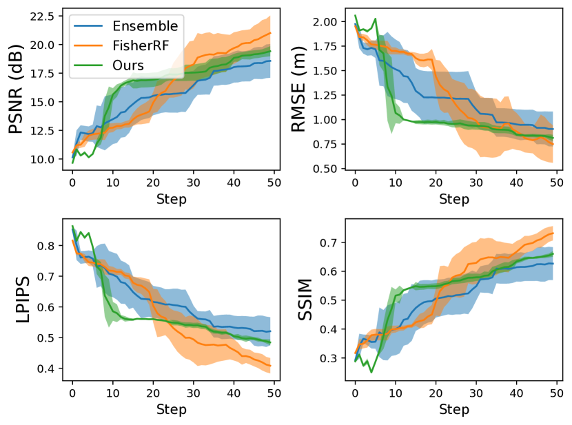
Figure 3: Comparison of viewpoint selection methods on environment FloorPlan7 of the iTHOR dataset with 50 steps. The average and variance are computed across 5 different seeds. Our proposed method achieves comparable performance to the other methods while exhibiting significantly smaller variance across runs.

outperforms Ensemble across all metrics, while being more than an order of magnitude faster in computation time. Since we are computing the uncertainty directly on the Gaussians instead of the image, we avoid the computation cost of rendering every sampled viewpoint. This efficiency in computation is crucial in a sampling-based planner where we evaluate potentially hundreds of viewpoints in each planning iteration. We also compute the mean and variance of the evaluation metrics across 50 steps for 5 different seeds, presented in Fig. 3. We note that our method exhibits significantly lower variance than the baselines. The simulations were run on a desktop computer with an AMD Ryzen Threadripper PRO 5975WX and NVIDIA RTX A4000 (16GB).

VI Real-world Experiments and Benchmark

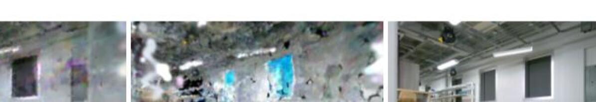
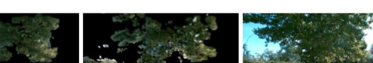
Figure 4: A qualitative comparison of the novel views rendered using the map generated by our method, onboard and in real-time, to the baseline and the ground truth. The first row is the rendered color images and the second row is the depth images.

Table II: Quantitative Results of Real-world Experiments.

Methods	Env.	PSNR [dB] $\uparrow$	SSIM $\uparrow$	LPIPS $\downarrow$	RMSE [m] $\downarrow$	mIoUa $\uparrow$	Traj. Len. [m]	Volume Mappedb [%]
Baseline-Voxel	Indoor	—	—	—	1.687	—	123.9	99.94
Baseline-GS		12.79	0.463	0.481	0.548	0.259	123.9	99.94
Ours-Budget	171$m^{2}$	13.52	0.512	0.462	0.503	0.273	123.9	98.94
Ours		13.88	0.534	0.442	0.449	0.290	179.1	100.0
Baseline-Voxel	Outdoor	—	—	—	0.965	—	159.9	100.0
Baseline-GS		14.17	0.678	0.406	0.718	0.282	159.9	100.0
Ours-Budget	460$m^{2}$	14.61	0.666	0.419	0.836	0.276	159.9	89.27
Ours		15.66	0.709	0.368	0.513	0.380	225.2	95.53
a Indoor classes: [floor, chair, table, refrigerator, trashcan]. Outdoor classes: [ground, tree, lamppost, rock, signboard, bench].
b Indoor Volume: 360.0m3. Outdoor Volume: 818.6m3.

VI-A Baselines & Experimental Setup

For a meaningful comparison, we implement a frontier-based exploration algorithm presented in [11] as a baseline method. It uses a 3D voxel map to represent the environment, detect frontiers, and generate plans to the nearest frontier. To improve the performance of the baseline method, we incorporated viewpoint sampling at frontier clusters presented in [27] and used A* to provide a reference path to the frontier for the MPL planner.

We deployed our algorithm and the baseline in 2 different real-world environments for comparison on a Clearpath Jackal robot outfitted with AMD Ryzen 5 3600 and RTX 4000 Ada SFF. In addition, it is equipped with an Ouster OS1 LiDAR for state estimation and Intel Realsense D455 camera for mapping. For the baseline method, we set the voxel resolution to 5cm and limit the frontier cluster size to 10cm. For a fair comparison, the baseline method plans on the voxel map but also maintains a Gaussian map to preserve the quality of view synthesis. To generate the groundtruth data for evaluation, we teleoperated the robot to uniformly sample the environment. The Baseline-Voxel method constructs a voxel map and plans with it. The Baseline-GS method constructs a Gaussian map onboard the robot in addition to the voxel map. We set the budget of Ours-Budget to be the trajectory length of the baseline method. We also carried out experiments for our method with a larger budget.

VI-B Evaluation

Qualitative We evaluate the quality of the Gaussian maps that were constructed in real-time onboard the robot by synthesizing images with the test set poses. Samples of synthesized color images and depth images are presented in Fig. 4. Compared to the Gaussian maps constructed by the baseline method, our synthesized depth images capture the depth value closer to the ground truth images while the color images are sharper with more detail. The rendered views from our method at novel camera poses result in better performance of downstream tasks such as semantic segmentation, details are analyzed in the next section.

Metrics. We computed the same image metrics on the RGB and depth images as in the simulation experiments. We rendered 1000 novel views according to the groundtruth poses from the test set and compared them against the corresponding images. We constrained the budget for each method by the distance traveled. To evaluate the coverage of the environment, we computed the volume mapped from the voxel maps built by each method (in post-process for ours).

Results & Discussion. When the budget is set to the trajectory length of the baseline, our method performs comparably with Baseline-GS. When a larger exploration budget is allowed, the frontier baselines terminate early (since they have explored all available frontiers) but our method is able to significantly improve map reconstruction quality. We attribute this to the information gain metric which enables re-visiting of areas in the environment to further improve map quality. We note that Baseline-Voxel is not able to render RGB images since it does not encode color information and also performs poorly in depth rendering due to the discretization of the voxel map. This further motivates the use of a Gaussian map that contains color in addition to geometric information. Our method optimizes for image rendering quality while still achieving mapped volume comparable with the baseline which prioritizes coverage.

To verify the usefulness of the generated Gaussian map representation for downstream tasks in robotics, we also evaluate the rendered images from each method on the task of semantic segmentation. We used Grounded SAM 2 [50, 51, 52, 53, 54] to perform semantic segmentation on the rendered and groundtruth images and computed the mean Intersection over Union (mIoU). Our approach achieves better mIoU scores for both scenes, indicating higher fidelity of the rendered images.

VII Limitations and Future work

In this work, we present a framework for real-time active exploration and mapping compatible with Gaussian Splatting. In future work, we wish to explore the use of Gaussian opacities to consider occluded Gaussians and improve the uncertainty estimates. Another future direction is to consider semantic features together with the Gaussian maps to perform complex tasks in the environment like object search and represent dynamic scenes in our framework. In this work, we use LiDAR to provide odometry but in future work, we aim to formulate this entire framework using a single sensor.

References

- [1] X. Liu, S. W. Chen, G. V. Nardari, C. Qu, F. Cladera, C. J. Taylor, and V. Kumar, “Challenges and opportunities for autonomous micro-uavs in precision agriculture,” IEEE Micro, vol. 42, no. 1, pp. 61–68, 2022.
- [2] A. Bircher, M. S. Kamel, K. Alexis, H. Oleynikova, and R. Siegwart, “Receding horizon path planning for 3d exploration and surface inspection,” Autonomous Robots, vol. 42, 02 2018.
- [3] Y. Tian, K. Liu, K. Ok, L. Tran, D. Allen, N. Roy, and J. P. How, “Search and rescue under the forest canopy using multiple uavs,” The International Journal of Robotics Research, vol. 39, no. 10-11, pp. 1201–1221, 2020.
- [4] B. Mildenhall, P. P. Srinivasan, M. Tancik, J. T. Barron, R. Ramamoorthi, and R. Ng, “Nerf: Representing scenes as neural radiance fields for view synthesis,” Communications of the ACM, vol. 65, no. 1, pp. 99–106, 2021.
- [5] B. Kerbl, G. Kopanas, T. Leimkühler, and G. Drettakis, “3d gaussian splatting for real-time radiance field rendering,” ACM Transactions on Graphics, vol. 42, no. 4, pp. 1–14, 2023.
- [6] K. Saulnier, N. Atanasov, G. J. Pappas, and V. Kumar, “Information theoretic active exploration in signed distance fields,” in 2020 IEEE International Conference on Robotics and Automation (ICRA), 2020, pp. 4080–4085.
- [7] L. Schmid, M. Pantic, R. Khanna, L. Ott, R. Siegwart, and J. Nieto, “An efficient sampling-based method for online informative path planning in unknown environments,” IEEE Robotics and Automation Letters, vol. 5, no. 2, pp. 1500–1507, 2020.
- [8] B. Charrow, S. Liu, V. Kumar, and N. Michael, “Information-theoretic mapping using cauchy-schwarz quadratic mutual information,” in 2015 IEEE International Conference on Robotics and Automation (ICRA), 2015, pp. 4791–4798.
- [9] A. Bircher, M. Kamel, K. Alexis, H. Oleynikova, and R. Siegwart, “Receding horizon” next-best-view” planner for 3d exploration,” in 2016 IEEE international conference on robotics and automation (ICRA). IEEE, 2016, pp. 1462–1468.
- [10] M. Dharmadhikari, T. Dang, L. Solanka, J. Loje, H. Nguyen, N. Khedekar, and K. Alexis, “Motion primitives-based path planning for fast and agile exploration using aerial robots,” in 2020 IEEE International Conference on Robotics and Automation (ICRA), 2020, pp. 179–185.
- [11] B. Yamauchi, “A frontier-based approach for autonomous exploration,” in Proceedings 1997 IEEE International Symposium on Computational Intelligence in Robotics and Automation CIRA’97.’Towards New Computational Principles for Robotics and Automation’. IEEE, 1997, pp. 146–151.
- [12] S. Shen, N. Michael, and V. Kumar, “Autonomous indoor 3d exploration with a micro-aerial vehicle,” in 2012 IEEE international conference on robotics and automation. IEEE, 2012, pp. 9–15.
- [13] J. Yu, H. Shen, J. Xu, and T. Zhang, “Echo: An efficient heuristic viewpoint determination method on frontier-based autonomous exploration for quadrotors,” IEEE Robotics and Automation Letters, vol. 8, no. 8, pp. 5047–5054, 2023.
- [14] N. Keetha, J. Karhade, K. M. Jatavallabhula, G. Yang, S. Scherer, D. Ramanan, and J. Luiten, “Splatam: Splat, track & map 3d gaussians for dense rgb-d slam,” in Proceedings of the IEEE/CVF Conference on Computer Vision and Pattern Recognition, 2024.
- [15] A. Hornung, K. M. Wurm, M. Bennewitz, C. Stachniss, and W. Burgard, “Octomap: An efficient probabilistic 3d mapping framework based on octrees,” Autonomous robots, vol. 34, pp. 189–206, 2013.
- [16] L. Han, F. Gao, B. Zhou, and S. Shen, “Fiesta: Fast incremental euclidean distance fields for online motion planning of aerial robots,” in 2019 IEEE/RSJ International Conference on Intelligent Robots and Systems (IROS), 2019, pp. 4423–4430.
- [17] H. Oleynikova, Z. Taylor, M. Fehr, R. Siegwart, and J. Nieto, “Voxblox: Incremental 3d euclidean signed distance fields for on-board mav planning,” in 2017 IEEE/RSJ International Conference on Intelligent Robots and Systems (IROS), 2017, pp. 1366–1373.
- [18] S. Yang and S. Scherer, “CubeSLAM: Monocular 3-D object SLAM,” IEEE Transactions on Robotics, vol. 35, no. 4, pp. 925–938, 2019.
- [19] S. L. Bowman, N. Atanasov, K. Daniilidis, and G. J. Pappas, “Probabilistic data association for semantic SLAM,” in IEEE international conference on robotics and automation (ICRA). IEEE, 2017, pp. 1722–1729.
- [20] N. Hughes, Y. Chang, and L. Carlone, “Hydra: A real-time spatial perception system for 3D scene graph construction and optimization,” Robotics: Science and Systems XVIII, 2022.
- [21] A. Asgharivaskasi and N. Atanasov, “Semantic octree mapping and shannon mutual information computation for robot exploration,” IEEE Transactions on Robotics, vol. 39, no. 3, pp. 1910–1928, 2023.
- [22] X. Liu, J. Lei, A. Prabhu, Y. Tao, I. Spasojevic, P. Chaudhari, N. Atanasov, and V. Kumar, “Slideslam: Sparse, lightweight, decentralized metric-semantic slam for multi-robot navigation,” 2024. [Online]. Available: https://arxiv.org/abs/2406.17249
- [23] S. He, Y. Tao, I. Spasojevic, V. Kumar, and P. Chaudhari, “An active perception game for robust autonomous exploration,” 2024. [Online]. Available: https://arxiv.org/abs/2404.00769
- [24] S. He, C. D. Hsu, D. Ong, Y. S. Shao, and P. Chaudhari, “Active perception using neural radiance fields,” arXiv preprint arXiv:2310.09892, 2023.
- [25] A. Dai, S. Papatheodorou, N. Funk, D. Tzoumanikas, and S. Leutenegger, “Fast frontier-based information-driven autonomous exploration with an mav,” in 2020 IEEE International Conference on Robotics and Automation (ICRA), 2020, pp. 9570–9576.
- [26] B. Zhou, Y. Zhang, X. Chen, and S. Shen, “Fuel: Fast uav exploration using incremental frontier structure and hierarchical planning,” IEEE Robotics and Automation Letters, vol. 6, no. 2, pp. 779–786, 2021.
- [27] Y. Tao, Y. Wu, B. Li, F. Cladera, A. Zhou, D. Thakur, and V. Kumar, “SEER: Safe efficient exploration for aerial robots using learning to predict information gain,” in 2023 IEEE International Conference on Robotics and Automation (ICRA). IEEE, 2023, pp. 1235–1241.
- [28] Y. Tao, X. Liu, I. Spasojevic, S. Agarwal, and V. Kumar, “3d active metric-semantic slam,” IEEE Robotics and Automation Letters, vol. 9, no. 3, pp. 2989–2996, 2024.
- [29] X. Pan, Z. Lai, S. Song, and G. Huang, “Activenerf: Learning where to see with uncertainty estimation,” in European Conference on Computer Vision. Springer, 2022, pp. 230–246.
- [30] S. Lee, K. Kang, and H. Yu, “Bayesian nerf: Quantifying uncertainty with volume density in neural radiance fields,” arXiv preprint arXiv:2404.06727, 2024.
- [31] G. Georgakis, B. Bucher, A. Arapin, K. Schmeckpeper, N. Matni, and K. Daniilidis, “Uncertainty-driven planner for exploration and navigation,” in 2022 International Conference on Robotics and Automation (ICRA), 2022, pp. 11 295–11 302.
- [32] C. Liu, J. Gu, K. Kim, S. G. Narasimhan, and J. Kautz, “Neural rgb (r) d sensing: Depth and uncertainty from a video camera,” in Proceedings of the IEEE/CVF Conference on Computer Vision and Pattern Recognition, 2019, pp. 10 986–10 995.
- [33] S. Sudhakar, V. Sze, and S. Karaman, “Uncertainty from motion for dnn monocular depth estimation,” in 2022 International Conference on Robotics and Automation (ICRA). IEEE, 2022, pp. 8673–8679.
- [34] S. Lee, L. Chen, J. Wang, A. Liniger, S. Kumar, and F. Yu, “Uncertainty guided policy for active robotic 3d reconstruction using neural radiance fields,” IEEE Robotics and Automation Letters, vol. 7, no. 4, pp. 12 070–12 077, 2022.
- [35] J. Hu, X. Chen, B. Feng, G. Li, L. Yang, H. Bao, G. Zhang, and Z. Cui, “Cg-slam: Efficient dense rgb-d slam in a consistent uncertainty-aware 3d gaussian field,” 2024.
- [36] W. Jiang, B. Lei, and K. Daniilidis, “Fisherrf: Active view selection and uncertainty quantification for radiance fields using fisher information,” 2023. [Online]. Available: https://arxiv.org/abs/2311.17874
- [37] R. Jin, Y. Gao, Y. Wang, H. Lu, and F. Gao, “Gs-planner: A gaussian-splatting-based planning framework for active high-fidelity reconstruction,” 2024. [Online]. Available: https://arxiv.org/abs/2405.10142
- [38] V. Murali, G. Rosman, S. Karamn, and D. Rus, “Learning autonomous driving from aerial views,” in 2024 IEEE/RSJ international conference on intelligent robots and systems (IROS). IEEE, 2024.
- [39] A. Quach, M. Chahine, A. Amini, R. Hasani, and D. Rus, “Gaussian splatting to real world flight navigation transfer with liquid networks,” arXiv preprint arXiv:2406.15149, 2024.
- [40] M. Adamkiewicz, T. Chen, A. Caccavale, R. Gardner, P. Culbertson, J. Bohg, and M. Schwager, “Vision-only robot navigation in a neural radiance world,” IEEE Robotics and Automation Letters, vol. 7, no. 2, pp. 4606–4613, 2022.
- [41] T. Chen, O. Shorinwa, W. Zeng, J. Bruno, P. Dames, and M. Schwager, “Splat-nav: Safe real-time robot navigation in gaussian splatting maps,” arXiv preprint arXiv:2403.02751, 2024.
- [42] T. Chen, P. Culbertson, and M. Schwager, “Catnips: Collision avoidance through neural implicit probabilistic scenes,” IEEE Transactions on Robotics, vol. 40, pp. 2712–2728, 2024.
- [43] C. Bai, T. Xiao, Y. Chen, H. Wang, F. Zhang, and X. Gao, “Faster-lio: Lightweight tightly coupled lidar-inertial odometry using parallel sparse incremental voxels,” IEEE Robotics and Automation Letters, vol. 7, no. 2, pp. 4861–4868, 2022.
- [44] R. E. Kalman, “A new approach to linear filtering and prediction problems,” 1960.
- [45] C. Gomez, M. Fehr, A. Millane, A. C. Hernandez, J. Nieto, R. Barber, and R. Siegwart, “Hybrid topological and 3d dense mapping through autonomous exploration for large indoor environments,” in 2020 IEEE International Conference on Robotics and Automation (ICRA), 2020, pp. 9673–9679.
- [46] S. Liu, N. Atanasov, K. Mohta, and V. Kumar, “Search-based motion planning for quadrotors using linear quadratic minimum time control,” in 2017 IEEE/RSJ international conference on intelligent robots and systems (IROS). IEEE, 2017, pp. 2872–2879.
- [47] E. Kolve, R. Mottaghi, W. Han, E. VanderBilt, L. Weihs, A. Herrasti, M. Deitke, K. Ehsani, D. Gordon, Y. Zhu, et al., “Ai2-thor: An interactive 3d environment for visual ai,” arXiv preprint arXiv:1712.05474, 2017.
- [48] Z. Wang, E. Simoncelli, and A. Bovik, “Multiscale structural similarity for image quality assessment,” in The Thrity-Seventh Asilomar Conference on Signals, Systems & Computers, 2003, vol. 2, 2003, pp. 1398–1402 Vol.2.
- [49] R. Zhang, P. Isola, A. A. Efros, E. Shechtman, and O. Wang, “The unreasonable effectiveness of deep features as a perceptual metric,” in CVPR, 2018.
- [50] S. Liu, Z. Zeng, T. Ren, F. Li, H. Zhang, J. Yang, C. Li, J. Yang, H. Su, J. Zhu, et al., “Grounding dino: Marrying dino with grounded pre-training for open-set object detection,” arXiv preprint arXiv:2303.05499, 2023.
- [51] T. Ren, Q. Jiang, S. Liu, Z. Zeng, W. Liu, H. Gao, H. Huang, Z. Ma, X. Jiang, Y. Chen, Y. Xiong, H. Zhang, F. Li, P. Tang, K. Yu, and L. Zhang, “Grounding dino 1.5: Advance the ”edge” of open-set object detection,” 2024.
- [52] T. Ren, S. Liu, A. Zeng, J. Lin, K. Li, H. Cao, J. Chen, X. Huang, Y. Chen, F. Yan, Z. Zeng, H. Zhang, F. Li, J. Yang, H. Li, Q. Jiang, and L. Zhang, “Grounded sam: Assembling open-world models for diverse visual tasks,” 2024.
- [53] A. Kirillov, E. Mintun, N. Ravi, H. Mao, C. Rolland, L. Gustafson, T. Xiao, S. Whitehead, A. C. Berg, W.-Y. Lo, P. Dollár, and R. Girshick, “Segment anything,” arXiv:2304.02643, 2023.
- [54] Q. Jiang, F. Li, Z. Zeng, T. Ren, S. Liu, and L. Zhang, “T-rex2: Towards generic object detection via text-visual prompt synergy,” 2024.