Intruding the sealed land: Unique forbidden beta decays at zero momentum transfer
Abstract
We report the first study of the structure-dependent electromagnetic radiative corrections to unique first-forbidden nuclear beta decays. We show that the insertion of angular momentum into the nuclear matrix element by the virtual/real photon exchange opens up the decay at vanishing nuclear recoil momentum which was forbidden at tree level, leading to a dramatic change in the decay spectrum not anticipated in existing studies. We discuss its implications for precision tests on the Standard Model and searches for new physics.
The standard classification of nuclear beta decays follows angular momentum and parity selection rules. Consider the tree-level amplitude that depends on the nuclear matrix element:
| (1) |
where is the charged weak current, and , , denote the spin, parity, and momentum of the initial (final) nucleus. Decays that satisfy the selection rules: and are known as “allowed” beta decays, while the rest are known as “forbidden” decays as their tree-level transition matrix elements are kinematically suppressed. In particular, for decays with , the amplitude above survives only when the nuclear recoil momentum is non-zero, due to rotational invariance.
Allowed beta decays provide stringent tests of the Standard Model (SM) and probe physics beyond the Standard Model (BSM) [1], e.g. through the precise measurement of the Cabibbo-Kobayashi-Maskawa (CKM) matrix elements [2, 3], and by constraining exotic interactions [4, 5, 6, 7, 8, 9, 10, 11, 12, 13]. On the other hand, forbidden decays have recently received increased attention due to their complementary role in probing new physics [14], e.g. exotic (non -) charged-current couplings (see Refs. [4, 6] for a mapping between the traditional Lee-Yang [15] nucleon-level interaction and the modern Standard Model Effective Field theory framework). It has recently been highlighted that measurements of the unique forbidden beta decay spectrum provide simultaneous access to both the Fierz term and the electron-neutrino angular correlation [16, 17]; the former is linear in the coefficients of new physics but lacks sensitivity to right-handed neutrino interactions, while the latter is sensitive to both left- and right-handed neutrino interactions but is quadratic in the new physics coefficients. As an example, we consider the unique first forbidden decay (, ), whose leading order matrix element is suppressed linearly by the nuclear momentum transfer . The tree-level differential decay rate takes the form
| (2) |
where comes from the nuclear matrix element squared, () is the mass (energy) of the emitted electron, and . The observables depending on the BSM tensor coefficients [15, 18, 19] are the Fierz term , and the angular correlation . The last term multiplied by in the tree-level rate does not exist in allowed decays. This term prevents the angular correlation from vanishing as in the allowed decays when integrating over the angles, making the unique forbidden spectrum sensitive to , and as a result, also to right-handed tensor couplings.
This observation has motivated a number of new experiments to study unique first-forbidden decays. Measurements of 90SrY and 90YZr are currently being conducted at the Hebrew University of Jerusalem, and these will be followed with measurements of 16NO, with an aim for accuracy [20, 21, 22]. Additionally, studies on 90YZr and 144PrNd are underway at the Oak Ridge National Laboratory, aiming for 1-2% accuracy at the first stage [23, 24]. However, similar to their allowed counterparts, one requires all the SM predictions of the forbidden decays to reach the same accuracy in order to maximize the discovery potential of the experiments. Existing theory analyses of forbidden beta decays focus mainly on calculations of tree-level transition amplitudes, Coulomb effects, shape factor and recoil corrections [25, 26, 27, 28, 29, 30, 31, 32, 33, 34, 35, 36, 37, 38, 39, 40, 41, 42, 43, 44, 45, 46, 47, 48, 49, 50, 51, 52, 53, 54, 55, 56, 57, 58, 59]. Existing shell model calculations of tree-level matrix elements typically have uncertainties spanning an order of magnitude [29, 37, 49], which will be improved with future ab initio calculations, e.g. [60]. However, an important missing piece in the program is the study of the full one-loop radiative correction (RC) to the forbidden decay amplitude; the latter is known to play a central role in the interpretation of precision beta decays, e.g. the extraction of [61, 62, 63, 64, 65, 66, 67, 68, 69], the nucleon axial coupling constant [70, 71, 72, 73], and the correction to the beta spectrum [74, 75, 76].
In this Letter, we report the first study of the RC to forbidden decays which leads to an interesting new observation: The usual statement that forbidden decay amplitudes with vanish in the non-recoil limit is falsified by the RC due to the introduction of an extra current operator into the nuclear matrix element that alleviates the inhibition from the angular momentum difference. As a consequence, at small enough the RC amplitude actually overtakes Eq.(2) as the main contributor to the forbidden decay rate. The same effect can also be achieved with new light degrees of freedom (DOFs) in the BSM sector that take the role of the photon in the RC. Explicitly, the differential decay rate now takes the form:
| (3) |
where the first two terms probe the SM RC and light new physics, while the third term probes the SM tree-level effects and heavy new physics. Therefore, the precise study of the behavior of forbidden decays provides a unique opportunity to simultaneously probe higher-order SM physics as well as BSM physics, without being contaminated by the large SM tree-level uncertainty. We investigate this novel idea in detail and discuss future prospects.
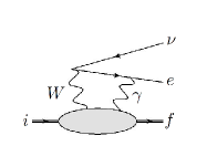
We begin by studying the SM RC. It can be recognized that among all the corrections, only the two diagrams in Fig.1, namely the -box diagram and the bremsstrahlung diagram with a photon emitted by the nucleus, can lead to a non-zero amplitude at , since all other diagrams depend on the tree-level nuclear matrix element in Eq.(1) (although may be renormalized) which has to satisfy the same angular momentum and parity selection rules. Their corresponding amplitudes read (assuming -decay) [64]:
| (4) |
where is the lepton current, and
| (5) |
is a “generalized Compton tensor” involving the electromagnetic () and weak () currents, with external momenta and . We focus on the -box diagram that gives the dominant contribution as we show later.
To be concrete, let us concentrate on unique first-forbidden decays involving the transition , in accordance with the planned experiments we mentioned in the introduction. The first important observation is that at the loop integral in is dominated by small values of the virtual photon momentum . This is seen by noticing that when is large, one may take in the integrand which reduces the integral to:
| (6) |
where
| (7) |
No matter how complicated is, it remains an ordinary four-vector with no external momentum dependence, so must vanish due to rotational invariance given that . Hence, the integral is dominated by the small- region, and more precisely the ultrasoft photon region in which (see Refs. [67, 68] for a discussion of radiative corrections to superallowed decays in terms of various regions in photon virtuality). In the ultrasoft region, the main contribution to is from nuclear ground- and excited states , which allows us to rewrite it as:
| (8) |
where we take and all states are normalized to 1.
In the small- region, we can take as a small expansion parameter, where and is a typical nuclear radius. This allows us to apply the standard multipole expansion of the Fourier-transformed current operators [77]:
| (9) |
where ; here we introduce , , , as the Coulomb, longitudinal, transverse magnetic and transverse electric multipole operators respectively, with the polarization vectors , defined in a coordinate frame with . Following the power counting in the multipole formalism, we find that the leading contributors to for the transition (here stands for ground state) involve the ground states and the excited states . While the full leading expression of can be found in the supplementary material, we observe that the ground state contribution involves the electromagnetic Coulomb operator and is enhanced by the atomic number . It gives rise to:
| (10) |
where the upper (lower) sign corresponds to the () decay, are reduced nuclear matrix elements (non-zero at ) defined in Table S I in the supplementary material, and is the magnetic quantum number of the external nuclear state along . The matrix (where ), whose explicit expression can be found in the supplementary material, is responsible for the rotation of the spin state along to that along ; the latter is needed for the proper application of the Wigner-Eckart theorem involving the multipole operators.
We may now evaluate the box diagram amplitude . First, to suppress the dependence on physics at large , we make use of our previous argument that the amplitude vanishes at to write the amplitude in the subtracted form
| (11) |
We then substitute the leading small- expression of given in Eq.(8) in the integrand appearing in both and . We may then evaluate the -integral by closing up the contour from the lower half in the complex -plane (which is an arbitrary choice; one may also choose the upper half). In doing so we observe that, only the residue at is enhanced by the atomic number at small ; picking up other poles always leads to a partial cancellation between the two elastic terms in Eq.(10), , that loses such an enhancement. It is also easy to see that the bremsstrahlung amplitude does not receive such an enhancement, because there the in does not play a role and the partial cancellation always takes place. Retaining only the -enhanced term 111Without an explicit calculation, one cannot exclude that the sum over the excited intermediate state may make up for the factor. However, even if this were the case, it is unlikely that such neglected terms exactly cancel the contribution we focus on here, absent a symmetry to enforce the cancellation. Moreover, in radiative corrections to other systems [69], no strong sensitivity to highly excited nuclear states is observed. leads to, after straightforward algebra:
| (12) |
where we are left with two scalar integrals:
| (13) |
where .
The above integrals are logarithmically divergent in the ultraviolet. In an effective field theory (EFT) approach, one would regulate the integrals in dimensional regularization and reabsorb the divergence through terms from the potential photon region [67]. Here, however, we are interested in a first rough estimate and therefore introduce the -dependence of and as a means to ensure the ultraviolet-finiteness of the -integral and obtain a model-dependent value for the corresponding EFT coupling. In principle, can be inferred from the nuclear charge distribution data and the latter requires nuclear structure calculations, but in this Letter we resort to a simple approximation for illustration. First, we know the small- expansion of the charge form factor: , where is the nuclear root-mean-square charge radius. So, we adopt a simple monopole expression for the charge form factor (with ) that reproduces the leading term in the small--expansion. We assume the same form factor in for simplicity:
| (14) |
since no extra information of the latter is currently available. With these, the integrals , can be evaluated analytically, and the squared amplitude as well as the tree-loop interference , after averaging and summing over initial and final spins, are found to be:
| (15) |
where 222Using dimensional regularization one obtains the same result with the replacement . The appearance of the angle in the second expression is because one needs to re-align the nuclear polarization direction in from to in order to interfere with in Eq.(12). Recall that the result above is derived by taking in , and the non-vanishing of demonstrates our assertion at the beginning of this Letter. Notice, however, that one still keeps the finite in the momentum conservation , and Eq.(15) may still be applicable for small but non-zero values of .
It is instructive to compare the radiative terms to the tree-level squared amplitude [16]:
| (16) |
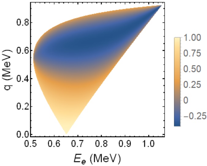
We do this for the transition 90SrY, which is interesting due to its large and a particularly small -value of 545.9(14) keV; fm is taken for the nuclear radius [80]. First, we plot the quantity in the full 3-body phase space () spanned by and :
| (17) |
where
| (18) |
with , and sums the three terms in Eqs.(15) and (16). From Fig.2 it is clearly seen that the size of the radiative corrections is substantial, and overtakes the tree-level contribution in the small- region which constitutes a significant portion of the entire phase space.
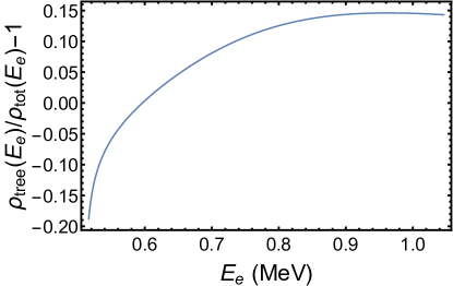
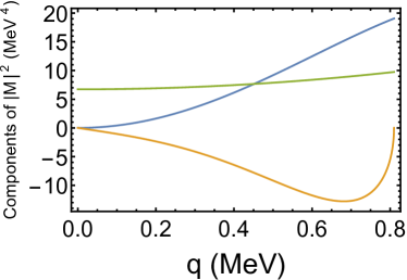
In Fig.3 we plot the various terms in Eqs.(15), (16)on a fixed-energy slice in the phase space: , that includes the point. One sees that, at the tree-level squared amplitude and the interference term decay as and respectively, while approaches a constant, which leads to its dominance at the small- region, in stark contrast to the traditional understanding of forbidden decays; therefore, any precision study of the decay shape without including the RC would be premature. We can also study the effect of RC on the total decay rate using the formula:
| (19) |
For 90SrY, we obtain , indicating a somewhat smaller correction to the total rate compared to the decay shape; this is due to a partial cancellation between the orange and green lines in Fig.3, which is purely accidental. One can also study the correction to the beta spectrum, as we present in the supplementary material. Notice that the -integrated results should be taken with a grain of salt as our approximate formula becomes inaccurate in the high- region. We defer the more comprehensive analysis at arbitrary to a later work.
In conclusion, we have shown that the existing understanding of decay kinematics in forbidden nuclear transitions has to be thoroughly revisited; the thought-to-be forbidden region of is opened up by RC, and depending on the specific transition the RC contribution may even be larger than the tree-level in a wider kinematic region. On the one hand, this imposes an extra challenge to the theory community due to the need to compute -dependent nuclear matrix elements, for instance , using reliable ab initio methods in order to correctly interpret forbidden beta decay data. On the other hand, our work also unveils a number of new experimental opportunities and discovery potential. By focusing on the small- region, one effectively evades the large tree-level uncertainty and has a direct experimental probe of the RC physics. It is also interesting to notice that, the topologies in Fig.1 that open up the forbidden decay at are not only achievable within the SM, but also with new physics. While modifications to the charged-current interactions induced by heavy new physics do not work [16], light new DOFs can play a similar role as the SM photon and open up the decay at . Therefore, forbidden decays at small provide a perfect avenue to study such light new DOFs, provided that the SM RC in this region is computed to a moderate accuracy. We hope these findings provide new motivations for future theoretical and experimental programs in this topic.
Acknowledgements.
We thank Oscar Naviliat-Cuncic, Mikhail Gorchtein, Leendert Hayen, Charlie Rasco and Guy Ron for inspiring discussions. C.-Y.S. and A.G.-M. are supported in part by the U.S. Department of Energy (DOE), Office of Science, Office of Nuclear Physics, under award DE-FG02-97ER41014. Additionally, C.-Y.S. receives support from the FRIB Theory Alliance award DE-SC0013617, and A.G.-M. is supported by the DOE Topical Collaboration "Nuclear Theory for New Physics", award No. DE-SC0023663, and the Hebrew University of Jerusalem through the Dalia and Dan Maydan Post-Doctoral Fellowship. V.C. is supported by the U.S. DOE Office of Science, Office of Nuclear Physics, under Grant No. DE-FG02-00ER41132.References
- Gorchtein and Seng [2024] M. Gorchtein and C. Y. Seng, Superallowed nuclear beta decays and precision tests of the Standard Model, Ann. Rev. Nucl. Part. Sci. 74, 23 (2024), arXiv:2311.00044 [nucl-th] .
- Cabibbo [1963] N. Cabibbo, Unitary Symmetry and Leptonic Decays, Meeting of the Italian School of Physics and Weak Interactions Bologna, Italy, April 26-28, 1984, Phys. Rev. Lett. 10, 531 (1963).
- Kobayashi and Maskawa [1973] M. Kobayashi and T. Maskawa, CP Violation in the Renormalizable Theory of Weak Interaction, Prog. Theor. Phys. 49, 652 (1973).
- Cirigliano et al. [2013a] V. Cirigliano, M. Gonzalez-Alonso, and M. L. Graesser, Non-standard Charged Current Interactions: beta decays versus the LHC, JHEP 02, 046, arXiv:1210.4553 [hep-ph] .
- Cirigliano et al. [2013b] V. Cirigliano, S. Gardner, and B. Holstein, Beta Decays and Non-Standard Interactions in the LHC Era, Prog. Part. Nucl. Phys. 71, 93 (2013b), arXiv:1303.6953 [hep-ph] .
- Gonzalez-Alonso et al. [2019] M. Gonzalez-Alonso, O. Naviliat-Cuncic, and N. Severijns, New physics searches in nuclear and neutron decay, Prog. Part. Nucl. Phys. 104, 165 (2019), arXiv:1803.08732 [hep-ph] .
- Cirigliano et al. [2023a] V. Cirigliano, W. Dekens, J. de Vries, E. Mereghetti, and T. Tong, Anomalies in global SMEFT analyses: a case study of first-row CKM unitarity, (2023a), arXiv:2311.00021 [hep-ph] .
- Johnson et al. [1963] C. H. Johnson, F. Pleasonton, and T. A. Carlson, Precision measurement of the recoil energy spectrum from the decay of , Phys. Rev. 132, 1149 (1963).
- Glück [1998] F. Glück, Order- radiative correction to 6he and 32ar decay recoil spectra, Nucl. Phys. A 628, 493 (1998).
- Glick-Magid et al. [2022] A. Glick-Magid, C. Forssén, D. Gazda, D. Gazit, P. Gysbers, and P. Navrátil, Nuclear ab initio calculations of 6he -decay for beyond the standard model studies, Phys. Lett. B 832, 137259 (2022).
- Müller et al. [2022] P. Müller, Y. Bagdasarova, R. Hong, A. Leredde, K. Bailey, X. Fléchard, A. García, B. Graner, A. Knecht, O. Naviliat-Cuncic, et al., -nuclear-recoil correlation from he 6 decay in a laser trap, Phys. Rev. Lett. 129, 182502 (2022).
- Mishnayot et al. [4355] Y. Mishnayot, A. Glick-Magid, H. Rahangdale, M. Hass, B. Ohayon, A. Gallant, N. D. Scielzo, S. Vaintraub, R. O. Hughes, T. Hirsch, C. Forssén, D. Gazda, P. Gysbers, J. Menéndez, P. Navrátil, L. Weissman, V. Srivastava, A. Kreisel, B. Kaizer, H. Dafna, M. Buzaglo, D. Gazit, J. T. Harke, and G. Ron, Constraining new physics with a measurement of the 23Ne -decay branching ratio 10.48550/arxiv.2107.14355 (arXiv:2107.14355).
- Longfellow et al. [2024] B. Longfellow, A. Gallant, G. Sargsyan, M. Burkey, T. Hirsh, G. Savard, N. Scielzo, L. Varriano, M. Brodeur, D. Burdette, et al., Improved tensor current limit from b 8 decay including new recoil-order calculations, Phys. Rev. Lett. 132, 142502 (2024).
- Brodeur et al. [2023] M. Brodeur, N. Buzinsky, M. A. Caprio, V. Cirigliano, J. A. Clark, P. J. Fasano, J. A. Formaggio, A. T. Gallant, A. Garcia, S. Gandolfi, S. Gardner, A. Glick-Magid, L. Hayen, H. Hergert, J. D. Holt, M. Horoi, M. Y. Huang, K. D. Launey, K. G. Leach, B. Longfellow, A. Lovato, A. E. McCoy, D. Melconian, P. Mohanmurthy, D. C. Moore, P. Mueller, E. Mereghetti, W. Mittig, P. Navratil, S. Pastore, M. Piarulli, D. Puentes, B. C. Rasco, M. Redshaw, G. H. Sargsyan, G. Savard, N. D. Scielzo, C. Y. Seng, A. Shindler, S. R. Stroberg, J. Surbrook, A. Walker-Loud, R. B. Wiringa, C. Wrede, A. R. Young, and V. Zelevinsky, Nuclear decay as a probe for physics beyond the standard model 10.48550/arXiv.2301.03975 (2023), arXiv:2301.03975 [nucl-ex] .
- Lee and Yang [1956] T. D. Lee and C.-N. Yang, Question of Parity Conservation in Weak Interactions, Phys. Rev. 104, 254 (1956).
- Glick-Magid et al. [2017] A. Glick-Magid, Y. Mishnayot, I. Mukul, M. Hass, S. Vaintraub, G. Ron, and D. Gazit, Beta spectrum of unique first-forbidden decays as a novel test for fundamental symmetries, Phys. Lett. B 767, 285 (2017), arXiv:1609.03268 [nucl-ex] .
- Glick-Magid and Gazit [2023] A. Glick-Magid and D. Gazit, Multipole decomposition of tensor interactions of fermionic probes with composite particles and bsm signatures in nuclear reactions, Phys. Rev. D 107, 075031 (2023).
- Jackson et al. [1957a] J. D. Jackson, S. B. Treiman, and H. W. Wyld, Coulomb corrections in allowed beta transitions, Nucl. Phys. 4, 206 (1957a).
- Jackson et al. [1957b] J. D. Jackson, S. B. Treiman, and H. W. Wyld, Possible tests of time reversal invariance in Beta decay, Phys. Rev. 106, 517 (1957b).
- I. Mardor et al. [2018] I. Mardor, O. Aviv, M. Avrigeanu, D. Berkovits, A. Dahan, T. Dickel, I. Eliyahu, M. Gai, I. Gavish-Segev, S. Halfon, M. Hass, T. Hirsh, B. Kaiser, D. Kijel, A. Kreisel, Y. Mishnayot, I. Mukul, B. Ohayon, M. Paul, A. Perry, H. Rahangdale, J. Rodnizki, G. Ron, R. Sasson-Zukran, A. Shor, I. Silverman, M. Tessler, S. Vaintraub, and L. Weissman, The Soreq applied research accelerator facility (SARAF): Overview, research programs and future plans, Eur. Phys. J. A 54, 91 (2018).
- Ohayon et al. [2018] B. Ohayon, J. Chocron, T. Hirsh, A. Glick-Magid, Y. Mishnayot, I. Mukul, H. Rahangdale, S. Vaintraub, O. Heber, D. Gazit, and G. Ron, Weak interaction studies at SARAF, Hyperfine Interact. 239, 57 (2018).
- Ron [2024] G. Ron, private communication (2024).
- Rasco [2024] B. C. Rasco, private communication (2024).
- Shuai et al. [2022] P. Shuai, B. C. Rasco, K. P. Rykaczewski, A. Fijałkowska, M. Karny, M. Woli ńska Cichocka, R. K. Grzywacz, C. J. Gross, D. W. Stracener, E. F. Zganjar, J. C. Batchelder, J. C. Blackmon, N. T. Brewer, S. Go, M. Cooper, K. C. Goetz, J. W. Johnson, C. U. Jost, T. T. King, J. T. Matta, J. H. Hamilton, A. Laminack, K. Miernik, M. Madurga, D. Miller, C. D. Nesaraja, S. Padgett, S. V. Paulauskas, M. M. Rajabali, T. Ruland, M. Stepaniuk, E. H. Wang, and J. A. Winger, Determination of -decay feeding patterns of and using the modular total absorption spectrometer at ornl hribf, Phys. Rev. C 105, 054312 (2022).
- Weidenmuller [1961] H. A. Weidenmuller, First-Forbidden Beta Decay, Rev. Mod. Phys. 33, 574 (1961).
- Damgaard et al. [1969] J. Damgaard, R. Broglia, and C. Riedel, First-forbidden beta-decays in the lead region, Nucl. Phys. A 135, 310 (1969).
- Bertsch and Molinari [1970] G. Bertsch and A. Molinari, Correlation effect on unique forbidden decays, Nucl. Phys. A 148, 87 (1970).
- Smith and Simms [1970] H. A. Smith and P. C. Simms, Nuclear matrix elements in the first forbidden beta decay of 198 Au, Nucl. Phys. A 159, 143 (1970).
- Vergados [1971] J. D. Vergados, First-forbidden unique -decays in the Sr region, Nucl. Phys. A 166, 285 (1971).
- Van Eijk [1971] C. W. E. Van Eijk, Nuclear matrix elements for the first-forbidden -decay of 198 Au, Nucl. Phys. A 169, 239 (1971).
- Schweitzer and Simms [1972] J. S. Schweitzer and P. C. Simms, A comparison of methods for determining nuclear matrix elements in first-forbidden -decay, Nucl. Phys. A 198, 481 (1972).
- Smith [1972] H. A. Smith, Nuclear Matrix Elements in the First-Forbidden Beta Decay of Hg-203, Phys. Rev. C 5, 1732 (1972).
- Schweitzer and Simms [1973] J. S. Schweitzer and P. C. Simms, Nuclear matrix elements in the first-forbidden -decay of 125 Sb, Nucl. Phys. A 202, 602 (1973).
- Smith et al. [1973] H. A. Smith, J. S. Schweitzer, and P. C. Simms, Nuclear matrix elements in the first-forbidden -decays of 122 Sb and 124 Sb, Nucl. Phys. A 211, 473 (1973).
- Lakshminarayana et al. [1981] S. Lakshminarayana, M. S. Rao, L. Raghavendra Rao, V. S. Rao, and D. L. Sastry, Nuclear matrix elements governing the 693 keV first-forbidden beta transition in the decay of Ag-111, Phys. Rev. C 24, 2260 (1981).
- Becker et al. [1984] W. Becker, R. R. Schlicher, and M. O. Scully, Forbidden nuclear -decay in an intense plane-wave field, Nucl. Phys. A 426, 125 (1984).
- Civitarese et al. [1986] O. Civitarese, F. Krmpotić, and O. A. Rosso, Collective effects induced by charge-exchange vibrational modes on 0 → 0 + and 2 → 0 + first-forbidden -decay transitions, Nucl. Phys. A 453, 45 (1986).
- Warburton [1990] E. K. Warburton, Core polarization effects on spin-dipole and first-forbidden beta-decay operators in the lead region, Phys. Rev. C 42, 2479 (1990).
- Warburton [1991] E. K. Warburton, First-forbidden beta decay in the lead region and mesonic enhancement of the weak axial current, Phys. Rev. C 44, 233 (1991).
- Warburton [1992] E. K. Warburton, Second-forbidden unique beta decays of Be-10, Na-22, and Al-26, Phys. Rev. C 45, 463 (1992).
- Suhonen [1993] J. Suhonen, Calculation of allowed and first-forbidden beta-decay transitions of odd-odd nuclei, Nucl. Phys. A 563, 205 (1993).
- Martinez-Pinedo and Vogel [1998] G. Martinez-Pinedo and P. Vogel, Shell model calculation of the beta- and beta+ partial halflifes of 54mn and other unique second forbidden beta decays, Phys. Rev. Lett. 81, 281 (1998), arXiv:nucl-th/9803032 .
- Borzov [2003] I. N. Borzov, Gamow-Teller and first forbidden decays near the r process paths at N = 50, N = 82, and N = 126, Phys. Rev. C 67, 025802 (2003).
- Mustonen et al. [2006] M. T. Mustonen, M. Aunola, and J. Suhonen, Theoretical description of the fourth-forbidden non-unique beta decays of Cd-113 and In-115, Phys. Rev. C 73, 054301 (2006), [Erratum: Phys.Rev.C 76, 019901 (2007)].
- Haaranen et al. [2014] M. Haaranen, M. Horoi, and J. Suhonen, Shell-model study of the 4th- and 6th-forbidden -decay branches of Ca48, Phys. Rev. C 89, 034315 (2014).
- Fang and Brown [2015] D.-L. Fang and B. A. Brown, Effect of first forbidden decays on the shape of neutrino spectra, Phys. Rev. C 91, 025503 (2015), [Erratum: Phys.Rev.C 93, 049903 (2016)], arXiv:1502.02246 [nucl-th] .
- Nabi et al. [2016] J.-U. Nabi, N. Çakmak, and Z. Iftikhar, First-forbidden -decay rates, energy rates of -delayed neutrons and probability of -delayed neutron emissions for neutron-rich nickel isotopes, Eur. Phys. J. A 52, 5 (2016), arXiv:1602.06381 [nucl-th] .
- Haaranen et al. [2016] M. Haaranen, P. C. Srivastava, and J. Suhonen, Forbidden nonunique decays and effective values of weak coupling constants, Phys. Rev. C 93, 034308 (2016).
- Nabi et al. [2017] J.-U. Nabi, N. Çakmak, M. Majid, and C. Selam, Unique first-forbidden -decay transitions in odd–odd and even–even heavy nuclei, Nucl. Phys. A 957, 1 (2017).
- Kostensalo and Suhonen [2017] J. Kostensalo and J. Suhonen, gA -driven shapes of electron spectra of forbidden decays in the nuclear shell model, Phys. Rev. C 96, 024317 (2017).
- Kumar et al. [2020] A. Kumar, P. C. Srivastava, J. Kostensalo, and J. Suhonen, Second-forbidden nonunique decays of Na24 and Cl36 assessed by the nuclear shell model, Phys. Rev. C 101, 064304 (2020), arXiv:2007.08122 [nucl-th] .
- Kumar and Srivastava [2021] A. Kumar and P. C. Srivastava, Shell-model description for the first-forbidden decay of 207Hg into the one-proton-hole nucleus 207Tl, Nucl. Phys. A 1014, 122255 (2021), arXiv:2105.07781 [nucl-th] .
- Glick-Magid and Gazit [2022] A. Glick-Magid and D. Gazit, A formalism to assess the accuracy of nuclear-structure weak interaction effects in precision -decay studies, J. Phys. G 49, 105105 (2022), arXiv:2107.10588 [nucl-th] .
- Sharma et al. [2022] S. Sharma, P. C. Srivastava, A. Kumar, and T. Suzuki, Shell-model description for the properties of the forbidden decay in the region “northeast” of Pb208, Phys. Rev. C 106, 024333 (2022), arXiv:2207.06259 [nucl-th] .
- Sharma et al. [2023] S. Sharma, P. C. Srivastava, and A. Kumar, Forbidden beta decay properties of 135,137Te using shell-model, Nucl. Phys. A 1031, 122596 (2023), arXiv:2212.13870 [nucl-th] .
- Wang and Wang [2024] B.-L. Wang and L.-J. Wang, First-forbidden transition of nuclear decay by projected shell model, Phys. Lett. B 850, 138515 (2024), arXiv:2310.19523 [nucl-th] .
- Kumar et al. [2024] A. Kumar, N. Shimizu, Y. Utsuno, C. Yuan, and P. C. Srivastava, Large-scale shell model study of -decay properties of N=126, 125 nuclei: Role of Gamow-Teller and first-forbidden transitions in the half-lives, Phys. Rev. C 109, 064319 (2024).
- Saxena and Srivastava [2024] A. Saxena and P. C. Srivastava, Higher forbidden unique decay transitions and shell-model interpretation, Nucl. Phys. A 1051, 122939 (2024).
- De Gregorio et al. [2024] G. De Gregorio, R. Mancino, L. Coraggio, and N. Itaco, Forbidden decays within the realistic shell model, Phys. Rev. C 110, 014324 (2024), arXiv:2403.02272 [nucl-th] .
- Glick-Magid et al. [2024] A. Glick-Magid, C. Forssén, D. Gazda, D. Gazit, L. Jokiniemi, K. Kravvaris, and P. Navrátil, Ab initio calculations of unique first-forbidden beta-decay of for bsm searches, work in preparation (2024).
- Seng et al. [2018] C.-Y. Seng, M. Gorchtein, H. H. Patel, and M. J. Ramsey-Musolf, Reduced Hadronic Uncertainty in the Determination of , Phys. Rev. Lett. 121, 241804 (2018), arXiv:1807.10197 [hep-ph] .
- Seng et al. [2019] C. Y. Seng, M. Gorchtein, and M. J. Ramsey-Musolf, Dispersive evaluation of the inner radiative correction in neutron and nuclear decay, Phys. Rev. D100, 013001 (2019), arXiv:1812.03352 [nucl-th] .
- Shiells et al. [2021] K. Shiells, P. G. Blunden, and W. Melnitchouk, Electroweak axial structure functions and improved extraction of the Vud CKM matrix element, Phys. Rev. D 104, 033003 (2021), arXiv:2012.01580 [hep-ph] .
- Seng [2021] C.-Y. Seng, Radiative Corrections to Semileptonic Beta Decays: Progress and Challenges, Particles 4, 397 (2021), arXiv:2108.03279 [hep-ph] .
- Gorchtein and Seng [2023] M. Gorchtein and C.-Y. Seng, The Standard Model Theory of Neutron Beta Decay, Universe 9, 422 (2023), arXiv:2307.01145 [hep-ph] .
- Cirigliano et al. [2023b] V. Cirigliano, W. Dekens, E. Mereghetti, and O. Tomalak, Effective field theory for radiative corrections to charged-current processes: Vector coupling, Phys. Rev. D 108, 053003 (2023b), arXiv:2306.03138 [hep-ph] .
- Cirigliano et al. [2024a] V. Cirigliano, W. Dekens, J. de Vries, S. Gandolfi, M. Hoferichter, and E. Mereghetti, Ab-initio electroweak corrections to superallowed decays and their impact on , (2024a), arXiv:2405.18464 [nucl-th] .
- Cirigliano et al. [2024b] V. Cirigliano, W. Dekens, J. de Vries, S. Gandolfi, M. Hoferichter, and E. Mereghetti, Radiative corrections to superallowed decays in effective field theory, (2024b), arXiv:2405.18469 [hep-ph] .
- Gennari et al. [2024] M. Gennari, M. Drissi, M. Gorchtein, P. Navratil, and C.-Y. Seng, An ab initio recipe for taming nuclear-structure dependence of : the superallowed transition, (2024), arXiv:2405.19281 [nucl-th] .
- Hayen [2021] L. Hayen, Standard model renormalization of and its impact on new physics searches, Phys. Rev. D 103, 113001 (2021), arXiv:2010.07262 [hep-ph] .
- Gorchtein and Seng [2021] M. Gorchtein and C.-Y. Seng, Dispersion relation analysis of the radiative corrections to gA in the neutron -decay, JHEP 10, 053, arXiv:2106.09185 [hep-ph] .
- Cirigliano et al. [2022] V. Cirigliano, J. de Vries, L. Hayen, E. Mereghetti, and A. Walker-Loud, Pion-Induced Radiative Corrections to Neutron Decay, Phys. Rev. Lett. 129, 121801 (2022), arXiv:2202.10439 [nucl-th] .
- Seng [2024] C.-Y. Seng, Hybrid analysis of radiative corrections to neutron decay with current algebra and effective field theory, JHEP 07, 175, arXiv:2403.08976 [hep-ph] .
- Hill and Plestid [2024a] R. J. Hill and R. Plestid, Field Theory of the Fermi Function, Phys. Rev. Lett. 133, 021803 (2024a), arXiv:2309.07343 [hep-ph] .
- Hill and Plestid [2024b] R. J. Hill and R. Plestid, All orders factorization and the Coulomb problem, Phys. Rev. D 109, 056006 (2024b), arXiv:2309.15929 [hep-ph] .
- Borah et al. [2024] K. Borah, R. J. Hill, and R. Plestid, Renormalization of beta decay at three loops and beyond, Phys. Rev. D 109, 113007 (2024), arXiv:2402.13307 [hep-ph] .
- Walecka [2004] J. D. Walecka, Theoretical nuclear and subnuclear physics (World Scientific, 2004).
- Note [1] Without an explicit calculation, one cannot exclude that the sum over the excited intermediate state may make up for the factor. However, even if this were the case, it is unlikely that such neglected terms exactly cancel the contribution we focus on here, absent a symmetry to enforce the cancellation. Moreover, in radiative corrections to other systems [69], no strong sensitivity to highly excited nuclear states is observed.
- Note [2] Using dimensional regularization one obtains the same result with the replacement .
- Angeli and Marinova [2013] I. Angeli and K. P. Marinova, Table of experimental nuclear ground state charge radii: An update, Atom. Data Nucl. Data Tabl. 99, 69 (2013).
I Supplementary Material
I.1 Rotation of spin states
The multipole expansion formalism of the Fourier-transformed current operators is built in the coordinate system with . This frame is problematic when applying to the external (spinful) nuclear state, because is an unobserved photon momentum to be integrated over which cannot be used to represent the direction of the observable external nuclear spin; an observable direction has to be chosen for the latter, and a natural option is the direction of the electron momentum . At the same time, it is necessary to express both the current operators and the nuclear states in the same coordinate system (with ) in order to apply the Wigner-Eckart theorem. Therefore, a transformation matrix of the external nuclear spin state along and is needed. In this work we focus on nuclear states:
| (S 1) |
where and are the magnetic quantum numbers along and , respectively. The matrix reads:
| (S 2) |
where .
I.2 Reduced matrix elements
| RME | ||
|---|---|---|
The reduced matrix element of a generic multipole operator is defined through the Wigner-Eckart theorem:
| (S 6) | |||||
In our analysis we need multiple operators from the electromagnetic and the axial weak current, which we denote as and , respectively. It is also beneficial to scale out the leading - (and )-dependence and define a new set of reduced matrix elements that are non-zero at ; this is done in Table S I. In particular, we have .
I.3 Full leading expression of
Here we display the full expression of at leading order of the multipole expansion.
| (S 7) | |||||
I.4 Correction to the beta spectrum