Nonnegative cross-curvature in infinite dimensions:
Synthetic definition and spaces of measures
Abstract.
Nonnegative cross-curvature (NNCC) is a geometric property of a cost function defined on a product space that originates in optimal transportation and the Ma–Trudinger–Wang theory. Motivated by applications in optimization, gradient flows and mechanism design, we propose a variational formulation of nonnegative cross-curvature on c-convex domains applicable to infinite dimensions and nonsmooth settings. The resulting class of NNCC spaces is closed under Gromov–Hausdorff convergence and for this class, we extend many properties of classical nonnegative cross-curvature: stability under generalized Riemannian submersions, characterization in terms of the convexity of certain sets of c-concave functions, and in the metric case, it is a subclass of positively curved spaces in the sense of Alexandrov. One of our main results is that Wasserstein spaces of probability measures inherit the NNCC property from their base space. Additional examples of NNCC costs include the Bures–Wasserstein and Fisher–Rao squared distances, the Hellinger–Kantorovich squared distance (in some cases), the relative entropy on probability measures, and the -Gromov–Wasserstein squared distance on metric measure spaces.
1. Introduction
The MTW condition was introduced by Ma, Trudinger, and Wang in their study of the regularity of the optimal transport problem with a general cost function [55]. They formulated this condition as the positivity of a fourth-order tensor, now called the MTW tensor, on orthogonal directions. Kim and McCann subsequently studied a strengthening of the MTW condition [41, 42] requiring nonnegativity of the MTW tensor in every direction (as opposed to orthogonal directions only). They called this condition nonnegative cross-curvature, cross-curvature being the name they gave to the MTW tensor. The main goal of this paper is to give a notion of nonnegative cross-curvature for a product of two arbitrary sets endowed with an arbitrary cost function.
Interestingly, the MTW tensor and nonnegative cross-curvature appeared in other contexts. In [24] Figalli, Kim and McCann studied certain calculus of variations problems coming from economics where the optimization is constrained to functions satisfying a generalized convexity condition known as c-concavity. In their setting they proved that nonnegative cross-curvature guarantees the convexity of the set of all c-concave functions and the convexity of their objective function, with both theoretical and computational repercussions. In [46] the first and third authors obtained geometric formulas for asymptotics of Laplace-type integrals that concentrate on the graph of a map. In particular, their formulas involve scalar contractions of the MTW tensor. In [56] Matthes and Plazotta introduced a second-order time discretization of gradient flows in metric spaces which is well-posed under a semi-convexity assumption satisfied by Riemannian manifolds whose squared distance has nonnegative cross-curvature. Finally in a recent preprint [54] the first author and Aubin-Frankowsi established a framework for doing explicit and implicit first-order optimization schemes using an arbitrary minimizing movement cost function. They proved convergence rates which were shown to be tractable when the cost function has nonnegative cross-curvature.
The applications of nonnegative cross-curvature mentioned above are severely constrained by the available theory, which requires a certain amount of regularity on the objects at play. For example, the cost function typically needs to be four times differentiable and defined on domains and which are manifolds with the same finite dimension. In the principal–agent problems studied by Figalli, Kim and McCann, the cost may represent the disutility of an agent to purchase a good . Since the sets of agents and products may have nothing in common and may either be discrete or continuous, is it desirable to remove any differentiable restriction on the cost function and have a theory that doesn’t force these two spaces to be modeled by manifolds. The optimization scheme proposed by Matthes and Plazotta is defined on metric spaces and uses a squared distance cost with . Their main interest is infinite-dimensional but when using nonnegative cross-curvature their analysis confines them to finite-dimensional Riemannian manifolds. A similar situation arises in the framework of Léger and Aubin-Frankowski where the use of nonnegative cross-curvature is limited to finite-dimensional smooth manifolds. This highlights the value of a condition that extends to the infinite-dimensional setting.
1.1. The MTW condition
There has been more focus in the literature on the closely related MTW condition than on the nonnegative cross-curvature condition, due to its direct connection to optimal transport. The solution of an optimal transport problem is a measure that concentrates on the graph of a map under specific assumptions. Early results on the regularity of this map date back to the pioneering work of Caffarelli [13, 14], Delanoë [21] and Urbas [78]. Later on, the MTW condition was identified by Ma, Trudinger and Wang [55] as a key ingredient to ensure regularity of the transport map for the problem with a general cost function . This followed contributions for particular cost functions [33, 85, 30]. Loeper [49] then showed that the MTW condition was necessary for regularity. Villani and Loeper [52, 83] expanded this approach and introduced more general conditions, to distinguish between the different components of the MTW tensor. Following these advancements, several works focused on finding domains and cost functions satisfying these regularity requirements [27, 25, 50, 26, 40, 44, 45, 52]. Let us note there also exist more applied situations where the regularity of the transport map is of interest. These include the reflector problem [85], stability and statistical estimation of optimal transport [28, 80, 79], as well as numerical methods to solve transport problems [37, 36].
While the original setting to formulate the MTW condition requires the cost function to be four times differentiable, there have been several contributions that reduce this requirement, depending on the desired application. Loeper [49] obtained a synthetic formulation of the MTW condition based on a certain maximum principle, see also [55, Section 7.5], [76, Section 2.5]. When is the square of a Riemannian distance, Villani [82] expressed the MTW condition in terms of distances and angles and showed its stability under Gromov–Hausdorff convergence. Guillen and Kitagawa [35] formulated a quantitative version of Loeper’s maximum principle using a cost . They then obtained the regularity of the optimal transport map only assuming . More recently using a cost function Loeper and Trudinger [51] formulated a local weakening of Loeper’s maximum principle that is equivalent to the MTW condition when . Their interest was showing that under their condition a locally c-concave function is in fact c-concave globally. Finally, Rankin [66] obtained an equivalent form of the MTW condition when . His approach can be seen as performing a Taylor expansion of the cross-difference [59] in orthogonal directions to recover the MTW condition.
1.2. The Kim–McCann geometry
A contribution of Kim and McCann fully revealed the geometric nature of the MTW tensor. In [41] they introduced a pseudo-Riemannian structure on a product manifold equipped with a nondegenerate cost function (see Section 2.1). Their metric can be written as . In this geometry the curves known in optimal transport as c-segments (Definition 2.1) are geodesics for which the second variable is kept fixed. Their main result is that the MTW tensor (Definition 2.2) can be expressed through the Riemann curvature tensor of , as
Here and are tangent vectors at and respectively and are tangent vectors at in the tangent bundle defined by and . The nonnegative cross-curvature condition: for all and the MTW condition: when can therefore be connected to the nonnegativity of along certain directions.
1.3. Stability by products
While nonnegative cross-curvature is a more stringent condition than the MTW condition, it comes with an important benefit: stability by taking products, as shown by Kim and McCann [42]. Namely, if two product manifolds endowed with cost functions are nonnegatively cross-curved, then so is their product endowed with the natural sum of costs. In contrast, it is not the case for the MTW condition. This stability by products can be observed directly since nonnegative cross-curvature corresponds to the nonnegativity of the sectional curvature of the Kim–McCann pseudo-Riemannian metric in certain directions (see Section 1.2). Since the sectional curvature of a product is the sum of the sectional curvatures, the property follows since the expressions and as in the previous section are also stable by taking products. Similar arguments do not hold for the MTW condition.111What prevents the MTW condition from passing to products is precisely the fact that there are more vectors such that than the product of sets of vectors satisfying and . Here, we used two couple of spaces and and their corresponding metrics.
This stability by taking products is key for our extension of nonnegative cross-curvature to infinite-dimensional cases. Let us informally discuss the Wasserstein cost on the space of measures. Nonnegative cross-curvatures is also stable by (smooth and finite-dimensional) Riemannian submersions, as shown by Kim and McCann [41, 42]. Since the Wasserstein space can be considered as the quotient of an infinite product, it motivates one of our main results: if the underlying cost is nonnegatively cross-curved, so is the Wasserstein cost on the space of measures.
1.4. Description of our main results
In a smooth setting, a formula of Kim and McCann reformulates nonnegative cross-curvature as the convexity of a difference of cost functions along specific curves known as c-segments (Theorem 2.4). We observe that their condition characterizes not only nonnegative cross-curvature but also c-segments (Lemma 2.5), which frees us from any differentiable prerequisite needed to define c-segments. Our notion of a space with nonnegative cross-curvature (NNCC space) follows naturally.
Definition 1.1.
Let and be two arbitrary sets and an arbitrary function. We say that is an NNCC space if for every such that and are finite, there exists a path such that , , is finite and for all ,
whenever the right-hand side is well-defined.
We refer to the paths as variational c-segments. They are important in their own right since they play a role similar to straight lines in affine geometry and geodesics in positively or nonpositively curved metric spaces (see Section 2.3), and can be seen as providing a nonsmooth geometry based on the cost .
In Section 2.2 we extend two results of Kim and McCann that say that nonnegative cross-curvature is preserved by products of domains (Proposition 2.13) and Riemannian submersions (Proposition 2.20). For the latter we identify on general sets and costs a structure that generalizes Riemannian submersions as well as submetries in metric spaces, and which we call cost submersion (Definition 2.17). Given two projections , , if the product can be turned into a fibered space whose fibers are “equidistant” for the cost , then there is a natural cost on the fibers defined by . In that case we can project certain variational c-segments and obtain
Proposition 1.2.
If is an NNCC space then so is .
This is a similar result to the two facts that in Riemannian geometry, nonnegative sectional curvature is preserved under Riemannian submersions, and in metric geometry nonnegative curvature in the sense of Alexandrov is preserved under submetries.
In Section 2.3 we consider the case where the cost is given by a squared distance, looking in particular at the connections between NNCC spaces and positively curved metric spaces in the sense of Alexandrov (PC spaces). In Lemma 2.27 we show that given an arbitrary metric space , a variational c-segment on satisfies the inequality
| (1.1) |
In other words, the squared distance to is -convex along . If is a PC space, this is exactly the opposite inequality that a geodesic satisfies. The need for reverse inequalities of the type (1.1) on spaces of measures is precisely what led Ambrosio, Gigli and Savaré [2] to introduce their generalized geodesics, see Section 1.5. As a consequence of (1.1) we generalize a result by Loeper who showed that on Riemannian manifolds, nonnegative sectional curvature is always implied by the MTW condition (thus by nonnegative cross-curvature); our analogue in metric geometry reads
Proposition 1.3.
If is an NNCC space then is a PC space.
In Section 2.4 we consider the Gromov–Hausdorff notion of convergence in the class of compact metric spaces. We show that when the cost is a squared distance , or more generally of the form where is locally Lipschitz, the class of NNCC spaces is closed under Gromov–Hausdorff convergence:
Theorem 1.4.
If is a sequence of NNCC spaces and converges to in the Gromov–Hausdorff topology, then is an NNCC space.
In Section 2.5 we compare the NNCC condition to Loeper’s maximum principle, a synthetic version of the MTW condition. We point out similarities in the two formulations, “below the chord” and “below the max”.
In Section 2.6 we derive a characterization of NNCC spaces that extends one of the main results of Figalli, Kim and McCann in their aforementioned work. In particular, we prove that NNCC spaces with finite costs are characterized by the convexity of the set of c-concave functions with nonempty c-subdifferentials,
| (1.2) |
Section 3 is concerned with one of our main results: nonnegative cross-curvature can be lifted from a ground space to the space of measures. In fact combining Theorem 3.6 and Proposition 3.18 we can state the following equivalence:
Theorem 1.5.
Let and be Polish spaces and let be a lower semi-continuous cost function bounded from below satisfying 3.4. Then is an NNCC space if and only if is an NNCC space.
As an immediate corollary we have:
Corollary 1.6.
The -Wasserstein space is NNCC.
In Section 3.3 we show that the MTW condition, even in its weak formulation known as Loeper’s maximum principle, does not lift to the Wasserstein space, motivating the focus on nonnegative cross-curvature rather than the MTW condition in this paper.
Finally Section 4 contains several new examples of finite and infinite dimensional NNCC spaces. We compile them in the following list which contains also examples located in other sections:
-
1.
(Section 4.1) Compact Riemannian manifolds with convex injectivity domains and nonnegative cross-curvature in the smooth sense , with being the squared Riemannian distance. This includes spheres and products of spheres.
-
2.
(Section 4.4) The squared Bures–Wasserstein metric on symmetric positive semi-definite matrices
This example has the structure of a manifold with boundary, a case encompassed by our definition.
- 3.
-
4.
(Section 4.3) The relative entropy or Kullback–Leibler divergence between probability measures.
-
5.
(Section 4.2) The squared Hellinger distance
and the square of the Fisher–Rao distance on probability measures.
-
6.
(Section 4.6) The squared Gromov–Wasserstein distance
defined on metric measure spaces or more generally gauge spaces.
-
7.
(Section 4.5) The unbalanced optimal transport cost when the underlying cone is an NNCC space.
1.5. Perspectives
EVI gradient flows
In their seminal book [2], Ambrosio, Gigli and Savaré develop a theory to construct the gradient flow of a function on a general metric space . A key condition underpinning much of the uniqueness, stability and rates of convergence of their EVI gradient flows is Assumption 4.0.1, which requires for every the existence of a curve connecting to along which
| (1.3) |
Here is a step size and a strong convexity parameter. It is natural to split (1.3) into a structural condition on and a convexity condition on , namely -convexity of and -convexity of along . However [2] provides little information on how to find such curves in general, except in the case where is the space of probability measures over a Euclidean space and is the -Wasserstein distance—the central focus of the book—in the form of generalized geodesics.
Our variational c-segments offer a solution to the question above, since they provide in a metric setting exactly the needed -convexity, as a result of (1.1). As an immediate consequence all our examples of metric NNCC spaces provide new playing fields to explore to construct gradient flows: the Wasserstein space on the sphere and on the Bures–Wasserstein space, the Gromov–Wasserstein space, and the squared Hellinger and Fisher–Rao distances on probability measures.
Perhaps more importantly, variational c-segments and NNCC spaces pave the way for extending the Ambrosio–Gigli–Savaré theory of gradient flows beyond metric spaces, using more general cost functions than squared distances, by following the arguments put forth by Léger–Aubin-Frankowski in finite dimension [54].
Functional inequalities
The Prékopa–Leindler inequality [63, 64, 47] is a functional form of the celebrated Brunn–Minkowski inequality [31]: it says that given and three nonnegative functions on , if
| (1.4) |
then . From the Prékopa–Leindler inequality can be deduced concentration of measure inequalities [57, 7], marginal preservation of log-concavity [64], and log-Sobolev, Brascamp–Lieb, Talagrand, and Poincaré inequalities [57, 7, 19]. In [18] the Prékopa–Leindler inequality was generalized to Riemannian manifolds, and later understood to in fact characterize Ricci curvature lower bounds. This Riemannian extension relies on an optimal transport interpretation due to McCann [58]: when are probability densities, a function satisfying (1.4) must majorize the McCann displacement interpolant between and , in which case the integral of exceeds .
When and are -dimensional manifolds and , our construction of lifted c-segments may be used to further extend McCann’s perspective beyond the Riemannian case, to a geometry where fluid particles travel along variational c-segments. Indeed if is a lifted c-segment induced by (Definition 3.1), then adapting the arguments of [58, 18] shows the bound
| (1.5) |
to be satisfied, under regularity assumptions, for every , where now stands for the Radon–Nikodym derivative of with respect to the volume form of the Kim–McCann metric. This point of view opens the door to Prékopa–Leindler inequalities based on cost functions , from which may be deduced new log-Sobolev, Brascamp–Lieb, Poincaré and Talagrand inequalities.
Mechanism design
Mechanism design [10, 84] is a branch of game theory with applications to contract theory [65], voting theory [32, 70, 3], optimal taxation [61, 43], market design [6], and more. A typical setup involves an agent (or a population of agents) and a mechanism designer, or principal, who is able to offer the agent one of several alternatives in exchange of a monetary transfer (which may be positive or negative). The agent’s characteristics are encoded by a type , which is unknown to the principal. The utility of an agent of type receiving alternative and paying transfer is often assumed quasi-linear, i.e. of the form .
Whatever the principal’s objective may be (for instance, maximize her profits), her task is to devise a direct mechanism , where the “decision rule” and the “transfer rule” describe the alternative and transfer offered to any agent claiming to be of type . A direct mechanism should then ensure that agents report their type truthfully: this takes the form of the so-called incentive compatibility condition
| (1.6) |
In [15], Carlier characterized incentive compatible mechanisms in terms of c-concave functions with nonempty c-subdifferentials, in the form , . This is precisely the set of functions (1.2) whose convexity is shown to be equivalent to the NNCC condition in Section 2.6. Therefore, like the Figalli–Kim–McCann result, a better understanding of convexity in the choice of direct mechanisms can be expected to have important theoretical and numerical consequences.
2. A synthetic formulation of nonnegative cross-curvature
2.1. Variational c-segments and NNCC spaces
To understand the rationale behind our nonsmooth definition of nonnegative cross-curvature (Definition 2.7) let us first consider a smooth finite-dimensional setting. Take two -dimensional smooth manifolds and together with a function , called the cost function. The MTW tensor, which will be defined in a moment, is intimately tied with particular curves in the product space called c-segments.
Definition 2.1.
Let . A c-segment is a path that satisfies
| (2.1) |
A standard set of assumptions to work with the MTW tensor is the following [55, 41, 49, 77]:
| (2.2) | ; | ||
| (2.3) | for all , the linear maps are nonsingular. |
Here and denote a tangent and cotangent space respectively. Assumption (2.3) is often called non-degeneracy of the cost and ensures that c-segments (2.1) are well-defined locally in time, by the implicit function theorem. When needing globally well-defined c-segments, an additional pair of natural assumptions are the following: for all ,
| (2.4) | the maps , are injective; | ||
| (2.5) | and are convex subsets of the cotangent spaces and . |
Assumption (2.4) is often called the bi-twist condition and (2.5) is often referred to as c-convexity of the domains and . Together (2.4) and (2.5) imply for any and any the existence of a unique c-segment such that and . Note also that (2.3) is implied by (2.4) under (2.2).
Definition 2.2 (MTW tensor).
Under the assumptions (2.2)–(2.3) the MTW tensor can be defined by
| (2.6) |
Here , , is a tangent vector at and is a tangent vector at . Given local coordinates on and on , we denote , , , etc, so that unbarred indices refer to -derivatives while barred indices refer to -derivatives. We also denote by the inverse of the matrix and adopt the convention that summation over repeated indices is not explicitly written.
Definition 2.3 (Nonnegative cross-curvature).
We say that has nonnegative cross-curvature, or that is nonnegatively cross-curved, if for all , and all tangent vectors and ,
| (2.7) |
The first step towards a nonsmooth version of condition (2.7) is a characterization of nonnegative cross-curvature due to Kim and McCann, which we state here in a slightly stronger form than their original statement. In particular Assumption (2.4) can be relaxed, the important point being that c-segments connecting different points always exist.
Looking at the condition (2.8) given by Theorem 2.4, it seems that the cost needs to be at least differentiable with respect to the variable in order to be able to define c-segments. Our key observation is that defining c-segments is in fact not necessary, as the next result shows.
Lemma 2.5.
Consider two smooth manifolds , and . Let be a smooth curve in and let be such that for all ,
| (2.9) |
Then .
The c-segment equation is therefore implied by (2.9). Note that condition (2.9) is weaker than convexity of . It simply assumes that lies below the chord, i.e. below the linear interpolation of its values at and .
Proof of Lemma 2.5.
Fix satisfying (2.9) and consider an arbitrary smooth curve in such that . Then we have a family of functions
which satisfies
| (2.10) |
As this family converges pointwise to with . Here denotes the duality pairing between a cotangent vector and a tangent vector. Inequality (2.10) passes to the limit, , i.e. . Since is an arbitrary tangent vector we deduce that . ∎
All the considerations above motivate our extension of nonnegative cross-curvature to nonsmooth settings. When and are two arbitrary sets and is an arbitrary function potentially taking values, we refer to as a cost space, by analogy with the terminology for a metric space. We say that a quantity is finite if it is not equal to . The arithmetic rules we adopt for infinite values are the usual ones in the totally ordered set ,
The expressions , , and will be called undefined combinations. They are a priori undefined but may take a specific value on a case by case basis. We are now ready to introduce the curves that will play the role of c-segments on cost spaces.
Definition 2.6 (Variational c-segments).
Let be a cost space. Given a path and , we say that is a variational c-segment on if for all , is finite and for all , we have
| (2.11) |
with the rule in the right-hand side.
Here by path we mean an arbitrary function . In particular, we do not impose any continuity or regularity on these paths. If the space is clear from context we may omit it and simply say variational c-segment. We call condition (2.11) the NNCC inequality. The NNCC inequality is nonlocal since it has to hold for every . This is a stringent condition, and for an arbitrary cost space there may not exist many paths that satisfy it. When they always exist we define:
Definition 2.7 (NNCC space).
We say that is a cost space with nonnegative cross-curvature (NNCC space) if for every such that and are finite, there exists a variational c-segment on such that and .
When we will sometimes say that is an NNCC space rather than write the product . NNCC spaces bundle together the notions of nonnegative cross-curvature and c-convexity of the domain (2.5), which is a key assumption for Theorem 2.4. This is similar in spirit to defining standard convexity of a function via where one generally assumes the domain to be convex so that is in . On the other hand if is twice differentiable the condition can be considered independently from the convexity of . In the same way the differential and local MTW tensor can be defined independently of the c-convexity of the domains.
NNCC spaces break the symmetry between the sets and that existed when working with . The two sets need not have same dimension (in a finite-dimensional manifold setting, say) and they play different roles since is home to a curve , thus presumably has some continuous structure (although we do not impose this at the outset), while may truly be an arbitrary set.
The NNCC inequality does not ask to be convex but simply below the chord, i.e. below the line joining the values at to . This choice is sufficient for the applications we have in mind and is more closely related to the Figalli–Kim–McCann characterization of nonnegative cross-curvature, see our characterization in terms of c-subdifferentials in Proposition 2.36. That being said, it may sometimes be of interest to consider the “convex” version of the NNCC inequality, so we introduce the following condition:
-
\edefcmrcmr\edefmm\edefnn(NNCC-conv)
For any and such that and are finite, there exists a path with , such that is finite and such that for every , the function is convex.
We shall refer to the paths as (NNCC-conv)-variational c-segments. The function takes values in and its convexity should be understood as the convexity of its epigraph [67]. When is a topological space, let us also define another condition which will be related to the MTW condition and the Loeper maximum principle in Section 2.5.
-
\edefcmrcmr\edefmm\edefnn(LMP)
For any and such that and are finite, there exists a continuous path with , such that is finite for every and such that
(2.12)
We similarly refer to the paths in (2.12) as (LMP)-variational c-segments. Condition (LMP) is independent of continuous reparametrization. That is, if is a curve satisfying (2.12), then for any continuous function , with and , satisfies it as well. In contrast, these generalized reparametrizations do not preserve the inequality defining NNCC, nor the inequality (NNCC-conv).
Let us now look at some elementary examples.
Example 2.8 (Hilbert squared norms).
Let be a Hilbert space and denote . First consider the cost . Then is an NNCC space. Indeed, for any define . For any we have
| (2.13) |
which is an affine function of in view of the linear interpolation . The NNCC inequality is here an equality. Furthermore variational c-segments can be shown to be unique, using (2.13) and adapting the argument of Lemma 2.5.
More generally consider two arbitrary sets and , a function whose image is a convex subset of and an arbitrary function . Let
Then is an NNCC space. To see why, fix and . Since is a convex subset of , for each there exists a point such that . Define also and . Then for any ,
again an affine function of .
Example 2.9 (Bregman divergences).
The previous example can be extended to Bregman divergences in Banach spaces. Let be a Banach space, a Gateaux-differentiable function and consider the Bregman divergence
where denotes the Gateaux derivative of . Take a convex subset and an arbitrary subset . Then is an NNCC space. Indeed one can argue as in the previous example (which is a particular case with ), and for , define and find that
Example 2.10 (Bregman divergences II).
Let us now consider the case of a reversed Bregman divergence. Let be a Banach space, a Gateaux-differentiable function and consider
Compared to the previous example, we have switched the roles of and . Let be such that is a convex subset of the dual space of and let be an arbitrary subset of . Then we can find such that , for any and . The corresponding difference of costs in the NNCC inequality is affine in which shows to be an NNCC space.
Example 2.11 (The semi-geostrophic cost).
Another possible extension of the Hilbert case is to consider the cost
| (2.14) |
on , where is a given constant. Following Lemma 2.5, a simple computation shows that a variational c-segment from to is necessarily of the form
independently from the base point , and the difference of costs is again affine so that is NNCC. If and is the standard acceleration of gravity, (2.14) is referred to as the semi-geostrophic cost and it is used within the framework of optimal transport for applications to the semi-geostrophic equations, a model for atmospheric flows and frontogenesis [20].
Note that in the previous examples c-segments are independent of the base point . In the next example, we present the case where the cost is a distance, which leads to discontinuous variational c-segments.
Example 2.12 (The Monge cost).
Let be any metric space and consider the cost . Then is an NNCC space. To show this, fix and define the path
Let and define . We see that
By the triangle inequality, the constant value for is smaller than both and , and therefore is convex on , showing that is a variational c-segment.
2.2. Products and submersions
In [42] Kim and McCann exhibited two operations preserving classical nonnegative cross-curvature: direct products, and Riemannian submersions for costs given by a squared Riemannian distance. In this section, we present nonsmooth extensions of these two results. We start with finite products, and we will also consider an instance of infinite products in Proposition 3.16 in the next section.
Proposition 2.13 (Products preserve nonnegative cross-curvature).
Let be a finite set and let be a family of NNCC spaces, with costs . Let , and defined on . Then is an NNCC space.
Proof.
Let , and be such that and are finite. Then each and , , is finite. For each , since is an NNCC space there exists a variational c-segment from to ; then for all ,
Summing this inequality over gives the desired result. Note that here there is no undefined combination since costs do not take the value . ∎
Let us now turn our attention to Riemannian submersions. We first present an extension of Kim and McCann’s results to principal bundles endowed with an invariant cost in a smooth setting (Theorem 2.16). We then introduce cost submersions, a nonsmooth notion of projections that preserve NNCC spaces (Proposition 2.20).
In Riemannian geometry, Riemannian submersions often appear in the following context. Consider a principal fiber bundle endowed with a Riemannian metric (on ). Suppose that the group acts via isometries of the Riemannian metric , then the projection map can be turned into a Riemannian submersion. This situation can be generalized to the setting of principal fiber bundles with invariant costs, instead of metrics. We start with the necessary definitions.
Definition 2.14 (Submersion and projection of a cost).
Let for be two submersions between manifolds with compact fibers and be a continuous cost. Define the projected cost by
| (2.15) |
In general, this definition does not lead to interesting costs. For instance, one is often interested in costs which are distances when and . In this situation, the projected cost is not a distance in general. However, that is the case under a transitive group action on fiber, leaving the cost invariant. We now describe this structure in the general case of a cost on a product space.
Definition 2.15 (Principal bundle with -invariant cost).
Consider a principal fiber bundle where is a compact Lie group and a continuous cost such that leaves the cost invariant. Namely, we assume
| (2.16) |
We consider the projection . The corresponding projected cost is denoted .
We can now state our slight generalization of Kim and McCann’s result on Riemannian submersions.
Theorem 2.16 (Cross-curvature for invariant costs on principal fiber bundles).
Let be a compact Lie group. Consider a principal fiber bundle with a cost which is -invariant. Then, under Assumption (B.3), there is more cross-curvature on than on . More precisely,
| (2.17) |
where are optimal lifts of their projections and are horizontal lifts of .
We refer to Appendix B.1 for the proof and a complete definition of the objects involved in the theorem. Importantly, this suggests that the result could also be transferred to the Wasserstein space, in which case we need a robust notion of cost-preserving submersion, under which our notion of NNCC space is preserved. This leads us to extending Riemannian submersions to arbitrary cost spaces, in the spirit of submetries for metric spaces, see Remark 2.22.
Definition 2.17 (Cost submersion).
Consider two cost spaces defined by and , and let , be two surjective maps. Write whenever and whenever . We say that is a cost submersion if for every setting we have
| (2.18) |
and when any (hence all) of the infima is finite, it is (hence they all are) attained. We say that is optimal if is finite and , i.e. .
Through a cost submersion we intend to transfer a structure from the “total space” (variational c-segments, NNCC space) to the “base space” . Let us start with variational c-segments. First we show that if its endpoints are optimal, a variational c-segment on is “horizontal”. Note that in this section we denote the base point by instead of for better readability.
Lemma 2.18.
Let be a cost submersion. Let be a variational c-segment on such that and are optimal. Then is optimal for each .
Proof.
A “horizontal” variational c-segment can then be projected to give a variational c-segment on the base.
Lemma 2.19 (Projecting variational c-segments).
Let be a cost submersion. Let and be such that and are finite. Given , suppose there exists a variational c-segment on with and such that and are optimal. Define . Then is a variational c-segment on between and .
Proof.
Fix . By the NNCC inequality, for any ,
Here we have and and we can bound and . By Lemma 2.18 we also have even though we could do without this information here (only retaining the latter quantity is finite) and simply bound (but see Remark 2.21). Therefore
Maximizing the left-hand side over combined with the cost-submersion property (2.18) gives us the desired NNCC inequality,
| (2.20) |
∎
As a direct consequence we obtain:
Proposition 2.20 (Cost submersions preserve NNCC).
Let be a cost submersion. If is an NNCC space then so is .
Proof.
Let and be such that and are finite. Take any . By definition of a cost submersion there exist , such that and are optimal. Since is an NNCC space there exists a variational c-segment such that , . By Lemma 2.19, with is a suitable variational c-segment on . ∎
Remark 2.21.
It is not hard to check that Lemmas 2.18, 2.19 and Proposition 2.20 hold when the NNCC condition is replaced with condition (NNCC-conv) or condition (LMP). For the (LMP) condition, the proofs follow exactly the same line of reasoning. For the (NNCC-conv) condition, one needs to verify inequality (2.20) on any subinterval of ,
In order to repeat the proof of Lemma 2.19 the points and need to be optimal: this is ensured by Lemma 2.18. Therefore, the situation is analogous to Kim and McCann’s result [42, Corollary 4.7] which shows that in the classical smooth setting both nonnegative cross-curvature and the MTW condition (2.34) are preserved by Riemannian submersions.
Remark 2.22 (Submetries).
Given and , let , and define similarly the sets , , . Then one can check that realize a cost submersion if and only if for every , the image of under is and for every the image of under is . In the metric case , and where is a distance and , the projected cost is such that is automatically a distance too. In that setting cost submersions are submetries, which were introduced by Berestovskii [4] as a metric version of Riemannian submersions. See also [12, Section 4.6] and [39].
As an interesting consequence of Proposition 2.20, translation-invariant NNCC costs on the Euclidean space are stable by taking infimal convolutions:
Corollary 2.23 (Infimal convolution of translation invariant costs).
Let and let . Define the infimal convolution of the costs and by
| (2.21) |
Then, if and are both NNCC spaces with lower semi-continuous costs and either or is coercive, then is also an NNCC space.
Proof.
Note that the infimal convolution is a projection of the costs on the product space by the projections and . To obtain the required properties in Proposition 2.20, we reformulate it as an example of Definition 2.15. Define the linear action of the group on by , . The associated diagonal action leaves the cost invariant. As a consequence, the two following infimums coincide:
| (2.22) |
By the lower semi-continuity of the costs and coercivity of one of the two costs, the infimum on the right-hand side in Eq. (2.22) is attained. By symmetry, the same argument applies when fixing and minimizing on . The assumption in Definition 2.17 is thus satisfied. ∎
Example 2.24 (Soft-Threshold value functions).
As a direct application of Corollary 2.23, the infimal convolution between the Euclidean norm and its square (both satisfying NNCC) satisfies the NNCC condition: for on ,
| (2.23) |
The norm is often used as a regularization promoting sparsity in inverse problems or statistics, in particular in the Lasso method, see [75]. These methods use the argmin of the infimal convolution between the norm and the squared Euclidean norm. The corresponding cost is the sum of the previous cost in Formula (2.23) over all coordinates. By stability to products, this cost also satisfies the NNCC property.
Remark 2.25 (Approximation of lower semi-continuous translation invariant costs).
A direct consequence of this property is that any lower semi-continuous cost of the form with that is NNCC can be approximated by continuous costs that are NNCC via the usual approximation for .
2.3. NNCC metric spaces are positively curved
When is a smooth Riemannian manifold and denotes the Riemannian distance, Loeper [49] showed that if the cost satisfies the MTW condition (2.34), then necessarily has nonnegative sectional curvature. Therefore, in a smooth Riemannian setting the MTW condition, and a fortiori nonnegative cross-curvature, always implies nonnegative sectional curvature. In this section we prove an analogue of this result in metric geometry. Let us start with some definitions. Given a complete metric space , a curve is a continuous map . Its length is defined as
where the supremum is taken over all and all partitions . Let and (we say that connects to ). By the triangle inequality it holds that . The metric space is then called a geodesic space if for any two points ,
where the minimization is taken over all curves connecting to . The fact that the minimum is actually attained is important and the minimizer is called a (length-minimizing) geodesic. By convention, geodesics are always considered to have constant speed parametrization, namely
for any .
Alexandrov introduced a synthetic notion of curvature bounds for general (non-smooth) metric spaces [1]. This notion is a generalization of lower bounds for the sectional curvature of Riemannian manifolds. It is based on comparing (appropriately defined) triangles in with reference triangles in a 2-dimensional Riemannian manifold with constant curvature. Defining these curvature bounds can be done in several equivalent ways. To give a notion of nonnegative curvature, the reference Riemannian manifold is taken to be the flat space. In that case a geodesic space is called a positively curved (PC) space (in the sense of Alexandrov) if, for any point and any geodesic ,
| (2.24) |
Note that if is an Hilbert space equality holds in (2.24), in which case this relation is an alternative representation of the parallelogram law. Analogously, a geodesic space is called a nonpositively curved (NPC) space (in the sense of Alexandrov) if for any geodesic and any , (2.24) holds with a reverse inequality. We refer to [11] for more details. A non-trivial example of a PC space is the -Wasserstein space [2] (see also Section 3). The main result of this section is the following.
Proposition 2.26 (NNCCPC).
Consider a geodesic space such that is an NNCC space. Then is a positively curved space in the sense of Alexandrov.
The proof of this proposition relies on the following lemma which is also of independent interest since it describes the behavior of variational c-segments in a metric space.
Lemma 2.27.
Let be any metric space, and consider a variational c-segment in . Then for all ,
| (2.25) |
Proof.
The NNCC inequality says that for all ,
| (2.26) |
where we denote and . By triangular and Young’s inequalities, we may write for any ,
with . Then taking in (2.26) gives the desired inequality. ∎
Proof of Proposition 2.26.
Let us prove that every geodesic satisfies the PC inequality (2.24). Fix , a geodesic joining to , and fix . Since is NNCC there exists a variational c-segment such that and .
Let us first show that at we have . By Lemma 2.27 we know that at ,
| (2.27) |
Since is a geodesic, we have
| (2.28) | ||||
This gives us , i.e. . We then use the NNCC inequality: for all ,
| (2.29) |
Taking , using (2.28) and we obtain the desired inequality,
| (2.30) |
∎
Let us next provide a partial converse to Proposition 2.26. Although in general PC metric spaces are certainly not nonnegatively cross-curved, the next result says that geodesics in a PC space are particular variational c-segments.
Lemma 2.28 (PC inequality and NNCC inequality).
Proof.
As a direct consequence we have:
Proposition 2.29 (Geodesics are variational c-segments).
Let be a PC metric space. Let be a geodesic and fix any . Then is a variational c-segment on .
Remark 2.30.
Let be a non-positively curved space (NPC space). Then, reversing inequalities in the proof of Lemma 2.28 directly implies the following result: if is a geodesic and , then is a variational c-segment on .
2.4. Stability under Gromov–Hausdorff convergence
A recurrent benefit of synthetic formulations is stability under weak notions of convergence. One may think about pointwise convergence of convex functions, or closer to the present subject stability under Gromov–Hausdorff convergence of nonnegative sectional curvature in the sense of Alexandrov [11], Ricci curvature lower bounds [53, 71, 72], or the MTW condition for the squared distance on Riemannian manifolds [82]. In this section, we show that when the cost is a function of a distance, our notion of an NNCC space is preserved under Gromov–Hausdorff convergence. While there are only a few known NNCC spaces, this stability result may be useful for building new examples. Note that the standard, differential definition of nonnegative cross-curvature (requiring that the cost is ) is not stable under such a notion of convergence. We also note that the proof of Theorem 2.31 is short and elementary, in contrast to some results in the same spirit such as stability of Ricci curvature lower bounds under Gromov–Hausdorff convergence.
We define the Gromov–Hausdorff distance following Burago–Burago–Ivanov [11, Section 7.3.3.]. Given two sets and we say that is a correspondence between and if for each there exists such that and for each there exists such that . Let denote the set of all correspondences between and . Let and denote two compact metric spaces. The Gromov–Hausdorff distance between them is defined by
This quantity vanishes if and only if there exists an isometry between and , that is an invertible map such that for all . The Gromov–Hausdorff distance is a true metric on the quotient by isometries of the space of compact metric spaces.
Theorem 2.31.
Let be a sequence of compact metric spaces, let be a locally Lipschitz function and define the costs on . Suppose that for each , is an NNCC space. Suppose that converges to a compact metric space in the Gromov–Hausdorff topology. Then is an NNCC space.
Proof.
Since converges to as there exists a sequence converging to and for each a correspondence such that
| (2.32) |
Let us fix , which will play the respective roles of the starting point, ending point and base point of a variational c-segment. For each , since is a correspondence between and , there exist such that
Fix . For each , since is an NNCC space there exists a point such that
| (2.33) |
For each we can then find a point such that . Since is compact there exists such that a subsequence of converges to as . Note that throughout all these operations is kept fixed.
To conclude we want to pass to the limit in (2.33). Fix and let such that . By (2.32) we have
since all the above points are in respective correspondence for . This implies
where is a constant that depends on the diameters of and and the local Lipschitz constant of . Combined with (2.33) we find
As we obtain
∎
2.5. The MTW condition and the Loeper maximum principle
The goal of this section is to provide points of comparison between our synthetic notion of nonnegative cross-curvature and the synthetic version of the MTW condition known as Loeper’s maximum principle. Compare: Theorem 2.32(i) and Theorem 2.4, Lemma 2.33 and Lemma 2.5, (2.12) and the NNCC inequality, and anticipating the next section, Lemma 2.34 and Proposition 2.36. Because we use cost functions that may take values, in certain cases some care has to be taken to properly define c-transforms, c-subdifferentials, etc. Appendix A contains the necessary background material, and the main definitions will be recalled in the main text.
Given two -dimensional smooth manifolds and and a nondegenerate cost function (see the regularity assumptions (2.2)–(2.3)), the MTW condition is given by: for all and all , ,
| (2.34) |
Here is the MTW tensor, defined in Definition 2.2. In other words the MTW condition requires nonnegativity of on pairs of vectors that are orthogonal for the Kim–McCann metric . In contrast nonnegative cross-curvature demands for all tangent vectors .
While (2.34) is a differential condition based on , thus needing four derivatives on the cost function, Loeper proved a series of equivalent characterizations that turn out to have lower regularity requirements [49, Theorems 3.1 and 3.2, Proposition 2.11]. We state here some of them, slightly reformulated and for simplicity under the full set of assumptions (2.2)–(2.5) although not every assumption is always needed. See also [76, Section 2.5], [41, Theorem 3.1].
Theorem 2.32.
Let be two -dimensional manifolds and suppose that is a triple satisfying (2.2)–(2.5). Then the following statements are equivalents.
-
(i)
For any , there exists a continuous curve joining to such that for all ,
(2.35) -
(ii)
For any , denoting by the c-segment joining to with base we have for all ,
(2.36) -
(iii)
satisfies the MTW condition (2.34).
Inequality (2.36), when applied to all c-segments contained in a given c-segment, implies that the function is quasi-convex, i.e. its lower levelsets are convex. This can be compared with the Kim–McCann condition in Theorem 2.4 that characterizes nonnegative cross-curvature and involves the convexity of the same function .
Condition i is the synthetic formulation (LMP) introduced in Section 2.1. Condition ii is often the one called Loeper’s maximum principle. The equivalence of i and ii in Theorem 2.32 says that the continuous curve in (2.35) can always be taken to be a c-segment. In fact Loeper’s proof of [49, Proposition 2.11] shows that (2.35) encodes c-segments, up to time reparametrization. We state a version of this result here and give it a proof in Appendix B for the reader’s convenience. Note the similarity with Lemma 2.5.
Lemma 2.33 (Curves satisfying (LMP) are automatically reparametrizations of c-segments).
Let and be two -dimensional smooth manifolds and let . Let be a smooth curve in and let be such that, for all ,
| (2.37) |
Then there exists a continuous function , with and , such that for all .
Because the MTW condition originates in the problem of the regularity of optimal transport maps, conditions i and ii in Theorem 2.32 are sometimes stated in a different but equivalent form, connectedness (for i) and c-convexity (for ii) of the c-subdifferential. We make this link explicit here under great generality, and allowing values. Given two arbitrary sets and and an arbitrary cost , the c-transform of the function is defined by
| (2.38) |
with the rule inside the infimum, see (A.5) in Appendix A. We similarly define the c-transform of a function which we still denote by . A function is said to be c-concave if there exists such that . We denote by the set of c-concave functions on . We also recall that the c-subdifferential of at a point where is finite is the subset
| (2.39) |
and if then , see (A.9).
Lemma 2.34.
Let and be two arbitrary set and an arbitrary function. Given and such that and are finite, the following statements are equivalent.
-
(i)
is finite and
-
(ii)
For all , and necessarily implies .
-
(iii)
For all , and necessarily implies .
As a direct consequence suppose that is a topological space. Then the following statements are equivalent.
-
(iv)
satisfies condition (LMP).
-
(v)
For every c-concave function and every is pathwise connected or empty.
-
(vi)
For every function and every is pathwise connected or empty.
This equivalence of iv and v is well-known to specialists (in smooth settings), see [49, Proposition 2.11] and its proof, [76, Section 2.5], [83, Proposition 12.15]. We state it here under more general assumptions.
Proof of Lemma 2.34.
We show that i implies iii and that ii implies i.
iiii. Let be such that is finite and
The above inequalities may involve infinities but never any undefined combination. Then which combined with i yields the desired result.
iii. Define the function
Let , a c-concave function. Regardless of the infinities taken by the cost function we have
Since and are finite we find that and . Then by ii , which gives finiteness of and
Substituting with the value of we obtain i.
∎
2.6. The Figalli–Kim–McCann characterization
In [24], Figalli, Kim and McCann characterized nonnegative cross-curvature in a smooth and compact setting in terms of the convexity of the set of c-concave functions. In this section we derive a related characterization of the NNCC inequality and NNCC spaces. Here is their result, stated under a variant of their assumptions.
Theorem 2.35 ([24, Theorem 3.2]).
One key feature of the assumptions in Theorem 2.35 is that compactness of and combined with continuity of the cost function guarantees c-concave functions to always have nonempty c-subdifferentials (see (2.39)), in the sense that
| (2.40) |
Moreover condition (2.40) is itself stronger than c-concavity. Indeed if then
with every quantity finite, which in turn gives , thus in fact . This means that (2.40) implies . When and are more general sets or when considering a more general cost function, condition (2.40) may not be automatically satisfied by a c-concave function . It turns out that more than c-concavity, it is condition (2.40) that we will need here. We relax it to allow infinite values in which case it becomes no stronger, and no weaker, than c-concavity. Given an arbitrary set , we therefore define
| (2.41) |
The next result gives a characterization of NNCC spaces in terms of c-subdifferentials; it is an analogue of Lemma 2.34 for the MTW condition. Given , in order to properly define the convex combination of two functions that take infinite values, we use the hypograph,
| (2.42) |
see also the use of hypographs in Appendix A. This says that
| (2.43) |
with the rule in the right-hand side.
Proposition 2.36.
Let and be two arbitrary sets and an arbitrary function. Given and such that , are finite and given , the following statements are equivalent.
-
(i)
is finite and
with undefined combinations in the right-hand side assigned the value .
-
(ii)
For all , and necessarily implies .
-
(iii)
For all , and necessarily implies .
Above and below, is always defined by (2.43). As a direct consequence we have that the following statements are equivalent.
-
(iv)
is an NNCC space.
-
(v)
is convex in the sense that implies for every .
In our setting nonnegative cross-curvature is therefore characterized by the convexity of the set . In the case where the cost takes only finite values, v can be replaced with convexity of the set
Recall by the discussion after (2.40) that in particular . This characterization of NNCC spaces is closer in spirit to the one of Figalli–Kim–McCann.
Proof of Proposition 2.36.
We show that i implies iii and that ii implies i.
iiii. Let be such that , are finite and
| (2.44) |
The above inequalities may involve infinities but never any undefined combination. We then want to add the first inequality multiplied by to the second inequality multiplied by . If there are no undefined infinite combination we obtain using i
| (2.45) | ||||
| (2.46) | ||||
| (2.47) |
since and are finite. If the right-hand side of (2.45) contains an undefined infinite combination, then one of or must be . Without loss of generality say it is . Then (2.44) forces . But then by construction of , so that (2.47) holds. This proves that .
iii. Define and . These two functions belong to since for any such that is finite we have (for ). One may consider for instance the function at and elsewhere, which is sub-conjugate to , satisfies and . In particular since are finite we have that , . By ii we have which means that is finite and for all . This is precisely i. ∎
We conclude this section with a final observation. The full contribution of Figalli, Kim and McCann consisted not only in proving under nonnegative cross-curvature the convexity of the contraint set of their optimization problem, but also the convexity of their objective function. To address the latter and work toward a low regularity extension of their result, a first step is provided by the following lemma.
Lemma 2.37.
Let be a cost space, two arbitrary functions and a variational c-segment. Then
where is defined by (2.43).
Proof.
Denote , . The idea is to add to the NNCC inequality
| (2.48) |
and maximize over . Because of infinite values however we must proceed with caution. We follow the presentation of Appendix A. Fix and define for . Let be such that
| (2.49) | |||
Then (2.48) combined with the definition of in (2.42) implies
By (A.3) we see that is bounded above by , i.e.
To conclude, optimize over and satisfying (2.49), including the case where such ’s do not exist. ∎
3. Cross-curvature of the Wasserstein space
In this section, we prove that the NNCC property of a base space is inherited by the space of probability measures endowed with the corresponding transport cost. The converse implication is also true. This converse implication also holds for condition (LMP), however condition (LMP) is not inherited by the space of probability measures in general: we provide a counterexample.
3.1. Main results
Throughout this section, we assume that the sets and are Polish spaces and that the cost is a lower semi-continuous function bounded from below. We denote by the set of probability measures on . Given and , the optimal transport problem of sending mass from the source to the target according to cost is given by
| (3.1) |
Here the minimization is taken among all the admissible transport plans
The maps and denote projections onto the first and second component respectively, and represents the pushforward operation. We will refer to as a Wasserstein space. In the setting considered, the existence of solutions for problem (3.1) is guaranteed [69, Theorem 1.7]. A solution that achieves a finite value will be called an optimal coupling of . As for uniqueness of solutions, it requires further assumptions, see Section 3.2.
On the Wasserstein space , a curve is a variational c-segment if and for any ,
| (3.2) |
In general the transport costs may take the value but never since is bounded from below under our assumptions. In order to systematically construct such paths we propose a procedure that gives mass to variational c-segments. It is given in the following definition. Here we have , and .
Definition 3.1 (Lifted c-segments).
Let be a path in and let . We say that is a lifted c-segment from if there exist a measurable set a -plan , and a collection of measurable maps () such that
-
(i)
is concentrated on , i.e. , and and ;
-
(ii)
for -almost every we have: , and is a variational c-segment on ;
-
(iii)
and are respective optimal couplings of and for the cost .
In other words we assume that we have at our disposal a class of variational c-segments, each assumed to depend measurably on its endpoints collected in the set . The definition is flexible in the choice of , in particular it does not necessarily require to be an NNCC space. For instance with where the base point is taken to match the initial point we may lift geodesics in a PC metric space, see Proposition 2.29. After that the variational c-segments are weighted according to , through their endpoints, and combined into a lifted c-segment.
The above definition may be straightforwardly adapted to lift (NNCC-conv)-variational c-segments (respectively, (LMP)-variational c-segments). This simply requires asking the map to be an (NNCC-conv)-variational c-segments on (respectively a (LMP)-variational c-segment). To avoid confusion, we call this curve (NNCC-conv)-lifted c-segment (respectively, (LMP)-lifted c-segment). Since this construction is not the main focus of this work but is needed in Section 3.2, we develop it in Appendix B.2.
Let us now give some conditions that guarantee the existence of a lifted c-segment between and such that , . First, optimal couplings and in point iii always exist under our assumptions. Second by the definition of variational c-segments we must have , for any . The largest possible set is thus
| (3.3) |
Since and share a common marginal , it is always possible to further couple these into a -plan that is concentrated on , for example by “gluing” along [2, Lemma 5.3.2]. To sum up, we may always find satisfying iii. Let us now consider point ii. It asks that variational c-segments may be obtained through a measurable map . The next result shows this added measurability requirement is not an issue.
Lemma 3.2.
Let and be Polish spaces and a lower semi-continuous function bounded from below. Define by (3.3) and consider a probability measure concentrated on . If is an NNCC space then there exists a collection of measurable maps () such that for -almost every , the path is a variational c-segment from to .
See Appendix B for the proof. All the considerations above prove the existence of lifted c-segments.
Lemma 3.3 (Existence of lifted c-segments).
Let be an NNCC space, where are two Polish spaces and is lower semi-continuous and bounded from below. Then for any and such that and , there exists a lifted c-segment from between and .
Let us give a few words on the lack of uniqueness of lifted c-segments. In general, there are three sources of non-uniqueness: the first one is in the choice of the optimal transport plans in Definition 3.1iii; the second one is in how and are combined into a -plan (see Example 3.23); the last one is in the measurable selection . If any optimal transport plan for is induced by a map, that is there exist such that , then the transport plans are necessarily unique and the maps are unique -a.e. In this case, the -plan is also unique and is given by . Uniqueness of the measurable selection requires instead uniqueness of variational c-segments on the base space. This condition may be restrictive in general. In Lemma 3.20, we will consider a setting where this holds true and lifted c-segments (and more generally variational c-segments in the Wasserstein space) are unique.
The main reason for us to introduce lifted c-segments is that they are always variational c-segments. To properly state this result, let us now introduce an assumption that ensures finiteness of certain integrals:
Assumption 3.4.
The function is uniformly bounded above on .
This assumption is often satisfied in practice, for instance for nonnegative costs on that vanish along the diagonal. We then have:
Proposition 3.5.
Let and be Polish spaces and a lower semi-continuous function bounded from below satisfying 3.4. If is a lifted c-segment from , then it is a variational c-segment on .
Before proving Proposition 3.5, we state the main result of this section which is a direct consequence of Lemma 3.3 and Proposition 3.5.
Theorem 3.6.
Let and be Polish spaces and a lower semi-continuous cost function bounded from below satisfying 3.4. Suppose that is an NNCC space. Then, the Wasserstein space is an NNCC space.
Let us now prove Proposition 3.5. We start with a simple but important coupling result.
Lemma 3.7 (Coupling extension).
Let be Polish spaces, , and . Let and be a measurable map such that . Then, there exists such that .
In other words, if is a pushforward measure obtained from another measure , and given another measure , any coupling of can be seen as a coupling of .
Proof of Lemma 3.7.
Proof of Proposition 3.5.
Let be a lifted c-segment induced by , as in Definition 3.1. Set , and define . Note that is a coupling of and that and are optimal couplings of and respectively: in particular and are finite.
Fix for the remainder of the proof. We want to prove that and that for every ,
Let such that . Note that such a exists by 3.4: taking a map such that and choosing it measurable (feasible by lower semi-continuity of ), then satisfies by 3.4. Finally let be an optimal coupling of . Since , we use Lemma 3.7 to find which we view as an element of (a -plan) such that , and such that
| (3.6) |
In case is not itself a Polish space it may always be extended to a Polish subspace of and the map extended measurably since only its action on a set where concentrates is relevant. The NNCC inequality gives for every and ,
| (3.7) |
Since the cost function is bounded from below and only differences of costs appear in (3.7) we may assume from now on that . We may then integrate (3.7) against (which is concentrated on ) and obtain
| (3.8) |
Here and are finite by definition of a lifted c-segment and is finite by construction. Therefore (3.8) is well-defined. Moreover since , and are optimal (3.8) implies
| (3.9) |
This gives us the desired inequality,
| (3.10) |
together with finiteness of . In conclusion we have established (3.10) when is finite. Since (3.10) automatically holds when , this finishes the proof. ∎
Remark 3.8.
The proof of Proposition 3.5 also shows that the constructed plan is an optimal coupling of the variational c-segment , for each . This follows from taking and noting that the right-hand side of (3.9) vanishes, so that . Therefore
Remark 3.9.
If are Polish spaces and is continuous and bounded, then and are Polish spaces and the transport cost is continuous with respect to the narrow topology and bounded. Then, thanks to Lemma 3.2, one can iterate the construction of lifted c-segments and lift the NNCC property from the Wasserstein space to the Wasserstein space on the Wasserstein space itself (and so on).
The proof of Proposition 3.5 can be easily adapted to show that whenever the base space satisfies the stronger condition (NNCC-conv), this is inherited as well by the corresponding Wasserstein space . However, this requires a stronger definition of lift which in turn requires stronger hypotheses on the base space. For better readability, we only give the statement of the following theorem and postpone the proof to Appendix B.2.
Theorem 3.10.
Let satisfy condition (NNCC-conv) for two Polish spaces and a continuous function bounded from below satisfying Assumption 3.4. Suppose also that (NNCC-conv)-variational c-segments are continuous curves on with limits at and . Then, the Wasserstein space satisfies condition (NNCC-conv) as well.
The most important cases of application of Theorem 3.6 are squared -Wasserstein distances. When is a complete metric space, the square of the -Wasserstein distance between and is defined by
| (3.11) |
Theorem 3.11 (The -Wasserstein space is NNCC).
Let be a complete and separable metric space. If is an NNCC space then so is .
Because of its prevalence in applications let us look at a few examples of squared Wasserstein spaces that are NNCC:
Example 3.12 (The standard Wasserstein space and generalized geodesics).
If and is the Euclidean distance, the space is NNCC. In this setting, lifted c-segments with respect to the cost coincide with generalized geodesics, a notion of interpolation between probability measures which has been extensively considered in [2] for the study of gradient flows in . The reader can compare our Definition 3.1 with [2, Definition 9.2.2]. We discuss for simplicity the case where transport costs in (3.11) for and are induced by transport maps. That is, there exist two maps such that are optimal couplings of . A generalized geodesic is then defined as , where . In this case, the 3-plan in Definition 3.1 is . If any optimal transport plan for is induced by a map, then these are unique -a.e. and the three plan is unique. As pointed out in Example 2.8, variational c-segments in are unique for any triplet , so that the measurable maps are uniquely determined. Therefore, in this case, the lifted c-segment from to is unique. Note that the fact that the function is convex along generalized geodesics, for any , when the base space is the Euclidean space, had already been pointed out in [56].
Example 3.13.
Let , the -dimensional sphere, and let be the geodesic distance on the sphere. The space is NNCC, see Section 4.1. Therefore the space is NNCC.
Optimal transport on the base space of positive semi-definite matrices has recently gained interest, in particular in machine learning [38, 9, 86]. In these applications, different choices of metrics, and consequently geometries, can be made. A first possibility is the affine invariant metric on positive definite matrices, also called the log-Euclidean metric:
| (3.12) |
Here the matrix logarithm is defined as for the eigendecomposition of , is the Fröbenius norm and denotes the set of positive definite matrices. Since the space is NNCC and the logarithm mapping is surjective in , the space is NNCC as well (see Example 2.8). As a consequence:
Example 3.14.
If and is the log-Euclidean metric (3.12), the space is NNCC.
The Bures–Wasserstein geometry is another natural example in which nonnegative cross-curvature holds. Indeed, this is a simple consequence of Theorem 4.7 (see Section 4.4) and Theorem 3.6. This setting is of interest as a metric on the space of Gaussian mixtures, induced by the Bures–Wasserstein distance. It was first introduced in [16], see also [22].
Example 3.15.
Let and let , where is the Bures–Wasserstein distance defined in Section 4.4. Then is an NNCC space.
Our last example consists of a type of infinite product. Let us show that adding randomness to a measurable NNCC space preserves NNCC. Consider a probability space , two Polish spaces and and a lower semi-continuous cost bounded from below. We say that is a random element on if it is a measurable map ( being equipped with its Borel -algebra). We similarly define random elements on . Let and denote the set of random elements on and respectively. If and we define the expected cost
We then have the following result, which can be seen as an infinite product version of Proposition 2.13.
Proposition 3.16 (Random variables and infinite products).
Suppose that is an NNCC space. Then is an NNCC space.
Proof.
Let be random elements on and a random element on such that , . Then -a.s. Define by (3.3) and fix . By Lemma 3.2, setting , there exists a measurable such that for any random element on the NNCC inequality holds -a.e.,
| (3.13) |
Define , a random element on since is measurable. Integrating (3.13) against we obtain the desired inequality. ∎
Let us conclude this section by discussing variational c-segments in the case of a convex cost with an application to the optimal transport cost. Assume that is a Banach space and that is convex for each . Convex analysis can be used to study differential properties of variational c-segments. Consider and such that there exist and , where denotes the subdifferential from convex analysis in the variable only. One has, for all
| (3.14) | ||||
| (3.15) |
Let be a variational c-segment with and , then the two previous inequalities imply
| (3.16) |
which means . In summary, we obtain a generalization of Lemma 2.5 in the absence of differentiability: if is a variational c-segment, then
where the addition denotes here the Minkowski sum of sets.
We now apply this remark to the optimal transport cost itself. We consider Polish spaces , and a continuous cost on . We use the duality between the space of bounded continuous functions and regular Radon measures on . The dual formulation of optimal transport reads
| (3.17) |
where we recall that the c-transform of is defined as
| (3.18) |
Let , where the supremum is taken over measurable maps . Then is convex and lower semi-continuous and
| (3.19) |
Applying [23, Proposition 5.1 and Corollary 5.2] to this duality setting, we obtain that the subdifferential of the optimal transport cost in its second slot equals the set of optimal potentials that are continuous and bounded,
Note that, in general, the supremum in the dual formulation is not necessarily attained in . When is compact and is continuous, optimal potentials exist [69, Theorem 1.39], thus is nonempty. In this setting, the remark above on convex costs that are NNCC can be applied to the optimal transport cost, since it is convex in its input measures.
Proposition 3.17.
Let and be compact Polish spaces and a continuous cost. Consider a variational c-segment in and let be two optimal potentials for and respectively. Then for any , is an optimal potential for .
3.2. On the converse implication
It is relatively straightforward to show a converse to Theorem 3.6:
Proposition 3.18 (NNCC of Wasserstein NNCC of the base space).
Let and be two Polish spaces and a lower semi-continuous cost function bounded from below. Suppose that is an NNCC space. Then so is .
Proof.
Let us show the contrapositive. Assume that is not an NNCC space. Then there exist , and such that for every we can find such that the NNCC inequality doesn’t hold. This means there exists a map such that for all ,
| (3.20) |
Moreover, by defining the set-valued map
can be chosen measurable by means of a measurable selection of , similarly to the proof of Lemma 3.2.
To show that is not an NNCC space, let us define the Dirac masses , and . Given whose value will be chosen later consider the set and define the map by
Then satisfies for all
| (3.21) |
with a strict inequality on and with equality on . Take now satisfying . Then is concentrated on and we may define . Integrating (3.21) against gives us
| (3.22) |
The left-hand side is finite since by splitting the integral on and we find that
Therefore the inequality in (3.22) is strict as soon as . We can ensure that happens by taking large enough since (3.20) forces on , thus forms an increasing family such that is all of , which has full -measure. To finish, we bound , which proves that for every such that , there exists such that
This forbids to be an NNCC space. ∎
One can then ask for a converse result for the two other properties, namely (NNCC-conv) and (LMP). We prove it under more stringent assumptions on the cost than for NNCC. While these assumptions might be weakened, our results are sufficient to prove with an example that the (LMP) property does not lift to the Wasserstein space (see Section 3.3). Let us recall that a cost function is said to be twisted (or to satisfy the twist condition) if
| (3.23) | is injective for every . |
Proposition 3.19.
Let be compact domains and have non-empty interior . Let be a cost satisfying the twist condition (3.23). Then, if the Wasserstein space satisfies the (NNCC-conv) condition (resp. the (LMP) condition), so does the space .
To prove Theorem 3.19, we follow the strategy of Lemma 2.5 that relies on the differentiability of the cost. In this case, the cost is the transport cost and its differentiability can be obtained (under the assumptions of the lemma) when the reference measure has density w.r.t. Lebesgue. We recall that a c-segment (Definition 2.1) from to is a path that satisfies
| (3.24) |
with and necessarily by the twist condition. In the remaining part of this section will always be assumed to be and twisted, so that c-segments, when they exist, are unique. We define then the collection of maps , for , as
In practice, maps triplets in to the evaluation at time of a corresponding c-segment when this exists, and the map is extended to the whole by assigning arbitrarily the first point (but any other measurable extension could be chosen). By similar arguments to Lemma B.8, one can show that the are measurable maps.
Lemma 3.20.
Let be two compact subsets of , such that have non-empty interior , and let be a twisted cost. Consider and an absolutely continuous measure , and assume furthermore that . Let be an (NNCC-conv)-variational c-segment (respectively, an (LMP)-variational c-segment) from to and a 3-plan as in point iii of Definition 3.1. Then, for -almost every , is a c-segment and (respectively, there exists a continuous function , with and , such that for -almost every , is a reparametrization via of a c-segment and ).
Proof.
For consider a curve defined as
where is a smooth vector field. We can write [2, Corollary 10.2.7]:
with optimal transport plan between and . Since is a (NNCC-conv)-variational c-segment, hence in particular a variational c-segment, by repeating the argument of Lemma 2.5 we obtain
Absolute continuity of and the twist assumption on the cost implies that there exist -a.e. unique optimal transport maps and from to and from to , and a -a.e. unique optimal transport map from to (see [81, Chapter 2]). The above equality can be rewritten as
for any . By compactness of and , since is dense in , the equality holds also in . Then, using that is arbitrary, we deduce that -a.e.
Therefore, -a.e. is a c-segment from to . From the regularity of the cost, these are unique and continuous. Finally, , where .
For the second part of the statement, the reasoning is similar. Assuming now that is a (LMP)-variational c-segment and considering variations of the same type as above, we deduce that
| (3.25) | ||||
for any . Again, the inequality actually holds for any and is therefore true -a.e. Following the arguments of Lemma 2.33 and using that is arbitrary, we obtain that -a.e.
| (3.26) |
where is a family of continuous functions, measurable in , such that and . However, one can show that the parametrization of the c-segments has to be independent of . The previous inequality can be rewritten
| (3.27) |
Writing , we assume , otherwise any global parametrization satisfies the result. Then, we consider with a measurable bounded function . We obtain
| (3.28) |
for all . Considering that has mean w.r.t. the measure , it implies that is a.e. constant in . When , every parametrization is admissible, in particular the one found for all the other points. ∎
As an immediate consequence of the previous lemma, in this smooth setting, whenever (NNCC-conv) or (LMP) variational c-segments in the Wasserstein space exist for any triplet , c-segments on the base space are necessarily well-defined.
Corollary 3.21.
Let be compact subsets of , such that have non-empty interior , and let be a twisted cost. If satisfies the (NNCC-conv) condition (or the (LMP) condition), then c-segments on the base space exist and are unique for any triplets of points .
Proof.
Take any triplet . Consider the measures and an absolutely continuous measure , such that and . From Lemma 3.20 we know that for a.e. there exists a unique c-segment from to . Consider then a sequence converging to such that, for any , there exists a unique c-segment from to . For any , since is compact and , we can extract a converging subsequence from converging to a point denoted and pass to the limit in (3.24) to obtain
Since the cost is twisted, solution to the previous equation is unique and the whole sequence converges. Hence, converges pointwise to c-segment from to . The regularity of the cost implies the continuity of the curve. ∎
To prove Theorem 3.19, we now extend the previous lemma to atomic measures by a density argument.
Lemma 3.22.
In the same setting of Lemma 3.20, consider now a general measure (not necessarily absolutely continuous) with . Assume further that the Wasserstein space satisfies the (NNCC-conv) condition (respectively, (LMP) condition). Then, curves of the form always provide (NNCC-conv)-variational c-segments on (respectively, (LMP)-variational c-segments).
Proof.
Let be a sequence of absolutely continuous measures converging weakly with respect to the narrow convergence of measures to , as . Since satisfies the (NNCC-conv) condition we can find a corresponding sequence of (NNCC-conv)-variational c-segments . Moreover, from Corollary 3.21, the collection of measurable maps , for , is such that is a c-segment for each . For any , is uniquely defined as from Lemma 3.20. Since , by the stability of optimal transport plans [83, Theorem 5.20], there exist optimal plans and between and and between and , respectively, and a measure as in Definition 3.1, such that (up to the extraction of a subsequence), , and . Hence (up to the extraction of a subsequence). Since and are compact, is continuous with respect to the narrow convergence. Hence, the convex function converges pointwise to , for any . By pointwise convergence of convex functions, we deduce that is a (NNCC-conv)-variational c-segment.
The proof of the second part of the statement is identical. We highlight that for each , the curve may have a different parametrization, via a continuous function , as explained in Lemma 3.20. However, condition (LMP) is independent of such a continuous parametrization, i.e. satisfies (LMP) if and only if so does , for any continuous function with and . This implies that one may fix a common parametrization for any , as for example the linear one, and pass to the limit. ∎
Relying on the previous lemma, Proposition 3.19 can now be proven straightforwardly by considering atomic measures.
Proof of Theorem 3.19.
We treat the case of the (NNCC-conv) condition, the proof being similar for the (LMP) condition. Consider any , and . Take the measures and . Then, there exists at least one (NNCC-conv)-variational c-segment on of the form , where is the c-segment from to . In particular, the function is convex for any and is therefore an (NNCC-conv)-variational c-segment on .
The general case can be tackled by defining , and considering as above a sequence of (NNCC-conv)-variational c-segments , from to . For any , is a convex function for any . By compactness of , for any , we can extract a converging subsequence (without relabeling it) and define the limit curve . Since is continuous, converges pointwise to , which is therefore convex, for any , and is an (NNCC-conv)-variational c-segment. ∎
3.3. Condition (LMP) on the base space does not imply condition (LMP) on the Wasserstein space
In this section, we show that condition (LMP) does not lift to the Wasserstein space, contrary to the NNCC property. To this end, we provide a counterexample. The reasoning is as follows: If the Wasserstein space satisfies condition (LMP), then lifts of c-segments from the base space (as defined in Lemma 3.20 and Lemma 3.22), whenever these are well-defined, are always (LMP)-variational c-segments. Therefore, we need to find an example such that all lifts of c-segments do not satisfy condition (LMP).
Example 3.23 (No lifts satisfy condition (LMP)).
We consider the space endowed with the cost . On the subspace , the cost is smooth and twisted, and c-segments are well-defined for any points . Furthermore, the space satisfies the (LMP) condition [83, Example 12.41]. Then, we consider the space , endowed with the transport cost , and the following four measures (with disjoint supports):
where , , , , and . There exist four possible different c-segments on the base space, corresponding respectively to the four different triplets , , and . These are explicitly given by (see Figure 1a)
Since is concentrated on a single Dirac mass, the optimal transport plans for , are , for . In this case, any transport plan as in point iii of Definition 3.1 is given by convex combinations of and . Let us focus on and the corresponding lift, . The optimal transport plans for and are again explicit and given, respectively, by and . Then, the difference of transport costs along is
and it does not satisfy the (LMP) inequality (see Figure 1b). By symmetry, neither does , where . Since any lift of c-segments can be written as the convex combinations , for , and the corresponding difference of transport costs is given by
there exists no lift of c-segments which satisfies the (LMP) inequality.
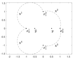
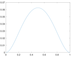
4. Other examples
4.1. NNCC Riemannian manifolds
Let be a compact connected Riemannian manifold, whose geodesic distance is denoted by . Given and define:
-
•
the cut time of by
-
•
the injectivity domain of the exponential map at by
-
•
the cut locus of by
and the cut locus of by .
Proposition 4.1.
Suppose that satisfies
-
•
for each , is a convex subset of ;
-
•
has nonnegative cross-curvature in the sense that for every and every , .
Then satisfies condition (NNCC-conv), and in particular is an NNCC space.
Proof.
Let . By connectedness and completeness of there exist minimizing geodesics joining to respectively and . The tangent vectors at encoding the geodesics are denoted by . Then for any small enough, and belong to .
Since is convex it contains for every , where . Let . Let . Again we may find a minimizing geodesic connecting to whose initial velocity we denote . Then for small enough, and since belongs to there exists a c-segment from to , where .
From the computations by Kim and McCann in [42, Theorem 2.10], we have convexity of the map . Taking the limit , followed by the limit , we obtain convexity of the map , where is defined by . ∎
Note that variational c-segments on Riemannian manifold are not unique in general, as it is already the case for geodesics. There are not many examples of Riemannian manifolds that are nonnegatively cross-curved in the differentiable sense. Kim and McCann [42, Remark 3.4 and Section 6] show the sphere to have nonnegative cross-curvature outside of its cut locus. Then Proposition 4.1 imply:
Corollary 4.2.
Spheres and products of spheres satisfy (NNCC-conv), and are thus NNCC spaces.
In the next section, Proposition 4.5 directly extends this result to (a part of) an infinite dimensional sphere.
4.2. Hellinger distance and Fisher–Rao metric on probability measures
The Hellinger distance on , the set of probability measures on a measurable space , is defined by
| (4.1) |
where is any dominating measure for both measures . This distance is well-known in statistics, popularized by Le Cam for its use for hypothesis testing. The Hellinger distance also appears as a limit case in the unbalanced optimal transport distance (see Section 4.5) but on the cone of nonnegative Radon measures. There it has the geometry of a Hilbert space via the square root transform. In contrast, the geometry of the Hellinger distance on the space of probability measures is rather an infinite dimensional sphere endowed with an ambient metric.
Theorem 4.3.
Let be the unit sphere in a Hilbert space endowed with the ambient squared distance. If satisfies for all and is maximal under the inclusion for this condition, then satisfies (NNCC-conv) and is thus an NNCC space.
Proof.
Consider a triple . The squared ambient Hilbert metric on the sphere reads
| (4.2) |
The equation defining a c-segment at point is
| (4.3) |
where is the orthogonal projection of on . We have information only on the orthogonal part, so the c-segment is not well defined. We propose the following candidate for a variational c-segment:
| (4.4) |
This path satisfies the boundary conditions since by hypothesis and . We now show that the path is contained in . Let . We use the concavity of to ensure that
| (4.5) |
As a consequence,
| (4.6) |
By maximality of the set , we have .
Consider a point , and decompose it into . Note that is less than . Then, we have
| (4.7) | ||||
| (4.8) |
The last term on the r.h.s. is linear. The function is convex as the composition of a convex decreasing function and a concave function . Since , it implies that the quantity in (4.7) is convex in . ∎
Up to taking a square root, the space of probability measures endowed with the squared Hellinger distance of probability measures is a part of the sphere satisfying the maximality condition in Theorem 4.3 so that the NNCC property holds.
Corollary 4.4.
The space satisfies (NNCC-conv) and is thus NNCC.
Proof.
Consider a triple , and their square root densities, with respect to a common dominating measure . Consider the Hilbert space . Then, the set is maximal. One can then apply Theorem 4.3 to obtain the NNCC property on this subset. Denoting the c-segment in the square roots of measures, we get . From this formula, we observe that the c-segment does not depend on the choice of the reference dominating measure, which implies the result. ∎
Note that endowed with the Hellinger distance is not a length space. The associated length space is induced by the metric tensor induced by the Hellinger distance which is called the Fisher–Rao metric tensor. The corresponding geometry on the space of probability measures is an infinite-dimensional sphere with the intrinsic distance. The Fisher–Rao distance reads
| (4.9) |
Since the finite-dimensional sphere is NNCC, one can expect this result to hold in infinite dimensions. Indeed, the space endowed with the Fisher–Rao distance squared is NNCC.
Proposition 4.5.
The space satisfies (NNCC-conv) and is thus NNCC.
Proof.
We construct explicitly the c-segments. Consider a triple and a measure dominating them. Note that since they are nonnegative functions, their mutual distances on the sphere are bounded by . Introduce the square root of their densities with respect to , denoted by . We use the scalar product and consider an orthonormal family for which we can write
| (4.10) | ||||
| (4.11) |
Consider the -dimensional sphere embedded in whose canonical basis is . Recall that the logarithm map on the sphere is defined by where denotes the orthogonal projection on the tangent space on the sphere at point . As a direct consequence of this formula, the c-segment between and lies in the span of . Let us denote such a c-segment by .
It defines a curve in the space of square roots of probability measures also denoted by . Let us compute, for any square-root density , with orthogonal to the span of
| (4.12) |
Since this formula only uses coordinates on the -dimensional sphere, it is convex since the sphere is NNCC. Indeed, it suffices to consider the vector on the -dimensional sphere corresponding to where is the canonical basis of to obtain the same quantity as in (4.12).
Now, we prove that the c-segment defines the square root of a density. We slightly change the notations for simplification. Recall the exponential map at a point on the sphere embedded in the Euclidean space,
| (4.13) |
where is a tangent vector at point . Consider the linear interpolation in this tangent space given by a c-segment as above. An important property of the c-segment above is that since it is a linear interpolation of a vector of length bounded by : indeed, one has . We assume that at the endpoints , it is a nonnegative function. Then, we aim to show that for a linear interpolation of is a nonnegative function for all time . It suffices to show that is a nonnegative function. We have, taking the scalar product with a nonnegative function ,
| (4.14) |
The second term is linear and the first term is concave. Indeed, a direct computation gives that the real function is a decreasing and concave function on so that the composition with is concave. Thus, Formula (4.14) gives a concave function so that it is lower bounded by the minimum value at and which is nonnegative for any admissible test function . This implies the result. ∎
4.3. Relative entropy, a.k.a. the Kullback–Leibler divergence
Given two Borel probability measures on a separable Hilbert space , the relative entropy or Kullback–Leibler divergence between and is defined by
| (4.15) |
with . In (4.15) means that is absolutely continuous with respect to : for every Borel subset of , we have . Since the relative entropy can formally be seen as a Bregman divergence over the space of probability measures , we can expect to have nonnegative cross-curvature. That is indeed the case. To prove it, we use the dual formulation of relative entropy stated in [2, Lemma 9.4.4]
| (4.16) |
where is the space of continuous and bounded functions on endowed with a weaker normed topology, see [2, Section 5.1.2].
Proposition 4.6.
is an NNCC space.
Proof.
Fix such that . Define . Fix . Let us prove the NNCC inequality: for any ,
| (4.17) |
By joint convexity of the relative entropy, we have that .
We now show that if at least one of the two quantities for is infinite, say , then is infinite for : First, if for either does not satisfy , then it is also the case for , which implies that . Second, assume that the measures are absolutely continuous w.r.t. and . Consider the measurable set , then since is increasing for :
| (4.18) |
We obtain, by integration w.r.t.
| (4.19) |
where the last inequality is obtained since for , the entropy function is bounded by a constant . This implies that for . Thus, the inequality (4.17) is trivially satisfied for since both sides are equal to . Last, the case is trivial.
Assume now that both quantities , are finite. Then, is a common dominating measure for all the four measures introduced above. By convexity (w.r.t. the second variable), is finite for all . Using the dual formulation, for with finite relative entropy w.r.t. and , we have
| (4.20) | ||||
| (4.21) |
Since and more precisely , one can write, introducing the measurable function ,
| (4.22) |
and taking the infimum pointwise in gives if and otherwise. Then, taking the supremum in in (4.21) gives
| (4.23) |
Note that the integrability of the negative part of comes from the fact that
| (4.24) |
since is bounded above by . Applying the previous equality to , we obtain
| (4.25) |
The same equality is also valid for . Subtracting the two equalities shows that the inequality (4.17) is an equality. ∎
4.4. Bures–Wasserstein
In this section, we show that the set of Positive Semi-Definite (PSD) real valued matrices endowed with the Bures–Wasserstein squared metric
| (4.26) |
where denotes the unique square root of a PSD matrix , is NNCC. Interestingly, this is an example of Riemannian manifold with boundary, the latter being given by the set of singular PSD matrices . In [5], it is shown that
| (4.27) |
for any , where is the Fröbenius norm and is the orthogonal group of matrices in dimension . In fact, the map is a Riemannian submersion between the linear group of matrices endowed with the Fröbenius norm and the space of positive definite matrices endowed with the Bures–Wasserstein metric. Applying the result by Kim and McCann on Riemannian submersions [42, Theorem 4.5], one can therefore deduce that has nonnegative cross-curvature. However, since is a Riemannian manifold with boundary, the aforementioned theorem cannot be applied on the whole space. We will resort instead to Proposition 2.20.
Theorem 4.7.
The space satifies (NNCC-conv) and is thus an NNCC space.
Remark 4.8.
The space of non-degenerate Gaussian measures forms a geodesically complete subspace in the -Wasserstein space . Since they are parametrized by their mean and covariance matrix, it gives a metric on the space which is precisely given by
| (4.28) |
where is the Euclidean norm. Thanks to Proposition 2.13, the space is NNCC. More generally, the space is NNCC.
Proof.
To apply Proposition 2.20, consider the following surjective map
where is the set of matrices. The space is a Hilbert space and therefore satisfies (NNCC-conv) and is an NNCC space (see Example 2.8). The projected cost on is the Bures–Wasserstein distance squared from (4.27). Since any (where we recall that if ) can be written as for a unitary matrix , this implies
Assumption 2.18 is therefore satisfied, is a cost submersion and satifies (NNCC-conv) (see Remark 2.21). ∎
The previous proof does not provide the form of variational c-segments. This can be useful for applications.
Proposition 4.9.
For , consider the corresponding unique square roots and and the following unitary matrices
where is any right inverse of . Then, curves of the form , with and , are variational c-segments. The curve is unique if the matrices , for , are invertible.
Proof.
To construct variational c-segments from to , we need first to find such that and and are optimal couples. Then, given the variational c-segment in the space , from Lemma 2.19 the curve is a variational c-segment in .
In (4.27), an optimal matrix for is given by any unitary matrix in the polar decomposition of , that is any unitary matrix such that
(see [5, Theorem 1] for details). Then, choosing and for , where
with any right inverse of , we have
Hence, the couples and chosen in this way are optimal. The polar decompositions of are unique if these are invertible, in which case the matrices are uniquely determined.
∎
Remark 4.10.
The family of variational c-segments constructed above is not necessarily exhaustive, as there may exist variational c-segments on the projected space which are not projections of variational c-segments from the above space.
We highlight that for , variational c-segments with respect to the cost correspond to generalized geodesics in the -Wasserstein space . This can be intuitively understood since the space of zero-mean non-degenerate Gaussian measures endowed with the quadratic Wasserstein distance is totally geodesic in the quadratic Wasserstein space on . Consider the three Gaussian measures , and . The optimal transport cost from to and from to is provided by the linear maps , , where
The generalized geodesic from to can be defined in this case simply as , for . The measure is a non-degenerate Gaussian if there exists , , such that
It holds:
where we used that for . The matrix is positive definite since the matrix
is positive definite, as a square of a linear combination of positive definite matrices, and is invertible. The curve coincides with the one provided by Proposition 4.9.
4.5. Unbalanced optimal transport
In this section, we consider the case of the space of nonnegative Radon measures endowed with the unbalanced optimal transport cost. We refer the reader to [74] for an overview. Our main result relies on the conic formulation of unbalanced optimal transport.
4.5.1. Conic formulation of unbalanced optimal transport
We are interested in a natural extension of optimal transport that gives a distance on nonnegative finite Radon measures. Let us start with the particular case of the Wasserstein–Fisher–Rao metric [17], also called Hellinger–Kantorovich [48]. It is usually presented as a relaxed Kantorovich problem, but we prefer to start with the dual formulation. For two positive Radon measures on , with a Polish space,
| (4.29) |
subject to
| (4.30) |
for every . We can derive at least formally -segments. If the supremum is achieved for a potential which is well-defined, we have
| (4.31) |
so that the c-segments correspond to linear interpolation of . Therefore, we get
| (4.32) |
To obtain the -segment , one needs to find if it exists, the corresponding measure for which this potential would be optimal. As characterized in [29], a potential is optimal if it is the c-concave function where is the cost used in the dual formulation constraint (4.30). Similarly to standard optimal transport, if the space of positive Radon measure endowed with the cost has nonnegative cross-curvature, the interpolation defined above gives an optimal potential. Let us generalize this discussion to more general entropy-transport problems in the spirit of [48]. In this section, we work on a closed manifold to simplify the presentation and avoid non-compactness issues.
Definition 4.11.
An entropy function is a convex, lower semi-continuous, nonnegative function such that and if . Its recession constant is defined as .
Definition 4.12.
Let be an entropy function and be Radon measures on , a Polish space. The Csiszàr divergence associated with is
where is the orthogonal part of the Lebesgue decomposition of with respect to .
For , is the Kullback–Leibler divergence or relative entropy, and it reads
| (4.33) |
Definition 4.13 (Entropy-Transport problem).
Let and be entropy functions. The unbalanced optimal transport problem is defined as
| (4.34) |
where are marginals of , and is a cost function which is bounded below and continuous at each point where it has finite value.
We underline the fact that the cost may be unbounded and it is the case for the Wasserstein–Fisher–Rao metric for which and the entropy functionals are the Kullback–Leibler entropy. This problem has an equivalent definition on the cone over the base space denoted by . The product of cones is endowed with the following cost ,
| (4.35) |
This cost is obtained by taking an infimum on the perspective function of the function . As a consequence of the perspective function, it is one-homogeneous in and convex in . One of the main results in [48] is the equivalence between Definition 4.13 and an optimal transport problem with moment constraints instead of marginal constraints:
Definition 4.14 (Conic formulation).
Let be two positive Radon measures. Define
| (4.36) |
where denotes the set of positive Radon measures on such that
| (4.37) |
where are the two respective projections on .
It is proven in [48] that . To give more insight, hereafter are a few important instances of conic and static formulations.
Example 4.15.
Choose the Kullback–Leibler divergence or relative entropy. Then, there are two important cases:
-
•
The WFR case with . The cost on the cone is
(4.38) Note that the parametrization chosen here differs from the usual Riemannian cone which uses the following formula, for a distance on the base space
(4.39) There is no difference up to a square root change of variable in the radial variable.
-
•
The Gaussian-Hellinger case with , .
A last example is the partial optimal transport case for which and with . One has .
4.5.2. Main result
We now prove a simple lemma, reminiscent of the lemma proven in [48, Lemma 7.11]. This lemma uses the homogeneity of the cost and the fact that the constraints on the marginals are moment constraints, which are invariant to rescaling: namely, and have the same moment with respect to as defined in Eq. (4.37).
Lemma 4.16.
Let and non null, be positive Radon measures and such that . Then, there exists such that
| (4.40) |
Theorem 4.17.
The space of positive Radon measures endowed with the cost in Definition 4.14 (equivalently ) for the cost on is NNCC if is NNCC.
Example 4.18.
The simplest example is the -dimensional sphere for which the Riemannian cone (see Formula (4.39)) is the Euclidean space endowed with the Euclidean squared distance which has the NNCC property. Therefore, the space of nonnegative measures on the sphere endowed with the Wasserstein–Fisher–Rao metric has the NNCC property.
Example 4.19 (Optimal transport on the cone of positive symmetric matrices).
Another important example is related to the Bures–Wasserstein metric. Indeed, the space of positive definite matrices is itself a cone: Let us parameterize a (non zero) nonnegative matrix by with the space of unit trace symmetric (positive semi-definite) matrix. Associated with the Bures metric, the Bures angle or quantum angle is defined between two unit trace matrices :
| (4.41) |
Using Formula (4.38) and by definition, the cone over endowed with the Bures length gives the Bures metric. In particular, the cone over the space of positive matrices of unit trace endowed with the usual Bures metric gives the Bures–Wasserstein metric: . Since has the NNCC property (see Theorem 4.7), Theorem 4.17 applies: the unbalanced optimal transport metric on has the NNCC property.
A direct consequence of the cost submersion fact is that lifted c-segments in UOT are projections of lifted c-segments on the probability measures on the cone. Let us conclude this section with a remark on the necessity of the cone to be NNCC for the NNCC property of UOT. In the Wasserstein–Fisher–Rao case, we conjecture an equivalence between the two properties when the diameter of the underlying manifold is less than since, in such a case, the geometry of the cone is completely encoded in the geometry of unbalanced optimal transport via Dirac masses.
4.6. Gromov–Wasserstein
In this section we show that the set of all metric measure spaces, or more generally gauged spaces, equipped with the squared Gromov–Wasserstein distance is an NNCC space. This represents a significant advance over Sturm’s discovery [73] that the “space of spaces” is positively curved, see Remark 4.23.
A metric measure space is a triple , where is a complete separable metric space and is a Borel probability measure on . The Gromov–Wasserstein distance, as introduced by Mémoli [60] and also studied by Sturm [73], is a way to compare two metric measure spaces in terms of their intrinsic qualities, up to isometries. In particular one considers equivalence classes defined as follows: two metric measure spaces and are equivalent if there exists a map which is an isometry on the support of and such that . The set of all equivalence classes of metric measure spaces will be denoted by .
The Gromov–Wasserstein distance between and is defined by
| (4.42) |
This is a metric on valued in . From an optimization viewpoint, problem (4.42) is harder than optimal transport since it is a nonconvex quadratic optimization problem. However, as shown in [73, Theorem 3.1], the structure of geodesics is rather simple. Once an optimal plan is found between and , the geodesic consists of , which suggests there may also be a particularly simple form of variational c-segments. This is indeed the case:
Proposition 4.20 (Variational c-segments for Gromov–Wasserstein).
Let , , be such that and let be an optimal plan for (). Consider any -plan such that and , and define for every
| (4.43) |
and , . In the expression of , acts on the components and on the components of . Then is a variational c-segment on .
Theorem 4.21.
is an NNCC space.
Proof of Proposition 4.20.
Let , , , denote four (equivalence classes of) metric measure spaces. For , let be an optimal Gromov–Wasserstein coupling of . Then
| (4.44) |
Define by (4.43) and fix . Since is a coupling of we have the inequality
| (4.45) |
Let , which we will optimize over in a moment to obtain the term . Assume without loss of generality that
for if the above value is infinite then the desired conclusion (4.47) holds automatically. Glue and along into a -plan . Using (4.45) we may write
| (4.46) |
where depends on , on and on . By expanding the square, we see that is an affine function of . Therefore the right-hand side of (4.46) is affine in and we can write
| (4.47) |
We recognize (4.44) for in the right-hand side. Finally taking a supremum over we obtain the NNCC inequality
Note in particular that choosing implies finiteness of . ∎
Remark 4.22.
In the proof of Proposition 4.20, the fact that are distances is not used. Therefore the result holds for more general functions, such as gauge functions [73, Section 5].
Remark 4.23 (NNCC and PC).
Consider the subspace of metric measure spaces with finite size . Sturm proved that is a geodesic space that is positively curved in the sense of Alexandrov [73, Theorem 4.4]. The proof of Proposition 4.20 shows just as well to be an NNCC space, a stronger property than positive curvature by Proposition 2.26.
4.7. Procrustes–Wasserstein
In a similar spirit to Gromov–Wasserstein distances, comparing probability measures in the Euclidean space up to isometries has been addressed in the applied mathematics literature: one candidate is the Procrustes–Wasserstein distance, which is defined by
| (4.48) |
where are isometries of and are two probability measures on . Sometimes, it is also defined as the quotient with the group of rotations only after the alignment of the mean of the two measures, see [34].
Theorem 4.24.
The space endowed with the cost is NNCC.
Proof.
Since is NNCC, Proposition 2.20 on cost submersions shall imply the theorem. We now check that the hypotheses of Proposition 2.20 are fulfilled. Note that by a change of variables, one has . Under the additional fact that the infimum of the minimization problem is attained in , then the formula (2.18) follows directly. To prove the existence of minimizers, we prove that one can restrict the optimization to a compact subset of isometries. Note that is a semidirect product of groups between translations and rotations. It is sufficient to reduce the set of translations to a compact set. For that, we note that by the convexity of the Euclidean distance squared . As an immediate consequence, the norm of the translation part of is bounded by . ∎
Remark 4.25.
Note that the result is obvious when one considers the quotient only with instead of due to the compactness of . In the same direction, this result directly extends to Riemannian manifolds that satisfy the two conditions:
-
(i)
is NNCC where is the Riemannian distance.
-
(ii)
The isometry group of is compact.
Indeed, in such a case, it satisfies the hypotheses of a cost submersion in Definition 2.17 and one can apply Proposition 2.20.
Appendix A Infinite values
In this appendix, we show how to manipulate infinite values taken by the cost function and by potentials. Here are our main references. Moreau [62, Section 4.c.] considers costs taking both values and explains how to deal with undefined expressions of infinites. He has opposite signs in regard to potentials. Villani [83, Chapter 5] is a main reference, he only considers costs taking the value. Rockafellar and Wets [68, Chapter 1] define epigraphs and hypographs of extended-real-valued functions in standard convex analysis.
Hypographs
Since here we want to work with c-concave functions we consider hypographs. Given an arbitrary set and a function , the hypograph of is the subset of defined by
| (A.1) |
Note that is always finite, thus is a subset of the product of with the real numbers, and not with the extended real numbers. In particular given , if then then the intersection of and the vertical line is empty, and if then contains the vertical line . If is finite then the intersection of and is and we call the “fiber above ”. The domain of is the set of ’s such that the vertical line intersects the hypograph of , i.e. .
Let denote the class of all subsets that satisfy the property:
-
For every , the fiber above is either empty or a closed interval of unbounded to the left (this includes itself).
Clearly if is the hypograph of a function then it belongs to . Then realizes a one-to-one correspondence between functions and . Given , we may find the corresponding function by
| (A.2) |
with , and the convention .
A simple but important property of the class of hypographs is that it is closed under arbitrary intersections. Indeed we can reason fiber by fiber and then use the fact that a class of intervals of that are closed and unbounded to the left is closed under arbitrary intersections.
Let us now consider a cost function , where is another arbitrary set. To fix ideas, we will deal with functions and that satisfy the sign .
c-transform
The c-conjugate of an arbitrary subset is the subset defined by
If is empty then by convention. We see that for any , . More precisely and in view of (A.2), is the hypograph of the function defined by
| (A.3) | ||||
| (A.4) |
When for some , we define by and call the c-transform of . We see that
| (A.5) | ||||
where in the last infimum the following rule should be used: and . It may be convenient to remember that the rule for undefined expressions and is to give the neutral element for , i.e. . By exchanging the roles of and we similarly define c-conjugates of subsets and c-transforms of functions , still denoted by and by respectively.
We say that a function is c-concave if there exists such that . This is equivalent to the existence of a function such that , or to . We may similarly define c-concave functions on .
Contact set
We say that two subsets and are sub-conjugate if for every . This can be written as
| (A.6) |
which shows sub-conjugation to be a symmetric relation for and . Sub-conjugation is called sur-dualité by Moreau who has opposite signs [62]. Given two sub-conjugate subsets and and , their contact set is defined by
| (A.7) |
and by (A.6) the inequality is in fact an equality. Therefore the quantity in (A.7) is finite.
We say that two functions and are sub-conjugate if the sets and are sub-conjugate. We see that this can be written as
with the rule in the left-hand side, or in other words whenever the left-hand side is well-defined. By (A.5) this is also equivalent to and . In particular and are always sub-conjugate. The contact set of and is called the c-subdifferential of , and can be encoded as only those pairs that satisfy , since combining (A.6) and (A.7) forces and (and in turn these are finite). More generally since a sub-conjugate pair satisfies we may ask for . In short, the c-subdifferential of an arbitrary function can be defined as
| (A.8) |
We can then set for any ,
| (A.9) |
We could similarly define the c-subdifferential of a function defined on .
Appendix B Proofs
B.1. Proof of Theorem 2.16
In this section we prove our extension of the Riemannian submersion result of Kim and McCann to the case of a principal fiber bundle endowed with a cost diagonally invariant to a group action. Let us recall first Definitions 2.14 and 2.15.
Definition B.1 (Submersion and projection of a cost.).
Let for be two submersions between manifolds with compact fibers and be a continuous cost. Define the projected cost by
| (B.1) |
Definition B.2 (Principal bundle with -invariant cost).
Consider a principal fiber bundle where is a compact Lie group and a continuous cost such that leaves the cost invariant. Namely, we assume
| (B.2) |
We consider the projection . The corresponding projected cost is denoted .
Under the assumptions of Definition B.2, let and . Then, we can define the set of optimal lifts of at point by . Similarly, we can define the set of optimal lifts . If this minimization leads to a unique point, this enables the definition of lift of curves by . The fact that the optimal lifts exist to any given is because the action of on the product leaves the cost invariant so that one can fix the pre-image of : .
We make the following assumption:
Assumption B.3.
The lifting procedure is well-defined for curves, meaning that locally, there is a unique point at which the infimum cost is attained and that it is a smooth operation.
In particular, if the curve is for then the curve is also . This is satisfied for instance in the case of Riemannian submersions which have the structure of a principal fiber bundle. Assuming that the lift of curves is well-defined implies that the lift of tangent vectors is also well-defined. We call it horizontal lift, similar to the Riemannian submersion case. The most important fact in this construction is that the lifts of c-segments are c-segments and this fact relies crucially on the invariance of the cost:
Proposition B.4 (Lift of c-segments).
Under Assumption B.3, the lift of a c-segment on is a c-segment on .
Proof.
The definition of a c-segment on reads
| (B.3) |
Consider the lift of the c-segment denoted by . Due to the invariance of the cost on , we have . Now, due to the optimality of the lift, the first-order optimality condition gives
| (B.4) |
for all and . Note that the notation is defined as the tangent vector at given by the differentiation of a curve starting at identity with initial tangent vector . The previous formula means that the differentiation of the cost in the vertical direction (the tangent space to the fiber) vanishes. By local trivialization of the fiber bundle, equations (B.3) and (B.4) imply that is a c-segment on . ∎
This fact allows us to prove Theorem 2.16.
Proof of Theorem 2.16.
The proof follows the one of [42, Theorem 4.5] and we include it here to ease the reader. Consider the lift at point of the c-segment in a neighborhood of . Consider also a curve also defined on a neighborhood of , with tangent vector at and the lift of at the point . One can now consider the function which is nonnegative by definition of . We now use the definition of the cross-curvature
| (B.5) |
so that in order to prove the result it is sufficient to prove that . In addition to nonnegativity, by its definition which implies that achieves its minimum on these two sets and the Hessian of is a positive semi-definite matrix. This Hessian must vanish since the diagonal terms are by differentiation of and it implies by nonnegativity of the Hessian matrix . It implies that the Taylor expansion of takes the form
| (B.6) |
with similar notations to [42, Proof of Theorem 4.5], where the authors proved that by differentiation of and . The Taylor expansion of is reduced to so that nonnegativity of directly implies which is the result. ∎
Remark B.5.
The result of the theorem is local. As a consequence, Assumption B.3 can be replaced with a local version, i.e. the optimal lifts are well-defined in a neighborhood of .
B.2. Proof of Theorem 3.10
Condition (NNCC-conv) is a stronger property with respect to NNCC as it requires the function to be convex along variational c-segments , for any . That is, the NNCC inequality must be satisfied for any subinterval : The restriction of a variational c-segment from to should remain a variational c-segment between and . In order to lift condition (NNCC-conv) to the Wasserstein space, we need to refine the definition of lift. We make the following assumption:
Assumption B.6.
(NNCC-conv)-variational c-segments on are continuous curves on with limits at and .
We denote by the space of curves valued in that are continuous on with limit at and .
Definition B.7 ((NNCC-conv)-lifted c-segments).
Let be a path in and let . We say that is an (NNCC-conv)-lifted c-segment from if there exist a measurable set a collection of measurable maps (), and a -plan such that
-
(i)
is concentrated on , i.e. , and and ;
-
(ii)
, , and is an (NNCC-conv) variational c-segment on for each ;
-
(iii)
and are respective optimal couplings of and for the cost ;
-
(iv)
there exists such that , where is the evaluation at time .
The set is defined as in (3.3). Note that since the cost function is now continuous, it is in particular real valued and coincides with . With respect to Definition 3.1, we require now the additional condition that the collection of measurable maps have a specific form, composition of the evaluation at time and a measurable map mapping from to the set of curves . Assumption B.6 ensures that the collection of measurable maps exists.
Lemma B.8 (Existence of (NNCC-conv)-lifted c-segments).
Let satisfies condition (NNCC-conv), for and Polish spaces and a continuous cost function bounded from below, satisfying further Assumption B.6. Then for any and such that and , there exists a (NNCC-conv)-lifted c-segment from between and .
Proof.
Compared to Lemma 3.3, we need now to guarantee the existence of a measurable selection as a map from to the set of curves valued in that are continuous on with limit at and .
The (NNCC-conv) property guarantees the existence of an (NNCC-conv)-variational c-segment for each triplet . We aim to construct a measurable map mapping each triplet to the evaluation at time of an associated (NNCC-conv)-variational c-segment. Consider then the multi-valued map which maps a given triplet to the set of (NNCC-conv)-variational c-segments associated with it. By the assumptions, the graph of is the set
where is endowed with the uniform norm topology. Note that this is a Suslin space (see [8]) since it is isomorphic to . By [8, Theorem 6.9.13], it is sufficient to show that the graph of is closed to guarantee the existence of a measurable selection as in Definition B.7. This is true since the convex constraint in 1 can be formulated as an intersection of closed subsets due to the continuity of the cost. Again by continuity of the curves on , the evaluation is continuous for and therefore the map is measurable. ∎
Proof of Theorem 3.10.
Thanks to the new definition of lift, for any triplet , the following inequality holds for any
Moreover, as pointed out in Remark 3.8, the transport plan as defined in the proof of Proposition 3.5 is optimal for any . These two facts combined ensure that one can repeat the proof of Proposition 3.5 on any subinterval , implying that the restriction of a lifted c-segment to is again a variational c-segment in . (NNCC-conv)-lifted c-segments satisfy therefore condition (NNCC-conv). The claim of Theorem 3.10 is a direct consequence. ∎
B.3. Other proofs
Proof of Lemma 2.33.
Using a similar argument as in the proof of Lemma 2.5, we obtain
| (B.7) |
for all . This inequality implies that for some real coefficients . Indeed, one can test this inequality with orthogonal to the span of the two vectors. The inequality reduces to a two-dimensional problem. The first case is when , then any candidate satisfies our statement, in particular .
The second case is when the two vectors on the right-hand side of (B.7) span a two-dimensional space. Testing the inequality with a vector such that , we get and testing with the opposite, we get . A similar reasoning gives that . Now, we consider to obtain that is contained in the segment. The result is then implied by the continuity of the curve since the coefficient is unique. The last case when and are colinear but different is similar. ∎
Proof of Lemma 3.2.
Let be defined as in (3.3). The NNCC property guarantees the existence of a variational c-segment for each triplet . For each we aim to construct a measurable map mapping -a.e. triplet to the evaluation at time of an associated variational c-segment.
Fix and consider the multi-valued map which maps a given triplet to the (nonempty by hypothesis) set of points that satisfy the NNCC inequality (2.11). By [8, Theorem 6.9.13], it is sufficient that the graph of is measurable to prove the existence of a measurable selection . Consider the two transport plans defined as , for . Since is lower semi-continuous and bounded from below (and taking finite values on ), it can be approximated by a non-decreasing sequence of continuous costs, denoted , . By Egorov’s theorem and the fact that is Polish, this pointwise convergence can be turned into a uniform convergence on a compact set , for and two compact sets of measure and , for every integer (see [83, Proof of Theorem 5.10]). For every , there exists such that for , we have
| (B.8) |
For integer, consider the inequality
| (B.9) |
Define the closed sets (since is continuous)
| (B.10) |
By (B.8) and the triangle inequality, defining
we have and , a.e. Finally, by pointwise convergence, , a.e. Then, there exists a measurable set such that and we can change on by choosing the value , for instance (in fact any measurable extension would work). Denoting
we have the union . Being a countable union and intersection of measurable sets, is itself measurable. Then, the selection theorem can be applied and it gives the result. ∎
Remark B.9.
The previous proof is inspired from [83, Proof of Theorem 5.10] in which a similar measurability issue is treated.
Proof of Lemma 4.16.
We first use [48, Lemma 7.12] which says that given marginals , there exist lifts realizing Equation (4.40) (replacing by ). However, the measure is not necessarily equal to which is fixed in our setting. In fact, [48, Lemma 7.12] shows that it is possible to fix the marginal to , which we use in the rest of the proof. Denote an optimal plan on the cone between the measures and . This optimal plan only charges due to the marginal constraint , so that when is fixed, it defines a measure on by disintegration:
| (B.11) |
We consider the plan defined by its disintegration with respect to
| (B.12) |
where for , which is a map on . By definition, the marginal of on is . We consider a function that is one-homogeneous with respect to the couple of radial variables . One has
| (B.13) | ||||
| (B.14) | ||||
| (B.15) | ||||
| (B.16) |
It implies that the cost of the plan is preserved since the cost on the product of cones is one-homogeneous. Moreover, the marginal constraint on can be tested by functions of the type where which is also homogeneous with respect to . ∎
Acknowledgements
We wish to thank T. Gallouët, Y.-H. Kim, H. Lavenant, and G. Loeper for helpful discussions. FXV and GT would like to thank the Mathematisches Forschungsinstitut Oberwolfach for hosting in 2024 the workshop 2406, during which this work has advanced significantly. The work of FXV and GT is supported by the Bézout Labex (New Monge Problems), funded by ANR, reference ANR-10-LABX-58.
References
- [1] A. D. Aleksandrov, A theorem on triangles in a metric space and some of its applications, Trudy Matematicheskogo Instituta imeni VA Steklova, 38 (1951), pp. 5–23.
- [2] L. Ambrosio, N. Gigli, and G. Savaré, Gradient flows in metric spaces and in the space of probability measures, Lectures in Mathematics ETH Zürich, Birkhäuser Verlag, Basel, second ed., 2008.
- [3] S. Barberà, An introduction to strategy-proof social choice functions, Soc. Choice Welf., 18 (2001), pp. 619–653.
- [4] V. N. Berestovskiĭ, “Submetries” of three-dimensional forms of nonnegative curvature, Sibirsk. Mat. Zh., 28 (1987), pp. 44–56, 224.
- [5] R. Bhatia, T. Jain, and Y. Lim, On the Bures–Wasserstein distance between positive definite matrices, Expo. Math., 37 (2019), pp. 165–191.
- [6] M. Bichler, Market design: a linear programming approach to auctions and matching, Cambridge University Press, 2017.
- [7] S. G. Bobkov and M. Ledoux, From Brunn–Minkowski to Brascamp–Lieb and to logarithmic Sobolev inequalities, Geom. Funct. Anal., 10 (2000), pp. 1028–1052.
- [8] V. I. Bogachev, Measure theory. Vol. I, II, Springer-Verlag, Berlin, 2007.
- [9] C. Bonet, B. Malézieux, A. Rakotomamonjy, L. Drumetz, T. Moreau, M. Kowalski, and N. Courty, Sliced-Wasserstein on symmetric positive definite matrices for M/EEG signals, in Proceedings of the 40th International Conference on Machine Learning, vol. 202 of Proceedings of Machine Learning Research, PMLR, 23–29 Jul 2023, pp. 2777–2805.
- [10] T. Börgers, An introduction to the theory of mechanism design, Oxford University Press, USA, 2015.
- [11] D. Burago, Y. Burago, and S. Ivanov, A course in metric geometry, vol. 33 of Graduate Studies in Mathematics, American Mathematical Society, Providence, RI, 2001.
- [12] Y. Burago, M. Gromov, and G. Perel’man, A. D. Aleksandrov spaces with curvatures bounded below, Uspekhi Mat. Nauk, 47 (1992), pp. 3–51, 222.
- [13] L. A. Caffarelli, The regularity of mappings with a convex potential, J. Amer. Math. Soc., 5 (1992), pp. 99–104.
- [14] , Boundary regularity of maps with convex potentials. II, Ann. of Math. (2), 144 (1996), pp. 453–496.
- [15] G. Carlier, A general existence result for the principal-agent problem with adverse selection, J. Math. Econom., 35 (2001), pp. 129–150.
- [16] Y. Chen, T. T. Georgiou, and A. Tannenbaum, Optimal transport for gaussian mixture models, IEEE Access, 7 (2019), pp. 6269–6278.
- [17] L. Chizat, G. Peyre, B. Schmitzer, and F.-X. Vialard, Unbalanced optimal transport: dynamic and Kantorovich formulations, J. Funct. Anal., 274 (2018), pp. 3090–3123.
- [18] D. Cordero-Erausquin, R. J. McCann, and M. Schmuckenschläger, A Riemannian interpolation inequality à la Borell, Brascamp and Lieb, Invent. Math., 146 (2001), pp. 219–257.
- [19] , Prékopa-Leindler type inequalities on Riemannian manifolds, Jacobi fields, and optimal transport, Ann. Fac. Sci. Toulouse Math. (6), 15 (2006), pp. 613–635.
- [20] M. Cullen and H. Maroofi, The fully compressible semi-geostrophic system from meteorology, Arch. Ration. Mech. Anal., 167 (2003), pp. 309–336.
- [21] P. Delanoë, Classical solvability in dimension two of the second boundary-value problem associated with the Monge-Ampère operator, Ann. Inst. H. Poincaré C Anal. Non Linéaire, 8 (1991), pp. 443–457.
- [22] J. Delon and A. Desolneux, A wasserstein-type distance in the space of gaussian mixture models, 2020.
- [23] I. Ekeland and R. Temam, Convex Analysis and Variational Problems, Classics in Applied Mathematics, Society for Industrial and Applied Mathematics, 1999.
- [24] A. Figalli, Y.-H. Kim, and R. J. McCann, When is multidimensional screening a convex program?, J. Econom. Theory, 146 (2011), pp. 454–478.
- [25] A. Figalli and L. Rifford, Continuity of optimal transport maps and convexity of injectivity domains on small deformations of , Comm. Pure Appl. Math., 62 (2009), pp. 1670–1706.
- [26] A. Figalli, L. Rifford, and C. Villani, Nearly round spheres look convex, Amer. J. Math., 134 (2012), pp. 109–139.
- [27] A. Figalli and C. Villani, An approximation lemma about the cut locus, with applications in optimal transport theory, Methods Appl. Anal., 15 (2008), pp. 149–154.
- [28] A. Gallouët, Q. Mérigot, and B. Thibert, Strong c-concavity and stability in optimal transport, arXiv preprint arXiv:2207.11042, (2022).
- [29] T. Gallouët, R. Ghezzi, and F.-X. Vialard, Regularity theory and geometry of unbalanced optimal transport. Dec. 2021.
- [30] W. Gangbo and R. J. McCann, Shape recognition via Wasserstein distance, Quart. Appl. Math., 58 (2000), pp. 705–737.
- [31] R. J. Gardner, The Brunn-Minkowski inequality, Bull. Amer. Math. Soc. (N.S.), 39 (2002), pp. 355–405.
- [32] A. Gibbard, Manipulation of voting schemes: a general result, Econometrica, 41 (1973), pp. 587–601.
- [33] T. Glimm and V. Oliker, Optical design of single reflector systems and the Monge-Kantorovich mass transfer problem, vol. 117, 2003, pp. 4096–4108. Nonlinear problems and function theory.
- [34] E. Grave, A. Joulin, and Q. Berthet, Unsupervised alignment of embeddings with Wasserstein Procrustes, in Proceedings of the Twenty-Second International Conference on Artificial Intelligence and Statistics, vol. 89 of Proceedings of Machine Learning Research, PMLR, 16–18 Apr 2019, pp. 1880–1890.
- [35] N. Guillen and J. Kitagawa, On the local geometry of maps with -convex potentials, Calc. Var. Partial Differential Equations, 52 (2015), pp. 345–387.
- [36] M. Jacobs, W. Lee, and F. Léger, The back-and-forth method for Wasserstein gradient flows, ESAIM Control Optim. Calc. Var., 27 (2021), pp. Paper No. 28, 35.
- [37] M. Jacobs and F. Léger, A fast approach to optimal transport: the back-and-forth method, Numer. Math., 146 (2020), pp. 513–544.
- [38] C. Ju and C. Guan, Deep optimal transport for domain adaptation on SPD manifolds. 2023.
- [39] V. Kapovitch and A. Lytchak, The structure of submetries, Geom. Topol., 26 (2022), pp. 2649–2711.
- [40] Y.-H. Kim, Counterexamples to continuity of optimal transport maps on positively curved Riemannian manifolds, International Mathematics Research Notices, 2008 (2008), p. rnn120.
- [41] Y.-H. Kim and R. J. McCann, Continuity, curvature, and the general covariance of optimal transportation, J. Eur. Math. Soc. (JEMS), 12 (2010), pp. 1009–1040.
- [42] , Towards the smoothness of optimal maps on Riemannian submersions and Riemannian products (of round spheres in particular), J. Reine Angew. Math., 664 (2012), pp. 1–27.
- [43] J.-J. Laffont and D. Martimort, The Theory of Incentives, Princeton University Press, Princeton, 2002.
- [44] P. W. Y. Lee and J. Li, New examples satisfying Ma–Trudinger–Wang conditions, SIAM Journal on Mathematical Analysis, 44 (2012), pp. 61–73.
- [45] P. W. Y. Lee and R. J. McCann, The Ma–Trudinger–Wang curvature for natural mechanical actions, Calc. Var. Partial Differential Equations, 41 (2011), pp. 285–299.
- [46] F. Léger and F.-X. Vialard, A geometric Laplace method, Pure Appl. Anal., 5 (2023), pp. 1041–1080.
- [47] L. Leindler, On a certain converse of Hölder’s inequality. II, Acta Sci. Math. (Szeged), 33 (1972), pp. 217–223.
- [48] M. Liero, A. Mielke, and G. Savaré, Optimal entropy-transport problems and a new Hellinger-Kantorovich distance between positive measures, Invent. Math., 211 (2018), pp. 969–1117.
- [49] G. Loeper, On the regularity of solutions of optimal transportation problems, Acta Math., 202 (2009), pp. 241–283.
- [50] , Regularity of optimal maps on the sphere: the quadratic cost and the reflector antenna, Arch. Ration. Mech. Anal., 199 (2011), pp. 269–289.
- [51] G. Loeper and N. S. Trudinger, Weak formulation of the MTW condition and convexity properties of potentials, Methods Appl. Anal., 28 (2021), pp. 53–60.
- [52] G. Loeper and C. Villani, Regularity of optimal transport in curved geometry: the nonfocal case, Duke Math. J., 151 (2010), pp. 431–485.
- [53] J. Lott and C. Villani, Ricci curvature for metric-measure spaces via optimal transport, Ann. of Math. (2), 169 (2009), pp. 903–991.
- [54] F. Léger and P.-C. Aubin-Frankowski, Gradient descent with a general cost, 2023.
- [55] X.-N. Ma, N. S. Trudinger, and X.-J. Wang, Regularity of potential functions of the optimal transportation problem, Arch. Ration. Mech. Anal., 177 (2005), pp. 151–183.
- [56] D. Matthes and S. Plazotta, A variational formulation of the BDF2 method for metric gradient flows, ESAIM Math. Model. Numer. Anal., 53 (2019), pp. 145–172.
- [57] B. Maurey, Some deviation inequalities, Geom. Funct. Anal., 1 (1991), pp. 188–197.
- [58] R. J. McCann, A convexity theory for interacting gases and equilibrium crystals, ProQuest LLC, Ann Arbor, MI, 1994. Thesis (Ph.D.)–Princeton University.
- [59] R. J. McCann, A glimpse into the differential topology and geometry of optimal transport, Discrete Contin. Dyn. Syst., 34 (2014), pp. 1605–1621.
- [60] F. Mémoli, Gromov–Wasserstein distances and the metric approach to object matching, Found. Comput. Math., 11 (2011), pp. 417–487.
- [61] J. A. Mirrlees, An exploration in the theory of optimum income taxation, The review of economic studies, 38 (1971), pp. 175–208.
- [62] J.-J. Moreau, Inf-convolution, sous-additivité, convexité des fonctions numériques, J. Math. Pures Appl. (9), 49 (1970), pp. 109–154.
- [63] A. Prékopa, Logarithmic concave measures with application to stochastic programming, Acta Sci. Math. (Szeged), 32 (1971), pp. 301–316.
- [64] , On logarithmic concave measures and functions, Acta Sci. Math. (Szeged), 34 (1973), pp. 335–343.
- [65] M. Quinzii and J.-C. Rochet, Multidimensional signalling, J. Math. Econom., 14 (1985), pp. 261–284.
- [66] C. Rankin, A remark on the geometric interpretation of the A3w condition from optimal transport, Bull. Aust. Math. Soc., 108 (2023), pp. 162–165.
- [67] R. T. Rockafellar, Convex analysis, vol. No. 28 of Princeton Mathematical Series, Princeton University Press, Princeton, NJ, 1970.
- [68] R. T. Rockafellar and R. J.-B. Wets, Variational analysis, vol. 317 of Grundlehren der mathematischen Wissenschaften [Fundamental Principles of Mathematical Sciences], Springer-Verlag, Berlin, 1998.
- [69] F. Santambrogio, Optimal transport for applied mathematicians, vol. 87 of Progress in Nonlinear Differential Equations and their Applications, Birkhäuser/Springer, Cham, 2015. Calculus of variations, PDEs, and modeling.
- [70] M. A. Satterthwaite, Strategy-proofness and Arrow’s conditions: Existence and correspondence theorems for voting procedures and social welfare functions, J. Econom. Theory, 10 (1975), pp. 187–217.
- [71] K.-T. Sturm, On the geometry of metric measure spaces, Acta Mathematica, 196 (2006), pp. 65 – 131.
- [72] , On the geometry of metric measure spaces. II, Acta Mathematica, 196 (2006), pp. 133–177.
- [73] , The space of spaces: curvature bounds and gradient flows on the space of metric measure spaces, Mem. Amer. Math. Soc., 290 (2023), pp. v+111.
- [74] T. Séjourné, G. Peyré, and F.-X. Vialard, Chapter 12 - unbalanced optimal transport, from theory to numerics, in Numerical Control: Part B, E. Trélat and E. Zuazua, eds., vol. 24 of Handbook of Numerical Analysis, Elsevier, 2023, pp. 407–471.
- [75] R. Tibshirani, Regression shrinkage and selection via the lasso, Journal of the Royal Statistical Society (Series B), 58 (1996), pp. 267–288.
- [76] N. S. Trudinger and X.-J. Wang, On strict convexity and continuous differentiability of potential functions in optimal transportation, Arch. Ration. Mech. Anal., 192 (2009), pp. 403–418.
- [77] , On the second boundary value problem for Monge-Ampère type equations and optimal transportation, Ann. Sc. Norm. Super. Pisa Cl. Sci. (5), 8 (2009), pp. 143–174.
- [78] J. Urbas, On the second boundary value problem for equations of Monge-Ampère type, J. Reine Angew. Math., 487 (1997), pp. 115–124.
- [79] A. Vacher, B. Muzellec, F. Bach, F.-X. Vialard, and A. Rudi, Optimal estimation of smooth transport maps with kernel sos, SIAM Journal on Mathematics of Data Science, 6 (2024), pp. 311–342.
- [80] A. Vacher, B. Muzellec, A. Rudi, F. Bach, and F.-X. Vialard, A dimension-free computational upper-bound for smooth optimal transport estimation, in Conference on Learning Theory, PMLR, 2021, pp. 4143–4173.
- [81] C. Villani, Topics in Optimal Transportation, Graduate studies in mathematics, American Mathematical Society, 2003.
- [82] , Stability of a 4th-order curvature condition arising in optimal transport theory, J. Funct. Anal., 255 (2008), pp. 2683–2708.
- [83] , Optimal transport, vol. 338 of Grundlehren der mathematischen Wissenschaften [Fundamental Principles of Mathematical Sciences], Springer-Verlag, Berlin, 2009. Old and new.
- [84] R. V. Vohra, Mechanism design, vol. 47 of Econometric Society Monographs, Cambridge University Press, Cambridge, 2011. A linear programming approach.
- [85] X.-J. Wang, On the design of a reflector antenna. II, Calc. Var. Partial Differential Equations, 20 (2004), pp. 329–341.
- [86] O. Yair, F. Dietrich, R. Talmon, and I. G. Kevrekidis, Domain adaptation with optimal transport on the manifold of SPD matrices, 2020.