DiffSSC: Semantic LiDAR Scan Completion using Denoising Diffusion Probabilistic Models

Abstract

Perception systems play a crucial role in autonomous driving, incorporating multiple sensors and corresponding computer vision algorithms. 3D LiDAR sensors are widely used to capture sparse point clouds of the vehicle’s surroundings. However, such systems struggle to perceive occluded areas and gaps in the scene due to the sparsity of these point clouds and their lack of semantics. To address these challenges, Semantic Scene Completion (SSC) jointly predicts unobserved geometry and semantics in the scene given raw LiDAR measurements, aiming for a more complete scene representation. Building on promising results of diffusion models in image generation and super-resolution tasks, we propose their extension to SSC by implementing the noising and denoising diffusion processes in the point and semantic spaces individually. To control the generation, we employ semantic LiDAR point clouds as conditional input and design local and global regularization losses to stabilize the denoising process. We evaluate our approach on autonomous driving datasets and our approach outperforms the state-of-the-art for SSC.

I Introduction

Perception systems collect low-level attributes of the surrounding environment, such as depth, temperature, and color, through various sensor technologies. These systems leverage machine learning algorithms to achieve high-level understanding, such as object detection and semantic segmentation. 3D LiDAR is widely used in self-driving cars to collect 3D point clouds. However, 3D LiDAR has inherent limitations, such as unobservable occluded regions, gaps between sweeps, non-uniform sampling, noise, and outliers, which present significant challenges for high-level scene understanding.

To provide dense and semantic scene representations for downstream decision-making and action systems, Semantic Scene Completion (SSC) has been proposed, aimed at jointly predicting missing points and semantics from raw LiDAR point clouds. Given its potential to significantly improve scene representation quality, this task has garnered significant attention in the robotics and computer vision communities. Understanding 3D surroundings is an inherent human ability, developed from observing a vast number of complete scenes in daily life. When humans observe scenes from a single view, they can leverage prior knowledge to estimate geometry and semantics. Drawing inspiration from this capability, the SSC model learns prior knowledge of scenes, $\mathit{P}(\text{scene})$, by estimating the complete scene from partial inputs during training. During inference, new partial inputs captured from the scene serve as the likelihood, $\mathit{P}(\text{observation}|\text{scene})$, and the model finally estimates a reasonable posterior result. Notably, the final estimation is not a unique answer but rather a sample from the posterior distribution, $\mathit{P}(\text{scene}|\text{observation})$. This aligns with human intuition, since humans also infer plausible results from partial inputs, while unobserved parts remain subject to infinite possibilities.

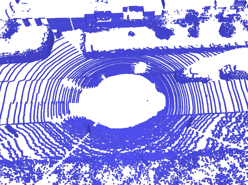
(a) Sparse LiDAR Input

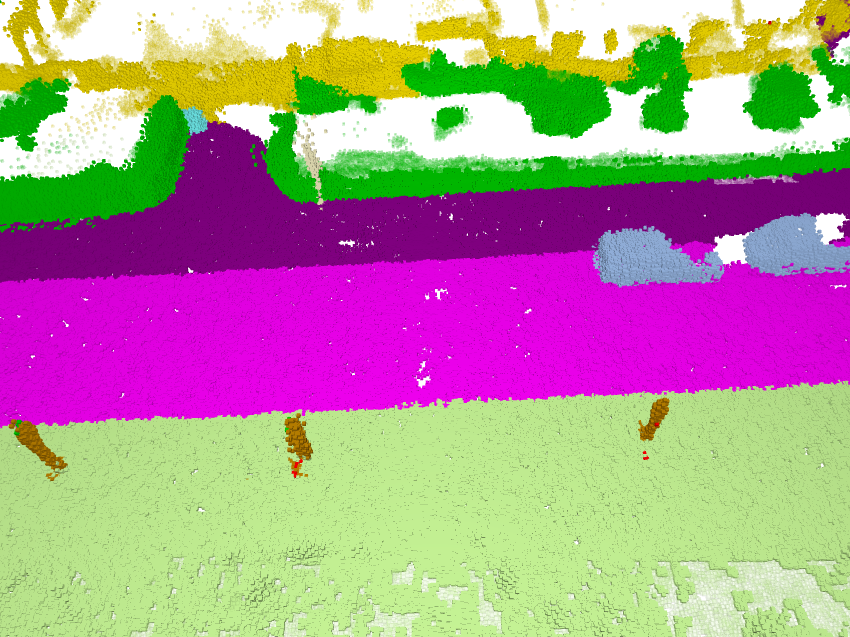
(b) Dense Semantic Estimation

Figure 1: DiffSSC estimates unseen points with semantics (b) from raw LiDAR point clouds (a). The unknown areas, as defined by ground truth, are visualized at 20$\%$ opacity in (b).

However, most traditional SSC methods are limited to learning the prior distribution of data directly, i.e., training a network to estimate the target output directly from partial inputs. Another approach to learning prior distributions is to estimate residuals. Denoising Diffusion Probabilistic Models (DDPMs) gradually introduce noise into the data in the forward diffusion process and employ a denoiser to learn how to remove these noise residuals. The denoiser iteratively predicts and removes noise, allowing the model to recover high-quality data from pure noise. This mechanism effectively learns the prior distribution of the data, which has the potential to be applied in SSC tasks.

In this work, we propose DiffSSC, a novel SSC approach leveraging DDPMs. As shown in Fig. 1, our method jointly estimates missing geometry and semantics from a scene using raw sparse LiDAR point clouds. During training, the model learns the prior distribution by predicting residuals at different noise intensity levels. These multi-level noisy data are generated from ground truth using data augmentation. In the inference stage, the sparse semantic logits serve as conditional input, and the model generates a dense and semantic scene from pure Gaussian noise through a multi-step Markov process. We model both the point and semantic spaces, designing the forward diffusion and reverse denoising processes to enable the model to learn the scene prior to the semantic point cloud representation. In summary, our key contributions are:

• We utilize DDPMs for the SSC task, introducing a residual-learning mechanism compared to traditional approaches that directly estimate the complete scene from partial input.

• We separately model the point and semantic spaces to adapt to the diffusion process.

• Our approach operates directly on the point cloud, avoiding quantization errors and reducing memory usage, while making it a more efficient method for LiDAR point clouds.

• We design local and global regularization losses to stabilize the learning process.

II Related Work

II-A LiDAR Perception

LiDAR is widely used in various autonomous agents for collecting 3D point clouds from the environment. In the past, extensive research was dedicated to employing LiDAR for odometry [1] and mapping [2, 3]. Given the inherent challenges of LiDAR, including data sparsity, noise, and outliers, researchers concentrated on developing filtering algorithms [4] and robust point cloud registration [5] to achieve accurate and efficient LiDAR-SLAM systems. With the advent of deep learning, LiDAR data began to be leveraged for object detection [6] and semantic segmentation [7]. Additionally, unlike dense representations such as images, the sparse nature of LiDAR point clouds presents unique challenges for models. To address these challenges, some researchers focus on estimating the gaps between sweeps and occluded regions from sparse point clouds. This has led to the development of semantic scene completion, an emerging technique in LiDAR perception.

II-B Semantic Scene Completion (SSC)

The task of completion has a long research history. Early efforts in this field focused on filling small holes in shapes to enhance model quality, typically employing continuous energy minimization techniques [8]. With the advent of deep learning, approaches evolved to enable networks to learn extensive geometric shape properties [9], allowing to estimate of entire models from partial inputs. In contrast to shape completion, semantic scene completion (SSC) [10] presents a significantly more complex challenge. Scenes exhibit more intricate geometric structures and encompass a wider range of semantic categories. SSCNet [11] represents the pioneering work that formally defined this task. Since its introduction, various input data modalities, such as occupancy grids [12], images [13], and LiDAR-camera fusion [14], have been explored. Additionally, a wide array of methodologies, including point-voxel mapping [15], transformers [16], bird’s-eye view (BEV) assistance [17], and knowledge distillation [18], have been employed to advance the state of the art in this domain. However, these approaches generally operate on voxelized grids, which poses specific challenges for LiDAR point clouds, as voxelization can introduce quantization errors, leading to a loss of resolution and increased memory usage. In this work, we operate directly on point clouds, offering a more efficient method for handling LiDAR data.

II-C Denoising Diffusion Probabilistic Models

Although diffusion models were originally discovered and proposed in the field of physics, DDPMs [19] was the first to apply this method to generative models. In subsequent research, Rombach et al. [20] introduced latent diffusion models, where the diffusion process is performed in the latent space of the image. This significantly improved computational efficiency and reduced resource consumption, enabling the generation of high-quality and high-resolution images, marking a breakthrough in the field of artistic creation. Beyond artistic applications, several works [21, 22] have also adapted diffusion models for LiDAR perception. These approaches typically project 3D data onto image-based representations, such as range images, allowing methods developed for image domains to be directly applied. Notably, due to the higher demands for accuracy in robotics, controlling the generative process to achieve realistic results remains a significant challenge when applying diffusion models in this field. The recent LiDiff [23] directly applies diffusion models to 3D point clouds for scene completion. However, it still lacks the capability to model and process semantics simultaneously. In this work, we apply DDPM to semantic scene completion, to generate dense and accurate semantic scenes.

III Methodology

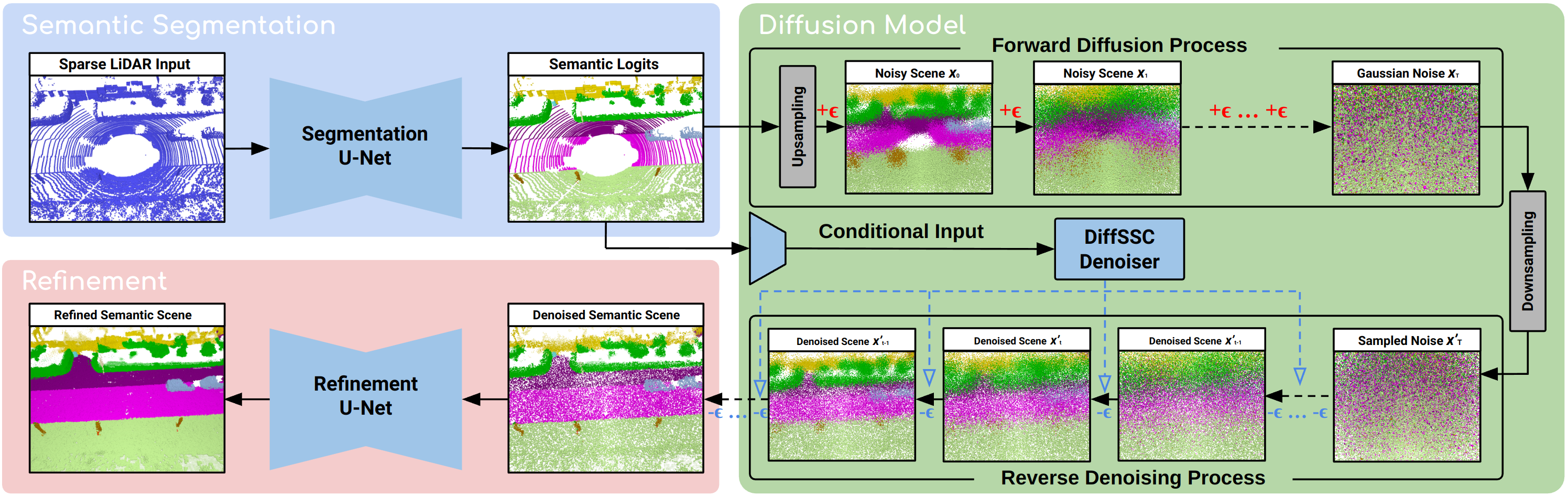
Figure 2: The overall pipeline of DiffSSC. The raw LiDAR point cloud is semantically segmented using Cylinder3D [7] to generate initial semantic logits. The semantic point cloud is then upsampled, increasing point density for the diffusion process. These duplicated points undergo forward diffusion and reverse denoising, refining their positions and semantic labels. The original semantic point cloud serves as a conditional input, guiding the generation of points in gaps and occluded areas. To further enhance the generated scene, we introduce a refinement model based on MinkUNet [24, 25, 26, 27], which increases the density of the point cloud.

Given a raw LiDAR point cloud, our objective is to estimate a more complete semantic point cloud, including unobserved points with associated semantic labels within gaps and occluded regions. As illustrated in the Fig. 2, we build a diffusion model based on LiDiff [23], supported by a semantic segmentation module and a refinement module. First, the raw LiDAR point cloud is semantically segmented using a Cylinder3D [7] to generate initial semantic logits. Next, we upsample the semantic point cloud to increase point density for the diffusion process. The duplicated semantic points undergo a forward diffusion and a reverse denoising process to adjust their positions and semantics. Notably, the semantic point cloud also serves as a conditional input for the diffusion model, guiding the generation process. The generated scene includes semantic points located in gaps and occluded areas. To further enhance the quality of the generated scene, we designed a refinement model based on MinkUnet [24, 25, 26, 27] to densify the point cloud.

III-A Denoising Diffusion Probabilistic Models (DDPMs)

Ho et al. [19] introduced DDPMs to produce high-quality images through iterative denoising from Gaussian noise. This promising capability is driven by a residual learning mechanism that efficiently captures the data distribution. Specifically, the process begins with a forward diffusion step, during which noise is gradually added to the target data over $T$ steps. The model is then trained to predict the noise added at each step. By predicting and removing noise at time step $t$, the model generates results that closely approximate the raw data distribution.

III-A1 Forward Diffusion Process

Assuming a sample $\bm{x}_{0}\sim q(\bm{x})$ from a target data distribution, the diffusion process gradually adds noise to $\bm{x}_{0}$ over $T$ steps, producing a sequence $\bm{x}_{1},\ldots,\bm{x}_{T}$. When $T$ is large enough, $q(\bm{x}_{T})$ is approximately equal to a normal distribution $\mathcal{N}(\bm{0},\bm{I})$. The intensity of noise added at each step is defined by the noise factors $\beta_{1},\ldots,\beta_{T}$, which significantly influences the performance of the diffusion model. Specifically, at step $t$, Gaussian noise amplified by $\beta_{t}$ is sampled and added to $\bm{x}_{t-1}$. In  [19], the noise parameter $\beta_{t}$ is determined using a linear schedule, starting from an initial value $\beta_{0}$ and linearly increasing over $T$ steps to a final value $\beta_{T}$. Subsequently, several improved noise schedules have been proposed, such as the cosine schedule [28] and the sigmoid schedule [29]. Due to the inefficiency of adding noise step by step, especially during training, where the noise from different steps can be shuffled, one can simplify this process by sampling $\bm{x}_{t}$ from $\bm{x}_{0}$ without computing the intermediate steps $\bm{x}_{1},\ldots,\bm{x}_{t-1}$. To achieve this, Ho et al. [19] define $\alpha_{t}=1-\beta_{t}$ and $\bar{\alpha}_{t}=\prod_{i=1}^{t}\alpha_{i}$, allowing $\bm{x}_{t}$ to be sampled as:

$$\bm{x}_{t}=\sqrt{\bar{\alpha}_{t}}\bm{x}_{0}+\sqrt{1-\bar{\alpha}_{t}}\bm{\epsilon}$$ (1)

where $\bm{\epsilon}\sim\mathcal{N}(0,I)$. It is important to note that as $T$ is large enough, $q(\bm{x}_{T})$ approaches $\mathcal{N}(\bm{0},\bm{I})$ because $\bar{\alpha}_{T}$ tends to zero.

III-A2 Reverse Denoising Process

The denoising process reverses diffusion and aim to recover the original sample $\bm{x}_{0}$ from Gaussian noise. This is accomplished by a denoiser, which predicts and removes the noise at each step. The reverse diffusion step can be formulated as:

$$\bm{x}_{t-1}=\bm{x}_{t}-\frac{1-\alpha_{t}}{\sqrt{1-\bar{\alpha}_{t}}}\bm{\epsilon}_{\theta}(\bm{x}_{t},t)+\frac{1-\bar{\alpha}_{t-1}}{1-\alpha_{t}}\beta_{t}\mathcal{N}(\bm{0},\bm{I})$$ (2)

where $\bm{\epsilon}_{\theta}(\bm{x}_{t},t)$ is the noise predicted from $\bm{x}_{t}$ at step $t$. The process of generating the original data can be formulated as a Markov process that repeatedly calls the denoiser until $t=0$. At this point, the model generates a result that approximates $\bm{x}_{0}$. Due to the denoiser effectively learning the high quality of the data distribution $q(\bm{x}_{T})$, the generated samples are of similarly high quality.

While the denoising process generates samples with quality similar to the dataset, it only produces random samples. Hence, the denoising process cannot control the generation of specific desired data, which poses challenges for certain downstream applications.  [28] addresses this issue by introducing conditional inputs to guide the generation process. This advancement allows us to apply diffusion models to tasks like SSC.

III-B Diffusion Semantic Scene Completion

Regarding the principles of DDPMs, we introduce its application in SSC. To focus on the main components, we assume that primary semantic segmentation has been obtained using Cylinder3D. In the context of the diffusion model, the input is a partial semantic point cloud $\mathcal{X}=\{\bm{x}^{1},\dots,\bm{x}^{N}\}$, where each semantic point $\bm{x}^{i}$ is a tuple of a point position and a semantic probability vector $(\bm{p}^{i},\bm{s}^{i})$. Here, $\bm{p}^{i}\in\mathbb{R}^{3}$ represents the 3D coordinates, and $\bm{s}^{i}\in\Delta^{C-1}=\{\bm{s}\in\mathbb{R}^{C}\mid\sum_{j=1}^{C}s^{j}=1,s^{j}\geq 0\}$ lies in the standard $(C-1)$-dimensional simplex, assuming there are $C$ classes in total. The output estimates complete point cloud $\hat{\mathcal{Y}}=\{\hat{\bm{y}}^{1},\dots,\hat{\bm{y}}^{M}\}$. We generate the reference $\mathcal{Y}=\{\bm{y}^{1},\dots,\bm{y}^{M}\}$ by fusing multiple frames with ground-truth semantic labels and then taking the corresponding region as the input scan $\mathcal{X}$. Our goal is to make the estimated $\hat{\mathcal{Y}}$ as close as possible to the ground truth $\mathcal{Y}$.

As mentioned in Sec. I, by learning scene priors, the model gains the ability to estimate a complete scene (posterior) from partial observations (likelihood). The diffusion model efficiently learns the distribution of the ground truth data, acquiring knowledge of the scene prior. To achieve this, we gradually add noise to the ground truth $\mathcal{Y}$, resulting in $\mathcal{Y}_{1},\dots,\mathcal{Y}_{T}$, until $\mathcal{Y}_{T}$ approximates a Gaussian distribution. This form of data augmentation can be simplified using Eq. 1. However, this approach does not directly apply to semantic scene completion. In Eq. 1, the diffusion process is defined as a combined distribution of the sample $\bm{x}_{0}$ and global noise $\bm{\epsilon}\sim\mathcal{N}(0,I)$, with coefficients $\sqrt{\bar{\alpha}_{t}}$ and $\sqrt{1-\bar{\alpha}_{t}}$ controlling the ratio of noise and sample at different time steps. This mechanism works well in shape completion, as the shapes generally approximate a 3D Gaussian distribution. However, the data distribution in large-scale scenes deviates significantly from Gaussianity, particularly due to varying data ranges across different axes. Applying global noise to the entire scene point cloud as a single entity can obscure important details. Therefore, we use the local point diffusion proposed by Nunes et al. [23], which reformulates the diffusion process as a noise offset $\bm{\epsilon}\in\mathbb{R}^{3+C}$ added locally to each point $\bm{y}^{m}\in\mathcal{Y}$, as shown in the following equation:

$$\bm{y}_{t}^{m}=\bm{y}^{m}+\sqrt{1-\bar{\alpha}_{t}}\bm{\epsilon}$$ (3)

where $\bm{\epsilon}$ is not an isotropic Gaussian distribution, because of different scaling for 3D positions and semantics.

Although training on ground truth allows the model to generate high-quality results, the process remains inherently uncontrollable. The goal of SSC is to predict a complete scene from partial input, rather than randomly generating scenes. Therefore, during training, we also use the partial semantic point cloud $\mathcal{X}$ as a conditional input, feeding it into the model to guide the point cloud generation. During training, we load a random step $t\in[0,T]$ at each iteration and compute the corresponding $\mathcal{Y}_{t}$ using Eq. 3. The model is trained to estimate the noise at various intensities with the following loss:

$$L_{2}(\mathcal{Y}_{t},\mathcal{X},t)=\left\lVert\bm{\epsilon}-\bm{\epsilon}_{\theta}(\mathcal{Y}_{t},\mathcal{X},t)\right\rVert^{2}$$ (4)

In traditional loss design, the predicted result is directly compared to the ground truth. However, our approach uses residual learning, where the model’s output is compared to the residual. Therefore, to generate the final scene, the estimated noise must be removed from the noised scene.

During inference, the model begins denoising from Gaussian noise and iteratively predicts and removes the noise in the samples, ultimately generating a dense semantic scene. Since ground truth is not available during inference, Gaussian noise is generated from $\mathcal{X}$. We duplicate the points in $\mathcal{X}$ to match the quantity in the ground truth, ensuring that there are enough points to perform the diffusion process using Eq. 3. Note that the denoiser also takes the partial semantic point cloud $\mathcal{X}$ as a condition to guide the generation process.

III-C Denoiser Design and Regularization

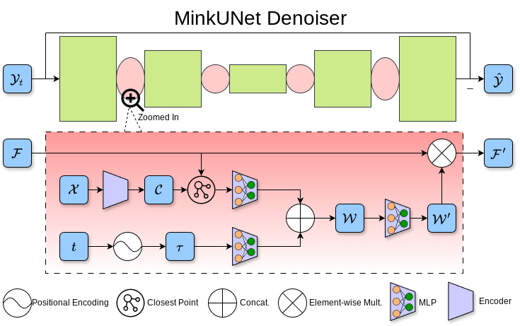
Figure 3: Architecture of our MinkUNet Denoiser. The conditional input, detailed in the red area, is inserted between each layer of denoiser to guide the generation of point cloud.

As shown in Fig. 3, the denoiser is based on the MinkUNet architecture [24, 25, 26, 27]. Given the feature $\mathcal{F}$ extracted from a layer of MinkUNet, we integrate the conditional input and step information between layers to obtain the fused feature $\mathcal{F}^{\prime}$. The raw semantic point cloud $\mathcal{X}$ is encoded as a conditional input $\mathcal{C}$ using the same MinkUNet encoder. To embed the most relevant conditional input into the feature space, a closest point algorithm is employed to effectively align the conditional input with the features. Simultaneously, the step $t$ is encoded as $\tau$ using sinusoidal positional encodings. After passing through an MLP individually, the conditional input and step information are concatenated to form the weight $\mathcal{W}$. To align the dimensions with the feature $\mathcal{F}$, $\mathcal{W}$ is processed through an MLP to produce $\mathcal{W}^{\prime}$. Finally, $\mathcal{W}^{\prime}$ and $\mathcal{F}$ are element-wise multiplied to form the refined feature $\mathcal{F}^{\prime}$, which is then passed to the next layer.

As proposed by Nunes et al. [23], the regularization loss consists of a local term focusing on each point and a global term addressing the statistical characteristics. We extend this design to the semantic domain by employing an $L_{2}$ loss between the added noise and the model’s predictions, along with losses for the mean $\mu_{\epsilon}$ and variance $\sigma_{\epsilon}$ to regulate the global statistical properties. Thus, the overall loss is formulated as follows:

$$L=L_{2}+\lambda(L_{\text{mean}}+L_{\text{var}})=L_{2}+\lambda(\mu_{\epsilon}^{2}+(\sigma_{\epsilon}-1)^{2})$$ (5)

where $L_{\text{diff}}$ is the regularization term focused on local features, commonly used in DDPM models, while $L_{\text{mean}}=\mu_{\epsilon}^{2}$ and $L_{\text{var}}=(\sigma_{\epsilon}-1)^{2}$ are designed to ensure the overall noise distribution aligns with a Gaussian distribution.

III-D Refinement

Inspired by Lyu et al. [30], we design a refinement and upsampling scheme based on MinkUNet to further enhance the density of the diffusion model’s output. This module predicts $k$ bias $b_{k}\in\mathbb{R}^{3}$ for each point position in the completed scene, while the semantics are propagated to the biased points. The refinement module offers a marginal improvement in scene quality, but it functions more like interpolating points in the gaps, rather than learning to predict missing geometry and semantics. The main contribution is made by the diffusion model, as will be demonstrated in the ablation study.

IV Experiment

IV-A Experiment Setup

IV-A1 Datasets

We evaluate our approach using the SemanticKITTI [31] and SSCBench-KITTI360 [32] datasets. SemanticKITTI is a widely used autonomous driving dataset that provides point-wise annotations on raw LiDAR point clouds, extending the KITTI dataset to semantic study. Additionally, it builds the SSC benchmark by accumulating annotated scans within sequences. SSCBench-KITTI360 is another SSC benchmark derived from KITTI-360 [33], featuring LiDAR scans encoded the same as SemanticKITTI. This consistency allows SSC methods evaluated on SemanticKITTI to be seamlessly transferred to the KITTI-360 scenario. However, these SSC benchmarks only use the front half of the LiDAR scan (180° LiDAR field-of-view (FoV)) as input, which is not ideal for LiDAR-centered point cloud data. To address this, we additionally incorporate the rear half of the point cloud, facilitating the evaluation of SSC approaches on LiDAR-centered data. Our model is trained and validated purely on SemanticKITTI, using sequences 00-06 for training and sequences 09-10 for validation. We evaluate our model using the official validation sets of both datasets: sequence 08 of SemanticKITTI and sequence 07 of SSCBench-KITTI360.

IV-A2 Training and Inference

To train DiffSSC on the 360^∘ LiDAR FoV, we generate the ground truth following the guidelines of SemanticKITTI. First, given the pose of each frame, we construct the global map by aggregating the semantic LiDAR sweeps within the sequence. Next, we extract the neighboring region around the key frame, specifically, a spherical area centered on the LiDAR with a radius of 60 meters. The model is trained on an NVIDIA A6000 GPU for 20 epochs. For the diffusion parameters, we employ a cosine schedule to modulate the intensity of noise at each step. Specifically, we set $\beta_{0}=3.5\times 10^{-5}$ and $\beta_{T}=0.007$, with the number of diffusion steps $T=1000$, and define $\beta_{1},\dots,\beta_{T-1}$ using the following equation.

$$\beta_{t}=\beta_{0}+\frac{1}{2}\left(1+\cos\left(\frac{t}{T}\cdot\pi\right)\right)\cdot(\beta_{T}-\beta_{0})$$ (6)

We also set the ratio of global regularization to $\lambda=5.0$.

IV-A3 Baselines

We compare our approach against LMSCNet [12], JS3C-Net [15], and LODE [34]. Both LMSCNet and JS3C-Net take the front half of the quantized LiDAR sweep as input and are evaluated in the SSC benchmark of SemanticKITTI. LODE primarily focuses on geometry completion using implicit representation. However, to demonstrate its flexibility, the authors also report results with extended semantic parsing. A common limitation among these baselines is that they are trained on point clouds within a 180^∘ LiDAR field of view. To fairly compare with our method, we split the 360^∘ LiDAR point cloud input into two halves and feed them separately into the baselines. The outputs from these two halves are then concatenated to obtain a 360^∘ result. Additionally, while these baselines have only been tested on SemanticKITTI, we also ran them on SSCBench-KITTI360 as a supplementary experiment. Since the semantic labels and overall pipeline in SSCBench-KITTI360 are consistent with SemanticKITTI, the baselines can be seamlessly applied to this dataset.

IV-A4 Evaluation Metrics and Pipeline

Despite our task being set in a 360^∘ LiDAR point cloud completion context, we aimed to retain the baseline settings as closely as possible to ensure a fair comparison. In the raw SSC setting of SemanticKITTI, the scene is limited to a cuboid region, represented in the LiDAR’s local coordinate system as: $V_{\text{kitti}}=\{(x,y,z)\mid x\in[0,51.2]\text{ m},y\in[-25.6,+25.6]\text{ m},z\in[-3.2,+3.2]\text{ m}\}$, which corresponds to a region associated only with the LiDAR’s $[-90^{\circ},+90^{\circ}]$ FoV. To cover the full $[-180^{\circ},+180^{\circ}]$ panoramic range while preserving spatial symmetry, we selected an evaluation region within the LiDAR’s local coordinate system defined as: $V_{\text{ours}}=\{(x,y,z)\mid x\in[-51.2,51.2]\text{ m},y\in[-25.6,+25.6]\text{ m},z\in[-3.2,+3.2]\text{ m}\}$.

We directly used the baselines’ official code and checkpoints to predict the front and rear parts of the scene, with each part of the LiDAR sweep input separately. Although the baselines were trained only on the front part of the scene, the statistical characteristics of LiDAR data in the front and rear regions are similar, suggesting that a model trained using only the front half of the data remains effective for the rear region as well. Although our ground truth generation covers a spherical region with a radius of 60 meters centered on the LiDAR, we limited our evaluation to the region predicted by the baselines. Additionally, the unknown areas defined by the raw dataset were mapped into $V_{\text{ours}}$ using known poses, and these unknown areas were excluded from the evaluation.

Although our method operates directly on point clouds, point clouds cannot represent continuous regions in space, which makes direct evaluation using traditional IoU challenging. Therefore, we voxelized our results and used traditional IoU for scene completion and mIoU for semantic scene completion evaluation. While this introduces quantization error and potentially degrades our model’s performance, it aligns with the baseline settings and preserves their performance for a fair comparison.

IV-B Main Results

Based on the experimental setting described above, we present the results in Tab. I. Our results include the direct predictions from DiffSSC and the outcomes after refinement. We do the ablation study without the diffusion model, which means directly refining the output of Cylinder3D. We also report the results of baselines as a comparison.

TABLE I: Quantitative results on SemanticKITTI and SSCBench-KITTI360

Method	Reference	SemanticKITTI		SSCBench-KITTI360
		IoU(SC)	mIoU(SSC)	IoU(SC)	mIoU(SSC)
LMSCNet [12]	3DV’20	48.24	15.43	33.64	13.47
JS3C-Net [15]	AAAI’21	51.32	21.38	35.57	16.95
LODE [34]	ICRA’23	50.61	18.22	38.24	15.39
Cylinder3D(refined)	-	23.36	7.63	20.66	7.21
DiffSSC	-	49.38	22.67	36.76	17.34
DiffSSC(refined)	-	57.03	25.87	40.72	18.51

Best and second best results are highlighted.

Figure 4: Qualitative results on SemanticKITTI and SSCBench-KITTI360. The 19 classes are shown without empty spaces. The estimated points that are located at the unknown region are visualized with $20\%$ opacity.

Qualitative results are presented in Fig.4. To emphasize the advantages of our approach, which operates directly on point clouds, we visualize samples from both the SemanticKITTI and SSCBench-KITTI360 datasets in point cloud form. For voxel-based methods, the point cloud is generated by sampling the center point of each occupied voxel. As shown in Fig.4, our DiffSSC model predicts more accurate semantic segmentation of the background and provides a more precise representation of the foreground shapes. Furthermore, the voxel-based baselines, which estimate the scene using two halves of a LiDAR sweep, exhibit discontinuous predictions at the boundary between the front and rear segments.

IV-C Model Analysis

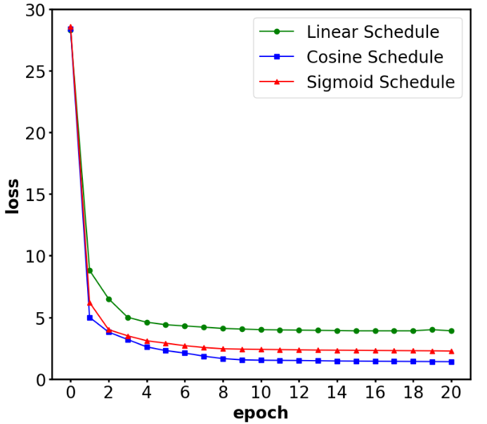
(a) Noise schedule

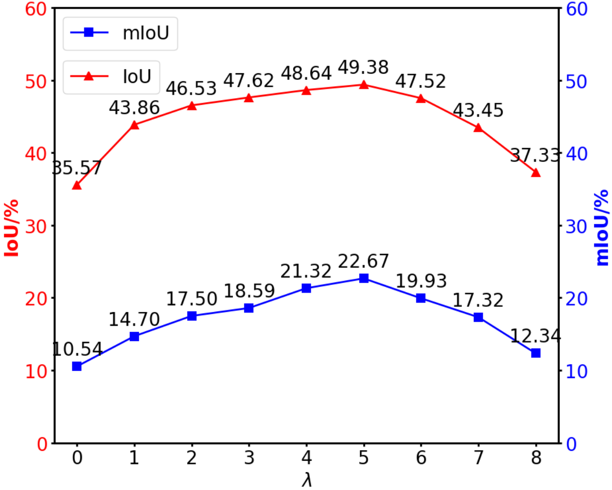
(b) Ratio of global regularization

Figure 5: Hyperparameter study for the model’s performance

IV-C1 Noise Schedule

As mentioned in Sec.III, the noise schedule determines the intensity of noise added at each step, commonly including linear, cosine, and sigmoid schedules. We conducted a series of experiments to identify the most effective noise schedule for the SSC task. In Fig.5(a), we present the training curves sampled at each epoch, highlighting the convergence patterns for each schedule. Additionally, we compare the output of DiffSSC without refinement using each noise schedule in Tab.II, providing insights into their impact. The linear schedule, the simplest, was primarily used in early research. It shows slow and stable convergence, and its performance is significantly lower than that of the other two schedules. The cosine schedule, an improved function, introduces noise more gradually at the beginning and end, with a faster increase in the middle, balancing faster convergence with high final generation quality. The sigmoid schedule shares similarities with the cosine schedule, featuring an S-shaped curve but offering more precise control over the noise introduction, theoretically providing even greater potential. As a result, the cosine schedule converges significantly faster than the linear one. Although the sigmoid schedule does not converge as quickly as the cosine schedule, it is still noticeably faster than the linear schedule. They perform comparably, though the sigmoid schedule is slightly weaker than the cosine schedule. Therefore, in our main results, we adopted the cosine schedule.

TABLE II: Model’s performance based on different noise schedule functions

Noise Schedule	SemanticKITTI		SSCBench-KITTI360
	IoU(SC)	mIoU(SSC)	IoU(SC)	mIoU(SSC)
Linear	45.26	19.02	33.32	14.99
Sigmoid	48.29	22.48	36.24	16.55
Cosine	49.38	22.67	36.76	17.34

Best and second best results are highlighted.

IV-C2 Regularization

We also investigated the model’s performance on SemanticKITTI under different ratios of global regularization, as shown in Fig. 5(b). When $\lambda=0$, indicating the use of only local $L_{2}$ regularization without global regularization, the model exhibited the worst performance, highlighting the benefits of incorporating global regularization. As the ratio increases, the model’s performance improves, peaking at $\lambda=5$ before declining. This suggests that excessive global regularization can constrain the model’s ability to generate finer details.

V Conclusions and Outlook

We proposed DiffSSC, a novel SSC approach based on a diffusion model. It takes raw LiDAR point clouds as input and jointly predicts missing points along with their semantic labels, thereby extending the application boundaries of diffusion models. We evaluated our method on two autonomous driving datasets, achieving performance that surpasses the state-of-the-art. In future work, we will explore methods to enhance inference speed by streamlining the step-by-step inference process, enabling the application of diffusion models  [35]. Regarding the impact of noise schedules, we will also explore more complex yet efficient scheduling mechanisms, such as adaptive schedules [36].

References

- [1] J. Quenzel and S. Behnke, “Real-time multi-adaptive-resolution-surfel 6D lidar odometry using continuous-time trajectory optimization,” in Proceedings of the IEEE/RSJ International Conference on Intelligent Robots and Systems (IROS). IEEE, 2021, pp. 5499–5506.
- [2] D. Droeschel and S. Behnke, “Efficient continuous-time slam for 3D lidar-based online mapping,” in Proceedings of the IEEE International Conference on Robotics and Automation (ICRA). IEEE, 2018, pp. 5000–5007.
- [3] X. Zhong, Y. Pan, J. Behley, and C. Stachniss, “SHINE-Mapping: Large-Scale 3D Mapping Using Sparse Hierarchical Implicit Neural Representations,” in Proceedings of the IEEE International Conference on Robotics and Automation (ICRA), 2023.
- [4] R. B. Rusu and S. Cousins, “3D is here: Point cloud library (pcl),” in Proceedings of the IEEE International Conference on Robotics and Automation (ICRA). IEEE, 2011, pp. 1–4.
- [5] I. Vizzo, T. Guadagnino, B. Mersch, L. Wiesmann, J. Behley, and C. Stachniss, “KISS-ICP: In Defense of Point-to-Point ICP – Simple, Accurate, and Robust Registration If Done the Right Way,” IEEE Robotics and Automation Letters (RA-L), vol. 8, no. 2, pp. 1029–1036, 2023.
- [6] L. Nunes, L. Wiesmann, R. Marcuzzi, X. Chen, J. Behley, and C. Stachniss, “Temporal Consistent 3D LiDAR Representation Learning for Semantic Perception in Autonomous Driving,” in Proceedings of the IEEE Conference on Computer Vision and Pattern Recognition (CVPR), 2023.
- [7] X. Zhu, H. Zhou, T. Wang, F. Hong, Y. Ma, W. Li, H. Li, and D. Lin, “Cylindrical and asymmetrical 3D convolution networks for lidar segmentation,” arXiv preprint arXiv:2011.10033, 2020.
- [8] M. Kazhdan, M. Bolitho, and H. Hoppe, “Poisson surface reconstruction,” in Proceedings of the Eurographics Symposium on Geometry Processing (SGP), vol. 7, no. 4, 2006.
- [9] A. Dai, C. Ruizhongtai Qi, and M. Nießner, “Shape completion using 3D-encoder-predictor cnns and shape synthesis,” in Proceedings of the IEEE Conference on Computer Vision and Pattern Recognition (CVPR), 2017, pp. 5868–5877.
- [10] L. Roldão, R. de Charette, and A. Verroust-Blondet, “3D semantic scene completion: A survey,” International Journal of Computer Vision (IJCV), vol. 130, no. 8, pp. 1978–2005, 2022.
- [11] S. Song, F. Yu, A. Zeng, A. X. Chang, M. Savva, and T. Funkhouser, “Semantic scene completion from a single depth image,” in Proceedings of the IEEE Conference on Computer Vision and Pattern Recognition (CVPR), 2017, pp. 1746–1754.
- [12] L. Roldao, R. de Charette, and A. Verroust-Blondet, “LMSCNet: Lightweight multiscale 3D semantic completion,” in Proceedings of the International Conference on 3D Vision (3DV), 2020, pp. 111–119.
- [13] A.-Q. Cao and R. de Charette, “MonoScene: Monocular 3D semantic scene completion,” in Proceedings of the IEEE Conference on Computer Vision and Pattern Recognition (CVPR), 2022, pp. 3991–4001.
- [14] H. Cao and S. Behnke, “SLCF-Net: Sequential LiDAR-camera fusion for semantic scene completion using a 3D recurrent U-Net,” in Proceedings of the IEEE International Conference on Robotics and Automation (ICRA), 2024, pp. 2767–2773.
- [15] X. Yan, J. Gao, J. Li, R. Zhang, Z. Li, R. Huang, and S. Cui, “Sparse single sweep LiDAR point cloud segmentation via learning contextual shape priors from scene completion,” in Proceedings of the National Conference on Artificial Intelligence (AAAI), vol. 35, no. 4, 2021, pp. 3101–3109.
- [16] Y. Li, Z. Yu, C. Choy, C. Xiao, J. M. Alvarez, S. Fidler, C. Feng, and A. Anandkumar, “Voxformer: Sparse voxel transformer for camera-based 3D semantic scene completion,” in Proceedings of the IEEE Conference on Computer Vision and Pattern Recognition (CVPR), 2023, pp. 9087–9098.
- [17] R. Cheng, C. Agia, Y. Ren, X. Li, and L. Bingbing, “S3cnet: A sparse semantic scene completion network for lidar point clouds,” in Proceedings of Machine Learning Research (PMLR). PMLR, 2021, pp. 2148–2161.
- [18] X. Fan, H. Luo, X. Zhang, L. He, C. Zhang, and W. Jiang, “Scpnet: Spatial-channel parallelism network for joint holistic and partial person re-identification,” in Proceedings of the Asian Conference on Computer Vision (ACCV). Springer, 2019, pp. 19–34.
- [19] J. Ho, A. Jain, and P. Abbeel, “Denoising diffusion probabilistic models,” arXiv preprint arxiv:2006.11239, 2020.
- [20] R. Rombach, A. Blattmann, D. Lorenz, P. Esser, and B. Ommer, “High-resolution image synthesis with latent diffusion models,” in Proceedings of the IEEE Conference on Computer Vision and Pattern Recognition (CVPR), 2022, pp. 10 684–10 695.
- [21] K. Nakashima and R. Kurazume, “Lidar data synthesis with denoising diffusion probabilistic models,” arXiv preprint arXiv:2309.09256, 2023.
- [22] V. Zyrianov, X. Zhu, and S. Wang, “Learning to generate realistic lidar point clouds,” in Proceedings of the European Conference on Computer Vision (ECCV). Springer, 2022, pp. 17–35.
- [23] L. Nunes, R. Marcuzzi, B. Mersch, J. Behley, and C. Stachniss, “Scaling Diffusion Models to Real-World 3D LiDAR Scene Completion,” in Proceedings of the IEEE Conference on Computer Vision and Pattern Recognition (CVPR), 2024.
- [24] C. Choy, J. Gwak, and S. Savarese, “4d spatio-temporal convnets: Minkowski convolutional neural networks,” in Proceedings of the IEEE Conference on Computer Vision and Pattern Recognition (CVPR), 2019, pp. 3075–3084.
- [25] C. Choy, J. Park, and V. Koltun, “Fully convolutional geometric features,” in Proceedings of the IEEE International Conference on Computer Vision (ICCV), 2019, pp. 8958–8966.
- [26] C. Choy, J. Lee, R. Ranftl, J. Park, and V. Koltun, “High-dimensional convolutional networks for geometric pattern recognition,” in Proceedings of the IEEE Conference on Computer Vision and Pattern Recognition (CVPR), 2020.
- [27] J. Gwak, C. B. Choy, and S. Savarese, “Generative sparse detection networks for 3D single-shot object detection,” in Proceedings of the European Conference on Computer Vision (ECCV), 2020.
- [28] A. Q. Nichol and P. Dhariwal, “Improved denoising diffusion probabilistic models,” in Proceedings of the IEEE International Conference on Machine Learning (ICML). PMLR, 2021, pp. 8162–8171.
- [29] D. Kingma, T. Salimans, B. Poole, and J. Ho, “Variational diffusion models,” Advances in Neural Information Processing Systems (NIPS), vol. 34, pp. 21 696–21 707, 2021.
- [30] Z. Lyu, Z. Kong, X. Xu, L. Pan, and D. Lin, “A conditional point diffusion-refinement paradigm for 3D point cloud completion,” arXiv preprint arXiv:2112.03530, 2021.
- [31] J. Behley, M. Garbade, A. Milioto, J. Quenzel, S. Behnke, C. Stachniss, and J. Gall, “SemanticKITTI: A dataset for semantic scene understanding of LiDAR sequences,” in Proceedings of the IEEE International Conference on Computer Vision (ICCV), 2019.
- [32] Y. Li, S. Li, X. Liu, M. Gong, K. Li, N. Chen, Z. Wang, Z. Li, T. Jiang, F. Yu et al., “Sscbench: Monocular 3D semantic scene completion benchmark in street views,” arXiv preprint arXiv:2306.09001, 2023.
- [33] Y. Liao, J. Xie, and A. Geiger, “Kitti-360: A novel dataset and benchmarks for urban scene understanding in 2D and 3D,” IEEE Transactions on Pattern Analysis and Machine Intelligence, vol. 45, no. 3, pp. 3292–3310, 2022.
- [34] P. Li, R. Zhao, Y. Shi, H. Zhao, J. Yuan, G. Zhou, and Y.-Q. Zhang, “Lode: Locally conditioned eikonal implicit scene completion from sparse lidar,” in Proceedings of the IEEE International Conference on Robotics and Automation (ICRA). IEEE, 2023, pp. 8269–8276.
- [35] C. Lu, Y. Zhou, F. Bao, J. Chen, C. Li, and J. Zhu, “Dpm-solver: A fast ode solver for diffusion probabilistic model sampling in around 10 steps,” Advances in Neural Information Processing Systems (NIPS), vol. 35, pp. 5775–5787, 2022.
- [36] A. Jabri, D. Fleet, and T. Chen, “Scalable adaptive computation for iterative generation,” arXiv preprint arXiv:2212.11972, 2022.