One and two sample Dvoretzky-Kiefer-Wolfowitz-Massart type inequalities for differing underlying distributions

Abstract

Kolmogorov-Smirnov (KS) tests rely on the convergence to zero of the KS-distance $d(F_{n},G)$ in the one sample case, and of $d(F_{n},G_{m})$ in the two sample case. In each case the assumption (the null hypothesis) is that $F=G$, and so $d(F,G)=0$. In this paper we extend the Dvoretzky-Kiefer-Wolfowitz-Massart inequality to also apply to cases where $F\neq G$, i.e. when it is possible that $d(F,G)>0$.

[1]organization=School of Engineering and Physical Sciences, University of Lincoln, addressline=Brayford pool, city=Lincoln, postcode=LN6 7TS, country=United Kingdom

1 Introduction

Let $X_{1},\dots,X_{n}$ and $Y_{1},\dots,Y_{m}$ denote samples of univariate i.i.d. random variables with continuous underlying cumulative distributions $F(x)$ and $G(x)$ respectively. Denoting the indicator function $I(X_{i}\leq x)$, which returns 1 if $X_{i}\leq x$ and zero otherwise, the corresponding empirical distributions $F_{n}(x):=\frac{1}{n}\sum_{i=1}^{n}I(X_{i}\leq x)$ and $G_{m}(x):=\frac{1}{m}\sum_{i=1}^{m}I(Y_{i}\leq x)$ are step functions that approximate $F(x)$ and $G(x)$ for sample size $n$ and $m$ respectively. The Kolmogorov-Smirnov (KS) distance, for instance $d(F_{n},F):=\sup_{x}|F_{n}(x)-F(x)|$, is a sup-norm metric defined between two distributions, which takes values in $[0,1]$, and which quantifies the similarity of these distributions. KS-type statistical hypothesis tests are based on a number of related theorems quantifying the convergence to zero with sample size of $d(F_{n},G)$ in the one sample case, and of $d(F_{n},G_{m})$ in the two sample case for $F=G$ [and so $d(F,G)=0$]. In this paper, we find an analogous convergence to non-zero values of both $d(F_{n},G)$ [Proposition 1], and $d(F_{n},G_{m})$ [Propositions 2a and 2b] in the case that $F\neq G$, so that $d(F,G)>0$.

2 Convergence to zero

One sample KS-tests were originally performed using a theorem by Kolmogorov (1933) on the asymptotic convergence of $d(F_{n},F)$ to zero. Under the assumption that $F(x)$ is continuous, this states that

$$\lim_{n\to\infty}\text{Prob}\left(\sqrt{n}d(F_{n},F)\leq z\right)=L(z),$$ (1)

where $L(z)$ is given by

$$L(z)=1-2\sum_{\nu=1}^{\infty}(-1)^{\nu-1}e^{-2\nu^{2}z^{2}}=\frac{\sqrt{2\pi}}{z}\sum_{\nu=1}^{\infty}e^{-(2\nu-1)^{2}\pi^{2}/8z^{2}}.$$ (2)

As usual, the corresponding $p$-value, $p\approx 1-L[\sqrt{n}d(F_{n},F)]$, represents the prior probability of obtaining a value at least as extreme as $d(F_{n},F)$, given the null hypothesis that the data $X_{1},\dots,X_{n}$ is drawn from distribution $F$. However this is an estimate which only becomes exact in the large sample size limit, $n\to\infty$. As sample sizes may not in practice be infinite, this one-sample test has largely been superseded by a test using a non-asymptotic theorem by Dvoretzky, Kiefer, and Wolfowitz (1956), which was later refined by Massart (1990). The DKWM inequality states that

$$\text{Prob}\left[\sqrt{n}d(F_{n},F)>z\right]\ \leq\ 2e^{-2z^{2}},$$ (3)

and holds for all $z$ and $n$. This provides a sharp upper bound to the $p$-value, $p\leq 2\exp\left[-2nd(F_{n},F)^{2}\right]$. Note that although this holds for all $z$, it may be said to have a ”useful range” of $z\geq\sqrt{(\log 2)/2}$ or equivalently $d(F_{n},F)\geq\sqrt{\log 2/(2n)}$, as outside of this range the probability upper bound is greater than unity.

Two-sample tests were traditionally performed using Smirnov’s two-sample asymptotic convergence theorem (Smirnov, 1939; Feller, 1948). This states that if $F$ and $G$ are the same continuous distribution, then

$$\lim_{N\to\infty}\text{Prob}\left(\sqrt{N}d(F_{n},G_{m})\leq z\right)=L(z),$$ (4)

where $N:=nm/(n+m)$, and where the limit is understood to be taken such that the ratio $n/m$ tends to a constant. The corresponding $p$-values, $p\approx 1-L\left[\sqrt{N}d(F_{n},G_{m})\right]$, are prior probabilities of obtaining a value at least as extreme as $d(F_{n},G_{m})$, given the null hypothesis, continuous $F=G$. In the same manner as Kolmogorov’s one sample $p$-values, these are only approximate for finite sample sizes, becoming exact in the limit $N\rightarrow\infty$. To account for finite sample sizes, a two-sample analogue to the DKWM inequality has been studied in some depth by Wei and Dudley (2012). Their results contain a number of detailed circumstances that we will not reexpress here, however for the case where $m=n$ so that $N=n/2$, it was found that

$$\text{Prob}\left[\sqrt{\frac{n}{2}}d(F_{n},G_{n})>z\right]\ \leq\ Ce^{-2z^{2}},$$ (5)

where $C=2.16863$ for $n\geq 4$, and $C=2$ for $n\geq 458$. This bounds $p$-values as $p\leq C\exp\left[-nd(F_{n},G_{n})^{2}\right]$, and similarly to the DKWM inequality, has the useful range $z\geq\sqrt{(\log C)/2}$ or equivalently $d(F_{n},G_{n})\geq\sqrt{(\log C)/n}$.

3 Convergence of $d(F_{n},G)$ and $d(F_{n},G_{m})$ to finite values for $F\neq G$.

Proposition 1 adapts the DKWM inequality to place a non-asymptotic bound on the one-sample convergence of $d(F_{n},G)$ to $d(F,G)$, for potentially distinct $F$ and $G$. It follows from the metric property of the KS-distance, and possesses the same rate of convergence as $d(F_{n},F)$ to zero as quantified by the DKWM inequality.

Proposition 1.

Let the empirical distribution $F_{n}$ and the cumulative distributions $F,G$ be defined as above. Then the KS-distance $d(F_{n},G)$ converges to $d(F,G)$, with the rate of this convergence satisfying the inequality

$$\mathrm{Prob}\left[\sqrt{n}|d(F_{n},G)-d(F,G)|>z\right]\ \leq\ 2e^{-2z^{2}}.$$ (6)

Proof.

KS-distances are metric, and thus satisfy triangle inequalities, in particular the reverse triangle inequality,

$$|d(F_{n},G)-d(F,G)|\ \leq\ d(F_{n},F).$$ (7)

For a given $y\in[0,1]$, as $|d(F_{n},G)-d(F,G)|>y$ implies $d(F_{n},F)>y$, it is evident that

$$\mathrm{Prob}\big{[}|d(F_{n},G)-d(F,G)|>y\big{]}\ \leq\ \mathrm{Prob}\left[d(F_{n},F)>y\right].$$ (8)

Making the substitution $y=z/\sqrt{n}$, and using the DKWM inequality [Eq. (3)] on the right hand side, completes the proof. ∎

Propositions 2a and 2b each place a non-asymptotic bound on the two-sample convergence of $d(F_{n},G_{m})$ to $d(F,G)$ given distinct $F$ and $G$. For equal sample size $m=n$, inequality (12) is a stronger bound than inequality (10) for $z>1.054$, corresponding to $p$-values of less than 78.4%.

Proposition 2a.

Let distributions $F_{n}$, $G_{m}$, $F$, and $G$ be defined as above. The convergence of the KS-distance $d(F_{n},G_{m})$ to $d(F,G)$ satisfies the inequality

$$\mathrm{Prob}\Big{[}|d(F_{n},G_{m})-d(F,G)|>z\Big{]}$$

$$\leq\frac{n}{m+n}2^{1-\frac{m}{n}}e^{-2mz\left(z-\sqrt{\frac{\log 4}{n}}\right)}+\sqrt{32\pi}z\frac{mn}{(m+n)^{3/2}}e^{-\frac{2mnz^{2}}{m+n}}\mathrm{erf}\left(\sqrt{\frac{2m^{2}z^{2}}{m+n}}-\sqrt{\frac{(m+n)\log 2}{n}}\right)+n\leftrightarrow m$$ (9)

for all $z\geq\sqrt{\log(2)/2}(n^{-1/2}+m^{-1/2})$. In particular, for $n=m$ this may be expressed analogously to Eq. (5) as

$$\mathrm{Prob}\left[\sqrt{\frac{n}{2}}|d(F_{n},G_{n})-d(F,G)|>z\right]\ \leq\ \alpha_{1}(z):=e^{-4z\left(z-\sqrt{\log 2}\right)}+\sqrt{32\pi}ze^{-2z^{2}}\mathrm{erf}\left[\sqrt{2}\left(z-\sqrt{\log 2}\right)\right]$$ (10)

for all $z\geq\sqrt{\log 2}$.

Proposition 2b.

With the same considerations as Proposition 2a, the convergence satisfies

$$\mathrm{Prob}\Big{[}|d(F_{n},G_{m})-d(F,G)|>z\Big{]}$$

$$\leq\min\left\{1,\left(1+\frac{n}{m+n}\right)2^{-\frac{m}{n}}e^{-2mz\left(z-\sqrt{\frac{\log 4}{n}}\right)}+\sqrt{8\pi}z\frac{mn}{(m+n)^{3/2}}e^{-\frac{2mnz^{2}}{m+n}}\mathrm{erf}\left(\sqrt{\frac{2m^{2}z^{2}}{m+n}}-\sqrt{\frac{(m+n)\log 2}{n}}\right)+n\leftrightarrow m\right\}$$ (11)

for all $z\geq\sqrt{\log(2)/2}(n^{-1/2}+m^{-1/2})$. For $n=m$, this may be expressed analogously to Eqs. (5) and (10) as

$$\mathrm{Prob}\left[\sqrt{\frac{n}{2}}|d(F_{n},G_{n})-d(F,G)|>z\right]\ \leq\ \alpha_{2}(z):=\min\left\{1,\ \frac{3}{2}e^{-4z\left(z-\sqrt{\log 2}\right)}+\sqrt{8\pi}ze^{-2z^{2}}\mathrm{erf}\left[\sqrt{2}\left(z-\sqrt{\log 2}\right)\right]\right\}$$ (12)

for all $z\geq\sqrt{\log 2}$. (Although this restriction is somewhat unnecessary as $\alpha_{2}=1$ for $z<0.983$.)

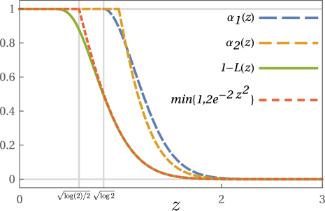
Figure 1: A comparison of functions $\alpha_{1}(z)$ and $\alpha_{2}(z)$ [defined in Propositions 2a and 2b] with $L(z)$ [used in Kolmogorov’s and Smirnov’s theorems] and $2e^{-2z^{2}}$ [used in the DKWM inequality, Wei and Dudley’s inequality, and in Proposition 1].

Figure 1 contrasts functions $\alpha_{1}(z)$ and $\alpha_{2}(z)$ [defined in Propositions 2a and 2b] with $L(z)$ [used in Kolmogorov’s and Smirnov’s theorems] and $2e^{-2z^{2}}$ [used in the DKWM and WD inequalities, and in Proposition 1].

Lemma 1.

KS-distances satisfy the inequality,

$$|d(F_{n},G_{m})-d(F,G)|\ \leq\ d(F_{n},F)+d(G_{m},G).$$ (13)

Proof.

As KS-distances are metric, we may use triangle inequalities to find an upper bound on $d(F_{n},G_{m})$ as $d(F_{n},G_{m})\leq d(F_{n},F)+d(F,G_{m})\leq d(F_{n},F)+d(G_{m},G)+d(F,G)$. A similar method applied to $d(F,G)$ results in the lower bound $d(F_{n},G_{m})\geq d(F,G)-d(F_{n},F)-d(G_{m},G)$. Together these bounds may be recast as Eq. (13).∎

Corollary 1.

From Lemma 1, it follows that for a given $z$, the statement $\big{|}d(F_{n},G_{m})-d(F,G)\big{|}>z$ implies the statement $d(F_{n},F)+d(G_{m},G)>z$. Hence,

$$\text{Prob}\Big{[}\big{|}d(F_{n},G_{m})-d(F,G)\big{|}>z\Big{]}\,\,\,\leq\,\,\,\text{Prob}\Big{[}d(F_{n},F)+d(G_{m},G)>z\Big{]}.$$ (14)

Notation 1.

In the following, we abbreviate $x_{F}:=d(F_{n},F)$ and $x_{G}:=d(G_{m},G)$, and denote the (potentially unknown) distributions satisfied by these as $\rho_{F}(x_{F})$ and $\rho_{G}(x_{G})$. It is also useful to define the function

$$\mu_{1}(n,x):=\begin{cases}8nxe^{-2nx^{2}}&\ \text{for}\ x\geq\sqrt{\frac{\log 2}{2n}}\\ 0&\mathrm{otherwise}\end{cases},$$ (15)

which we use to recast the DKWM inequality [Eq. (3)] in the form

$$\int_{0}^{z}\rho_{F}(x_{F})\mathrm{d}x_{F}\geq\int_{0}^{z}\mu_{1}(n,x_{F})\mathrm{d}x_{F}=\max\left(0,1-2e^{-2nz^{2}}\right).$$ (16)

Lemma 2.

For $z\leq 1$,

$$\mathrm{Prob}\left[x_{F}+x_{G}\leq z\right]\ \geq\ \int_{\omega_{1}}\mu_{1}(n,x_{F})\mu_{1}(m,x_{G})\mathrm{d}x_{F}\mathrm{d}x_{G},$$ (17)

where $\omega_{1}:=\{(x_{F},x_{G}):x_{F}+x_{g}\leq z\}$.

Proof.

As $x_{F}$ and $x_{G}$ are independent, the probability $\mathrm{Prob}\left[x_{F}+x_{G}\leq z\right]$ may be formally expressed as an integral of the combined probability distribution $\rho_{F}(x_{F})\rho_{G}(x_{G})$ over $\omega_{1}$. For $z\leq 1$, this is

$$\mathrm{Prob}\left[x_{F}+x_{G}\leq z\right]=\int_{0}^{z}\int_{0}^{z-x_{G}}\rho_{F}(x_{F})\rho_{G}(x_{G})\mathrm{d}x_{F}\mathrm{d}x_{G}\ \geq\ \int_{0}^{z}\int_{0}^{z-x_{G}}\mu_{1}(n,x_{F})\rho_{G}(x_{G})\mathrm{d}x_{F}\mathrm{d}x_{G},$$ (18)

where we have applied the DKWM inequality [Eq. (16)] to the $x_{F}$ integral. By switching the order of integration, we may once more apply the DKWM inequality, this time to the $x_{G}$ integral,

$$\int_{0}^{z}\int_{0}^{z-x_{F}}\mu_{1}(n,x_{F})\rho_{G}(x_{G})\mathrm{d}x_{G}\mathrm{d}x_{F}\ \geq\ \int_{0}^{z}\int_{0}^{z-x_{F}}\mu_{1}(n,x_{F})\mu_{1}(m,x_{G})\mathrm{d}x_{G}\mathrm{d}x_{F}.$$ (19)

∎

Proof of Proposition 2a.

The proof of Proposition 2a follows from Corollary 1 and Lemma 2, and evaluation of integral (17). We need only consider $z\leq 1$ as $|d(F_{n},G_{m})-d(F,G)|\leq 1$. The restriction to $z\geq\sqrt{\log(2)/2}(n^{-1/2}+m^{-1/2})$ is a consequence of the piecewise definition of $\mu_{1}$ in Eq. (15). ∎

We now turn to the proof of Proposition 2b, which follows a similar approach to that of Proposition 2a. Rather than relying on the inequality of Lemma 1, we make use of the following stronger inequality.

Lemma 3.

KS-distances $d(F_{n},G_{m})=\sup_{x}|F_{n}-G_{m}|$ and $d(F,G)=\sup_{x}|F-G|$ satisfy the inequality

$$\big{|}d(F_{n},G_{m})-d(F,G)\big{|}\ \leq\ \max\big{[}\sup_{x}(F_{n}-F)+\sup_{x}(G_{m}-G),\,\sup_{x}(F-F_{n})+\sup_{x}(G-G_{m})\big{]}.$$ (20)

Proof.

Consider the following procedure.

$$\left(F_{n}(x)-G_{m}(x)\right)-\left(F(x)-G(x)\right)=\left(F_{n}(x)-F(x)\right)+\left(G(x)-G_{m}(x)\right)$$ (21)

$$\left(F_{n}(x)-G_{m}(x)\right)-\left|F(x)-G(x)\right|\leq\left(F_{n}(x)-F(x)\right)+\left(G(x)-G_{m}(x)\right)$$ (22)

$$\left(F_{n}(x)-G_{m}(x)\right)-\sup_{x}\left|F-G\right|\leq\sup_{x}\left(F_{n}-F\right)+\sup_{x}\left(G-G_{m}\right)$$ (23)

$$\sup_{x}\left(F_{n}-G_{m}\right)-\sup_{x}\left|F-G\right|\leq\sup_{x}\left(F_{n}-F\right)+\sup_{x}\left(G-G_{m}\right)$$ (24)

Eq. (21) applies pointwise. The absolute value applied in Eq. (22) serves to introduce the inequality, and the sup’s introduced in Eq. (23) serve only to potentially loosen the inequality. Eq. (24) is reached as Eq. (23) is valid for all $x$. By making the replacements $F_{n}\leftrightarrow G_{m}$, $F\leftrightarrow G$ on the LHS and $F_{n}\leftrightarrow F$, $G_{m}\leftrightarrow G$ on the RHS of Eq. (21), an identical procedure may be followed to find

$$\sup_{x}\left(G_{m}-F_{n}\right)-\sup_{x}\left|G-F\right|\leq\sup_{x}\left(F-F_{n}\right)+\sup_{x}\left(G_{m}-G\right).$$ (25)

Then since $\sup_{x}\left|G-F\right|=\sup_{x}\left|F-G\right|$ and $\sup_{x}\left|F_{n}-G_{m}\right|=\max\left[\sup_{x}\left(F_{n}-G_{m}\right),\sup_{x}\left(G_{m}-F_{n}\right)\right]$, Eqs. (24) and (25) may be combined to give

$$\sup_{x}\left|F_{n}-G_{m}\right|-\sup_{x}\left|F-G\right|\ \leq\ \max\big{[}\sup_{x}\left(F_{n}-F\right)+\sup_{x}\left(G-G_{m}\right),\ \sup_{x}\left(F-F_{n}\right)+\sup_{x}\left(G_{m}-G\right)\big{]}.$$ (26)

Finally, this whole process may be repeated with the replacements $F_{n}\leftrightarrow F$ and $G_{m}\leftrightarrow G$, whereby the resulting equation may be combined with Eq. (26) to give Eq. (20).∎

Notation 2.

In the following we abbreviate as $x_{F}^{+}:=\sup_{x}(F_{n}-F)$, $x_{F}^{-}:=\sup_{x}(F-F_{n})$, $x_{G}^{+}:=\sup_{x}(G_{m}-G)$, and $x_{G}^{-}:=\sup_{x}(G-G_{m})$. Each of these satisfies the one-sided version of the DKWM inequality [see Thm. 1 in Massart (1990)], e.g. $\mathrm{Prob}(x_{F}^{+}>z)\leq\exp\left(-2nz^{2}\right)$ for all $z\geq\sqrt{\log 2/(2n)}$. (Strictly speaking, we also require that $z\geq 1.0841n^{-2/3}$, which we shall take as a given.) Similarly to our introduction of function $\mu_{1}$ in Notation 1, we define function $\mu_{2}(n,x):=4nx\exp\left(-2nx^{2}\right)$, which bounds the unknown distribution $\rho_{F^{+}}(x_{F}^{+})$ satisfied by $x_{F}^{+}$ in the sense that we may reexpress the DKWM inequality

$$\int_{0}^{z}\rho_{F^{+}}(x_{F}^{+})\mathrm{d}x_{F}^{+}\geq\int_{0}^{z}\mu_{2}(n,x_{F}^{+})\mathrm{d}x_{F}^{+}$$ (27)

for $z\geq\sqrt{\log 2/(2n)}$.

Corollary 2.

From Lemma 3, it follows that for a given $z$, the statement $\big{|}d(F_{n},G_{m})-d(F,G)\big{|}>z$ implies the statement $\max\big{(}x_{F}^{+}+x_{G}^{-},\,x_{F}^{-}+x_{G}^{+}\big{)}>z$. Hence,

$$\mathrm{Prob}\Big{[}\big{|}d(F_{n},G_{m})-d(F,G)\big{|}>z\Big{]}\ \leq\ \mathrm{Prob}\left[\max\big{(}x_{F}^{+}+x_{G}^{-},\,x_{F}^{-}+x_{G}^{+}\big{)}>z\right].$$ (28)

Lemma 4.

For $\sqrt{\log(2)/2}\left(n^{-1/2}+m^{-1/2}\right)\leq z\leq 1$,

$$\mathrm{Prob}\left[x_{F}^{+}+x_{G}^{-}\leq z\right]\ \geq\ \alpha_{3}:=\int_{\omega_{2}}\mu_{2}(n,x_{F}^{+})\mu_{2}(m,x_{G}^{-})\mathrm{d}x_{F}^{+}\mathrm{d}x_{G}^{-},$$ (29)

where $\omega_{2}:=\left\{(x_{F}^{+},x_{G}^{-}):x_{F}^{+}+x_{G}^{-}\leq z,\ x_{F}^{+}\leq z-\sqrt{\log 2/(2m)},\ x_{G}^{-}\leq z-\sqrt{\log 2/(2n)}\right\}$, and where we have defined $\alpha_{3}$ for later use. (It is also the case that $\mathrm{Prob}\left[x_{F}^{-}+x_{G}^{+}\leq z\right]\ \geq\ \alpha_{3}$.)

Proof.

For $z\leq 1$, $\mathrm{Prob}\left[x_{F}^{+}+x_{G}^{-}\leq z\right]=\int_{\omega_{3}}\rho_{F^{+}}(x_{F}^{+})\rho_{G^{-}}(x_{G}^{-})\mathrm{d}x_{F}^{+}\mathrm{d}x_{G}^{-}$, where $\omega_{3}:=\left\{(x_{F}^{+},x_{G}^{-}):x_{F}^{+}+x_{G}^{-}\leq z\right\}$. We may apply the one-sided DKWM inequality [Eq. (27)] to the $x_{F}^{+}$ integral provided its upper boundary exceeds or is equal to $\sqrt{\log 2/(2n)}$. We may ensure this by restricting to the integration domain to $\omega_{4}:=\left\{(x_{F}^{+},x_{G}^{-}):x_{F}^{+}+x_{G}^{-}\leq z,\ x_{G}^{-}\leq z-\sqrt{\log 2/(2n)}\right\}$, which only serves to loosen the resulting inequality, $\mathrm{Prob}\left[x_{F}^{+}+x_{G}^{-}\leq z\right]\geq\int_{\omega_{4}}\mu_{2}(x_{F}^{+})\rho_{G^{-}}(x_{G}^{-})\mathrm{d}x_{F}^{+}\mathrm{d}x_{G}^{-}$ . We may now switch the order of integration and apply the one-sided DKWM inequality to the $x_{G}^{-}$ integral provided its upper bound exceeds or is equal to $\sqrt{\log 2/(2m)}$. This results in the integration domain $\omega_{2}$ defined above. As $x_{F}^{+}\geq 0$ and $x_{G}^{-}\geq 0$, this domain requires $z\geq\sqrt{\log(2)/2}(n^{-1/2}+m^{-1/2})$.∎

Proof of Proposition 2b.

In light of Corollary 2, we look to place an upper bound on $\mathrm{Prob}\left[\max\big{(}x_{F}^{+}+x_{G}^{-},\,x_{F}^{-}+x_{G}^{+}\big{)}>z\right]=\mathrm{Prob}\left[x_{F}^{+}+x_{G}^{-}>z\ \bigcup\ x_{F}^{-}+x_{G}^{+}>z\right]=1-\mathrm{Prob}\left[x_{F}^{+}+x_{G}^{-}\leq z\ \bigcap\ x_{F}^{-}+x_{G}^{+}\leq z\right]$. Thus we may equivalently look for a lower bound on $\mathrm{Prob}\left[x_{F}^{+}+x_{G}^{-}\leq z\ \bigcap\ x_{F}^{-}+x_{G}^{+}\leq z\right]$. Due to Lemma 4, we have both $\mathrm{Prob}\left[x_{F}^{+}+x_{G}^{-}\leq z\right]\geq\alpha_{3}$ and $\mathrm{Prob}\left[x_{F}^{-}+x_{G}^{+}\leq z\right]\geq\alpha_{3}$. (We need only consider $z\leq 1$ as $|d(F_{n},G_{m})-d(F,G)|\leq 1$.) If $\alpha_{3}<1/2$, there is the potential for $\mathrm{Prob}\left[x_{F}^{+}+x_{G}^{-}\leq z\ \bigcap\ x_{F}^{-}+x_{G}^{+}\leq z\right]=0$. If however $\alpha_{3}>1/2$, the smallest the intersectional probability may be is $2\alpha_{3}-1$. Thus, $\mathrm{Prob}\left[x_{F}^{+}+x_{G}^{-}\leq z\ \bigcap\ x_{F}^{-}+x_{G}^{+}\leq z\right]\geq\max\left(0,\ 2\alpha_{3}-1\right)$, and so $\mathrm{Prob}\left[\max\big{(}x_{F}^{+}+x_{G}^{-},\,x_{F}^{-}+x_{G}^{+}\big{)}>z\right]\leq 1-\max\left(0,\ 2\alpha_{3}-1\right)=\min\left(1,2-2\alpha_{3}\right)$. Eq. (Proposition 2b) then follows from evaluation of $\alpha_{3}$ [Eq. (29)].∎

4 Conclusion

KS-distances that are calculated from data [$d(F_{n},G)$ in the one-sample case and $d(F_{n},G_{m})$ in the two-sample case] may be regarded as estimates of the underlying KS-distance, $d(F,G)$. The inequalities we have derived place probability bounds on the accuracy of these estimates. In the one-sample case, our Proposition 1 reduces to the DKWM-inequality when $d(F,G)=0$. When $d(F,G)=0$ in the two-sample case however, our Propositions 2a and 2b do not provide as tight a bound as that found by Wei and Dudley (2012). In addition to this, some preliminary numerical investigation suggests that the rate of convergence of $d(F_{n},G_{m})$ to $d(F,G)$ may quicken when $d(F,G)\neq 0$. For this reason, we speculate that it may be possible to find a tighter inequality in the two-sample case. Finally we note that our propositions in effect remove the $d(F,G)=0$ null hypothesis of standard Kolmogorov-Smirnov significance tests. To what extent this may inform such significance testing is an open question.

References

- Dvoretzky et al. (1956) A. Dvoretzky, J. Kiefer, and J. Wolfowitz. Asymptotic Minimax Character of the Sample Distribution Function and of the Classical Multinomial Estimator. Ann. Math. Stat., 27(3):642 – 669, 1956. doi:10.1214/aoms/1177728174.
- Feller (1948) W. Feller. On the Kolmogorov-Smirnov Limit Theorems for Empirical Distributions. Ann. Math. Stat., 19(2):177 – 189, 1948. doi:10.1214/aoms/1177730243.
- Kolmogorov (1933) A. Kolmogorov. Sulla determinazione empirica di una legge di distribuzione. G. Ist. Ital. Attuari, 4:83–91, 1933.
- Massart (1990) P. Massart. The Tight Constant in the Dvoretzky-Kiefer-Wolfowitz Inequality. Ann. Probab., 18(3):1269 – 1283, 1990. doi:10.1214/aop/1176990746.
- Smirnov (1939) N. Smirnov. On the estimation of the discrepancy between empirical curves of distribution for two independent samples. Moscow Univ. Math. Bull., 2, 1939.
- Wei and Dudley (2012) F. Wei and R. M. Dudley. Two-sample Dvoretzky–Kiefer–Wolfowitz inequalities. Stat. Probab. Lett., 82(3):636–644, 2012. doi:10.1016/j.spl.2011.11.012.