Explicit Local Time-Stepping for the Inhomogeneous Wave Equation with Optimal Convergence

Marcus J. Grote Department of Mathematics and Computer Science, University of Basel, Spiegelgasse 1, 4051 Basel, Switzerland, (marcus.grote@unibas.ch)    Simon R. J. Michel Mathematisches Institut, Universität Bern, Sidlerstrasse 5, 3012 Bern, Switzerland, (simon.michel@unibe.ch)    Stefan A. Sauter Institute for Mathematics, University of Zurich, Winterthurerstrasse 190, 8057 Zurich, Switzerland, (stas@math.uzh.ch)
Abstract

Adaptivity and local mesh refinement are crucial for the efficient numerical simulation of wave phenomena in complex geometry. Local mesh refinement, however, can impose a tiny time-step across the entire computational domain when using explicit time integration. By taking smaller time-steps yet only inside locally refined regions, local time-stepping methods overcome the stringent CFL stability restriction imposed on the global time-step by a small fraction of the elements without sacrificing explicitness. In [21], a leapfrog based local time-stepping method was proposed for the inhomogeneous wave equation, which applies standard leapfrog time-marching with a smaller time-step inside the refined region. Here, to remove potential instability at certain time-steps, a stabilized version is proposed which leads to optimal L2superscript𝐿2L^{2}-error estimates under a CFL condition independent of the coarse-to-fine mesh ratio. Moreover, a weighted transition is introduced to restore optimal H1superscript𝐻1H^{1}-convergence when the source is nonzero across the coarse-to-fine mesh interface. Numerical experiments corroborate the theoretical error estimates and illustrate the usefulness of these improvements.

1 Introduction

For the simulation of wave phenomena, finite element methods, be it conforming or discontinuous, easily accommodate complex geometry or material interfaces. Local mesh refinement, however, seriously hampers the efficiency of explicit time integrators, such as the popular leapfrog (LF) method, when a small fraction of elements impose a tiny time-step for stability across the entire mesh. By taking smaller time-steps, but only inside those refined regions, while taking larger time-steps elsewhere, local time-stepping methods (LTS) permit to overcome that overly stringent CFL stability constraint on the global time-step without sacrificing the explicitness or parallel efficiency of explicit time integrators.

Following the classical IMEX (implicit-explicit) approach, first locally implicit methods that combine the (explicit) second-order LF (or Størmer-Verlet) method in the coarse part with the (implicit) Crank-Nicolson method in the fine part of the mesh were proposed and further analyzed in [30, 16, 33, 12, 23, 24]. In [5], fourth-order energy-preserving IMEX schemes were derived for the wave equation, when the computational domain is divided into a coarse and fine region using Lagrange multipliers along the interface.

Even earlier, an explicit local time-stepping (LTS) method was proposed for the wave equation, which also employs the explicit LF method in the fine part of the mesh, yet with a smaller step-size [9, 11]; error estimates were derived in [10, 26] in the one-dimensional case. Stability of this second-order method, however, is guaranteed by enforcing energy conservation which requires at every time-step the solution of a linear system for the shared unknowns at the coarse/fine intersection; hence, the overall scheme is not fully explicit.

Fully explicit second-order LTS methods based on Størmer-Verlet in time and DG discretizations in space were proposed for Maxwell’s equations in [30, 29]. Starting from the popular LF method, fully explicit local time-stepping methods of arbitrary order were proposed for the homogeneous wave equation in [13] and for the inhomogeneous wave equation with nonzero forcing in [21]. Inside the locally refined region, they apply standard leapfrog time-marching with a smaller time-step, which also implies evaluating the inhomogeneous right-hand side at all intermediate times. Hence, when combined with a mass-lumped conforming [8, 7] or discontinuous Galerkin FE discretization [22] in space, the resulting LF-LTS method is truly explicit, inherently parallel and also conserves a discrete energy in the absence of forcing; it was successfully applied to 3D seismic wave propagation [28]. A multilevel version was later proposed [14] and achieved high parallel efficiency [31].

In [19], optimal L2superscript𝐿2L^{2}-error estimates for the LF-LTS method from [13] were derived for H1superscript𝐻1H^{1}-conforming FEM discretizations (with mass-lumping), though under a CFL condition where the global time-step ΔtΔ𝑡\Delta t in fact depended on the smallest elements in the mesh. For the convergence analysis, the inner loop over the p𝑝p local LF steps of size Δt/pΔ𝑡𝑝\Delta t/p was rewritten in terms of a single global time-step ΔtΔ𝑡\Delta t, which involves Chebyshev polynomials of the first kind. In general one cannot improve upon the stability constraint on ΔtΔ𝑡\Delta t, as the LF-LTS method may become unstable at certain values of ΔtΔ𝑡\Delta t.

By replacing those Chebyshev polynomials by “damped” Chebyshev polynomials with damping parameter ν>0𝜈0\nu>0, which slightly modifies the LF-LTS scheme inside the refined region, a stabilized LF-LTS(ν𝜈\nu) version was proposed in [20] for the homogeneous wave equation, and also independently in [2], which led to optimal L2superscript𝐿2L^{2}-error estimates yet under a CFL condition independent of the coarse-to-fine aspect ratio. The same damped Chebyshev polynomials were also previously used to stabilize leapfrog-Chebyshev (LFC, discrete Gautschi-type) methods [18, 4], where the “non-stiff” (or slowly varying), possibly nonlinear source term is evaluated only at every global time-step throughout the entire computational domain. In fact, the error analysis for semilinear ODE’s in [2] and for DG discretizations of linear wave equations in [3] both apply to the inhomogeneous case, too, when the source is evaluated only once during each global time-step, akin to the approach in [4].

Main contributions. The leapfrog based local time-stepping (LF-LTS) method introduced in [21] for the inhomogeneous wave equation can become unstable for certain time-steps. To remove those potential instabilities, we propose a stabilized version which leads to optimal L2superscript𝐿2L^{2}-error estimates under a CFL condition independent of the coarse-to-fine mesh ratio. Thus we effectively introduce stabilization into the original method from [21], which, in contrast to the “split-LFC” method from [3], corresponds to standard LF time-marching, yet with a smaller time-step, inside the refined region. Generalizing the proof of L2superscript𝐿2L^{2}-convergence for the homogeneous wave equation [20] to the inhomogeneous case is not straightforward due to the source evaluations at all intermediate local time-steps. In fact it requires the development of new analytical techniques involving Chebyshev polynomials of the second kind to rewrite and analyze the effect of those local time-steps and thus finally prove the stability and optimal consistency order of the method.

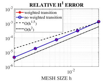
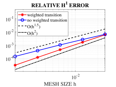
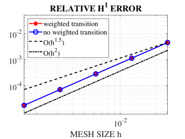
In [6] it was shown that the expected optimal H1superscript𝐻1H^{1}-convergence rate of the LF-LTS method [21] for the inhomogeneous wave equation is reduced by h1/2superscript12h^{1/2} when the source is nonzero across the coarse-to-fine mesh interface. To overcome this difficulty and thereby restore optimal H1superscript𝐻1H^{1}-convergence, we introduce a new weighted transition which relies on a discrete mesh-based distance function.

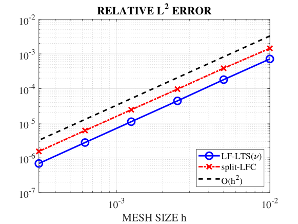
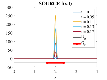
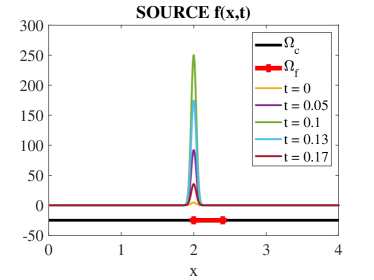
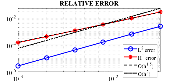
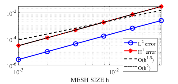
Outline. The rest of our article is structured as follows. In Section 2, we first recall the H1superscript𝐻1H^{1}-conforming Galerkin formulation of the inhomogeneous wave equation together with needed notation as the mesh is split into a coarse and a locally refined part. In Section 2.3, this leads to the stabilized LF-LTS(ν)𝜈(\nu) algorithm for the inhomogenous wave equation, which also evaluates the source term inside the locally refined region at all intermediate time-steps. In Section 3, we prove optimal L2superscript𝐿2L^{2}-convergence rates under a CFL condition independent of the fine-to-coarse mesh ratio. To accomodate for the intermediate source evaluations, our error analysis requires both Chebyshev polynomials of the first and the second kind. Still our analysis also includes the somewhat simpler situation when the source is evaluated at global time-steps only as in [3]. To achieve optimal H1superscript𝐻1H^{1}-convergence regardless of the source, we introduce in Section 4 the new weighted transition which relies on a discrete mesh-based distance function. In Section 5, we present numerical experiments which illustrate the optimal L2superscript𝐿2L^{2}-convergence rates expected from theory. In doing so, we also compare the LF-LTS method with the alternative “split-LFC” approach from [3], where the source inside the locally refined region is only evaluated once at each global time-step. While both LTS methods, either with or without intermediate local source evaluations, are second-order convergent in ΔtΔ𝑡\Delta t, our approach is more accurate (but also slightly more expensive) than the LTS method from [3] when the source strongly varies locally. Finally, we revisit the original example from [6] and show that the new weighted transition restores the expected optimal H1superscript𝐻1H^{1}-convergence rate even when the source is nonzero across the coarse-to-fine mesh interface.

2 Stabilized LF-LTS Method

In Sections 2.1 and 2.2, we adopt and recall the setting for finite element spaces as in [20].

2.1 The Wave Equation

Let ΩdΩsuperscript𝑑\Omega\subset\mathbb{R}^{d} be a bounded Lipschitz domain with boundary Γ=ΩΓΩ\Gamma=\partial\Omega. For 1q1𝑞1\leq q\leq\infty, let Lq(Ω)superscript𝐿𝑞ΩL^{q}\left(\Omega\right) be the standard Lebesgue space with norm Lq(Ω)\left\|\cdot\right\|_{L^{q}\left(\Omega\right)}. For q=2𝑞2q=2, the scalar product in L2(Ω)superscript𝐿2ΩL^{2}\left(\Omega\right) is denoted by (,)\left(\cdot,\cdot\right) and the norm by :=L2(Ω)\left\|\cdot\right\|:=\left\|\cdot\right\|_{L^{2}\left(\Omega\right)}. For k0𝑘subscript0k\in\mathbb{N}_{0} and 1q1𝑞1\leq q\leq\infty, let Wk,q(Ω)superscript𝑊𝑘𝑞ΩW^{k,q}\left(\Omega\right) denote the classical Sobolev spaces equipped with the norm Wk,q(Ω)\left\|\cdot\right\|_{W^{k,q}\left(\Omega\right)}. For q=2𝑞2q=2, these spaces are Hilbert spaces and denoted by Hk(Ω):=Wk,2(Ω)assignsuperscript𝐻𝑘Ωsuperscript𝑊𝑘2ΩH^{k}\left(\Omega\right):=W^{k,2}\left(\Omega\right) with scalar product (,)Hk(Ω)subscriptsuperscript𝐻𝑘Ω\left(\cdot,\cdot\right)_{H^{k}\left(\Omega\right)} and norm Hk(Ω):=(,)Hk(Ω)1/2=Wk,2(Ω)\left\|\cdot\right\|_{H^{k}\left(\Omega\right)}:=\left(\cdot,\cdot\right)_{H^{k}\left(\Omega\right)}^{1/2}=\left\|\cdot\right\|_{W^{k,2}\left(\Omega\right)}.

We assume that the boundary is split into a Dirichlet and a Neumann part: Γ=ΓDΓNΓsubscriptΓ𝐷subscriptΓ𝑁\Gamma=\Gamma_{D}\cup\Gamma_{N}, ΓDΓN=subscriptΓ𝐷subscriptΓ𝑁\Gamma_{D}\cap\Gamma_{N}=\emptyset with the convention that ΓDsubscriptΓ𝐷\Gamma_{D} is (relatively) closed and has positive surface measure. On ΓDsubscriptΓ𝐷\Gamma_{D} homogeneous Dirichlet boundary conditions are imposed and Neumann boundary conditions on ΓNsubscriptΓ𝑁\Gamma_{N}. The space of Sobolev functions in H1(Ω)superscript𝐻1ΩH^{1}\left(\Omega\right) which vanish on the Dirichlet part of the boundary ΩΩ\partial\Omega is denoted by HD1(Ω):={wH1(Ω):w|ΓD=0}assignsuperscriptsubscript𝐻𝐷1Ωconditional-set𝑤superscript𝐻1Ωevaluated-at𝑤subscriptΓ𝐷0H_{D}^{1}\left(\Omega\right):=\left\{w\in H^{1}\left(\Omega\right):\left.w\right|_{\Gamma_{D}}=0\right\}. For ΓD=ΓsubscriptΓ𝐷Γ\Gamma_{D}=\Gamma, we use the shorthand H01(Ω)superscriptsubscript𝐻01ΩH_{0}^{1}\left(\Omega\right). Throughout this paper we restrict ourselves to function spaces over the field of real numbers.

Let VH1(Ω)𝑉superscript𝐻1ΩV\subset H^{1}\left(\Omega\right) denote a closed subspace of H1(Ω)superscript𝐻1ΩH^{1}\left(\Omega\right), such as V=H1(Ω)𝑉superscript𝐻1ΩV=H^{1}\left(\Omega\right) or V=H01(Ω)𝑉superscriptsubscript𝐻01ΩV=H_{0}^{1}\left(\Omega\right), and a:V×V:𝑎𝑉𝑉a:V\times V\rightarrow\mathbb{R} denote a bilinear form, which is symmetric, continuous, and coercive:

a(u,v)=a(v,u)u,vVformulae-sequence𝑎𝑢𝑣𝑎𝑣𝑢for-all𝑢𝑣𝑉a\left(u,v\right)=a\left(v,u\right)\qquad\forall u,v\in V (2.1a)

and

|a(u,v)|CcontuH1(Ω)vH1(Ω)u,vVformulae-sequence𝑎𝑢𝑣subscript𝐶contsubscriptnorm𝑢superscript𝐻1Ωsubscriptnorm𝑣superscript𝐻1Ωfor-all𝑢𝑣𝑉\left|a\left(u,v\right)\right|\leq C_{\operatorname*{cont}}\left\|u\right\|_{H^{1}\left(\Omega\right)}\left\|v\right\|_{H^{1}\left(\Omega\right)}\qquad\forall u,v\in V (2.1b)

and

a(u,u)ccoeruH1(Ω)2uV.formulae-sequence𝑎𝑢𝑢subscript𝑐coersuperscriptsubscriptnorm𝑢superscript𝐻1Ω2for-all𝑢𝑉a\left(u,u\right)\geq c_{\operatorname*{coer}}\left\|u\right\|_{H^{1}\left(\Omega\right)}^{2}\qquad\forall u\in V. (2.1c)

For given u0V,v0L2(Ω)formulae-sequencesubscript𝑢0𝑉subscript𝑣0superscript𝐿2Ωu_{0}\in V,v_{0}\in L^{2}\left(\Omega\right) and F:[0,T]V:𝐹0𝑇superscript𝑉F:\left[0,T\right]\rightarrow V^{\prime}, we consider the wave equation: Find u:[0,T]V:𝑢0𝑇𝑉u:\left[0,T\right]\rightarrow V such that

(u¨,w)+a(u,w)=F(w)wV,t>0formulae-sequence¨𝑢𝑤𝑎𝑢𝑤𝐹𝑤formulae-sequencefor-all𝑤𝑉𝑡0\left(\ddot{u},w\right)+a\left(u,w\right)=F\left(w\right)\quad\forall w\in V,t>0 (2.2)

with initial conditions

u(0)=u0and u˙(0)=v0.formulae-sequence𝑢0subscript𝑢0and ˙𝑢0subscript𝑣0u\left(0\right)=u_{0}\quad\text{and\quad}\dot{u}\left(0\right)=v_{0}. (2.3)

It is well known that (2.2)–(2.3) is well-posed for sufficiently regular u0subscript𝑢0u_{0}, v0subscript𝑣0v_{0} and F𝐹F [27]. In fact, the weak solution u𝑢u can be shown to be continuous in time, that is, uC0(0,T;V),u˙C0(0,T;L2(Ω))formulae-sequence𝑢superscript𝐶00𝑇𝑉˙𝑢superscript𝐶00𝑇superscript𝐿2Ωu\in C^{0}(0,T;V),\dot{u}\in C^{0}(0,T;L^{2}\left(\Omega\right)) – see [27, Chapter III, Theorems 8.1 and 8.2] for details – which implies that the initial conditions (2.3) are well defined. Moreover, we always assume that there exists a function f:[0,T]L2(Ω):𝑓0𝑇superscript𝐿2Ωf:\left[0,T\right]\rightarrow L^{2}\left(\Omega\right) such that

F(t)(w)=(f(t),w)wVt[0,T].formulae-sequence𝐹𝑡𝑤𝑓𝑡𝑤formulae-sequencefor-all𝑤𝑉for-all𝑡0𝑇F\left(t\right)\left(w\right)=\left(f\left(t\right),w\right)\qquad\forall w\in V\quad\forall t\in\left[0,T\right].

For the stability and convergence analysis we will impose further smoothness assumptions on f𝑓f.

Example 1

The classical second-order wave equation in strong form is given by

t2u(c2u)=fin Ω×(0,T),u=0on ΓD×(0,T),uν=0on ΓN×(0,T),u|t=0=u0in Ω,ut|t=0=v0in Ω,formulae-sequencesuperscriptsubscript𝑡2𝑢superscript𝑐2𝑢𝑓in Ω0𝑇formulae-sequence𝑢0on subscriptΓ𝐷0𝑇formulae-sequence𝑢𝜈0on subscriptΓ𝑁0𝑇formulae-sequenceevaluated-at𝑢𝑡0subscript𝑢0in Ωevaluated-atsubscript𝑢𝑡𝑡0subscript𝑣0in Ω\begin{split}\partial_{t}^{2}u-\nabla\cdot(c^{2}\nabla u)&=f\qquad\;\,\mbox{in }\Omega\times(0,T),\\ u&=0\qquad\;\,\mbox{on }\Gamma_{D}\times(0,T),\\ \frac{\partial u}{\partial\nu}&=0\qquad\;\,\mbox{on }\Gamma_{N}\times(0,T),\\ u|_{t=0}&=u_{0}\qquad\mbox{in }\Omega,\\ u_{t}|_{t=0}&=v_{0}\qquad\mbox{in }\Omega,\\ &\end{split} (2.4)

where the velocity field c(x)𝑐𝑥c(x) satisfies 0<cminc(x)cmax0subscript𝑐𝑐𝑥subscript𝑐0<c_{\min}\leq c(x)\leq c_{\max}. In this case, we have V:=HD1(Ω):={wH1(Ω):w|ΓD=0}assign𝑉superscriptsubscript𝐻𝐷1Ωassignconditional-set𝑤superscript𝐻1Ωevaluated-at𝑤subscriptΓ𝐷0V:=H_{D}^{1}\left(\Omega\right):=\left\{w\in H^{1}\left(\Omega\right):\left.w\right|_{\Gamma_{D}}=0\right\}; the bilinear form is given by a(u,v):=(c2u,u)assign𝑎𝑢𝑣superscript𝑐2𝑢𝑢a\left(u,v\right):=\left(c^{2}\nabla u,\nabla u\right) and the right-hand side by F(w)=(f,w)𝐹𝑤𝑓𝑤F\left(w\right)=\left(f,w\right) for all wV𝑤𝑉w\in V.

2.2 Galerkin Finite Element Spatial Discretization

We begin by briefly introducing our notation for hp𝑝hp finite element spaces. Let 𝒯𝒯\mathcal{T} be a simplicial finite element mesh for ΩΩ\Omega which is conforming in the sense that there are no hanging nodes. The local and global mesh width is

hτ:=diamτ,h:=maxτ𝒯hτ.formulae-sequenceassignsubscript𝜏diam𝜏assignsubscript𝜏𝒯subscript𝜏h_{\tau}:=\operatorname*{diam}\tau,\quad h:=\max_{\tau\in\mathcal{T}}h_{\tau}.

As a convention the triangles in 𝒯𝒯\mathcal{T} are closed sets. Without loss of generality, we may assume that there is fixed h0>0subscript00h_{0}>0 such that

hh0.subscript0h\leq h_{0}. (2.5)

The finite element space of continuous, piecewise polynomials of degree m1𝑚1m\geq 1 is denoted by

S𝒯m:={uC0(Ω)τ𝒯u|τm},assignsuperscriptsubscript𝑆𝒯𝑚conditional-set𝑢superscript𝐶0Ωformulae-sequencefor-all𝜏𝒯evaluated-at𝑢𝜏subscript𝑚S_{\mathcal{T}}^{m}:=\left\{u\in C^{0}\left(\Omega\right)\mid\forall\tau\in\mathcal{T}\quad\left.u\right|_{\tau}\in\mathbb{P}_{m}\right\},

where msubscript𝑚\mathbb{P}_{m} is the space of polynomials of maximal total degree m𝑚m. The standard local nodal basis is denoted by bm,zsubscript𝑏𝑚𝑧b_{m,z}, zΣ𝒯m𝑧superscriptsubscriptΣ𝒯𝑚z\in\Sigma_{\mathcal{T}}^{m}, where Σ𝒯msuperscriptsubscriptΣ𝒯𝑚\Sigma_{\mathcal{T}}^{m} is the full set of nodal points of order m𝑚m. The finite element space with incorporated Dirichlet boundary conditions is given by S:=S𝒯mVassign𝑆superscriptsubscript𝑆𝒯𝑚𝑉S:=S_{\mathcal{T}}^{m}\cap V. The set of nodal points for S𝑆S is the subset Σ:={zΣ𝒯mzΓD}assignΣconditional-set𝑧superscriptsubscriptΣ𝒯𝑚𝑧subscriptΓD\Sigma:=\left\{z\in\Sigma_{\mathcal{T}}^{m}\mid z\in\Gamma_{\operatorname*{D}}\right\} and the basis in S𝑆S is denoted by bz:=bm,zassignsubscript𝑏𝑧subscript𝑏𝑚𝑧b_{z}:=b_{m,z}, zΣ𝑧Σz\in\Sigma. Furthermore, we use the notion of a mass-lumped scalar product

(u,v)𝒯:=zΣdzu(z)v(z),u,vSformulae-sequenceassignsubscript𝑢𝑣𝒯subscript𝑧Σsubscript𝑑𝑧𝑢𝑧𝑣𝑧for-all𝑢𝑣𝑆\left(u,v\right)_{\mathcal{T}}:=\sum_{z\in\Sigma}d_{z}u\left(z\right)v\left(z\right),\quad\forall u,v\in S

for certain coefficients dz>0subscript𝑑𝑧0d_{z}>0 and induced norm 𝒯:=(,)𝒯1/2\|\cdot\|_{\mathcal{T}}:=\left(\cdot,\cdot\right)_{\mathcal{T}}^{1/2} which is assumed to be equivalent to the L2(Ω)superscript𝐿2ΩL^{2}\left(\Omega\right)-norm: there exists a constant Ceq>0subscript𝐶eq0C_{\operatorname*{eq}}>0 such that

Ceq1u𝒯uCequ𝒯uS.formulae-sequencesuperscriptsubscript𝐶eq1subscriptnorm𝑢𝒯norm𝑢subscript𝐶eqsubscriptnorm𝑢𝒯for-all𝑢𝑆.C_{\operatorname*{eq}}^{-1}\left\|u\right\|_{\mathcal{T}}\leq\left\|u\right\|\leq C_{\operatorname*{eq}}\left\|u\right\|_{\mathcal{T}}\quad\forall u\in S\text{.} (2.6)

For more details we refer, e.g., to [20, Definition 2.3].

We also associate to the discrete bilinear form the linear operator AS:SS:superscript𝐴𝑆𝑆𝑆A^{S}:S\rightarrow S defined by

(ASu,v)𝒯=a(u,v)u,vSformulae-sequencesubscriptsuperscript𝐴𝑆𝑢𝑣𝒯𝑎𝑢𝑣for-all𝑢𝑣𝑆\left(A^{S}u,v\right)_{\mathcal{T}}=a\left(u,v\right)\qquad\forall u,v\in S (2.7)

and introduce the discrete right-hand side function fS:[0,T]S:subscript𝑓𝑆0𝑇𝑆f_{S}:[0,T]\rightarrow S defined by

(fS(t),v)𝒯=F(t)(v)vSt[0,T].formulae-sequencesubscriptsubscript𝑓𝑆𝑡𝑣𝒯𝐹𝑡𝑣formulae-sequencefor-all𝑣𝑆for-all𝑡0𝑇\left(f_{S}(t),v\right)_{\mathcal{T}}=F(t)(v)\qquad\forall\,v\in S\quad\forall\,t\in[0,T].

With the definitions and notation at hand, the semi-discrete wave equation (with mass-lumping) is given by: find uS:[0,T]S:subscript𝑢𝑆0𝑇𝑆u_{S}:\left[0,T\right]\rightarrow S such that

(u¨S,v)𝒯+a(uS,v)=(fS(t),v)𝒯vS,t>0formulae-sequencesubscriptsubscript¨𝑢𝑆𝑣𝒯𝑎subscript𝑢𝑆𝑣subscriptsubscript𝑓𝑆𝑡𝑣𝒯formulae-sequencefor-all𝑣𝑆𝑡0\left(\ddot{u}_{S},v\right)_{\mathcal{T}}+a\left(u_{S},v\right)=\left(f_{S}(t),v\right)_{\mathcal{T}}\quad\forall v\in S,t>0 (2.8a)

with initial conditions

uS(0)=rSu0and u˙S(0)=rSv0,formulae-sequencesubscript𝑢𝑆0subscript𝑟𝑆subscript𝑢0and subscript˙𝑢𝑆0subscript𝑟𝑆subscript𝑣0u_{S}\left(0\right)=r_{S}u_{0}\quad\text{and\quad}\dot{u}_{S}\left(0\right)=r_{S}v_{0}, (2.8b)

where rSu0subscript𝑟𝑆subscript𝑢0r_{S}u_{0} is a finite element approximation of u0subscript𝑢0u_{0} (see, e.g., [20, (2.8)]).

As in [20], we consider finite element meshes 𝒯𝒯\mathcal{T} which consist of a quasi-uniform part 𝒯c𝒯subscript𝒯c𝒯\mathcal{T}_{\operatorname*{c}}\subset\mathcal{T} and allow for local refinements so that 𝒯f:=𝒯\𝒯cassignsubscript𝒯f\𝒯subscript𝒯c\mathcal{T}_{\operatorname*{f}}:=\mathcal{T}\backslash\mathcal{T}_{\operatorname*{c}} might contain much smaller triangles than 𝒯csubscript𝒯c\mathcal{T}_{\operatorname{c}}. In this way, we assume that the mesh size of 𝒯csubscript𝒯c\mathcal{T}_{\operatorname{c}} satisfies hc=hsubscriptch_{\operatorname{c}}=h. Similarly, we define coarse and locally refined regions of the domain111By int(M)int𝑀\operatorname*{int}\left(M\right) we denote the open interior of a subset Md𝑀superscript𝑑M\subset\mathbb{R}^{d}. as

Ωc:=int(τ𝒯cτ),Ωf:=int(τ𝒯fτ),Ωf+1:=int(τ𝒯τΩf¯τ).formulae-sequenceassignsubscriptΩcintsubscript𝜏subscript𝒯c𝜏formulae-sequenceassignsubscriptΩfintsubscript𝜏subscript𝒯f𝜏assignsuperscriptsubscriptΩf1intsubscript𝜏𝒯𝜏¯subscriptΩf𝜏\Omega_{\operatorname*{c}}:=\operatorname*{int}\left({\textstyle\bigcup\nolimits_{\tau\in\mathcal{T}_{\operatorname*{c}}}}\tau\right),\quad\Omega_{\operatorname*{f}}:=\operatorname*{int}\left({\textstyle\bigcup\nolimits_{\tau\in\mathcal{T}_{\operatorname*{f}}}}\tau\right),\quad\Omega_{\operatorname*{f}}^{+1}:=\operatorname*{int}\left({\textstyle\bigcup\nolimits_{\begin{subarray}{c}\tau\in\mathcal{T}\\ \tau\cap\overline{\Omega_{\operatorname*{f}}}\neq\emptyset\end{subarray}}}\,\tau\right). (2.9)

Hence, Ωf+1superscriptsubscriptΩf1\Omega_{\operatorname*{f}}^{+1} contains ΩfsubscriptΩf\Omega_{\operatorname*{f}} and all elements directly adjacent to it. We note that ΩfsubscriptΩf\Omega_{\operatorname*{f}} and ΩcsubscriptΩc\Omega_{\operatorname*{c}} are disjoint, while their union covers all of ΩΩ\Omega except for the coarse/fine interface, and that ΩcΩf+1=ΩsubscriptΩcsuperscriptsubscriptΩf1Ω\Omega_{\operatorname*{c}}\cup\Omega_{\operatorname*{f}}^{+1}=\Omega since the interface between ΩfsubscriptΩf\Omega_{\operatorname*{f}} and ΩcsubscriptΩc\Omega_{\operatorname*{c}} is contained in Ωf+1superscriptsubscriptΩf1\Omega_{\operatorname*{f}}^{+1}.

We also split the degrees of freedom associated with the fine or coarse parts of the mesh, respectively, as

Σf:=ΣΩf¯and Σc:=Σ\Σf,formulae-sequenceassignsubscriptΣfΣ¯subscriptΩfassignand subscriptΣc\ΣsubscriptΣf\Sigma_{\operatorname*{f}}:=\Sigma\cap\overline{\Omega_{\operatorname*{f}}}\quad\text{and\quad}\Sigma_{\operatorname*{c}}:=\Sigma\backslash\Sigma_{\operatorname*{f}},

and introduce the corresponding FE subspaces

Sc:=span{bz:zΣc}andSf:=span{bz:zΣf},formulae-sequenceassignsubscript𝑆cspan:subscript𝑏𝑧𝑧subscriptΣcandassignsubscript𝑆fspan:subscript𝑏𝑧𝑧subscriptΣfS_{\operatorname*{c}}:=\operatorname{span}\left\{b_{z}:z\in\Sigma_{\operatorname*{c}}\right\}\quad\mbox{and}\quad S_{\operatorname*{f}}:=\operatorname{span}\left\{b_{z}:z\in\Sigma_{\operatorname*{f}}\right\},

which gives rise to a direct sum decomposition: for every uS𝑢𝑆u\in S there exist unique functions ucScsubscript𝑢csubscript𝑆cu_{\operatorname*{c}}\in S_{\operatorname*{c}} and ufSfsubscript𝑢fsubscript𝑆fu_{\operatorname*{f}}\in S_{\operatorname*{f}} such that

u=uc+uf.𝑢subscript𝑢csubscript𝑢fu=u_{\operatorname*{c}}+u_{\operatorname*{f}}. (2.10)

Hence, we can define the projections ΠcS:SSc:superscriptsubscriptΠc𝑆𝑆subscript𝑆c\Pi_{\operatorname*{c}}^{S}:S\rightarrow S_{\operatorname*{c}} and ΠfS:SSf:superscriptsubscriptΠf𝑆𝑆subscript𝑆f\Pi_{\operatorname*{f}}^{S}:S\rightarrow S_{\operatorname*{f}} by

ΠcSu:=ucandΠfSu:=uf.formulae-sequenceassignsuperscriptsubscriptΠc𝑆𝑢subscript𝑢candassignsuperscriptsubscriptΠf𝑆𝑢subscript𝑢f\Pi_{\operatorname*{c}}^{S}u:=u_{\operatorname*{c}}\quad\text{and}\quad\Pi_{\operatorname*{f}}^{S}u:=u_{\operatorname*{f}}. (2.11)

In fact, the decomposition (2.10) is orthogonal with respect to the (,)𝒯subscript𝒯\left(\cdot,\cdot\right)_{\mathcal{T}} scalar product [20, Lemma 3.2], which is essential to prove sharp bounds for the eigenvalues of our discrete bilinearform [20, Theorem 3.7].

2.3 Stabilized LF-LTS(ν𝜈\nu) Algorithm

The original leapfrog (LF) based local time-stepping (LF-LTS(0)0(0)) methods for the numerical solution of the second-order wave equations (2.2) were proposed for homogeneous right-hand sides in [13] and for inhomogeneous right-hand sides in [21]. Optimal convergence rates for the LF-LTS(0)0(0) method from [13] with p𝑝p local time steps were derived for a conforming FEM discretization, albeit under a CFL condition where ΔtΔ𝑡\Delta t in fact depends on the smallest elements in the mesh [19]. To prove optimal L2superscript𝐿2L^{2} convergence rates under a CFL condition independent of p𝑝p, a stabilized algorithm LF-LTS(ν)𝜈(\nu) was introduced recently in [20], and also independently in [2]. Here, ν0𝜈0\nu\geq 0 denotes a small stabilization parameter; typically, we set ν=0.01𝜈0.01\nu=0.01. Stability and convergence for homogeneous right-hand sides were derived in [20] for a CFL condition independent of the coarse/fine mesh ratio.

We shall now extend this stabilized LF-LTS(ν)𝜈(\nu) method to inhomogeneous right-hand sides so that for ν=0𝜈0\nu=0 the method coincides with the original LF-LTS(0)0(0) method [21, Sect. 4.1] for the inhomogeneous wave equation. To do so, let the (global) time-step Δt=T/NΔ𝑡𝑇𝑁\Delta t=T/N and uS(n)superscriptsubscript𝑢𝑆𝑛u_{S}^{\left(n\right)} denote the FE approximation at time tn=nΔtsubscript𝑡𝑛𝑛Δ𝑡t_{n}=n\Delta t. Given the numerical solution at times tn1subscript𝑡𝑛1t_{n-1} and tnsubscript𝑡𝑛t_{n}, the LF-LTS method then computes the numerical solution of (2.8) at tn+1subscript𝑡𝑛1t_{n+1} by using a smaller time-step Δτ=Δt/pΔ𝜏Δ𝑡𝑝\Delta\tau=\Delta t/p inside the regions of local refinement; here, p2𝑝2p\geq 2 denotes the “coarse” to “fine” time-step ratio.

Inside the fine region, the source f𝑓f is also evaluated over the time interval [tnΔt,tn+Δt]subscript𝑡𝑛Δ𝑡subscript𝑡𝑛Δ𝑡[t_{n}-\Delta t,t_{n}+\Delta t] at the intermediate times tn+k/p=(n+k/p)Δtsubscript𝑡𝑛𝑘𝑝𝑛𝑘𝑝Δ𝑡t_{n+k/p}=\left(n+k/p\right)\Delta t and we let

fS,k(n):=fS(tn+kpΔt),pkp.formulae-sequenceassignsuperscriptsubscript𝑓𝑆𝑘𝑛subscript𝑓𝑆subscript𝑡𝑛𝑘𝑝Δ𝑡𝑝𝑘𝑝f_{S,k}^{(n)}:=f_{S}\left(t_{n}+\frac{k}{p}\Delta t\right),\quad-p\leq k\leq p.

The cost of those extra evaluations inside the locally refined region is typically negligible compared to the overall solution process. Still, a locally strongly varying source typically calls for such a a higher sampling of the right-hand side – see Section 5.1.

Given the fixed stabilization parameter 0ν1/20𝜈120\leq\nu\leq 1/2, we now define the following constants determined by stabilized versions [25] of Chebyshev polynomials of the first and second kind [32], denoted by Tnsubscript𝑇𝑛T_{n} and Unsubscript𝑈𝑛U_{n}, respectively:

δp,ν:=1+νp2,ωp,ν:=2Tp(δp,ν)Tp(δp,ν),formulae-sequenceassignsubscript𝛿𝑝𝜈1𝜈superscript𝑝2assignsubscript𝜔𝑝𝜈2superscriptsubscript𝑇𝑝subscript𝛿𝑝𝜈subscript𝑇𝑝subscript𝛿𝑝𝜈\delta_{p,\nu}:=1+\frac{\nu}{p^{2}},\qquad\omega_{p,\nu}:=2\,\frac{T_{p}^{\prime}\left(\delta_{p,\nu}\right)}{T_{p}\left(\delta_{p,\nu}\right)}, (2.12)

and

βp,ν(k,):=Tk+(δp,ν)Tk+1(δp,ν)andγp,ν(k):=(pk)βp,ν(k,pk)Up1k(δp,ν)formulae-sequenceassignsuperscriptsubscript𝛽𝑝𝜈𝑘subscript𝑇𝑘subscript𝛿𝑝𝜈subscript𝑇𝑘1subscript𝛿𝑝𝜈andassignsuperscriptsubscript𝛾𝑝𝜈𝑘𝑝𝑘superscriptsubscript𝛽𝑝𝜈𝑘𝑝𝑘subscript𝑈𝑝1𝑘subscript𝛿𝑝𝜈\beta_{p,\nu}^{(k,\ell)}:=\frac{T_{k+\ell}\left(\delta_{p,\nu}\right)}{T_{k+1}\left(\delta_{p,\nu}\right)}\quad\text{and}\quad\gamma_{p,\nu}^{(k)}:=\frac{\left(p-k\right)\beta_{p,\nu}^{\left(k,p-k\right)}}{U_{p-1-k}\left(\delta_{p,\nu}\right)} (2.13)

for k=0,1,,p1𝑘01𝑝1k=0,1,\ldots,p-1 and =1,0,,pk10𝑝𝑘\ell=-1,0,\ldots,p-k; formally we set T1=0subscript𝑇10T_{-1}=0. Later the special case

βp,ν(0,0)=γp,ν(0)2p2ωp,ν=1T1(δp,ν)=1δp,νsuperscriptsubscript𝛽𝑝𝜈00superscriptsubscript𝛾𝑝𝜈02superscript𝑝2subscript𝜔𝑝𝜈1subscript𝑇1subscript𝛿𝑝𝜈1subscript𝛿𝑝𝜈\beta_{p,\nu}^{(0,0)}=\frac{\gamma_{p,\nu}^{\left(0\right)}}{2p^{2}}\omega_{p,\nu}=\frac{1}{T_{1}\left(\delta_{p,\nu}\right)}=\frac{1}{\delta_{p,\nu}} (2.14)

will be employed which follows from (2.13) and the formula Tn=nUn1superscriptsubscript𝑇𝑛𝑛subscript𝑈𝑛1T_{n}^{\prime}=nU_{n-1} (see [15, 18.9.21]).

The stabilized LF-LTS algorithm for the inhomogeneous wave equation which computes the new solution uS(n+1)superscriptsubscript𝑢𝑆𝑛1u_{S}^{(n+1)} from the current and previous values uS(n)superscriptsubscript𝑢𝑆𝑛u_{S}^{(n)} and uS(n1)superscriptsubscript𝑢𝑆𝑛1u_{S}^{(n-1)}, is now given by:

Algorithm 1 (LF-LTS(ν)𝜈(\nu) Galerkin FE Algorithm)

Let n1𝑛1n\geq 1.

  1. 1.

    Given uS(n1)superscriptsubscript𝑢𝑆𝑛1u_{S}^{(n-1)}, uS(n)superscriptsubscript𝑢𝑆𝑛u_{S}^{(n)}, compute wS(n)superscriptsubscript𝑤𝑆𝑛w_{S}^{(n)} as

    wS(n)=ΠcSfS,0(n)ASΠcSuS(n).superscriptsubscript𝑤𝑆𝑛superscriptsubscriptΠc𝑆superscriptsubscript𝑓𝑆0𝑛superscript𝐴𝑆superscriptsubscriptΠc𝑆superscriptsubscript𝑢𝑆𝑛w_{S}^{(n)}=\Pi_{\operatorname*{c}}^{S}f_{S,0}^{(n)}-A^{S}\Pi_{\operatorname*{c}}^{S}u_{S}^{(n)}. (2.15)
  2. 2.

    Compute

    zS,1(n)=uS(n)+12(Δtp)2(2p2ωp,νβp,ν(0,0)(wS(n)ASΠfSuS(n))+γp,ν(0)ΠfSfS,0(n)).superscriptsubscript𝑧𝑆1𝑛superscriptsubscript𝑢𝑆𝑛12superscriptΔ𝑡𝑝22superscript𝑝2subscript𝜔𝑝𝜈superscriptsubscript𝛽𝑝𝜈00superscriptsubscript𝑤𝑆𝑛superscript𝐴𝑆superscriptsubscriptΠf𝑆superscriptsubscript𝑢𝑆𝑛superscriptsubscript𝛾𝑝𝜈0superscriptsubscriptΠf𝑆superscriptsubscript𝑓𝑆0𝑛z_{S,1}^{(n)}=u_{S}^{\left(n\right)}+\frac{1}{2}\left(\frac{\Delta t}{p}\right)^{2}\left(\frac{2p^{2}}{\omega_{p,\nu}}\,\beta_{p,\nu}^{(0,0)}\left(w_{S}^{(n)}-A^{S}\Pi_{\operatorname*{f}}^{S}u_{S}^{(n)}\right)+\gamma_{p,\nu}^{(0)}\Pi_{\operatorname*{f}}^{S}f_{S,0}^{(n)}\right). (2.16)
  3. 3.

    For k=1,,p1,𝑘1𝑝1k=1,\ldots,p-1, compute

    zS,k+1(n)superscriptsubscript𝑧𝑆𝑘1𝑛\displaystyle z_{S,k+1}^{(n)} =(1+βp,ν(k,1))zS,k(n)βp,ν(k,1)zS,k1(n)absent1superscriptsubscript𝛽𝑝𝜈𝑘1superscriptsubscript𝑧𝑆𝑘𝑛superscriptsubscript𝛽𝑝𝜈𝑘1superscriptsubscript𝑧𝑆𝑘1𝑛\displaystyle=\left(1+\beta_{p,\nu}^{(k,-1)}\right)z_{S,k}^{(n)}-\beta_{p,\nu}^{(k,-1)}z_{S,k-1}^{(n)}
    +(Δtp)2(2p2ωp,νβp,ν(k,0)(wS(n)ASΠfSzS,k(n))+γp,ν(k)12ΠfS(fS,k(n)+fS,k(n))).superscriptΔ𝑡𝑝22superscript𝑝2subscript𝜔𝑝𝜈superscriptsubscript𝛽𝑝𝜈𝑘0superscriptsubscript𝑤𝑆𝑛superscript𝐴𝑆superscriptsubscriptΠf𝑆superscriptsubscript𝑧𝑆𝑘𝑛superscriptsubscript𝛾𝑝𝜈𝑘12superscriptsubscriptΠf𝑆superscriptsubscript𝑓𝑆𝑘𝑛superscriptsubscript𝑓𝑆𝑘𝑛\displaystyle\quad+\left(\frac{\Delta t}{p}\right)^{2}\left(\frac{2p^{2}}{\omega_{p,\nu}}\,\beta_{p,\nu}^{(k,0)}\left(w_{S}^{(n)}-A^{S}\Pi_{\operatorname*{f}}^{S}z_{S,k}^{(n)}\right)+\gamma_{p,\nu}^{(k)}\frac{1}{2}\Pi_{\operatorname*{f}}^{S}\left(f_{S,k}^{(n)}+f_{S,-k}^{(n)}\right)\right).
  4. 4.

    Compute

    uS(n+1)=uS(n1)+2zS,p(n).superscriptsubscript𝑢𝑆𝑛1superscriptsubscript𝑢𝑆𝑛12superscriptsubscript𝑧𝑆𝑝𝑛u_{S}^{(n+1)}=-u_{S}^{(n-1)}+2z_{S,p}^{(n)}.

The LFLTS(ν)LFLTS𝜈\operatorname*{LF-LTS}(\nu) method is completed by specifying the initial values

uS(0)superscriptsubscript𝑢𝑆0\displaystyle u_{S}^{\left(0\right)} =rSu0,absentsubscript𝑟𝑆subscript𝑢0\displaystyle=r_{S}u_{0},
uS(1)superscriptsubscript𝑢𝑆1\displaystyle u_{S}^{\left(1\right)} =rSu0+ΔtrSv0+Δt22(fS(0)ASu0).absentsubscript𝑟𝑆subscript𝑢0Δ𝑡subscript𝑟𝑆subscript𝑣0Δsuperscript𝑡22superscriptsubscript𝑓𝑆0superscript𝐴𝑆subscript𝑢0\displaystyle=r_{S}u_{0}+\Delta t\,r_{S}v_{0}+\frac{\Delta t^{2}}{2}\left(f_{S}^{(0)}-A^{S}u_{0}\right). (3.20b)

Here, the term ASu0superscript𝐴𝑆subscript𝑢0A^{S}u_{0} in the second equation could be replaced by AS,p,νu0superscript𝐴𝑆𝑝𝜈subscript𝑢0A^{S,p,\nu}u_{0} thereby allowing for local time-stepping already during the very first time-step. In that case, the analysis below also applies but requires a minor change as explained in [20, Rem. 2.5]. This modification neither affects the stability nor the convergence rate of the overall LF-LTS(ν)𝜈(\nu) scheme.

Remark 1

The above LF-LTS algorithm evaluates the source f𝑓f inside the refined region at all intermediate times tn+k/p=tn+(k/p)Δtsubscript𝑡𝑛𝑘𝑝subscript𝑡𝑛𝑘𝑝Δ𝑡t_{n+k/p}=t_{n}+(k/p)\Delta t, k=1p,,p1𝑘1𝑝𝑝1k=1-p,\dots,p-1. Hence for ν=0𝜈0\nu=0, it coincides with the original LF-LTS method for the inhomogeneous wave equation [21, Sect. 4.1], since

δp,0=1,ωp,0=2p2,βp,0(k,)=1,γp,0(k)=pkUp1k(1)=1formulae-sequencesubscript𝛿𝑝01formulae-sequencesubscript𝜔𝑝02superscript𝑝2formulae-sequencesuperscriptsubscript𝛽𝑝0𝑘1superscriptsubscript𝛾𝑝0𝑘𝑝𝑘subscript𝑈𝑝1𝑘11\delta_{p,0}=1,\quad\omega_{p,0}=2p^{2},\quad\beta_{p,0}^{(k,\ell)}=1,\quad\gamma_{p,0}^{(k)}=\frac{p-k}{U_{p-1-k}(1)}=1

holds for all k=0,1,,p1𝑘01𝑝1k=0,1,\ldots,p-1, =1,0,,pk10𝑝𝑘\ell=-1,0,\ldots,p-k. In particular, for ν=0𝜈0\nu=0 it corresponds to a standard LF discretization of the inhomogeneous wave equation with the smaller time-step Δτ=Δt/pΔ𝜏Δ𝑡𝑝\Delta\tau=\Delta t/p. In contrast, the “split-LFC” local time integration method in [3] omits those intermediate evaluations of f𝑓f inside the fine region, akin to the previous LFC method [4]. That second variant from [3] without intermediate source evaluations is easily obtained by replacing in the above algorithm (2.15) with

wS(n)=fS,0(n)ASΠcSuS(n)superscriptsubscript𝑤𝑆𝑛superscriptsubscript𝑓𝑆0𝑛superscript𝐴𝑆superscriptsubscriptΠc𝑆superscriptsubscript𝑢𝑆𝑛w_{S}^{(n)}=f_{S,0}^{(n)}-A^{S}\Pi_{\operatorname*{c}}^{S}u_{S}^{(n)}

and setting γp,ν(k)=0superscriptsubscript𝛾𝑝𝜈𝑘0\gamma_{p,\nu}^{(k)}=0 for k=0,1,,p1.𝑘01𝑝1k=0,1,\ldots,p-1. Clearly if f=0𝑓0f=0, both algorithms coincide.

3 Convergence Theory in the L2superscript𝐿2L^{2}-norm

3.1 Two-Step Formulation via Chebyshev Polynomials

For the analysis, we will first rewrite the above LF-LTS(ν)𝜈(\nu) algorithm in a two-step leapfrog-like formulation as it was done in [20] for homogeneous right-hand sides. For this, we define the polynomials

Pp,ν,k(x)subscript𝑃𝑝𝜈𝑘𝑥\displaystyle P_{p,\nu,k}\left(x\right) :=2(1Tk(δp,νxωp,ν)Tk(δp,ν)),assignabsent21subscript𝑇𝑘subscript𝛿𝑝𝜈𝑥subscript𝜔𝑝𝜈subscript𝑇𝑘subscript𝛿𝑝𝜈\displaystyle:=2\left(1-\frac{T_{k}\left(\delta_{p,\nu}-\frac{x}{\omega_{p,\nu}}\right)}{T_{k}\left(\delta_{p,\nu}\right)}\right), (3.1)
Pp,ν,kΔt(x)superscriptsubscript𝑃𝑝𝜈𝑘Δ𝑡𝑥\displaystyle P_{p,\nu,k}^{\Delta t}\left(x\right) :=Pp,ν,k(Δt2x)Δt2x,assignabsentsubscript𝑃𝑝𝜈𝑘Δsuperscript𝑡2𝑥Δsuperscript𝑡2𝑥\displaystyle:=\frac{P_{p,\nu,k}\left(\Delta t^{2}x\right)}{\Delta t^{2}x}, (3.2)
Qp,ν,r,kΔt(x)superscriptsubscript𝑄𝑝𝜈𝑟𝑘Δ𝑡𝑥\displaystyle Q_{p,\nu,r,k}^{\Delta t}\left(x\right) :=pkp2Tp(δp,ν)Tk(δp,ν)Uk1r(δp,νΔt2xωp,ν)Up1r(δp,ν),assignabsent𝑝𝑘superscript𝑝2subscript𝑇𝑝subscript𝛿𝑝𝜈subscript𝑇𝑘subscript𝛿𝑝𝜈subscript𝑈𝑘1𝑟subscript𝛿𝑝𝜈Δsuperscript𝑡2𝑥subscript𝜔𝑝𝜈subscript𝑈𝑝1𝑟subscript𝛿𝑝𝜈\displaystyle:=\frac{p-k}{p^{2}}\frac{T_{p}\left(\delta_{p,\nu}\right)}{T_{k}\left(\delta_{p,\nu}\right)}\frac{U_{k-1-r}\left(\delta_{p,\nu}-\frac{\Delta t^{2}x}{\omega_{p,\nu}}\right)}{U_{p-1-r}\left(\delta_{p,\nu}\right)}, (3.3)

where formally we set U1=0subscript𝑈10U_{-1}=0 and write short Pp,ν:=Pp,ν,passignsubscript𝑃𝑝𝜈subscript𝑃𝑝𝜈𝑝P_{p,\nu}:=P_{p,\nu,p}, Pp,νΔt:=Pp,ν,pΔtassignsuperscriptsubscript𝑃𝑝𝜈Δ𝑡superscriptsubscript𝑃𝑝𝜈𝑝Δ𝑡P_{p,\nu}^{\Delta t}:=P_{p,\nu,p}^{\Delta t}, and Qp,ν,rΔt:=Qp,ν,r,pΔtassignsuperscriptsubscript𝑄𝑝𝜈𝑟Δ𝑡superscriptsubscript𝑄𝑝𝜈𝑟𝑝Δ𝑡Q_{p,\nu,r}^{\Delta t}:=Q_{p,\nu,r,p}^{\Delta t} in what follows.

Remark 2

The univariate polynomials Pp,ν,kΔtsuperscriptsubscript𝑃𝑝𝜈𝑘Δ𝑡P_{p,\nu,k}^{\Delta t}, Qp,ν,r,kΔtsuperscriptsubscript𝑄𝑝𝜈𝑟𝑘Δ𝑡Q_{p,\nu,r,k}^{\Delta t} will appear in an explicit representation formula for the functions zS,k(n)superscriptsubscript𝑧𝑆𝑘𝑛z_{S,k}^{(n)} at the local time steps. Some simple properties are listed below:

Pp,ν,kΔtk1Qp,ν,r,kΔtk1rformulae-sequencesuperscriptsubscript𝑃𝑝𝜈𝑘Δ𝑡subscript𝑘1superscriptsubscript𝑄𝑝𝜈𝑟𝑘Δ𝑡subscript𝑘1𝑟P_{p,\nu,k}^{\Delta t}\in\mathbb{P}_{k-1}\qquad Q_{p,\nu,r,k}^{\Delta t}\in\mathbb{P}_{k-1-r}

and the first two terms in a Taylor series around x=0𝑥0x=0 are given by

Pp,ν,kΔt(x)superscriptsubscript𝑃𝑝𝜈𝑘Δ𝑡𝑥\displaystyle P_{p,\nu,k}^{\Delta t}\left(x\right) =2ωp,νTk(δp,ν)Tk(δp,ν)xΔt2ωp,ν2Tk′′(δp,ν)Tk(δp,ν)+absent2subscript𝜔𝑝𝜈superscriptsubscript𝑇𝑘subscript𝛿𝑝𝜈subscript𝑇𝑘subscript𝛿𝑝𝜈𝑥Δsuperscript𝑡2superscriptsubscript𝜔𝑝𝜈2superscriptsubscript𝑇𝑘′′subscript𝛿𝑝𝜈subscript𝑇𝑘subscript𝛿𝑝𝜈\displaystyle=\frac{2}{\omega_{p,\nu}}\frac{T_{k}^{\prime}\left(\delta_{p,\nu}\right)}{T_{k}\left(\delta_{p,\nu}\right)}-x\frac{\Delta t^{2}}{\omega_{p,\nu}^{2}}\frac{T_{k}^{\prime\prime}\left(\delta_{p,\nu}\right)}{T_{k}\left(\delta_{p,\nu}\right)}+\ldots (3.4)
Qp,ν,r,kΔt(x)superscriptsubscript𝑄𝑝𝜈𝑟𝑘Δ𝑡𝑥\displaystyle Q_{p,\nu,r,k}^{\Delta t}\left(x\right) =pkp2Tp(δp,ν)Tk(δp,ν)(1xΔt2ωp,νUk1r(δp,ν)Up1r(δp,ν)+).absent𝑝𝑘superscript𝑝2subscript𝑇𝑝subscript𝛿𝑝𝜈subscript𝑇𝑘subscript𝛿𝑝𝜈1𝑥Δsuperscript𝑡2subscript𝜔𝑝𝜈superscriptsubscript𝑈𝑘1𝑟subscript𝛿𝑝𝜈subscript𝑈𝑝1𝑟subscript𝛿𝑝𝜈\displaystyle=\frac{p-k}{p^{2}}\frac{T_{p}\left(\delta_{p,\nu}\right)}{T_{k}\left(\delta_{p,\nu}\right)}\left(1-x\frac{\Delta t^{2}}{\omega_{p,\nu}}\frac{U_{k-1-r}^{\prime}\left(\delta_{p,\nu}\right)}{U_{p-1-r}\left(\delta_{p,\nu}\right)}+\ldots\right). (3.5)

Note that the expression for Qp,ν,r,kΔt(x)superscriptsubscript𝑄𝑝𝜈𝑟𝑘Δ𝑡𝑥Q_{p,\nu,r,k}^{\Delta t}\left(x\right) is valid only for rk1𝑟𝑘1r\leq k-1 while for k=r𝑘𝑟k=r we have Qp,ν,r,r+1Δt=0superscriptsubscript𝑄𝑝𝜈𝑟𝑟1Δ𝑡0Q_{p,\nu,r,r+1}^{\Delta t}=0. Since δp,νsubscript𝛿𝑝𝜈\delta_{p,\nu} lies outside the interval ]1,1[11\left]-1,1\right[ the denominators in these expressions cannot be zero. For the special case k=1𝑘1k=1 it is straightforward to verify

Pp,ν,1Δt(x)=Qp,ν,0,1Δt(x)=γp,ν(0)p2.superscriptsubscript𝑃𝑝𝜈1Δ𝑡𝑥superscriptsubscript𝑄𝑝𝜈01Δ𝑡𝑥superscriptsubscript𝛾𝑝𝜈0superscript𝑝2P_{p,\nu,1}^{\Delta t}(x)=Q_{p,\nu,0,1}^{\Delta t}(x)=\frac{\gamma_{p,\nu}^{(0)}}{p^{2}}. (3.6)

The following recurrence relations for Pp,ν,ksubscript𝑃𝑝𝜈𝑘P_{p,\nu,k} follow easily from the recurrence relations for Chebyshev polynomials as already stated in [4, Lem. 6.1] and [20, Lem. B.1].

Lemma 1

Let r=0,1,,p1𝑟01𝑝1r=0,1,\ldots,p-1. Then, the polynomials Pp,ν,ksubscript𝑃𝑝𝜈𝑘P_{p,\nu,k} defined in (3.1) satisfy the recurrence relation

Pp,ν,0(x)subscript𝑃𝑝𝜈0𝑥\displaystyle P_{p,\nu,0}\left(x\right) =0,absent0\displaystyle=0,
Pp,ν,1(x)subscript𝑃𝑝𝜈1𝑥\displaystyle P_{p,\nu,1}\left(x\right) =2xδp,νωp,ν,absent2𝑥subscript𝛿𝑝𝜈subscript𝜔𝑝𝜈\displaystyle=\frac{2x}{\delta_{p,\nu}\omega_{p,\nu}}, (3.7)
Pp,ν,k+1(x)subscript𝑃𝑝𝜈𝑘1𝑥\displaystyle P_{p,\nu,k+1}\left(x\right) =2βp,ν(k,0)(δp,νxωp,ν)Pp,ν,k(x)βp,ν(k,1)Pp,ν,k1(x)+4ωp,νβp,ν(k,0)x,absent2superscriptsubscript𝛽𝑝𝜈𝑘0subscript𝛿𝑝𝜈𝑥subscript𝜔𝑝𝜈subscript𝑃𝑝𝜈𝑘𝑥superscriptsubscript𝛽𝑝𝜈𝑘1subscript𝑃𝑝𝜈𝑘1𝑥4subscript𝜔𝑝𝜈superscriptsubscript𝛽𝑝𝜈𝑘0𝑥\displaystyle=2\beta_{p,\nu}^{\left(k,0\right)}\left(\delta_{p,\nu}-\frac{x}{\omega_{p,\nu}}\right)P_{p,\nu,k}\left(x\right)-\beta_{p,\nu}^{\left(k,-1\right)}P_{p,\nu,k-1}\left(x\right)+\frac{4}{\omega_{p,\nu}}\beta_{p,\nu}^{\left(k,0\right)}x,

while Pp,ν,kΔtsuperscriptsubscript𝑃𝑝𝜈𝑘Δ𝑡P_{p,\nu,k}^{\Delta t} satisfies

Pp,ν,0Δt(x)superscriptsubscript𝑃𝑝𝜈0Δ𝑡𝑥\displaystyle P_{p,\nu,0}^{\Delta t}(x) =0,absent0\displaystyle=0,
Pp,ν,1Δt(x)superscriptsubscript𝑃𝑝𝜈1Δ𝑡𝑥\displaystyle P_{p,\nu,1}^{\Delta t}(x) =2δp,νωp,ν,absent2subscript𝛿𝑝𝜈subscript𝜔𝑝𝜈\displaystyle=\frac{2}{\delta_{p,\nu}\omega_{p,\nu}}, (3.8)
Pp,ν,k+1Δt(x)superscriptsubscript𝑃𝑝𝜈𝑘1Δ𝑡𝑥\displaystyle P_{p,\nu,k+1}^{\Delta t}(x) =2βp,ν(k,0)(δp,νΔt2xωp,ν)Pp,ν,kΔt(x)βp,ν(k,1)Pp,ν,k1Δt(x)+4ωp,νβp,ν(k,0).absent2superscriptsubscript𝛽𝑝𝜈𝑘0subscript𝛿𝑝𝜈Δsuperscript𝑡2𝑥subscript𝜔𝑝𝜈superscriptsubscript𝑃𝑝𝜈𝑘Δ𝑡𝑥superscriptsubscript𝛽𝑝𝜈𝑘1superscriptsubscript𝑃𝑝𝜈𝑘1Δ𝑡𝑥4subscript𝜔𝑝𝜈superscriptsubscript𝛽𝑝𝜈𝑘0\displaystyle=2\beta_{p,\nu}^{\left(k,0\right)}\left(\delta_{p,\nu}-\frac{\Delta t^{2}x}{\omega_{p,\nu}}\right)P_{p,\nu,k}^{\Delta t}\left(x\right)-\beta_{p,\nu}^{\left(k,-1\right)}P_{p,\nu,k-1}^{\Delta t}\left(x\right)+\frac{4}{\omega_{p,\nu}}\beta_{p,\nu}^{\left(k,0\right)}. (3.9)
Lemma 2

Let r=0,1,,p1𝑟01𝑝1r=0,1,\ldots,p-1. Then, the polynomials Qp,ν,r,kΔtsuperscriptsubscript𝑄𝑝𝜈𝑟𝑘Δ𝑡Q_{p,\nu,r,k}^{\Delta t} defined in (3.3) satisfy the recurrence relation

Qp,ν,r,rΔt(x)superscriptsubscript𝑄𝑝𝜈𝑟𝑟Δ𝑡𝑥\displaystyle Q_{p,\nu,r,r}^{\Delta t}(x) =0,absent0\displaystyle=0, (3.10)
Qp,ν,r,r+1Δt(x)superscriptsubscript𝑄𝑝𝜈𝑟𝑟1Δ𝑡𝑥\displaystyle Q_{p,\nu,r,r+1}^{\Delta t}(x) =γp,ν(r)p2,absentsuperscriptsubscript𝛾𝑝𝜈𝑟superscript𝑝2\displaystyle=\frac{\gamma_{p,\nu}^{(r)}}{p^{2}}, (3.11)
Qp,ν,r,k+1Δt(x)superscriptsubscript𝑄𝑝𝜈𝑟𝑘1Δ𝑡𝑥\displaystyle Q_{p,\nu,r,k+1}^{\Delta t}(x) =2βp,ν(k,0)(δp,νΔt2ωp,νx)Qp,ν,r,kΔt(x)absent2superscriptsubscript𝛽𝑝𝜈𝑘0subscript𝛿𝑝𝜈Δsuperscript𝑡2subscript𝜔𝑝𝜈𝑥superscriptsubscript𝑄𝑝𝜈𝑟𝑘Δ𝑡𝑥\displaystyle=2\beta_{p,\nu}^{(k,0)}\,\left(\delta_{p,\nu}-\frac{\Delta t^{2}}{\omega_{p,\nu}}x\right)Q_{p,\nu,r,k}^{\Delta t}(x)
βp,ν(k,1)Qp,ν,r,k1Δt(x),superscriptsubscript𝛽𝑝𝜈𝑘1superscriptsubscript𝑄𝑝𝜈𝑟𝑘1Δ𝑡𝑥\displaystyle\quad-\beta_{p,\nu}^{(k,-1)}Q_{p,\nu,r,k-1}^{\Delta t}(x), r+1kp1.𝑟1𝑘𝑝1\displaystyle r+1\leq k\leq p-1. (3.12)

Proof. The first equation (3.10) holds by (3.3) and (3.11) follows directly since U01subscript𝑈01U_{0}\equiv 1. Hence, let r+1kp1𝑟1𝑘𝑝1r+1\leq k\leq p-1 and insert definitions (2.13), (3.3) into the right-hand side of (3.12) to obtain

(1+βp,ν(k,1)(Δtp)22p2ωp,νβp,ν(k,0)x)Qp,ν,r,kΔt(x)βp,ν(k,1)Qp,ν,r,k1Δt(x)1superscriptsubscript𝛽𝑝𝜈𝑘1superscriptΔ𝑡𝑝22superscript𝑝2subscript𝜔𝑝𝜈superscriptsubscript𝛽𝑝𝜈𝑘0𝑥superscriptsubscript𝑄𝑝𝜈𝑟𝑘Δ𝑡𝑥superscriptsubscript𝛽𝑝𝜈𝑘1superscriptsubscript𝑄𝑝𝜈𝑟𝑘1Δ𝑡𝑥\displaystyle\left(1+\beta_{p,\nu}^{(k,-1)}-\left(\frac{\Delta t}{p}\right)^{2}\frac{2p^{2}}{\omega_{p,\nu}}\beta_{p,\nu}^{(k,0)}\,x\right)Q_{p,\nu,r,k}^{\Delta t}(x)-\beta_{p,\nu}^{(k,-1)}Q_{p,\nu,r,k-1}^{\Delta t}\left(x\right)
=(Tk+1(δp,ν)+Tk1(δp,ν)2Δt2xωp,νTk(δp,ν)Tk(δp,ν)Uk1r(δp,νΔt2xωp,ν)\displaystyle=\left(\frac{T_{k+1}\left(\delta_{p,\nu}\right)+T_{k-1}\left(\delta_{p,\nu}\right)-2\frac{\Delta t^{2}x}{\omega_{p,\nu}}T_{k}\left(\delta_{p,\nu}\right)}{T_{k}\left(\delta_{p,\nu}\right)}U_{k-1-r}\left(\delta_{p,\nu}-\frac{\Delta t^{2}x}{\omega_{p,\nu}}\right)\right.
Uk2r(δp,νΔt2xωp,ν))γp,ν(r)p2Tr+1(δp,ν)Tk+1(δp,ν).\displaystyle\qquad\left.-U_{k-2-r}\left(\delta_{p,\nu}-\frac{\Delta t^{2}x}{\omega_{p,\nu}}\right)\right)\frac{\gamma_{p,\nu}^{(r)}}{p^{2}}\frac{T_{r+1}\left(\delta_{p,\nu}\right)}{T_{k+1}\left(\delta_{p,\nu}\right)}.

Using the standard recursions for Chebyshev polynomials of first and second kind [15, Table 18.9.1], respectively, we conclude

(1+βp,ν(k,1)(Δtp)22p2ωp,νβp,ν(k,0)x)Qp,ν,r,kΔt(x)βp,ν(k,1)Qp,ν,r,k1Δt(x)1superscriptsubscript𝛽𝑝𝜈𝑘1superscriptΔ𝑡𝑝22superscript𝑝2subscript𝜔𝑝𝜈superscriptsubscript𝛽𝑝𝜈𝑘0𝑥superscriptsubscript𝑄𝑝𝜈𝑟𝑘Δ𝑡𝑥superscriptsubscript𝛽𝑝𝜈𝑘1superscriptsubscript𝑄𝑝𝜈𝑟𝑘1Δ𝑡𝑥\displaystyle\left(1+\beta_{p,\nu}^{(k,-1)}-\left(\frac{\Delta t}{p}\right)^{2}\frac{2p^{2}}{\omega_{p,\nu}}\beta_{p,\nu}^{(k,0)}\,x\right)Q_{p,\nu,r,k}^{\Delta t}(x)-\beta_{p,\nu}^{(k,-1)}Q_{p,\nu,r,k-1}^{\Delta t}(x)
=γp,ν(r)p2Tr+1(δp,ν)Tk+1(δp,ν)(2(δp,νΔt2xωp,ν)Uk1r(δp,νΔt2xωp,ν)Uk2r(δp,νΔt2xωp,ν))absentsuperscriptsubscript𝛾𝑝𝜈𝑟superscript𝑝2subscript𝑇𝑟1subscript𝛿𝑝𝜈subscript𝑇𝑘1subscript𝛿𝑝𝜈2subscript𝛿𝑝𝜈Δsuperscript𝑡2𝑥subscript𝜔𝑝𝜈subscript𝑈𝑘1𝑟subscript𝛿𝑝𝜈Δsuperscript𝑡2𝑥subscript𝜔𝑝𝜈subscript𝑈𝑘2𝑟subscript𝛿𝑝𝜈Δsuperscript𝑡2𝑥subscript𝜔𝑝𝜈\displaystyle=\frac{\gamma_{p,\nu}^{(r)}}{p^{2}}\frac{T_{r+1}\left(\delta_{p,\nu}\right)}{T_{k+1}\left(\delta_{p,\nu}\right)}\left(2\left(\delta_{p,\nu}-\frac{\Delta t^{2}x}{\omega_{p,\nu}}\right)U_{k-1-r}\left(\delta_{p,\nu}-\frac{\Delta t^{2}x}{\omega_{p,\nu}}\right)-U_{k-2-r}\left(\delta_{p,\nu}-\frac{\Delta t^{2}x}{\omega_{p,\nu}}\right)\right)
=γp,ν(r)p2Tr+1(δp,ν)Tk+1(δp,ν)Ukr(δp,νΔt2xωp,ν)absentsuperscriptsubscript𝛾𝑝𝜈𝑟superscript𝑝2subscript𝑇𝑟1subscript𝛿𝑝𝜈subscript𝑇𝑘1subscript𝛿𝑝𝜈subscript𝑈𝑘𝑟subscript𝛿𝑝𝜈Δsuperscript𝑡2𝑥subscript𝜔𝑝𝜈\displaystyle=\frac{\gamma_{p,\nu}^{(r)}}{p^{2}}\frac{T_{r+1}\left(\delta_{p,\nu}\right)}{T_{k+1}\left(\delta_{p,\nu}\right)}U_{k-r}\left(\delta_{p,\nu}-\frac{\Delta t^{2}x}{\omega_{p,\nu}}\right)
=Qp,ν,r,k+1Δt(x).absentsuperscriptsubscript𝑄𝑝𝜈𝑟𝑘1Δ𝑡𝑥\displaystyle=Q_{p,\nu,r,k+1}^{\Delta t}(x).


Lemma 3

For 0kp0𝑘𝑝0\leq k\leq p, the functions zS,k(n)superscriptsubscript𝑧𝑆𝑘𝑛z_{S,k}^{(n)} defined in Algorithm 1 can be written in the form

zS,k(n)=𝔏S,k(n)uS(n)+Δt22(2ωp,νTk(δp,ν)Tk(δp,ν)ΠcSfS,0(n)+r=(k1)k1Qp,ν,|r|,kΔt(ASΠfS)ΠfSfS,r(n))superscriptsubscript𝑧𝑆𝑘𝑛superscriptsubscript𝔏𝑆𝑘𝑛superscriptsubscript𝑢𝑆𝑛Δsuperscript𝑡222subscript𝜔𝑝𝜈superscriptsubscript𝑇𝑘subscript𝛿𝑝𝜈subscript𝑇𝑘subscript𝛿𝑝𝜈superscriptsubscriptΠc𝑆superscriptsubscript𝑓𝑆0𝑛superscriptsubscript𝑟𝑘1𝑘1superscriptsubscript𝑄𝑝𝜈𝑟𝑘Δ𝑡superscript𝐴𝑆superscriptsubscriptΠf𝑆superscriptsubscriptΠf𝑆superscriptsubscript𝑓𝑆𝑟𝑛z_{S,k}^{(n)}=\mathfrak{L}_{S,k}^{(n)}u_{S}^{(n)}+\frac{\Delta t^{2}}{2}\left(\frac{2}{\omega_{p,\nu}}\frac{T_{k}^{\prime}\left(\delta_{p,\nu}\right)}{T_{k}\left(\delta_{p,\nu}\right)}\Pi_{\operatorname*{c}}^{S}f_{S,0}^{(n)}+\sum_{r=-(k-1)}^{k-1}Q_{p,\nu,|r|,k}^{\Delta t}\left(A^{S}\Pi_{\operatorname*{f}}^{S}\right)\Pi_{\operatorname*{f}}^{S}f_{S,r}^{(n)}\right) (3.13)

for

𝔏S,k(n)=(ISΔt22Pp,ν,kΔt(ASΠfS)AS).superscriptsubscript𝔏𝑆𝑘𝑛superscript𝐼𝑆Δsuperscript𝑡22superscriptsubscript𝑃𝑝𝜈𝑘Δ𝑡superscript𝐴𝑆superscriptsubscriptΠf𝑆superscript𝐴𝑆\mathfrak{L}_{S,k}^{(n)}=\left(I^{S}-\frac{\Delta t^{2}}{2}P_{p,\nu,k}^{\Delta t}\left(A^{S}\Pi_{\operatorname*{f}}^{S}\right)A^{S}\right).

Proof. In [20, Lemma B.2, (B.2)], relation (3.13) is shown for fS=0subscript𝑓𝑆0f_{S}=0. In the inhomogeneous case here, it follows by the same arguments that

zS,k(n)=𝔏S,k(n)uS(n)+Δt22S,k(n),superscriptsubscript𝑧𝑆𝑘𝑛superscriptsubscript𝔏𝑆𝑘𝑛superscriptsubscript𝑢𝑆𝑛Δsuperscript𝑡22superscriptsubscript𝑆𝑘𝑛z_{S,k}^{(n)}=\mathfrak{L}_{S,k}^{(n)}u_{S}^{(n)}+\frac{\Delta t^{2}}{2}\mathfrak{R}_{S,k}^{(n)}, (3.14)

where the term S,k(n)superscriptsubscript𝑆𝑘𝑛\mathfrak{R}_{S,k}^{(n)} only depends on the right-hand side evaluations (fS,r(n))r=(k1)k1superscriptsubscriptsuperscriptsubscript𝑓𝑆𝑟𝑛𝑟𝑘1𝑘1\left(f_{S,r}^{(n)}\right)_{r=-\left(k-1\right)}^{k-1}.

Hence, it remains to prove that

S,k(n)=2ωp,νTk(δp,ν)Tk(δp,ν)ΠcSfS,0(n)+r=(k1)k1Qp,ν,|r|,kΔt(ASΠfS)ΠfSfS,r(n).superscriptsubscript𝑆𝑘𝑛2subscript𝜔𝑝𝜈superscriptsubscript𝑇𝑘subscript𝛿𝑝𝜈subscript𝑇𝑘subscript𝛿𝑝𝜈superscriptsubscriptΠc𝑆superscriptsubscript𝑓𝑆0𝑛superscriptsubscript𝑟𝑘1𝑘1superscriptsubscript𝑄𝑝𝜈𝑟𝑘Δ𝑡superscript𝐴𝑆superscriptsubscriptΠf𝑆superscriptsubscriptΠf𝑆superscriptsubscript𝑓𝑆𝑟𝑛\mathfrak{R}_{S,k}^{(n)}=\frac{2}{\omega_{p,\nu}}\frac{T_{k}^{\prime}\left(\delta_{p,\nu}\right)}{T_{k}\left(\delta_{p,\nu}\right)}\Pi_{\operatorname*{c}}^{S}f_{S,0}^{(n)}+\sum_{r=-(k-1)}^{k-1}Q_{p,\nu,|r|,k}^{\Delta t}\left(A^{S}\Pi_{\operatorname*{f}}^{S}\right)\Pi_{\operatorname*{f}}^{S}f_{S,r}^{\left(n\right)}. (3.15)

From ΠfSΠcSf=0superscriptsubscriptΠf𝑆superscriptsubscriptΠc𝑆𝑓0\Pi_{\operatorname{f}}^{S}\Pi_{\operatorname{c}}^{S}f=0 (see (2.11)) it follows:

Pp,ν,kΔt(ASΠfS)ΠcSfS,0(n)=Pp,ν,kΔt(0)ΠcSfS,0(n)=(3.4)2ωp,νTk(δp,ν)Tk(δp,ν)ΠcSfS,0(n)superscriptsubscript𝑃𝑝𝜈𝑘Δ𝑡superscript𝐴𝑆superscriptsubscriptΠf𝑆superscriptsubscriptΠc𝑆superscriptsubscript𝑓𝑆0𝑛superscriptsubscript𝑃𝑝𝜈𝑘Δ𝑡0superscriptsubscriptΠc𝑆superscriptsubscript𝑓𝑆0𝑛(3.4)2subscript𝜔𝑝𝜈superscriptsubscript𝑇𝑘subscript𝛿𝑝𝜈subscript𝑇𝑘subscript𝛿𝑝𝜈superscriptsubscriptΠc𝑆superscriptsubscript𝑓𝑆0𝑛P_{p,\nu,k}^{\Delta t}\left(A^{S}\Pi_{\operatorname*{f}}^{S}\right)\Pi_{\operatorname*{c}}^{S}f_{S,0}^{(n)}=P_{p,\nu,k}^{\Delta t}\left(0\right)\Pi_{\operatorname*{c}}^{S}f_{S,0}^{(n)}\overset{\text{(\ref{firsttermexp})}}{=}\frac{2}{\omega_{p,\nu}}\frac{T_{k}^{\prime}\left(\delta_{p,\nu}\right)}{T_{k}\left(\delta_{p,\nu}\right)}\Pi_{\operatorname*{c}}^{S}f_{S,0}^{(n)}

so that

S,k(n)=Pp,ν,kΔt(ASΠfS)ΠcSfS,0(n)+r=(k1)k1Qp,ν,|r|,kΔt(ASΠfS)ΠfSfS,r(n)superscriptsubscript𝑆𝑘𝑛superscriptsubscript𝑃𝑝𝜈𝑘Δ𝑡superscript𝐴𝑆superscriptsubscriptΠf𝑆superscriptsubscriptΠc𝑆superscriptsubscript𝑓𝑆0𝑛superscriptsubscript𝑟𝑘1𝑘1superscriptsubscript𝑄𝑝𝜈𝑟𝑘Δ𝑡superscript𝐴𝑆superscriptsubscriptΠf𝑆superscriptsubscriptΠf𝑆superscriptsubscript𝑓𝑆𝑟𝑛\mathfrak{R}_{S,k}^{(n)}=P_{p,\nu,k}^{\Delta t}\left(A^{S}\Pi_{\operatorname*{f}}^{S}\right)\Pi_{\operatorname*{c}}^{S}f_{S,0}^{(n)}+\sum_{r=-(k-1)}^{k-1}Q_{p,\nu,|r|,k}^{\Delta t}\left(A^{S}\Pi_{\operatorname*{f}}^{S}\right)\Pi_{\operatorname*{f}}^{S}f_{S,r}^{\left(n\right)} (3.16)

implies (3.15).

We prove (3.16) by induction. For k=0𝑘0k=0, this is trivial, and for k=1𝑘1k=1, we use the definition of zS,1(n)superscriptsubscript𝑧𝑆1𝑛z_{S,1}^{\left(n\right)} in Algorithm 1, insert (3.11) for r=0𝑟0r=0 (see also Remark 2), employ wS(n)=ΠcSfS,0(n)ASΠcSuS(n)superscriptsubscript𝑤𝑆𝑛superscriptsubscriptΠc𝑆superscriptsubscript𝑓𝑆0𝑛superscript𝐴𝑆superscriptsubscriptΠc𝑆superscriptsubscript𝑢𝑆𝑛w_{S}^{(n)}=\Pi_{\operatorname*{c}}^{S}f_{S,0}^{(n)}-A^{S}\Pi_{\operatorname*{c}}^{S}u_{S}^{(n)} (see (2.15)) and (3.14) to obtain

zS,1(n)superscriptsubscript𝑧𝑆1𝑛\displaystyle z_{S,1}^{(n)} =uS(n)+12(Δtp)2(2p2ωp,νβp,ν(0,0)(wS(n)ASΠfSuS(n))+γp,ν(0)ΠfSfS,0(n))absentsuperscriptsubscript𝑢𝑆𝑛12superscriptΔ𝑡𝑝22superscript𝑝2subscript𝜔𝑝𝜈superscriptsubscript𝛽𝑝𝜈00superscriptsubscript𝑤𝑆𝑛superscript𝐴𝑆superscriptsubscriptΠf𝑆superscriptsubscript𝑢𝑆𝑛superscriptsubscript𝛾𝑝𝜈0superscriptsubscriptΠf𝑆superscriptsubscript𝑓𝑆0𝑛\displaystyle=u_{S}^{\left(n\right)}+\frac{1}{2}\left(\frac{\Delta t}{p}\right)^{2}\left(\frac{2p^{2}}{\omega_{p,\nu}}\,\beta_{p,\nu}^{(0,0)}\left(w_{S}^{(n)}-A^{S}\Pi_{\operatorname*{f}}^{S}u_{S}^{(n)}\right)+\gamma_{p,\nu}^{(0)}\Pi_{\operatorname*{f}}^{S}f_{S,0}^{(n)}\right)
=𝔏S,1(n)uS(n)+12(Δtp)2(2p2ωp,νβp,ν(0,0)ΠcSfS,0(n)+γp,ν(0)ΠfSfS,0(n))absentsuperscriptsubscript𝔏𝑆1𝑛superscriptsubscript𝑢𝑆𝑛12superscriptΔ𝑡𝑝22superscript𝑝2subscript𝜔𝑝𝜈superscriptsubscript𝛽𝑝𝜈00superscriptsubscriptΠc𝑆superscriptsubscript𝑓𝑆0𝑛superscriptsubscript𝛾𝑝𝜈0superscriptsubscriptΠf𝑆superscriptsubscript𝑓𝑆0𝑛\displaystyle=\mathfrak{L}_{S,1}^{(n)}u_{S}^{(n)}+\frac{1}{2}\left(\frac{\Delta t}{p}\right)^{2}\left(\frac{2p^{2}}{\omega_{p,\nu}}\,\beta_{p,\nu}^{(0,0)}\Pi_{\operatorname*{c}}^{S}f_{S,0}^{(n)}+\gamma_{p,\nu}^{(0)}\Pi_{\operatorname*{f}}^{S}f_{S,0}^{(n)}\right)
=(3.11)𝔏S,1(n)uS(n)+Δt22(2ωp,νβp,ν(0,0)ΠcSfS,0(n)+Qp,ν,0,1Δt(ASΠfS)ΠfSfS,0).(3.11)superscriptsubscript𝔏𝑆1𝑛superscriptsubscript𝑢𝑆𝑛Δsuperscript𝑡222subscript𝜔𝑝𝜈superscriptsubscript𝛽𝑝𝜈00superscriptsubscriptΠc𝑆superscriptsubscript𝑓𝑆0𝑛superscriptsubscript𝑄𝑝𝜈01Δ𝑡superscript𝐴𝑆superscriptsubscriptΠf𝑆superscriptsubscriptΠf𝑆subscript𝑓𝑆0\displaystyle\overset{\text{(\ref{eq:recursion_Q_pnurk_1})}}{=}\mathfrak{L}_{S,1}^{(n)}u_{S}^{(n)}+\frac{\Delta t^{2}}{2}\left(\frac{2}{\omega_{p,\nu}}\beta_{p,\nu}^{(0,0)}\Pi_{\operatorname*{c}}^{S}f_{S,0}^{(n)}+Q_{p,\nu,0,1}^{\Delta t}\left(A^{S}\Pi_{\operatorname*{f}}^{S}\right)\Pi_{\operatorname*{f}}^{S}f_{S,0}\right).

From βp,ν(0,0)=T1(δp,ν)T1(δp,ν)superscriptsubscript𝛽𝑝𝜈00superscriptsubscript𝑇1subscript𝛿𝑝𝜈subscript𝑇1subscript𝛿𝑝𝜈\beta_{p,\nu}^{\left(0,0\right)}=\frac{T_{1}^{\prime}\left(\delta_{p,\nu}\right)}{T_{1}\left(\delta_{p,\nu}\right)} (cf. (2.14)) it follows that the second summand is Δt22S,1(n)Δsuperscript𝑡22superscriptsubscript𝑆1𝑛\frac{\Delta t^{2}}{2}\mathfrak{R}_{S,1}^{(n)}.

For k>1𝑘1k>1, Step 3 in Algorithm 1 in combination with the induction hypothesis, the definition of wS(n)superscriptsubscript𝑤𝑆𝑛w_{S}^{\left(n\right)}, and the fact that the linear part with respect uS(n)superscriptsubscript𝑢𝑆𝑛u_{S}^{\left(n\right)} is known from (3.14) leads to

zS,k+1(n)superscriptsubscript𝑧𝑆𝑘1𝑛\displaystyle z_{S,k+1}^{(n)} =(1+βp,ν(k,1))zS,k(n)βp,ν(k,1)zS,k1(n)absent1superscriptsubscript𝛽𝑝𝜈𝑘1superscriptsubscript𝑧𝑆𝑘𝑛superscriptsubscript𝛽𝑝𝜈𝑘1superscriptsubscript𝑧𝑆𝑘1𝑛\displaystyle=\left(1+\beta_{p,\nu}^{(k,-1)}\right)z_{S,k}^{(n)}-\beta_{p,\nu}^{(k,-1)}z_{S,k-1}^{(n)}
+(Δtp)2(2p2ωp,νβp,ν(k,0)(wS(n)ASΠfSzS,k(n))+γp,ν(k)12ΠfS(fS,k(n)+fS,k(n)))superscriptΔ𝑡𝑝22superscript𝑝2subscript𝜔𝑝𝜈superscriptsubscript𝛽𝑝𝜈𝑘0superscriptsubscript𝑤𝑆𝑛superscript𝐴𝑆superscriptsubscriptΠf𝑆superscriptsubscript𝑧𝑆𝑘𝑛superscriptsubscript𝛾𝑝𝜈𝑘12superscriptsubscriptΠf𝑆superscriptsubscript𝑓𝑆𝑘𝑛superscriptsubscript𝑓𝑆𝑘𝑛\displaystyle\quad+\left(\frac{\Delta t}{p}\right)^{2}\left(\frac{2p^{2}}{\omega_{p,\nu}}\,\beta_{p,\nu}^{(k,0)}\left(w_{S}^{(n)}-A^{S}\Pi_{\operatorname*{f}}^{S}z_{S,k}^{(n)}\right)+\gamma_{p,\nu}^{(k)}\frac{1}{2}\Pi_{\operatorname*{f}}^{S}\left(f_{S,k}^{(n)}+f_{S,-k}^{(n)}\right)\right)
=𝔏S,k+1(n)uS(n)+Δt22ρabsentsuperscriptsubscript𝔏𝑆𝑘1𝑛superscriptsubscript𝑢𝑆𝑛Δsuperscript𝑡22𝜌\displaystyle=\mathfrak{L}_{S,k+1}^{(n)}u_{S}^{(n)}+\frac{\Delta t^{2}}{2}\rho

for

ρ:=assign𝜌absent\displaystyle\rho:=\, 2βp,ν(k,0)(δp,νΔt2ωp,νASΠfS)S,k(n)βp,ν(k,1)S,k1(n)2superscriptsubscript𝛽𝑝𝜈𝑘0subscript𝛿𝑝𝜈Δsuperscript𝑡2subscript𝜔𝑝𝜈superscript𝐴𝑆superscriptsubscriptΠf𝑆superscriptsubscript𝑆𝑘𝑛superscriptsubscript𝛽𝑝𝜈𝑘1superscriptsubscript𝑆𝑘1𝑛\displaystyle 2\beta_{p,\nu}^{(k,0)}\left(\delta_{p,\nu}-\frac{\Delta t^{2}}{\omega_{p,\nu}}A^{S}\Pi_{\operatorname*{f}}^{S}\right)\mathfrak{R}_{S,k}^{(n)}-\beta_{p,\nu}^{(k,-1)}\mathfrak{R}_{S,k-1}^{(n)}
+4βp,ν(k,0)ωp,νΠcSfS,0(n)+γp,ν(k)p2ΠfS(fS,k(n)+fS,k(n)),4superscriptsubscript𝛽𝑝𝜈𝑘0subscript𝜔𝑝𝜈superscriptsubscriptΠc𝑆superscriptsubscript𝑓𝑆0𝑛superscriptsubscript𝛾𝑝𝜈𝑘superscript𝑝2superscriptsubscriptΠf𝑆superscriptsubscript𝑓𝑆𝑘𝑛superscriptsubscript𝑓𝑆𝑘𝑛\displaystyle\quad+4\frac{\,\beta_{p,\nu}^{(k,0)}}{\omega_{p,\nu}}\Pi_{\operatorname*{c}}^{S}f_{S,0}^{(n)}+\frac{\gamma_{p,\nu}^{(k)}}{p^{2}}\Pi_{\operatorname*{f}}^{S}\left(f_{S,k}^{(n)}+f_{S,-k}^{(n)}\right),

where we used

(1+βp,ν(k,1))/(2βp,ν(k,0))=Tk+1(δp,ν)+Tk1(δp,ν)2Tk(δp,ν)=[15, Table 18.9.1]δp,ν.1superscriptsubscript𝛽𝑝𝜈𝑘12superscriptsubscript𝛽𝑝𝜈𝑘0subscript𝑇𝑘1subscript𝛿𝑝𝜈subscript𝑇𝑘1subscript𝛿𝑝𝜈2subscript𝑇𝑘subscript𝛿𝑝𝜈[15, Table 18.9.1]subscript𝛿𝑝𝜈\left(1+\beta_{p,\nu}^{(k,-1)}\right)/\left(2\beta_{p,\nu}^{(k,0)}\right)=\frac{T_{k+1}\left(\delta_{p,\nu}\right)+T_{k-1}\left(\delta_{p,\nu}\right)}{2T_{k}\left(\delta_{p,\nu}\right)}\overset{\text{\cite[cite]{[\@@bibref{}{NIST:DLMF}{}{}, Table 18.9.1]}}}{=}\delta_{p,\nu}.

It remains to prove that ρ=S,k+1(n)𝜌superscriptsubscript𝑆𝑘1𝑛\rho=\mathfrak{R}_{S,k+1}^{(n)}. We use the induction hypotheses for S,k(n)superscriptsubscript𝑆𝑘𝑛\mathfrak{R}_{S,k}^{(n)} as in (3.15), (3.11) and obtain

ρ𝜌\displaystyle\rho :=(2βp,ν(k,0)(δp,νΔt2ωp,νx)Pp,ν,kΔt(x)βp,ν(k,1)Pp,ν,k1Δt(x)+4βp,ν(k,0)ωp,ν)|x=ASΠfSΠcSfS,0(n)assignabsentevaluated-at2superscriptsubscript𝛽𝑝𝜈𝑘0subscript𝛿𝑝𝜈Δsuperscript𝑡2subscript𝜔𝑝𝜈𝑥superscriptsubscript𝑃𝑝𝜈𝑘Δ𝑡𝑥superscriptsubscript𝛽𝑝𝜈𝑘1superscriptsubscript𝑃𝑝𝜈𝑘1Δ𝑡𝑥4superscriptsubscript𝛽𝑝𝜈𝑘0subscript𝜔𝑝𝜈𝑥superscript𝐴𝑆superscriptsubscriptΠf𝑆superscriptsubscriptΠc𝑆superscriptsubscript𝑓𝑆0𝑛\displaystyle:=\left.\left(2\beta_{p,\nu}^{(k,0)}\left(\delta_{p,\nu}-\frac{\Delta t^{2}}{\omega_{p,\nu}}x\right)P_{p,\nu,k}^{\Delta t}\left(x\right)-\beta_{p,\nu}^{(k,-1)}P_{p,\nu,k-1}^{\Delta t}\left(x\right)+4\frac{\,\beta_{p,\nu}^{(k,0)}}{\omega_{p,\nu}}\right)\right|_{x=A^{S}\Pi_{\operatorname*{f}}^{S}}\Pi_{\operatorname*{c}}^{S}f_{S,0}^{(n)}
+r=(k1)k1(2βp,ν(k,0)(δp,νΔt2ωp,νx)Qp,ν,|r|,kΔt(x)βp,ν(k,1)Qp,ν,|r|,k1Δt(x))|x=ASΠfSΠfSfS,r(n)evaluated-atsuperscriptsubscript𝑟𝑘1𝑘12superscriptsubscript𝛽𝑝𝜈𝑘0subscript𝛿𝑝𝜈Δsuperscript𝑡2subscript𝜔𝑝𝜈𝑥superscriptsubscript𝑄𝑝𝜈𝑟𝑘Δ𝑡𝑥superscriptsubscript𝛽𝑝𝜈𝑘1superscriptsubscript𝑄𝑝𝜈𝑟𝑘1Δ𝑡𝑥𝑥superscript𝐴𝑆superscriptsubscriptΠf𝑆superscriptsubscriptΠf𝑆superscriptsubscript𝑓𝑆𝑟𝑛\displaystyle+\sum_{r=-(k-1)}^{k-1}\left.\left(2\beta_{p,\nu}^{(k,0)}\left(\delta_{p,\nu}-\frac{\Delta t^{2}}{\omega_{p,\nu}}x\right)Q_{p,\nu,|r|,k}^{\Delta t}\left(x\right)-\beta_{p,\nu}^{(k,-1)}Q_{p,\nu,|r|,k-1}^{\Delta t}\left(x\right)\right)\right|_{x=A^{S}\Pi_{\operatorname*{f}}^{S}}\Pi_{\operatorname*{f}}^{S}f_{S,r}^{\left(n\right)}
+Qp,ν,k,k+1Δt(ASΠfS)ΠfS(fS,k(n)+fS,k(n))superscriptsubscript𝑄𝑝𝜈𝑘𝑘1Δ𝑡superscript𝐴𝑆superscriptsubscriptΠf𝑆superscriptsubscriptΠf𝑆superscriptsubscript𝑓𝑆𝑘𝑛superscriptsubscript𝑓𝑆𝑘𝑛\displaystyle+Q_{p,\nu,k,k+1}^{\Delta t}\left(A^{S}\Pi_{\operatorname*{f}}^{S}\right)\Pi_{\operatorname*{f}}^{S}\left(f_{S,k}^{(n)}+f_{S,-k}^{(n)}\right)

where we used Qp,ν,k1,k1Δt=0superscriptsubscript𝑄𝑝𝜈𝑘1𝑘1Δ𝑡0Q_{p,\nu,k-1,k-1}^{\Delta t}=0. The first row can be simplified by using the recurrence for Pp,ν,k+1Δtsuperscriptsubscript𝑃𝑝𝜈𝑘1Δ𝑡P_{p,\nu,k+1}^{\Delta t} (see (3.7)). For the second one we employ the recursion (3.12) for Qp,ν,|r|,kΔtsuperscriptsubscript𝑄𝑝𝜈𝑟𝑘Δ𝑡Q_{p,\nu,|r|,k}^{\Delta t} so that the second row equals

r=(k1)k1Qp,ν,r,k+1Δt(x)|x=ASΠfSΠfSfS,r(n)+Qp,ν,k,k+1Δt(ASΠfS)ΠfS(fS,k(n)+fS,k(n))evaluated-atsuperscriptsubscript𝑟𝑘1𝑘1superscriptsubscript𝑄𝑝𝜈𝑟𝑘1Δ𝑡𝑥𝑥superscript𝐴𝑆superscriptsubscriptΠf𝑆superscriptsubscriptΠf𝑆superscriptsubscript𝑓𝑆𝑟𝑛superscriptsubscript𝑄𝑝𝜈𝑘𝑘1Δ𝑡superscript𝐴𝑆superscriptsubscriptΠf𝑆superscriptsubscriptΠf𝑆superscriptsubscript𝑓𝑆𝑘𝑛superscriptsubscript𝑓𝑆𝑘𝑛\displaystyle\sum_{r=-(k-1)}^{k-1}\left.Q_{p,\nu,r,k+1}^{\Delta t}\left(x\right)\right|_{x=A^{S}\Pi_{\operatorname*{f}}^{S}}\Pi_{\operatorname*{f}}^{S}f_{S,r}^{\left(n\right)}+Q_{p,\nu,k,k+1}^{\Delta t}\left(A^{S}\Pi_{\operatorname*{f}}^{S}\right)\Pi_{\operatorname*{f}}^{S}\left(f_{S,k}^{(n)}+f_{S,-k}^{(n)}\right)
=r=kkQp,ν,r,k+1Δt(x)|x=ASΠfSΠfSfS,r(n).absentevaluated-atsuperscriptsubscript𝑟𝑘𝑘superscriptsubscript𝑄𝑝𝜈𝑟𝑘1Δ𝑡𝑥𝑥superscript𝐴𝑆superscriptsubscriptΠf𝑆superscriptsubscriptΠf𝑆superscriptsubscript𝑓𝑆𝑟𝑛\displaystyle\qquad=\sum_{r=-k}^{k}\left.Q_{p,\nu,r,k+1}^{\Delta t}\left(x\right)\right|_{x=A^{S}\Pi_{\operatorname*{f}}^{S}}\Pi_{\operatorname*{f}}^{S}f_{S,r}^{\left(n\right)}.

In this way we have proved (3.16) and, in turn, (3.15).  

Corollary 4

Let ap,ν:S×S:superscript𝑎𝑝𝜈𝑆𝑆a^{p,\nu}:S\times S\rightarrow\mathbb{R} denote the discrete bilinear form

ap,ν(u,v):=a(Pp,νΔt(ΠfSAS)u,v)u,vSformulae-sequenceassignsuperscript𝑎𝑝𝜈𝑢𝑣𝑎superscriptsubscript𝑃𝑝𝜈Δ𝑡superscriptsubscriptΠf𝑆superscript𝐴𝑆𝑢𝑣for-all𝑢𝑣𝑆a^{p,\nu}\left(u,v\right):=a\left(P_{p,\nu}^{\Delta t}\left(\Pi_{\operatorname*{f}}^{S}A^{S}\right)u,v\right)\qquad\forall u,v\in S (3.17)

with associated (linear) operator AS,p,ν:SS:superscript𝐴𝑆𝑝𝜈𝑆𝑆A^{S,p,\nu}:S\rightarrow S

AS,p,νsuperscript𝐴𝑆𝑝𝜈\displaystyle A^{S,p,\nu} :=(AS)1/2Pp,νΔt((AS)1/2ΠfS(AS)1/2)(AS)1/2assignabsentsuperscriptsuperscript𝐴𝑆12superscriptsubscript𝑃𝑝𝜈Δ𝑡superscriptsuperscript𝐴𝑆12superscriptsubscriptΠf𝑆superscriptsuperscript𝐴𝑆12superscriptsuperscript𝐴𝑆12\displaystyle:=\left(A^{S}\right)^{1/2}P_{p,\nu}^{\Delta t}\left(\left(A^{S}\right)^{1/2}\Pi_{\operatorname*{f}}^{S}\left(A^{S}\right)^{1/2}\right)\left(A^{S}\right)^{1/2} (3.18)
=Pp,νΔt(ASΠfS)AS=ASPp,νΔt(ΠfSAS)absentsuperscriptsubscript𝑃𝑝𝜈Δ𝑡superscript𝐴𝑆superscriptsubscriptΠf𝑆superscript𝐴𝑆superscript𝐴𝑆superscriptsubscript𝑃𝑝𝜈Δ𝑡superscriptsubscriptΠf𝑆superscript𝐴𝑆\displaystyle=P_{p,\nu}^{\Delta t}\left(A^{S}\Pi_{\operatorname*{f}}^{S}\right)A^{S}=A^{S}P_{p,\nu}^{\Delta t}\left(\Pi_{\operatorname*{f}}^{S}A^{S}\right)

and let RS:[0,T]S:subscript𝑅𝑆0𝑇𝑆R_{S}:[0,T]\rightarrow S by defined by

RS(t):=Pp,νΔt(ASΠfS)ΠcSfS(t)+r=(p1)p1Qp,ν,|r|Δt(ASΠfS)ΠfSfS(t+rΔtp).assignsubscript𝑅𝑆𝑡superscriptsubscript𝑃𝑝𝜈Δ𝑡superscript𝐴𝑆superscriptsubscriptΠf𝑆superscriptsubscriptΠc𝑆subscript𝑓𝑆𝑡superscriptsubscript𝑟𝑝1𝑝1superscriptsubscript𝑄𝑝𝜈𝑟Δ𝑡superscript𝐴𝑆superscriptsubscriptΠf𝑆superscriptsubscriptΠf𝑆subscript𝑓𝑆𝑡𝑟Δ𝑡𝑝R_{S}\left(t\right):=P_{p,\nu}^{\Delta t}\left(A^{S}\Pi_{\operatorname*{f}}^{S}\right)\Pi_{\operatorname*{c}}^{S}f_{S}(t)+\sum_{r=-(p-1)}^{p-1}Q_{p,\nu,|r|}^{\Delta t}\left(A^{S}\Pi_{\operatorname*{f}}^{S}\right)\Pi_{\operatorname*{f}}^{S}f_{S}\left(t+\frac{r\Delta t}{p}\right). (3.19)

Then, for n1𝑛1n\geq 1, the LFLTS(ν)LFLTS𝜈\operatorname*{LF-LTS}(\nu) algorithm is equivalent to

(uS(n+1)2uS(n)+uS(n1),w)𝒯=Δt2[(RS(n),w)𝒯ap,ν(uS(n),w)]wS,formulae-sequencesubscriptsuperscriptsubscript𝑢𝑆𝑛12superscriptsubscript𝑢𝑆𝑛superscriptsubscript𝑢𝑆𝑛1𝑤𝒯Δsuperscript𝑡2delimited-[]subscriptsuperscriptsubscript𝑅𝑆𝑛𝑤𝒯superscript𝑎𝑝𝜈superscriptsubscript𝑢𝑆𝑛𝑤for-all𝑤𝑆\left(u_{S}^{(n+1)}-2\,u_{S}^{(n)}+u_{S}^{(n-1)},w\right)_{\mathcal{T}}=\Delta t^{2}\left[\left(R_{S}^{(n)},w\right)_{\mathcal{T}}-a^{p,\nu}\left(u_{S}^{(n)},w\right)\right]\quad\forall\,w\in S, (3.20a)

where RS(n):=RS(tn)assignsuperscriptsubscript𝑅𝑆𝑛subscript𝑅𝑆subscript𝑡𝑛R_{S}^{(n)}:=R_{S}\left(t_{n}\right).

Proof. The assertion follows directly from inserting (3.13) for k=p𝑘𝑝k=p into Step 4 of Algorithm 1 

3.2 Main Convergence Results

The time-steps ΔtΔ𝑡\Delta t and Δτ=Δt/pΔ𝜏Δ𝑡𝑝\Delta\tau=\Delta t/p, p𝑝p\in\mathbb{N}, used in 𝒯csubscript𝒯c\mathcal{T}_{\operatorname*{c}} and 𝒯fsubscript𝒯f\mathcal{T}_{\operatorname*{f}}, respectively, are each determined by the smallest triangle in either part of the mesh. Hence, the “coarse”-to-“fine” time-step ratio, p𝑝p, must satisfy

min{hτ:τ𝒯c}hτpτ𝒯.formulae-sequence:subscript𝜏𝜏subscript𝒯csubscript𝜏𝑝for-all𝜏𝒯\dfrac{\min\left\{h_{\tau}:\tau\in\mathcal{T}_{\operatorname*{c}}\right\}}{h_{\tau}}\leq p\qquad\forall\tau\in\mathcal{T}.

Given the quasi-uniformity constant for the coarse mesh 𝒯csubscript𝒯c\mathcal{T}_{\operatorname*{c}},

Cqu,c:=hcmin{hτ:τ𝒯c},assignsubscript𝐶qucsubscriptc:subscript𝜏𝜏subscript𝒯cC_{\operatorname*{qu},\operatorname*{c}}:=\frac{h_{\operatorname*{c}}}{\min\left\{h_{\tau}:\tau\in\mathcal{T}_{\operatorname*{c}}\right\}},

the ratio between the largest and smallest elements of the mesh is thus bounded by

hchτCqu,cpτ𝒯.formulae-sequencesubscriptcsubscript𝜏subscript𝐶quc𝑝for-all𝜏𝒯\dfrac{h_{\operatorname*{c}}}{h_{\tau}}\leq C_{\operatorname*{qu},\operatorname*{c}}p\qquad\forall\tau\in\mathcal{T}. (3.21)

In [20, Section 3.1], theoretical properties for the bilinear form ap,νsuperscript𝑎𝑝𝜈a^{p,\nu} are derived, which will be used in the error analysis below. We impose the same CFL-type stability condition as in [20, (3.8)] on the ratio Δt/hcΔ𝑡subscriptc\Delta t/h_{\operatorname*{c}}:

(3+Ccontccoer)CcontCinv2(Δthc)2νν+1,3subscript𝐶contsubscript𝑐coersubscript𝐶contsuperscriptsubscript𝐶inv2superscriptΔ𝑡subscriptc2𝜈𝜈1\left(3+\frac{C_{\operatorname*{cont}}}{c_{\operatorname*{coer}}}\right)C_{\operatorname*{cont}}C_{\operatorname*{inv}}^{2}\left(\frac{\Delta t}{h_{\operatorname*{c}}}\right)^{2}\leq\frac{\nu}{\nu+1}, (3.22)

where Cinvsubscript𝐶invC_{\operatorname*{inv}} is a constant independent of p𝑝p such that the inverse inequalities holds (cf. [20, (3.3), (3.4)]):

uH1(Ωc)Cinvhc1u𝒯uH1(Ω)Cinvphcu𝒯}uS.casessubscriptnorm𝑢superscript𝐻1subscriptΩcsubscript𝐶invsuperscriptsubscriptc1subscriptnorm𝑢𝒯subscriptnorm𝑢superscript𝐻1Ωsubscript𝐶inv𝑝subscriptcsubscriptnorm𝑢𝒯for-all𝑢𝑆\left.\begin{array}[c]{c}\left\|u\right\|_{H^{1}\left(\Omega_{\operatorname{c}}\right)}\leq C_{\operatorname*{inv}}h_{\operatorname*{c}}^{-1}\left\|u\right\|_{\mathcal{T}}\\ \left\|u\right\|_{H^{1}\left(\Omega\right)}\leq C_{\operatorname*{inv}}\dfrac{p}{h_{\operatorname*{c}}}\left\|u\right\|_{\mathcal{T}}\end{array}\right\}\quad\forall u\in S. (3.23)

For a discussion and a possible simplification of the CFL condition (3.22) we refer to [20, (3.8)].

To derive a priori error estimates for the LF-LTS(ν)𝜈(\nu) Galerkin FE solution of (3.20), we first introduce

vS(n+1/2):=uS(n+1)uS(n)Δt,assignsuperscriptsubscript𝑣𝑆𝑛12superscriptsubscript𝑢𝑆𝑛1superscriptsubscript𝑢𝑆𝑛Δ𝑡v_{S}^{\left(n+1/2\right)}:=\frac{u_{S}^{\left(n+1\right)}-u_{S}^{\left(n\right)}}{\Delta t},

and rewrite (3.20) as a one-step method

(vS(n+1/2),q)𝒯subscriptsuperscriptsubscript𝑣𝑆𝑛12𝑞𝒯\displaystyle\left(v_{S}^{\left(n+1/2\right)},q\right)_{\mathcal{T}} =(vS(n1/2),q)𝒯Δtap,ν(uS(n),q)+Δt(RS(n),q)𝒯absentsubscriptsuperscriptsubscript𝑣𝑆𝑛12𝑞𝒯Δ𝑡superscript𝑎𝑝𝜈superscriptsubscript𝑢𝑆𝑛𝑞Δ𝑡subscriptsuperscriptsubscript𝑅𝑆𝑛𝑞𝒯\displaystyle=\left(v_{S}^{\left(n-1/2\right)},q\right)_{\mathcal{T}}-\Delta t\,a^{p,\nu}\left(u_{S}^{\left(n\right)},q\right)+\Delta t\left(R_{S}^{(n)},q\right)_{\mathcal{T}}\; qS,for-all𝑞𝑆\displaystyle\forall q\in S, (3.24)
(uS(n+1),r)𝒯subscriptsuperscriptsubscript𝑢𝑆𝑛1𝑟𝒯\displaystyle\left(u_{S}^{\left(n+1\right)},r\right)_{\mathcal{T}} =(uS(n),r)𝒯+Δt(vS(n+1/2),r)𝒯absentsubscriptsuperscriptsubscript𝑢𝑆𝑛𝑟𝒯Δ𝑡subscriptsuperscriptsubscript𝑣𝑆𝑛12𝑟𝒯\displaystyle=\left(u_{S}^{\left(n\right)},r\right)_{\mathcal{T}}+\Delta t\left(v_{S}^{\left(n+1/2\right)},r\right)_{\mathcal{T}}\; rS,for-all𝑟𝑆\displaystyle\forall r\in S,
(uS(0),w)𝒯subscriptsuperscriptsubscript𝑢𝑆0𝑤𝒯\displaystyle\left(u_{S}^{\left(0\right)},w\right)_{\mathcal{T}} =(u0,w)𝒯absentsubscriptsubscript𝑢0𝑤𝒯\displaystyle=\left(u_{0},w\right)_{\mathcal{T}} wS,for-all𝑤𝑆\displaystyle\forall w\in S,
(vS(1/2),w)𝒯subscriptsuperscriptsubscript𝑣𝑆12𝑤𝒯\displaystyle\left(v_{S}^{\left(1/2\right)},w\right)_{\mathcal{T}} =(v0,w)𝒯+Δt2((fS(0),w)𝒯a(u0,w))absentsubscriptsubscript𝑣0𝑤𝒯Δ𝑡2subscriptsuperscriptsubscript𝑓𝑆0𝑤𝒯𝑎subscript𝑢0𝑤\displaystyle=\left(v_{0},w\right)_{\mathcal{T}}+\frac{\Delta t}{2}\left(\left(f_{S}^{(0)},w\right)_{\mathcal{T}}-a\left(u_{0},w\right)\right)\; wS.for-all𝑤𝑆\displaystyle\forall w\in S.

The first two equations in (3.24) correspond to the one-step iteration

[vS(n+1/2)uS(n+1)]=𝔅[vS(n1/2)uS(n)]+Δt[RS(n)ΔtRS(n)]n1formulae-sequencedelimited-[]superscriptsubscript𝑣𝑆𝑛12superscriptsubscript𝑢𝑆𝑛1𝔅delimited-[]superscriptsubscript𝑣𝑆𝑛12superscriptsubscript𝑢𝑆𝑛Δ𝑡matrixsuperscriptsubscript𝑅𝑆𝑛Δ𝑡superscriptsubscript𝑅𝑆𝑛𝑛1\left[\begin{array}[c]{c}v_{S}^{(n+1/2)}\\ u_{S}^{(n+1)}\end{array}\right]=\mathfrak{B}\left[\begin{array}[c]{c}v_{S}^{(n-1/2)}\\ u_{S}^{(n)}\end{array}\right]+\Delta t\begin{bmatrix}R_{S}^{(n)}\\ \Delta t\,R_{S}^{(n)}\end{bmatrix}\quad n\geq 1

with

𝔅:=[ISΔtAS,p,νΔtISISΔt2AS,p,ν]assign𝔅delimited-[]subscript𝐼𝑆Δ𝑡superscript𝐴𝑆𝑝𝜈Δ𝑡subscript𝐼𝑆subscript𝐼𝑆Δsuperscript𝑡2superscript𝐴𝑆𝑝𝜈\mathfrak{B}:=\left[\begin{array}[c]{cc}I_{S}&-\Delta tA^{S,p,\nu}\\ \Delta t\,I_{S}&I_{S}-\Delta t^{2}A^{S,p,\nu}\end{array}\right]

and AS,p,νsuperscript𝐴𝑆𝑝𝜈A^{S,p,\nu} as in (3.18).

Next, we denote the error by

𝐞(n+1):=[ev(n+1/2)eu(n+1)]:=[v(tn+1/2)vS(n+1/2)u(tn+1)uS(n+1)],assignsuperscript𝐞𝑛1matrixsuperscriptsubscript𝑒𝑣𝑛12superscriptsubscript𝑒𝑢𝑛1assignmatrix𝑣subscript𝑡𝑛12superscriptsubscript𝑣𝑆𝑛12𝑢subscript𝑡𝑛1superscriptsubscript𝑢𝑆𝑛1\mathbf{e}^{\left(n+1\right)}:=\begin{bmatrix}e_{v}^{\left(n+1/2\right)}\\ e_{u}^{\left(n+1\right)}\end{bmatrix}:=\begin{bmatrix}v\left(t_{n+1/2}\right)-v_{S}^{\left(n+1/2\right)}\\ u\left(t_{n+1}\right)-u_{S}^{\left(n+1\right)}\end{bmatrix},

where u𝑢u is the solution of (2.2)-(2.3) and v𝑣v the solution of the corresponding first-order formulation: Find u,v:[0,T]V:𝑢𝑣0𝑇𝑉u,v:[0,T]\rightarrow V such that

(v˙,w)+a(u,w)˙𝑣𝑤𝑎𝑢𝑤\displaystyle\left(\dot{v},w\right)+a\left(u,w\right) =(f(t),w)absent𝑓𝑡𝑤\displaystyle=\left(f\left(t\right),w\right) wfor-all𝑤\displaystyle\quad\forall\,w V,t>0,formulae-sequenceabsent𝑉𝑡0\displaystyle\in V,\quad t>0,
(v,w)𝑣𝑤\displaystyle\left(v,w\right) =(u˙,w)absent˙𝑢𝑤\displaystyle=\left(\dot{u},w\right) wfor-all𝑤\displaystyle\quad\forall\,w V,t>0formulae-sequenceabsent𝑉𝑡0\displaystyle\in V,\quad t>0

with initial conditions u(0)=u0𝑢0subscript𝑢0u(0)=u_{0} and v(0)=v0𝑣0subscript𝑣0v(0)=v_{0}.

We shall split the error into a semi-discrete and a fully discrete contribution. To do so, we introduce the first-order formulation of the semi-discrete problem (2.8). Find uS,vS:[0,T]S:subscript𝑢𝑆subscript𝑣𝑆0𝑇𝑆u_{S},v_{S}:\left[0,T\right]\rightarrow S such that

(v˙S,w)𝒯+a(uS,w)=(fS(t),w)𝒯(vS,w)𝒯=(u˙S,w)𝒯}wS,t>0,uS(0)=rSu0vS(0)=rSv0.casessubscriptsubscript˙𝑣𝑆𝑤𝒯𝑎subscript𝑢𝑆𝑤subscriptsubscript𝑓𝑆𝑡𝑤𝒯subscriptsubscript𝑣𝑆𝑤𝒯subscriptsubscript˙𝑢𝑆𝑤𝒯formulae-sequencefor-all𝑤𝑆𝑡0subscript𝑢𝑆0subscript𝑟𝑆subscript𝑢0subscript𝑣𝑆0subscript𝑟𝑆subscript𝑣0missing-subexpression\begin{array}[c]{cl}\left.\begin{array}[c]{rcl}\left(\dot{v}_{S},w\right)_{\mathcal{T}}+a\left(u_{S},w\right)&=&\left(f_{S}\left(t\right),w\right)_{\mathcal{T}}\\ \left(v_{S},w\right)_{\mathcal{T}}&=&\left(\dot{u}_{S},w\right)_{\mathcal{T}}\end{array}\right\}&\forall w\in S,\quad t>0,\\ \begin{array}[c]{rcl}\qquad u_{S}\left(0\right)&=&r_{S}u_{0}\\ \qquad v_{S}\left(0\right)&=&r_{S}v_{0}.\end{array}&\end{array}

Hence, we may write

𝐞(n+1)=𝐞S(n+1)+𝐞S,Δt(n+1)superscript𝐞𝑛1superscriptsubscript𝐞𝑆𝑛1superscriptsubscript𝐞𝑆Δ𝑡𝑛1\mathbf{e}^{\left(n+1\right)}=\mathbf{e}_{S}^{\left(n+1\right)}+\mathbf{e}_{S,\Delta t}^{\left(n+1\right)} (3.25)

with

𝐞S(n+1)superscriptsubscript𝐞𝑆𝑛1\displaystyle\mathbf{e}_{S}^{\left(n+1\right)} :=[ev,S(n+1/2)eu,S(n+1)]:=[v(tn+1/2)vS(tn+1/2)u(tn+1)uS(tn+1)],assignabsentdelimited-[]superscriptsubscript𝑒𝑣𝑆𝑛12superscriptsubscript𝑒𝑢𝑆𝑛1assigndelimited-[]𝑣subscript𝑡𝑛12subscript𝑣𝑆subscript𝑡𝑛12𝑢subscript𝑡𝑛1subscript𝑢𝑆subscript𝑡𝑛1\displaystyle:=\left[\begin{array}[c]{c}e_{v,S}^{\left(n+1/2\right)}\\ e_{u,S}^{\left(n+1\right)}\end{array}\right]:=\left[\begin{array}[c]{c}v\left(t_{n+1/2}\right)-v_{S}\left(t_{n+1/2}\right)\\ u\left(t_{n+1}\right)-u_{S}\left(t_{n+1}\right)\end{array}\right],
𝐞S,Δt(n+1)superscriptsubscript𝐞𝑆Δ𝑡𝑛1\displaystyle\mathbf{e}_{S,\Delta t}^{\left(n+1\right)} :=[ev,S,Δt(n+1/2)eu,S,Δt(n+1)]:=[vS(tn+1/2)vS(n+1/2)uS(tn+1)uS(n+1)].assignabsentdelimited-[]superscriptsubscript𝑒𝑣𝑆Δ𝑡𝑛12superscriptsubscript𝑒𝑢𝑆Δ𝑡𝑛1assigndelimited-[]subscript𝑣𝑆subscript𝑡𝑛12superscriptsubscript𝑣𝑆𝑛12subscript𝑢𝑆subscript𝑡𝑛1superscriptsubscript𝑢𝑆𝑛1\displaystyle:=\left[\begin{array}[c]{c}e_{v,S,\Delta t}^{\left(n+1/2\right)}\\ e_{u,S,\Delta t}^{\left(n+1\right)}\end{array}\right]:=\left[\begin{array}[c]{c}v_{S}\left(t_{n+1/2}\right)-v_{S}^{\left(n+1/2\right)}\\ u_{S}\left(t_{n+1}\right)-u_{S}^{\left(n+1\right)}\end{array}\right].

Following similar arguments as in [19, §3.2], we derive a recurrence relation for 𝐞S,Δt(n+1)superscriptsubscript𝐞𝑆Δ𝑡𝑛1\mathbf{e}_{S,\Delta t}^{(n+1)}, which can be solved and eventually yields the explicit error representation

[ev,S,Δt(n+1/2)eu,S,Δt(n+1)]delimited-[]superscriptsubscript𝑒𝑣𝑆Δ𝑡𝑛12superscriptsubscript𝑒𝑢𝑆Δ𝑡𝑛1\displaystyle\left[\begin{array}[c]{c}e_{v,S,\Delta t}^{\left(n+1/2\right)}\\ e_{u,S,\Delta t}^{\left(n+1\right)}\end{array}\right] =𝔅n[ev,S,Δt(1/2)eu,S,Δt(1)]+Δt=1n1𝔅(𝝈(n)𝝈(n+1))absentsuperscript𝔅𝑛delimited-[]superscriptsubscript𝑒𝑣𝑆Δ𝑡12superscriptsubscript𝑒𝑢𝑆Δ𝑡1Δ𝑡superscriptsubscript1𝑛1superscript𝔅superscript𝝈𝑛superscript𝝈𝑛1\displaystyle=\mathfrak{B}^{n}\left[\begin{array}[c]{c}e_{v,S,\Delta t}^{\left(1/2\right)}\\ e_{u,S,\Delta t}^{\left(1\right)}\end{array}\right]+\Delta t\sum_{\ell=1}^{n-1}\mathfrak{B}^{\ell}\left(\mbox{\boldmath$\sigma$}^{\left(n-\ell\right)}-\mbox{\boldmath$\sigma$}^{\left(n-\ell+1\right)}\right) (3.30)
+Δt𝝈(n)Δt𝔅n𝝈(1),Δ𝑡superscript𝝈𝑛Δ𝑡superscript𝔅𝑛superscript𝝈1\displaystyle\quad+\Delta t\mbox{\boldmath$\sigma$}^{\left(n\right)}-\Delta t\mathfrak{B}^{n}\mbox{\boldmath$\sigma$}^{\left(1\right)},

where

𝝈(n)=1Δt[uS(tn+1)uS(tn)Δt+vS(tn+1/2)uS(tn)+(AS,p,ν)1(vS(tn+1/2)vS(tn1/2)ΔtRS(n))]superscript𝝈𝑛1Δ𝑡matrixsubscript𝑢𝑆subscript𝑡𝑛1subscript𝑢𝑆subscript𝑡𝑛Δ𝑡subscript𝑣𝑆subscript𝑡𝑛12subscript𝑢𝑆subscript𝑡𝑛superscriptsuperscript𝐴𝑆𝑝𝜈1subscript𝑣𝑆subscript𝑡𝑛12subscript𝑣𝑆subscript𝑡𝑛12Δ𝑡superscriptsubscript𝑅𝑆𝑛\mbox{\boldmath$\sigma$}^{\left(n\right)}=\frac{1}{\Delta t}\begin{bmatrix}-\dfrac{u_{S}\left(t_{n+1}\right)-u_{S}\left(t_{n}\right)}{\Delta t}+v_{S}\left(t_{n+1/2}\right)\\ u_{S}\left(t_{n}\right)+\left(A^{S,p,\nu}\right)^{-1}\left(\dfrac{v_{S}\left(t_{n+1/2}\right)-v_{S}\left(t_{n-1/2}\right)}{\Delta t}-R_{S}^{(n)}\right)\end{bmatrix} (3.31)

with RS(n)superscriptsubscript𝑅𝑆𝑛R_{S}^{(n)} defined as in Corollary 4.

Before proving the main convergence theorem we provide some approximation estimates.

Lemma 5

Let RSsubscript𝑅𝑆R_{S} be defined as in (3.19) and let θ[tn,tn+1]𝜃subscript𝑡𝑛subscript𝑡𝑛1\theta\in\left[t_{n},t_{n+1}\right], ν>0𝜈0\nu>0. Then, there exist constants C1subscript𝐶1C_{1}, C2subscript𝐶2C_{2} independent of ΔtΔ𝑡\Delta t, hh, p𝑝p, and fSsubscript𝑓𝑆f_{S} such that

(AS,p,ν)1t3RS(θ)𝒯C1maxt[tn1,tn+2]t3fS(t)𝒯subscriptnormsuperscriptsuperscript𝐴𝑆𝑝𝜈1superscriptsubscript𝑡3subscript𝑅𝑆𝜃𝒯subscript𝐶1subscript𝑡subscript𝑡𝑛1subscript𝑡𝑛2subscriptnormsuperscriptsubscript𝑡3subscript𝑓𝑆𝑡𝒯\left\|\left(A^{S,p,\nu}\right)^{-1}\partial_{t}^{3}R_{S}\left(\theta\right)\right\|_{\mathcal{T}}\leq C_{1}\max_{t\in[t_{n-1},t_{n+2}]}{\left\|\partial_{t}^{3}f_{S}\left(t\right)\right\|_{\mathcal{T}}} (3.32)

and

(AS,p,ν)1t(fS(n)RS(n))𝒯C2Δt2maxk=0,2{maxt[tn,tn+1]tk+fS(t)𝒯}subscriptnormsuperscriptsuperscript𝐴𝑆𝑝𝜈1superscriptsubscript𝑡superscriptsubscript𝑓𝑆𝑛superscriptsubscript𝑅𝑆𝑛𝒯subscript𝐶2Δsuperscript𝑡2subscript𝑘02subscript𝑡subscript𝑡𝑛subscript𝑡𝑛1subscriptnormsuperscriptsubscript𝑡𝑘subscript𝑓𝑆𝑡𝒯\left\|\left(A^{S,p,\nu}\right)^{-1}\partial_{t}^{\ell}\left(f_{S}^{(n)}-R_{S}^{(n)}\right)\right\|_{\mathcal{T}}\leq C_{2}\Delta t^{2}\max_{k=0,2}\left\{\max_{t\in[t_{n},t_{n+1}]}{\left\|\partial_{t}^{k+\ell}f_{S}\left(t\right)\right\|_{\mathcal{T}}}\right\} (3.33)

for =0,101\ell=0,1.

Proof. For an operator K:SS:𝐾𝑆𝑆K:S\rightarrow S we introduce the operator norm

KSS:=supwS\{0}Kw𝒯w𝒯.assignsubscriptnorm𝐾𝑆𝑆subscriptsupremum𝑤\𝑆0subscriptnorm𝐾𝑤𝒯subscriptnorm𝑤𝒯\left\|K\right\|_{S\leftarrow S}:=\sup_{w\in S\backslash\left\{0\right\}}\frac{\left\|Kw\right\|_{\mathcal{T}}}{\left\|w\right\|_{\mathcal{T}}}.

We start from the definition

(AS,p,ν)1tRS(t)superscriptsuperscript𝐴𝑆𝑝𝜈1superscriptsubscript𝑡subscript𝑅𝑆𝑡\displaystyle\left(A^{S,p,\nu}\right)^{-1}\partial_{t}^{\ell}R_{S}\left(t\right) =(AS,p,ν)1Pp,νΔt(ASΠfS)ΠcStfS(t)absentsuperscriptsuperscript𝐴𝑆𝑝𝜈1superscriptsubscript𝑃𝑝𝜈Δ𝑡superscript𝐴𝑆superscriptsubscriptΠf𝑆superscriptsubscriptΠc𝑆superscriptsubscript𝑡subscript𝑓𝑆𝑡\displaystyle=\left(A^{S,p,\nu}\right)^{-1}P_{p,\nu}^{\Delta t}\left(A^{S}\Pi_{\operatorname*{f}}^{S}\right)\Pi_{\operatorname*{c}}^{S}\partial_{t}^{\ell}f_{S}\left(t\right) (3.34)
+(AS,p,ν)1r=(p1)p1Qp,ν,|r|Δt(ASΠfS)ΠfStfS(t+rΔtp).superscriptsuperscript𝐴𝑆𝑝𝜈1superscriptsubscript𝑟𝑝1𝑝1superscriptsubscript𝑄𝑝𝜈𝑟Δ𝑡superscript𝐴𝑆superscriptsubscriptΠf𝑆superscriptsubscriptΠf𝑆superscriptsubscript𝑡subscript𝑓𝑆𝑡𝑟Δ𝑡𝑝\displaystyle+\left(A^{S,p,\nu}\right)^{-1}\sum_{r=-(p-1)}^{p-1}Q_{p,\nu,|r|}^{\Delta t}\left(A^{S}\Pi_{\operatorname*{f}}^{S}\right)\Pi_{\operatorname*{f}}^{S}\partial_{t}^{\ell}f_{S}\left(t+\frac{r\Delta t}{p}\right).

Since ΠfSΠcSfS=0superscriptsubscriptΠf𝑆superscriptsubscriptΠc𝑆subscript𝑓𝑆0\Pi_{\operatorname{f}}^{S}\Pi_{\operatorname{c}}^{S}f_{S}=0 we obtain from (3.4) and (2.12) for the first term in (3.34)

Pp,νΔt(ASΠfS)ΠcStfS(t)=ΠcStfS(t).superscriptsubscript𝑃𝑝𝜈Δ𝑡superscript𝐴𝑆superscriptsubscriptΠf𝑆superscriptsubscriptΠc𝑆superscriptsubscript𝑡subscript𝑓𝑆𝑡superscriptsubscriptΠc𝑆superscriptsubscript𝑡subscript𝑓𝑆𝑡P_{p,\nu}^{\Delta t}\left(A^{S}\Pi_{\operatorname*{f}}^{S}\right)\Pi_{\operatorname*{c}}^{S}\partial_{t}^{\ell}f_{S}\left(t\right)=\Pi_{\operatorname*{c}}^{S}\partial_{t}^{\ell}f_{S}\left(t\right). (3.35)

and hence

Pp,νΔt(ASΠfS)ΠcStfS(t)𝒯tfS(t)𝒯subscriptnormsuperscriptsubscript𝑃𝑝𝜈Δ𝑡superscript𝐴𝑆superscriptsubscriptΠf𝑆superscriptsubscriptΠc𝑆superscriptsubscript𝑡subscript𝑓𝑆𝑡𝒯subscriptnormsuperscriptsubscript𝑡subscript𝑓𝑆𝑡𝒯\left\|P_{p,\nu}^{\Delta t}\left(A^{S}\Pi_{\operatorname*{f}}^{S}\right)\Pi_{\operatorname*{c}}^{S}\partial_{t}^{\ell}f_{S}\left(t\right)\right\|_{\mathcal{T}}\leq\left\|\partial_{t}^{\ell}f_{S}\left(t\right)\right\|_{\mathcal{T}}

From [20, Theorem 3.7] it follows

(AS,p,ν)1v𝒯1cνv𝒯,subscriptnormsuperscriptsuperscript𝐴𝑆𝑝𝜈1𝑣𝒯1subscript𝑐𝜈subscriptnorm𝑣𝒯\left\|\left(A^{S,p,\nu}\right)^{-1}v\right\|_{\mathcal{T}}\leq\frac{1}{c_{\nu}}\left\|v\right\|_{\mathcal{T}},

with

cν=12min{ccoerCeq2,2ν(ν+1)Δt2}subscript𝑐𝜈12subscript𝑐coersuperscriptsubscript𝐶eq22𝜈𝜈1Δsuperscript𝑡2c_{\nu}=\frac{1}{2}\min\left\{\frac{c_{\operatorname*{coer}}}{C_{\operatorname*{eq}}^{2}},\frac{2\nu}{\left(\nu+1\right)\Delta t^{2}}\right\} (3.36)

and, in turn,

(AS,p,ν)1t3Pp,νΔt(ASΠfS)ΠcStfS(t)𝒯1cνtfS(t)𝒯.subscriptnormsuperscriptsuperscript𝐴𝑆𝑝𝜈1superscriptsubscript𝑡3superscriptsubscript𝑃𝑝𝜈Δ𝑡superscript𝐴𝑆superscriptsubscriptΠf𝑆superscriptsubscriptΠc𝑆superscriptsubscript𝑡subscript𝑓𝑆𝑡𝒯1subscript𝑐𝜈subscriptnormsuperscriptsubscript𝑡subscript𝑓𝑆𝑡𝒯\left\|\left(A^{S,p,\nu}\right)^{-1}\partial_{t}^{3}P_{p,\nu}^{\Delta t}\left(A^{S}\Pi_{\operatorname*{f}}^{S}\right)\Pi_{\operatorname*{c}}^{S}\partial_{t}^{\ell}f_{S}\left(t\right)\right\|_{\mathcal{T}}\leq\frac{1}{c_{\nu}}\left\|\partial_{t}^{\ell}f_{S}\left(t\right)\right\|_{\mathcal{T}}. (3.37)

Next we consider the second summand in (3.34). The decomposition operator ES:SSc×Sf:superscript𝐸𝑆𝑆subscript𝑆csubscript𝑆fE^{S}:S\rightarrow S_{\operatorname{c}}\times S_{\operatorname{f}} is defined by ESu=(ΠcSu,ΠfSu)superscript𝐸𝑆𝑢superscriptsubscriptΠc𝑆𝑢superscriptsubscriptΠf𝑆𝑢E^{S}u=\left(\Pi_{\operatorname{c}}^{S}u,\Pi_{\operatorname{f}}^{S}u\right) (cf. (2.11)) so that its left-inverse CS:Sc×SfS:superscript𝐶𝑆subscript𝑆csubscript𝑆f𝑆C^{S}:S_{\operatorname{c}}\times S_{\operatorname{f}}\rightarrow S is given by CS(uc,uf):=uc+ufassignsuperscript𝐶𝑆subscript𝑢csubscript𝑢fsubscript𝑢csubscript𝑢fC^{S}\left(u_{\operatorname{c}},u_{\operatorname{f}}\right):=u_{\operatorname{c}}+u_{\operatorname{f}}. For an operator K:SS:𝐾𝑆𝑆K:S\rightarrow S and s,t{c,f}𝑠𝑡cfs,t\in\left\{\operatorname{c},\operatorname{f}\right\} we set Kst:=ΠsSKΠtSassignsubscript𝐾𝑠𝑡superscriptsubscriptΠ𝑠𝑆𝐾superscriptsubscriptΠ𝑡𝑆K_{st}:=\Pi_{s}^{S}K\Pi_{t}^{S}.

Then, it follows from [20, (3.17), Lem. 3.6]

(AS,p,ν)1superscriptsuperscript𝐴𝑆𝑝𝜈1\displaystyle\left(A^{S,p,\nu}\right)^{-1} =(AS)1+((AS,p,ν)1(AS)1)absentsuperscriptsuperscript𝐴𝑆1superscriptsuperscript𝐴𝑆𝑝𝜈1superscriptsuperscript𝐴𝑆1\displaystyle=\left(A^{S}\right)^{-1}+\left(\left(A^{S,p,\nu}\right)^{-1}-\left(A^{S}\right)^{-1}\right)
=(AS)1+CS[000(AffS,p,ν)1(AffS)1]ESabsentsuperscriptsuperscript𝐴𝑆1superscript𝐶𝑆delimited-[]000superscriptsuperscriptsubscript𝐴ff𝑆𝑝𝜈1superscriptsuperscriptsubscript𝐴ff𝑆1superscript𝐸𝑆\displaystyle=\left(A^{S}\right)^{-1}+C^{S}\left[\begin{array}[c]{cc}0&0\\ 0&\left(A_{\operatorname{f}\operatorname{f}}^{S,p,\nu}\right)^{-1}-\left(A_{\operatorname{f}\operatorname{f}}^{S}\right)^{-1}\end{array}\right]E^{S}
=(AS)1+((AffS,p,ν)1(AffS)1)ΠfSabsentsuperscriptsuperscript𝐴𝑆1superscriptsuperscriptsubscript𝐴ff𝑆𝑝𝜈1superscriptsuperscriptsubscript𝐴ff𝑆1superscriptsubscriptΠf𝑆\displaystyle=\left(A^{S}\right)^{-1}+\left(\left(A_{\operatorname{f}\operatorname{f}}^{S,p,\nu}\right)^{-1}-\left(A_{\operatorname{f}\operatorname{f}}^{S}\right)^{-1}\right)\Pi_{\operatorname{f}}^{S}

and

(AS,p,ν)1Qp,ν,|r|Δt(ASΠfS)ΠfSsuperscriptsuperscript𝐴𝑆𝑝𝜈1superscriptsubscript𝑄𝑝𝜈𝑟Δ𝑡superscript𝐴𝑆superscriptsubscriptΠf𝑆superscriptsubscriptΠf𝑆\displaystyle\left(A^{S,p,\nu}\right)^{-1}Q_{p,\nu,|r|}^{\Delta t}\left(A^{S}\Pi_{\operatorname*{f}}^{S}\right)\Pi_{\operatorname*{f}}^{S} =(AS)1Qp,ν,|r|Δt(ASΠfS)ΠfSabsentsuperscriptsuperscript𝐴𝑆1superscriptsubscript𝑄𝑝𝜈𝑟Δ𝑡superscript𝐴𝑆superscriptsubscriptΠf𝑆superscriptsubscriptΠf𝑆\displaystyle=\left(A^{S}\right)^{-1}Q_{p,\nu,|r|}^{\Delta t}\left(A^{S}\Pi_{\operatorname*{f}}^{S}\right)\Pi_{\operatorname*{f}}^{S} (3.38)
+((AffS,p,ν)1(AffS)1)Qp,ν,|r|Δt(AffS)ΠfS,superscriptsuperscriptsubscript𝐴ff𝑆𝑝𝜈1superscriptsuperscriptsubscript𝐴ff𝑆1superscriptsubscript𝑄𝑝𝜈𝑟Δ𝑡superscriptsubscript𝐴ff𝑆superscriptsubscriptΠf𝑆\displaystyle+\left(\left(A_{\operatorname{f}\operatorname{f}}^{S,p,\nu}\right)^{-1}-\left(A_{\operatorname{f}\operatorname{f}}^{S}\right)^{-1}\right)Q_{p,\nu,|r|}^{\Delta t}\left(A_{\operatorname{f}\operatorname{f}}^{S}\right)\Pi_{\operatorname*{f}}^{S},

where we used that ΠfSsuperscriptsubscriptΠf𝑆\Pi_{\operatorname{f}}^{S} is a projection. Clearly AffSsuperscriptsubscript𝐴ff𝑆A_{\operatorname{f}\operatorname{f}}^{S} and Qp,ν,|r|Δt(AffS)superscriptsubscript𝑄𝑝𝜈𝑟Δ𝑡superscriptsubscript𝐴ff𝑆Q_{p,\nu,|r|}^{\Delta t}\left(A_{\operatorname{f}\operatorname{f}}^{S}\right) are self-adjoint with respect to (,)𝒯subscript𝒯\left(\cdot,\cdot\right)_{\mathcal{T}} and positive semidefinite. Furthermore, [20, Lem. 3.6] implies

(AffS,p,ν)1(AffS)1SSν+12νΔt2subscriptnormsuperscriptsuperscriptsubscript𝐴ff𝑆𝑝𝜈1superscriptsuperscriptsubscript𝐴ff𝑆1𝑆𝑆𝜈12𝜈Δsuperscript𝑡2\left\|\left(A_{\operatorname{f}\operatorname{f}}^{S,p,\nu}\right)^{-1}-\left(A_{\operatorname{f}\operatorname{f}}^{S}\right)^{-1}\right\|_{S\leftarrow S}\leq\frac{\nu+1}{2\nu}\Delta t^{2}

and by applying well-known spectral theory we get

((AffS,p,ν)1(AffS)1)Qp,ν,|r|Δt(AffS)ΠfS𝒯𝒯ν+12νΔt2maxxσ(AffS)|Qp,ν,|r|Δt(x)|.subscriptnormsuperscriptsuperscriptsubscript𝐴ff𝑆𝑝𝜈1superscriptsuperscriptsubscript𝐴ff𝑆1superscriptsubscript𝑄𝑝𝜈𝑟Δ𝑡superscriptsubscript𝐴ff𝑆superscriptsubscriptΠf𝑆𝒯𝒯𝜈12𝜈Δsuperscript𝑡2subscript𝑥𝜎superscriptsubscript𝐴ff𝑆superscriptsubscript𝑄𝑝𝜈𝑟Δ𝑡𝑥\left\|\left(\left(A_{\operatorname{f}\operatorname{f}}^{S,p,\nu}\right)^{-1}-\left(A_{\operatorname{f}\operatorname{f}}^{S}\right)^{-1}\right)Q_{p,\nu,|r|}^{\Delta t}\left(A_{\operatorname{f}\operatorname{f}}^{S}\right)\Pi_{\operatorname*{f}}^{S}\right\|_{\mathcal{T\leftarrow T}}\leq\frac{\nu+1}{2\nu}\Delta t^{2}\max_{x\in\mathcal{\sigma}\left(A_{\operatorname{f}\operatorname{f}}^{S}\right)}\left|Q_{p,\nu,|r|}^{\Delta t}\left(x\right)\right|. (3.39)

Next, we estimate the maximum on the right-hand side. The combination of (3.3) and (2.13) with Qp,ν,rΔt:=Qp,ν,r,pΔtassignsuperscriptsubscript𝑄𝑝𝜈𝑟Δ𝑡superscriptsubscript𝑄𝑝𝜈𝑟𝑝Δ𝑡Q_{p,\nu,r}^{\Delta t}:=Q_{p,\nu,r,p}^{\Delta t} leads to

Qp,ν,|r|Δt(x)=p|r|p2Up1|r|(δp,νΔt2xωp,ν)Up1|r|(δp,ν).superscriptsubscript𝑄𝑝𝜈𝑟Δ𝑡𝑥𝑝𝑟superscript𝑝2subscript𝑈𝑝1𝑟subscript𝛿𝑝𝜈Δsuperscript𝑡2𝑥subscript𝜔𝑝𝜈subscript𝑈𝑝1𝑟subscript𝛿𝑝𝜈Q_{p,\nu,\left|r\right|}^{\Delta t}(x)=\frac{p-\left|r\right|}{p^{2}}\frac{\,U_{p-1-\left|r\right|}\left(\delta_{p,\nu}-\frac{\Delta t^{2}x}{\omega_{p,\nu}}\right)}{U_{p-1-\left|r\right|}\left(\delta_{p,\nu}\right)}. (3.40)

From [20, (3.21)] it follows that the spectrum of AffSsuperscriptsubscript𝐴ff𝑆A_{\operatorname{f}\operatorname{f}}^{S} is contained in [0,2δp,νωp,νΔt2]02subscript𝛿𝑝𝜈subscript𝜔𝑝𝜈Δsuperscript𝑡2\left[0,\frac{2\delta_{p,\nu}\omega_{p,\nu}}{\Delta t^{2}}\right] so that the argument δp,νΔt2xωp,νsubscript𝛿𝑝𝜈Δsuperscript𝑡2𝑥subscript𝜔𝑝𝜈\delta_{p,\nu}-\frac{\Delta t^{2}x}{\omega_{p,\nu}} in (3.40) is contained in [δp,ν,δp,ν]subscript𝛿𝑝𝜈subscript𝛿𝑝𝜈\left[-\delta_{p,\nu},\delta_{p,\nu}\right]. From [15, 18.7.3, 18.14.1] we conclude that

Up1|r|L([1,1])=Up1|r|(1)subscriptnormsubscript𝑈𝑝1𝑟superscript𝐿11subscript𝑈𝑝1𝑟1\left\|U_{p-1-\left|r\right|}\right\|_{L^{\infty}\left(\left[-1,1\right]\right)}=U_{p-1-\left|r\right|}\left(1\right)

and since Up1|r|subscript𝑈𝑝1𝑟U_{p-1-\left|r\right|} behaves monotonically outside [1,1]11\left[-1,1\right] we obtain by symmetry

|Up1|r|(δp,νΔt2xωp,ν)|Up1|r|(δp,ν)xσ(AffS).formulae-sequencesubscript𝑈𝑝1𝑟subscript𝛿𝑝𝜈Δsuperscript𝑡2𝑥subscript𝜔𝑝𝜈subscript𝑈𝑝1𝑟subscript𝛿𝑝𝜈for-all𝑥𝜎superscriptsubscript𝐴ff𝑆\,\left|U_{p-1-\left|r\right|}\left(\delta_{p,\nu}-\frac{\Delta t^{2}x}{\omega_{p,\nu}}\right)\right|\leq U_{p-1-\left|r\right|}\left(\delta_{p,\nu}\right)\quad\forall x\in\mathcal{\sigma}\left(A_{\operatorname{f}\operatorname{f}}^{S}\right). (3.41)

This leads to

|Qp,ν,|r|Δt(x)|p|r|p2xσ(AffS).formulae-sequencesuperscriptsubscript𝑄𝑝𝜈𝑟Δ𝑡𝑥𝑝𝑟superscript𝑝2for-all𝑥𝜎superscriptsubscript𝐴ff𝑆\left|Q_{p,\nu,\left|r\right|}^{\Delta t}\left(x\right)\right|\leq\frac{p-\left|r\right|}{p^{2}}\quad\forall x\in\mathcal{\sigma}\left(A_{\operatorname{f}\operatorname{f}}^{S}\right).

By inserting this into (3.39) we get

((AffS,p,ν)1(AffS)1)Qp,ν,|r|Δt(AffS)ΠfS𝒯𝒯ν+12νΔt2p|r|p2.subscriptnormsuperscriptsuperscriptsubscript𝐴ff𝑆𝑝𝜈1superscriptsuperscriptsubscript𝐴ff𝑆1superscriptsubscript𝑄𝑝𝜈𝑟Δ𝑡superscriptsubscript𝐴ff𝑆superscriptsubscriptΠf𝑆𝒯𝒯𝜈12𝜈Δsuperscript𝑡2𝑝𝑟superscript𝑝2\left\|\left(\left(A_{\operatorname{f}\operatorname{f}}^{S,p,\nu}\right)^{-1}-\left(A_{\operatorname{f}\operatorname{f}}^{S}\right)^{-1}\right)Q_{p,\nu,|r|}^{\Delta t}\left(A_{\operatorname{f}\operatorname{f}}^{S}\right)\Pi_{\operatorname*{f}}^{S}\right\|_{\mathcal{T\leftarrow T}}\leq\frac{\nu+1}{2\nu}\Delta t^{2}\frac{p-\left|r\right|}{p^{2}}.

Next we estimate the first summand in (3.38) and write

(AS)1Qp,ν,|r|Δt(ASΠfS)ΠfS=Qp,ν,|r|Δt(0)(AS)1ΠfS+Q~p,ν,|r|Δt(AffS)ΠfS,superscriptsuperscript𝐴𝑆1superscriptsubscript𝑄𝑝𝜈𝑟Δ𝑡superscript𝐴𝑆superscriptsubscriptΠf𝑆superscriptsubscriptΠf𝑆superscriptsubscript𝑄𝑝𝜈𝑟Δ𝑡0superscriptsuperscript𝐴𝑆1superscriptsubscriptΠf𝑆superscriptsubscript~𝑄𝑝𝜈𝑟Δ𝑡superscriptsubscript𝐴ff𝑆superscriptsubscriptΠf𝑆\left(A^{S}\right)^{-1}Q_{p,\nu,|r|}^{\Delta t}\left(A^{S}\Pi_{\operatorname*{f}}^{S}\right)\Pi_{\operatorname*{f}}^{S}=Q_{p,\nu,|r|}^{\Delta t}\left(0\right)\left(A^{S}\right)^{-1}\Pi_{\operatorname*{f}}^{S}+\tilde{Q}_{p,\nu,|r|}^{\Delta t}\left(A_{\operatorname{f}\operatorname{f}}^{S}\right)\Pi_{\operatorname*{f}}^{S}, (3.42)

where

Q~p,ν,|r|Δt(x):=Qp,ν,|r|Δt(x)Qp,ν,|r|Δt(0)x.assignsuperscriptsubscript~𝑄𝑝𝜈𝑟Δ𝑡𝑥superscriptsubscript𝑄𝑝𝜈𝑟Δ𝑡𝑥superscriptsubscript𝑄𝑝𝜈𝑟Δ𝑡0𝑥\tilde{Q}_{p,\nu,|r|}^{\Delta t}\left(x\right):=\frac{Q_{p,\nu,|r|}^{\Delta t}\left(x\right)-Q_{p,\nu,|r|}^{\Delta t}\left(0\right)}{x}.

The expansion (3.5) leads to

Qp,ν,|r|Δt(0)(AS)1ΠfSSSsubscriptnormsuperscriptsubscript𝑄𝑝𝜈𝑟Δ𝑡0superscriptsuperscript𝐴𝑆1superscriptsubscriptΠf𝑆𝑆𝑆\displaystyle\left\|Q_{p,\nu,|r|}^{\Delta t}\left(0\right)\left(A^{S}\right)^{-1}\Pi_{\operatorname*{f}}^{S}\right\|_{S\leftarrow S} =prp2(AS)1ΠfSSSabsent𝑝𝑟superscript𝑝2subscriptnormsuperscriptsuperscript𝐴𝑆1superscriptsubscriptΠf𝑆𝑆𝑆\displaystyle=\frac{p-r}{p^{2}}\left\|\left(A^{S}\right)^{-1}\Pi_{\operatorname*{f}}^{S}\right\|_{S\leftarrow S} (3.43)
[20, (3.7)]Ceq2ccoerprp2ΠfSSSCeq2ccoerprp2.[20, (3.7)]superscriptsubscript𝐶eq2subscript𝑐coer𝑝𝑟superscript𝑝2subscriptnormsuperscriptsubscriptΠf𝑆𝑆𝑆superscriptsubscript𝐶eq2subscript𝑐coer𝑝𝑟superscript𝑝2\displaystyle\overset{\text{\cite[cite]{[\@@bibref{}{grote2021stabilized}{}{}, (3.7)]}}}{\leq}\frac{C_{\operatorname*{eq}}^{2}}{c_{\operatorname{coer}}}\frac{p-r}{p^{2}}\left\|\Pi_{\operatorname*{f}}^{S}\right\|_{S\leftarrow S}\leq\frac{C_{\operatorname*{eq}}^{2}}{c_{\operatorname{coer}}}\frac{p-r}{p^{2}}.

For the estimate of Q~p,ν,|r|Δtsuperscriptsubscript~𝑄𝑝𝜈𝑟Δ𝑡\tilde{Q}_{p,\nu,|r|}^{\Delta t} we employ (3.40) for

Q~p,ν,|r|Δt(x)=p|r|p2Up1|r|(δp,νΔt2xωp,ν)Up1|r|(δp,ν)Up1|r|(δp,ν)x.superscriptsubscript~𝑄𝑝𝜈𝑟Δ𝑡𝑥𝑝𝑟superscript𝑝2subscript𝑈𝑝1𝑟subscript𝛿𝑝𝜈Δsuperscript𝑡2𝑥subscript𝜔𝑝𝜈subscript𝑈𝑝1𝑟subscript𝛿𝑝𝜈subscript𝑈𝑝1𝑟subscript𝛿𝑝𝜈𝑥\tilde{Q}_{p,\nu,|r|}^{\Delta t}\left(x\right)=\frac{p-\left|r\right|}{p^{2}}\frac{\,U_{p-1-\left|r\right|}\left(\delta_{p,\nu}-\frac{\Delta t^{2}x}{\omega_{p,\nu}}\right)-U_{p-1-\left|r\right|}\left(\delta_{p,\nu}\right)}{U_{p-1-\left|r\right|}\left(\delta_{p,\nu}\right)x}.

The combination of a Taylor argument and the monotonicity of orthogonal polynomials outside [1,1]11\left[-1,1\right] results in the estimate

|Q~p,ν,|r|Δt(x)|p|r|p2Up1|r|(δp,ν)Up1|r|(δp,ν)Δt2ωp,νxσ(AffS).formulae-sequencesuperscriptsubscript~𝑄𝑝𝜈𝑟Δ𝑡𝑥𝑝𝑟superscript𝑝2superscriptsubscript𝑈𝑝1𝑟subscript𝛿𝑝𝜈subscript𝑈𝑝1𝑟subscript𝛿𝑝𝜈Δsuperscript𝑡2subscript𝜔𝑝𝜈for-all𝑥𝜎superscriptsubscript𝐴ff𝑆\left|\tilde{Q}_{p,\nu,|r|}^{\Delta t}\left(x\right)\right|\leq\frac{p-\left|r\right|}{p^{2}}\frac{U_{p-1-\left|r\right|}^{\prime}\left(\delta_{p,\nu}\right)}{U_{p-1-\left|r\right|}\left(\delta_{p,\nu}\right)}\frac{\Delta t^{2}}{\omega_{p,\nu}}\quad\forall x\in\mathcal{\sigma}\left(A_{\operatorname{f}\operatorname{f}}^{S}\right).

We employ Lemma 8 to estimate the ratio of the Chebyshev polynomials and obtain

|Q~p,ν,|r|Δt(x)|p|r|p2(p|r|)2eν/23Δt2ωp,νxσ(AffS).formulae-sequencesuperscriptsubscript~𝑄𝑝𝜈𝑟Δ𝑡𝑥𝑝𝑟superscript𝑝2superscript𝑝𝑟2superscripte𝜈23Δsuperscript𝑡2subscript𝜔𝑝𝜈for-all𝑥𝜎superscriptsubscript𝐴ff𝑆\left|\tilde{Q}_{p,\nu,|r|}^{\Delta t}\left(x\right)\right|\leq\frac{p-\left|r\right|}{p^{2}}\frac{\left(p-\left|r\right|\right)^{2}\operatorname*{e}^{\nu/2}}{3}\frac{\Delta t^{2}}{\omega_{p,\nu}}\quad\forall x\in\mathcal{\sigma}\left(A_{\operatorname{f}\operatorname{f}}^{S}\right). (3.44)

The estimate [20, Lem. A.2] of ωp,νsubscript𝜔𝑝𝜈\omega_{p,\nu} implies

|Q~p,ν,|r|Δt(x)|p|r|p2(p|r|)2eν6p2Δt216p|r|p2eνΔt2.superscriptsubscript~𝑄𝑝𝜈𝑟Δ𝑡𝑥𝑝𝑟superscript𝑝2superscript𝑝𝑟2superscripte𝜈6superscript𝑝2Δsuperscript𝑡216𝑝𝑟superscript𝑝2superscripte𝜈Δsuperscript𝑡2\left|\tilde{Q}_{p,\nu,|r|}^{\Delta t}\left(x\right)\right|\leq\frac{p-\left|r\right|}{p^{2}}\frac{\left(p-\left|r\right|\right)^{2}\operatorname*{e}^{\nu}}{6p^{2}}\Delta t^{2}\leq\frac{1}{6}\frac{p-\left|r\right|}{p^{2}}\operatorname*{e}\nolimits^{\nu}\Delta t^{2}. (3.45)

This finishes the estimate of the left-hand side in (3.42) by combining (3.43) and (3.45):

(AS)1Qp,ν,|r|Δt(ASΠfS)ΠfSSSprp2(Ceq2ccoer+eνΔt26).subscriptnormsuperscriptsuperscript𝐴𝑆1superscriptsubscript𝑄𝑝𝜈𝑟Δ𝑡superscript𝐴𝑆superscriptsubscriptΠf𝑆superscriptsubscriptΠf𝑆𝑆𝑆𝑝𝑟superscript𝑝2superscriptsubscript𝐶eq2subscript𝑐coersuperscripte𝜈Δsuperscript𝑡26\left\|\left(A^{S}\right)^{-1}Q_{p,\nu,|r|}^{\Delta t}\left(A^{S}\Pi_{\operatorname*{f}}^{S}\right)\Pi_{\operatorname*{f}}^{S}\right\|_{S\leftarrow S}\leq\frac{p-r}{p^{2}}\left(\frac{C_{\operatorname*{eq}}^{2}}{c_{\operatorname{coer}}}+\frac{\operatorname*{e}\nolimits^{\nu}\Delta t^{2}}{6}\right).

With this estimate at hand, the second term in (3.34) can be estimated by

(AS,p,ν)1r=(p1)p1Qp,ν,|r|Δt(ASΠfS)ΠfStfS(t+rΔtp)𝒯subscriptnormsuperscriptsuperscript𝐴𝑆𝑝𝜈1superscriptsubscript𝑟𝑝1𝑝1superscriptsubscript𝑄𝑝𝜈𝑟Δ𝑡superscript𝐴𝑆superscriptsubscriptΠf𝑆superscriptsubscriptΠf𝑆superscriptsubscript𝑡subscript𝑓𝑆𝑡𝑟Δ𝑡𝑝𝒯\displaystyle\left\|\left(A^{S,p,\nu}\right)^{-1}\sum_{r=-(p-1)}^{p-1}Q_{p,\nu,|r|}^{\Delta t}\left(A^{S}\Pi_{\operatorname*{f}}^{S}\right)\Pi_{\operatorname*{f}}^{S}\partial_{t}^{\ell}f_{S}\left(t+\frac{r\Delta t}{p}\right)\right\|_{\mathcal{T}} (3.46)
(Ceq2ccoer+eνΔt26)r=(p1)p1p|r|p2maxt[tm1,tm+2]tfS(t)𝒯absentsuperscriptsubscript𝐶eq2subscript𝑐coersuperscripte𝜈Δsuperscript𝑡26superscriptsubscript𝑟𝑝1𝑝1𝑝𝑟superscript𝑝2subscript𝑡subscript𝑡𝑚1subscript𝑡𝑚2subscriptnormsuperscriptsubscript𝑡subscript𝑓𝑆𝑡𝒯\displaystyle\qquad\leq\left(\frac{C_{\operatorname*{eq}}^{2}}{c_{\operatorname{coer}}}+\frac{\operatorname*{e}\nolimits^{\nu}\Delta t^{2}}{6}\right)\sum_{r=-(p-1)}^{p-1}\frac{p-\left|r\right|}{p^{2}}\max_{t\in[t_{m-1},t_{m+2}]}\left\|\partial_{t}^{\ell}f_{S}\left(t\right)\right\|_{\mathcal{T}}
=(Ceq2ccoer+eνΔt26)maxt[tm1,tm+2]tfS(t)𝒯.absentsuperscriptsubscript𝐶eq2subscript𝑐coersuperscripte𝜈Δsuperscript𝑡26subscript𝑡subscript𝑡𝑚1subscript𝑡𝑚2subscriptnormsuperscriptsubscript𝑡subscript𝑓𝑆𝑡𝒯\displaystyle\qquad=\left(\frac{C_{\operatorname*{eq}}^{2}}{c_{\operatorname{coer}}}+\frac{\operatorname*{e}\nolimits^{\nu}\Delta t^{2}}{6}\right)\max_{t\in[t_{m-1},t_{m+2}]}\left\|\partial_{t}^{\ell}f_{S}\left(t\right)\right\|_{\mathcal{T}}.

For the second estimate (3.33) we use

tRS(t)superscriptsubscript𝑡subscript𝑅𝑆𝑡\displaystyle\partial_{t}^{\ell}R_{S}\left(t\right) =Pp,νΔt(ASΠfS)ΠcSfS()(t)+(r=(p1)p1Qp,ν,|r|Δt(ASΠfS))ΠfStfS(t)absentsuperscriptsubscript𝑃𝑝𝜈Δ𝑡superscript𝐴𝑆superscriptsubscriptΠf𝑆superscriptsubscriptΠc𝑆superscriptsubscript𝑓𝑆𝑡superscriptsubscript𝑟𝑝1𝑝1superscriptsubscript𝑄𝑝𝜈𝑟Δ𝑡superscript𝐴𝑆superscriptsubscriptΠf𝑆superscriptsubscriptΠf𝑆superscriptsubscript𝑡subscript𝑓𝑆𝑡\displaystyle=P_{p,\nu}^{\Delta t}\left(A^{S}\Pi_{\operatorname*{f}}^{S}\right)\Pi_{\operatorname*{c}}^{S}f_{S}^{\left(\ell\right)}(t)+\left(\sum_{r=-(p-1)}^{p-1}Q_{p,\nu,|r|}^{\Delta t}\left(A^{S}\Pi_{\operatorname*{f}}^{S}\right)\right)\Pi_{\operatorname*{f}}^{S}\partial_{t}^{\ell}f_{S}\left(t\right) (3.47)
+r=1p1Qp,ν,rΔt(ASΠfS)ΠfS(tfS(t+rΔtp)+tfS(trΔtp)2tfS(t)).superscriptsubscript𝑟1𝑝1superscriptsubscript𝑄𝑝𝜈𝑟Δ𝑡superscript𝐴𝑆superscriptsubscriptΠf𝑆superscriptsubscriptΠf𝑆superscriptsubscript𝑡subscript𝑓𝑆𝑡𝑟Δ𝑡𝑝superscriptsubscript𝑡subscript𝑓𝑆𝑡𝑟Δ𝑡𝑝2superscriptsubscript𝑡subscript𝑓𝑆𝑡\displaystyle+\sum_{r=1}^{p-1}Q_{p,\nu,r}^{\Delta t}\left(A^{S}\Pi_{\operatorname*{f}}^{S}\right)\Pi_{\operatorname*{f}}^{S}\left(\partial_{t}^{\ell}f_{S}\left(t+\frac{r\Delta t}{p}\right)+\partial_{t}^{\ell}f_{S}\left(t-\frac{r\Delta t}{p}\right)-2\partial_{t}^{\ell}f_{S}\left(t\right)\right).

A Taylor argument for the last difference yields

tfS(t+rΔtp)+tfS(trΔtp)2tfS(t)𝒯supt[tΔt,t+Δt]t+2fS(t)𝒯(rΔtp)2subscriptnormsuperscriptsubscript𝑡subscript𝑓𝑆𝑡𝑟Δ𝑡𝑝superscriptsubscript𝑡subscript𝑓𝑆𝑡𝑟Δ𝑡𝑝2superscriptsubscript𝑡subscript𝑓𝑆𝑡𝒯subscriptsupremum𝑡𝑡Δ𝑡𝑡Δ𝑡subscriptnormsuperscriptsubscript𝑡2subscript𝑓𝑆𝑡𝒯superscript𝑟Δ𝑡𝑝2\left\|\partial_{t}^{\ell}f_{S}\left(t+\frac{r\Delta t}{p}\right)+\partial_{t}^{\ell}f_{S}\left(t-\frac{r\Delta t}{p}\right)-2\partial_{t}^{\ell}f_{S}\left(t\right)\right\|_{\mathcal{T}}\leq\sup_{t\in\left[t-\Delta t,t+\Delta t\right]}\left\|\partial_{t}^{\ell+2}f_{S}\left(t\right)\right\|_{\mathcal{T}}\left(\frac{r\Delta t}{p}\right)^{2}

and as in (3.46) we get

(AS,p,ν)1r=1p1Qp,ν,|r|Δt(ASΠfS)ΠfS(tfS(t+rΔtp)+tfS(trΔtp)2tfS(t))𝒯subscriptnormsuperscriptsuperscript𝐴𝑆𝑝𝜈1superscriptsubscript𝑟1𝑝1superscriptsubscript𝑄𝑝𝜈𝑟Δ𝑡superscript𝐴𝑆superscriptsubscriptΠf𝑆superscriptsubscriptΠf𝑆superscriptsubscript𝑡subscript𝑓𝑆𝑡𝑟Δ𝑡𝑝superscriptsubscript𝑡subscript𝑓𝑆𝑡𝑟Δ𝑡𝑝2superscriptsubscript𝑡subscript𝑓𝑆𝑡𝒯\displaystyle\left\|\left(A^{S,p,\nu}\right)^{-1}\sum_{r=1}^{p-1}Q_{p,\nu,|r|}^{\Delta t}\left(A^{S}\Pi_{\operatorname*{f}}^{S}\right)\Pi_{\operatorname*{f}}^{S}\left(\partial_{t}^{\ell}f_{S}\left(t+\frac{r\Delta t}{p}\right)+\partial_{t}^{\ell}f_{S}\left(t-\frac{r\Delta t}{p}\right)-2\partial_{t}^{\ell}f_{S}\left(t\right)\right)\right\|_{\mathcal{T}}
Δt2(Ceq2ccoer+eνΔt26)supt[tΔt,t+Δt]t+2fS(t)𝒯.absentΔsuperscript𝑡2superscriptsubscript𝐶eq2subscript𝑐coersuperscripte𝜈Δsuperscript𝑡26subscriptsupremum𝑡𝑡Δ𝑡𝑡Δ𝑡subscriptnormsuperscriptsubscript𝑡2subscript𝑓𝑆𝑡𝒯\displaystyle\qquad\leq\Delta t^{2}\left(\frac{C_{\operatorname*{eq}}^{2}}{c_{\operatorname{coer}}}+\frac{\operatorname*{e}\nolimits^{\nu}\Delta t^{2}}{6}\right)\sup_{t\in\left[t-\Delta t,t+\Delta t\right]}\left\|\partial_{t}^{\ell+2}f_{S}\left(t\right)\right\|_{\mathcal{T}}.

For the first term in (3.47) we use (3.35)

Pp,νΔt(ASΠfS)ΠcStfS(t)=ΠcStfS(t).superscriptsubscript𝑃𝑝𝜈Δ𝑡superscript𝐴𝑆superscriptsubscriptΠf𝑆superscriptsubscriptΠc𝑆superscriptsubscript𝑡subscript𝑓𝑆𝑡superscriptsubscriptΠc𝑆superscriptsubscript𝑡subscript𝑓𝑆𝑡P_{p,\nu}^{\Delta t}\left(A^{S}\Pi_{\operatorname*{f}}^{S}\right)\Pi_{\operatorname*{c}}^{S}\partial_{t}^{\ell}f_{S}(t)=\Pi_{\operatorname*{c}}^{S}\partial_{t}^{\ell}f_{S}(t).

For the second one we write

r=(p1)p1Qp,ν,|r|Δt(x)=1+ρ(x)superscriptsubscript𝑟𝑝1𝑝1superscriptsubscript𝑄𝑝𝜈𝑟Δ𝑡𝑥1𝜌𝑥\sum_{r=-(p-1)}^{p-1}Q_{p,\nu,|r|}^{\Delta t}\left(x\right)=1+\rho\left(x\right)

for

ρ(x):=r=(p1)p1p|r|p2Up1|r|(δp,νΔt2xωp,ν)Up1|r|(δp,ν)Up1|r|(δp,ν).assign𝜌𝑥superscriptsubscript𝑟𝑝1𝑝1𝑝𝑟superscript𝑝2subscript𝑈𝑝1𝑟subscript𝛿𝑝𝜈Δsuperscript𝑡2𝑥subscript𝜔𝑝𝜈subscript𝑈𝑝1𝑟subscript𝛿𝑝𝜈subscript𝑈𝑝1𝑟subscript𝛿𝑝𝜈\rho\left(x\right):=\sum_{r=-(p-1)}^{p-1}\frac{p-\left|r\right|}{p^{2}}\frac{\,U_{p-1-\left|r\right|}\left(\delta_{p,\nu}-\frac{\Delta t^{2}x}{\omega_{p,\nu}}\right)-U_{p-1-\left|r\right|}\left(\delta_{p,\nu}\right)}{U_{p-1-\left|r\right|}\left(\delta_{p,\nu}\right)}.

Then,

(AS,p,ν)1t(fSRS)𝒯subscriptnormsuperscriptsuperscript𝐴𝑆𝑝𝜈1superscriptsubscript𝑡subscript𝑓𝑆subscript𝑅𝑆𝒯\displaystyle\left\|\left(A^{S,p,\nu}\right)^{-1}\partial_{t}^{\ell}\left(f_{S}-R_{S}\right)\right\|_{\mathcal{T}} (AS,p,ν)1t(fSΠcSfSΠfSfS)𝒯absentsubscriptnormsuperscriptsuperscript𝐴𝑆𝑝𝜈1superscriptsubscript𝑡subscript𝑓𝑆superscriptsubscriptΠc𝑆subscript𝑓𝑆superscriptsubscriptΠf𝑆subscript𝑓𝑆𝒯\displaystyle\leq\left\|\left(A^{S,p,\nu}\right)^{-1}\partial_{t}^{\ell}\left(f_{S}-\Pi_{\operatorname*{c}}^{S}f_{S}-\Pi_{\operatorname*{f}}^{S}f_{S}\right)\right\|_{\mathcal{T}} (3.48)
+(AS,p,ν)1ρ(ASΠfS)ΠfStfS(t)𝒯subscriptnormsuperscriptsuperscript𝐴𝑆𝑝𝜈1𝜌superscript𝐴𝑆superscriptsubscriptΠf𝑆superscriptsubscriptΠf𝑆superscriptsubscript𝑡subscript𝑓𝑆𝑡𝒯\displaystyle+\left\|\left(A^{S,p,\nu}\right)^{-1}\rho\left(A^{S}\Pi_{\operatorname*{f}}^{S}\right)\Pi_{\operatorname*{f}}^{S}\partial_{t}^{\ell}f_{S}\left(t\right)\right\|_{\mathcal{T}}
+Δt2(Ceq2ccoer+eνΔt26)supt[tΔt,t+Δt]t+2fS(t)𝒯.Δsuperscript𝑡2superscriptsubscript𝐶eq2subscript𝑐coersuperscripte𝜈Δsuperscript𝑡26subscriptsupremum𝑡𝑡Δ𝑡𝑡Δ𝑡subscriptnormsuperscriptsubscript𝑡2subscript𝑓𝑆𝑡𝒯\displaystyle+\Delta t^{2}\left(\frac{C_{\operatorname*{eq}}^{2}}{c_{\operatorname{coer}}}+\frac{\operatorname*{e}\nolimits^{\nu}\Delta t^{2}}{6}\right)\sup_{t\in\left[t-\Delta t,t+\Delta t\right]}\left\|\partial_{t}^{\ell+2}f_{S}\left(t\right)\right\|_{\mathcal{T}}.

Clearly, the first term vanishes and it remains to estimate the second one. Analogous arguments as for (3.38) lead to

(AS,p,ν)1ρ(ASΠfS)ΠfS=(AS)1ρ(ASΠfS)ΠfS+((AffS,p,ν)1(AffS)1)ρ(AffS)ΠfSsuperscriptsuperscript𝐴𝑆𝑝𝜈1𝜌superscript𝐴𝑆superscriptsubscriptΠf𝑆superscriptsubscriptΠf𝑆superscriptsuperscript𝐴𝑆1𝜌superscript𝐴𝑆superscriptsubscriptΠf𝑆superscriptsubscriptΠf𝑆superscriptsuperscriptsubscript𝐴ff𝑆𝑝𝜈1superscriptsuperscriptsubscript𝐴ff𝑆1𝜌superscriptsubscript𝐴ff𝑆superscriptsubscriptΠf𝑆\left(A^{S,p,\nu}\right)^{-1}\rho\left(A^{S}\Pi_{\operatorname*{f}}^{S}\right)\Pi_{\operatorname*{f}}^{S}=\left(A^{S}\right)^{-1}\rho\left(A^{S}\Pi_{\operatorname*{f}}^{S}\right)\Pi_{\operatorname*{f}}^{S}+\left(\left(A_{\operatorname{f}\operatorname{f}}^{S,p,\nu}\right)^{-1}-\left(A_{\operatorname{f}\operatorname{f}}^{S}\right)^{-1}\right)\rho\left(A_{\operatorname{f}\operatorname{f}}^{S}\right)\Pi_{\operatorname*{f}}^{S} (3.49)

and, in turn, as in (3.39):

((AffS,p,ν)1(AffS)1)ρ(AffS)ΠfS𝒯𝒯ν+12νΔt2maxxσ(AffS)|ρ(x)|.subscriptnormsuperscriptsuperscriptsubscript𝐴ff𝑆𝑝𝜈1superscriptsuperscriptsubscript𝐴ff𝑆1𝜌superscriptsubscript𝐴ff𝑆superscriptsubscriptΠf𝑆𝒯𝒯𝜈12𝜈Δsuperscript𝑡2subscript𝑥𝜎superscriptsubscript𝐴ff𝑆𝜌𝑥\left\|\left(\left(A_{\operatorname{f}\operatorname{f}}^{S,p,\nu}\right)^{-1}-\left(A_{\operatorname{f}\operatorname{f}}^{S}\right)^{-1}\right)\rho\left(A_{\operatorname{f}\operatorname{f}}^{S}\right)\Pi_{\operatorname*{f}}^{S}\right\|_{\mathcal{T\leftarrow T}}\leq\frac{\nu+1}{2\nu}\Delta t^{2}\max_{x\in\mathcal{\sigma}\left(A_{\operatorname{f}\operatorname{f}}^{S}\right)}\left|\rho\left(x\right)\right|.

It holds

|ρ(x)|r=(p1)p1p|r|p2|Up1|r|(δp,νΔt2xωp,ν)Up1|r|(δp,ν)1|𝜌𝑥superscriptsubscript𝑟𝑝1𝑝1𝑝𝑟superscript𝑝2subscript𝑈𝑝1𝑟subscript𝛿𝑝𝜈Δsuperscript𝑡2𝑥subscript𝜔𝑝𝜈subscript𝑈𝑝1𝑟subscript𝛿𝑝𝜈1\left|\rho\left(x\right)\right|\leq\sum_{r=-(p-1)}^{p-1}\frac{p-\left|r\right|}{p^{2}}\left|\frac{\,U_{p-1-\left|r\right|}\left(\delta_{p,\nu}-\frac{\Delta t^{2}x}{\omega_{p,\nu}}\right)}{U_{p-1-\left|r\right|}\left(\delta_{p,\nu}\right)}-1\right|

and as in (3.41) we obtain

|Up1|r|(δp,νΔt2xωp,ν)Up1|r|(δp,ν)|1xσ(AffS).formulae-sequencesubscript𝑈𝑝1𝑟subscript𝛿𝑝𝜈Δsuperscript𝑡2𝑥subscript𝜔𝑝𝜈subscript𝑈𝑝1𝑟subscript𝛿𝑝𝜈1for-all𝑥𝜎superscriptsubscript𝐴ff𝑆\left|\frac{\,U_{p-1-\left|r\right|}\left(\delta_{p,\nu}-\frac{\Delta t^{2}x}{\omega_{p,\nu}}\right)}{U_{p-1-\left|r\right|}\left(\delta_{p,\nu}\right)}\right|\leq 1\qquad\forall x\in\mathcal{\sigma}\left(A_{\operatorname{f}\operatorname{f}}^{S}\right).

The combination of these estimates implies

((AffS,p,ν)1(AffS)1)ρ(AffS)ΠfS𝒯𝒯ν+1νΔt2.subscriptnormsuperscriptsuperscriptsubscript𝐴ff𝑆𝑝𝜈1superscriptsuperscriptsubscript𝐴ff𝑆1𝜌superscriptsubscript𝐴ff𝑆superscriptsubscriptΠf𝑆𝒯𝒯𝜈1𝜈Δsuperscript𝑡2\left\|\left(\left(A_{\operatorname{f}\operatorname{f}}^{S,p,\nu}\right)^{-1}-\left(A_{\operatorname{f}\operatorname{f}}^{S}\right)^{-1}\right)\rho\left(A_{\operatorname{f}\operatorname{f}}^{S}\right)\Pi_{\operatorname*{f}}^{S}\right\|_{\mathcal{T\leftarrow T}}\leq\frac{\nu+1}{\nu}\Delta t^{2}.

It remains to estimate the first summand in the right-hand side of (3.49) and we proceed as in (3.42):

(AS)1ρ(ASΠfS)ΠfS=ρ(0)(AS)1ΠfS+ρ~(AffS)ΠfSsuperscriptsuperscript𝐴𝑆1𝜌superscript𝐴𝑆superscriptsubscriptΠf𝑆superscriptsubscriptΠf𝑆𝜌0superscriptsuperscript𝐴𝑆1superscriptsubscriptΠf𝑆~𝜌superscriptsubscript𝐴ff𝑆superscriptsubscriptΠf𝑆\left(A^{S}\right)^{-1}\rho\left(A^{S}\Pi_{\operatorname*{f}}^{S}\right)\Pi_{\operatorname*{f}}^{S}=\rho\left(0\right)\left(A^{S}\right)^{-1}\Pi_{\operatorname*{f}}^{S}+\tilde{\rho}\left(A_{\operatorname{f}\operatorname{f}}^{S}\right)\Pi_{\operatorname*{f}}^{S}

for

ρ~(x):=ρ(x)ρ(0)x.assign~𝜌𝑥𝜌𝑥𝜌0𝑥\tilde{\rho}\left(x\right):=\frac{\rho\left(x\right)-\rho\left(0\right)}{x}.

Since it holds by definition that ρ(0)=0𝜌00\rho\left(0\right)=0, only the term containing ρ~~𝜌\tilde{\rho} has to be estimated. It is easy to see that

ρ~(x)=ρ(x)x=r=(p1)p1Q~p,ν,|r|Δt(x).~𝜌𝑥𝜌𝑥𝑥superscriptsubscript𝑟𝑝1𝑝1superscriptsubscript~𝑄𝑝𝜈𝑟Δ𝑡𝑥\tilde{\rho}\left(x\right)=\frac{\rho\left(x\right)}{x}=\sum_{r=-(p-1)}^{p-1}\tilde{Q}_{p,\nu,|r|}^{\Delta t}\left(x\right).

The estimate (3.45) then leads to

ρ~(AffS)ΠfS𝒯𝒯r=(p1)p116p|r|p2eνΔt2=eν6Δt2.subscriptnorm~𝜌superscriptsubscript𝐴ff𝑆superscriptsubscriptΠf𝑆𝒯𝒯superscriptsubscript𝑟𝑝1𝑝116𝑝𝑟superscript𝑝2superscripte𝜈Δsuperscript𝑡2superscripte𝜈6Δsuperscript𝑡2\left\|\tilde{\rho}\left(A_{\operatorname{f}\operatorname{f}}^{S}\right)\Pi_{\operatorname*{f}}^{S}\right\|_{\mathcal{T\leftarrow T}}\leq\sum_{r=-(p-1)}^{p-1}\frac{1}{6}\frac{p-\left|r\right|}{p^{2}}\operatorname*{e}\nolimits^{\nu}\Delta t^{2}=\frac{\operatorname*{e}\nolimits^{\nu}}{6}\Delta t^{2}.

This finishes the proof of an estimate for the left-hand side in (3.49):

(AS,p,ν)1ρ(ASΠfS)ΠfS𝒯𝒯(eν6+ν+1ν)Δt2.subscriptnormsuperscriptsuperscript𝐴𝑆𝑝𝜈1𝜌superscript𝐴𝑆superscriptsubscriptΠf𝑆superscriptsubscriptΠf𝑆𝒯𝒯superscripte𝜈6𝜈1𝜈Δsuperscript𝑡2\left\|\left(A^{S,p,\nu}\right)^{-1}\rho\left(A^{S}\Pi_{\operatorname*{f}}^{S}\right)\Pi_{\operatorname*{f}}^{S}\right\|_{\mathcal{T}\leftarrow\mathcal{T}}\leq\left(\frac{\operatorname*{e}\nolimits^{\nu}}{6}+\frac{\nu+1}{\nu}\right)\Delta t^{2}.

By inserting this into (3.48) proves the second estimate (3.33):

(AS,p,ν)1t(fSRS)𝒯C3Δt2maxk{0,2}supt[tΔt,t+Δt]t+kfS(t)𝒯,subscriptnormsuperscriptsuperscript𝐴𝑆𝑝𝜈1superscriptsubscript𝑡subscript𝑓𝑆subscript𝑅𝑆𝒯subscript𝐶3Δsuperscript𝑡2subscript𝑘02subscriptsupremum𝑡𝑡Δ𝑡𝑡Δ𝑡subscriptnormsuperscriptsubscript𝑡𝑘subscript𝑓𝑆𝑡𝒯\left\|\left(A^{S,p,\nu}\right)^{-1}\partial_{t}^{\ell}\left(f_{S}-R_{S}\right)\right\|_{\mathcal{T}}\leq C_{3}\Delta t^{2}\max_{k\in\left\{0,2\right\}}\sup_{t\in\left[t-\Delta t,t+\Delta t\right]}\left\|\partial_{t}^{\ell+k}f_{S}\left(t\right)\right\|_{\mathcal{T}},

for C3=Ceq2ccoer+ν+1ν+eν6(1+Δt2)subscript𝐶3superscriptsubscript𝐶eq2subscript𝑐coer𝜈1𝜈superscripte𝜈61Δsuperscript𝑡2C_{3}=\tfrac{C_{\operatorname*{eq}}^{2}}{c_{\operatorname{coer}}}+\tfrac{\nu+1}{\nu}+\tfrac{\operatorname*{e}\nolimits^{\nu}}{6}\left(1+\Delta t^{2}\right) 

Remark 3

The “split-LFC” method proposed in [3] for the inhomogeneous wave equation evaluates the right-hand side only at each global time-step. The convergence analysis for such a coarser sampling of f𝑓f easily follows as a special case from of our theory: In Lemma 3, the representation for that variant is obtained by setting ΠcSsuperscriptsubscriptΠc𝑆\Pi_{\operatorname{c}}^{S} to the identity operator and the last summation k1k+1superscriptsubscript𝑘1𝑘1\sum_{-k-1}^{k+1}\ldots to zero. Lemma 5 then holds verbatim while its proof already ends with estimate (3.37), since the analysis of the Chebyshev polynomials of second kind is only needed for a fully resolved right-hand side. As a consequence, the following two Theorems 6 and 7 also hold for that variant, that is, when f𝑓f is evaluated only once per global time-step, since the proofs remain identical.

Theorem 6

Assume that (2.1), (2.5), (2.6), (3.21) and (3.22) hold and let the solution and right-hand side of the semi-discrete equation (2.8) satisfy uSW5,([0,T];L2(Ω))subscript𝑢𝑆superscript𝑊50𝑇superscript𝐿2Ωu_{S}\in W^{5,\infty}\left(\left[0,T\right];L^{2}\left(\Omega\right)\right) and fSW3,([0,T];L2(Ω))subscript𝑓𝑆superscript𝑊30𝑇superscript𝐿2Ωf_{S}\in W^{3,\infty}\left(\left[0,T\right];L^{2}\left(\Omega\right)\right), respectively. Then the fully discrete solution uS(n+1)superscriptsubscript𝑢𝑆𝑛1u_{S}^{\left(n+1\right)} of (3.20) satisfies the error estimate

eu,S,Δt(n+1)CΔt2(1+T)(uS,fS)normsuperscriptsubscript𝑒𝑢𝑆Δ𝑡𝑛1𝐶Δsuperscript𝑡21𝑇subscript𝑢𝑆subscript𝑓𝑆\left\|e_{u,S,\Delta t}^{\left(n+1\right)}\right\|\leq C\Delta t^{2}\left(1+T\right)\mathcal{M}\left(u_{S},f_{S}\right)

with

(uS,fS):=max{max25tuSL([0,T];L2(Ω)),max03tfSL([0,T];L2(Ω))}assignsubscript𝑢𝑆subscript𝑓𝑆subscript25subscriptnormsuperscriptsubscript𝑡subscript𝑢𝑆superscript𝐿0𝑇superscript𝐿2Ωsubscript03subscriptnormsuperscriptsubscript𝑡subscript𝑓𝑆superscript𝐿0𝑇superscript𝐿2Ω\mathcal{M}\left(u_{S},f_{S}\right):=\max\left\{\max_{2\leq\ell\leq 5}\left\|\partial_{t}^{\ell}u_{S}\right\|_{L^{\infty}\left(\left[0,T\right];L^{2}(\Omega)\right)},\max_{0\leq\ell\leq 3}\left\|\partial_{t}^{\ell}f_{S}\right\|_{L^{\infty}\left(\left[0,T\right];L^{2}(\Omega)\right)}\right\}

and a constant C𝐶C, which is independent of n𝑛n, ΔtΔ𝑡\Delta t, T𝑇T, hh, p𝑝p, uSsubscript𝑢𝑆u_{S}, and fSsubscript𝑓𝑆f_{S}.

Proof. The proof follows the lines of the proofs of [19, Theorem 16] and [20, Theorem 3.10]. The LF-LTS(ν)𝜈(\nu) scheme (3.24) is stable [20, Theorem 3.9], i.e., for fS0subscript𝑓𝑆0f_{S}\equiv 0,

vS(n+1/2)𝒯+uS(n)𝒯C0(vS(1/2)𝒯+uS(1)𝒯),subscriptnormsuperscriptsubscript𝑣𝑆𝑛12𝒯subscriptnormsuperscriptsubscript𝑢𝑆𝑛𝒯subscript𝐶0subscriptnormsuperscriptsubscript𝑣𝑆12𝒯subscriptnormsuperscriptsubscript𝑢𝑆1𝒯\left\|v_{S}^{\left(n{+1/2}\right)}\right\|_{\mathcal{T}}+\left\|u_{S}^{\left(n\right)}\right\|_{\mathcal{T}}\leq C_{0}\left(\left\|v_{S}^{\left(1/2\right)}\right\|_{\mathcal{T}}+\left\|u_{S}^{\left(1\right)}\right\|_{\mathcal{T}}\right),

where C0subscript𝐶0C_{0} is independent of n𝑛n, ΔtΔ𝑡\Delta t, hh, and T𝑇T. We apply the stability estimate to the second component of the error representation (3.30) and obtain222For a pair of functions 𝐯=(v1,v2)S×S𝐯superscriptsubscript𝑣1subscript𝑣2𝑆𝑆\mathbf{v}=\left(v_{1},v_{2}\right)^{\intercal}\in S\times S we use the notation 𝐯1:=v1𝒯+v2𝒯assignsubscriptnorm𝐯superscript1subscriptnormsubscript𝑣1𝒯subscriptnormsubscript𝑣2𝒯\left\|\mathbf{v}\right\|_{\ell^{1}}:=\left\|v_{1}\right\|_{\mathcal{T}}+\left\|v_{2}\right\|_{\mathcal{T}}.

eu,S,Δt(n+1)𝒯subscriptnormsuperscriptsubscript𝑒𝑢𝑆Δ𝑡𝑛1𝒯\displaystyle\left\|e_{u,S,\Delta t}^{\left(n+1\right)}\right\|_{\mathcal{T}} C0eS,Δt(1)𝒯+C0Δt=1n1𝝈(n)𝝈(n+1)1absentsubscript𝐶0subscriptnormsuperscriptsubscript𝑒𝑆Δ𝑡1𝒯subscript𝐶0Δ𝑡superscriptsubscript1𝑛1subscriptnormsuperscript𝝈𝑛superscript𝝈𝑛1superscript1\displaystyle\leq C_{0}\left\|e_{S,\Delta t}^{\left(1\right)}\right\|_{\mathcal{T}}+C_{0}\Delta t\sum_{\ell=1}^{n-1}\left\|\mbox{\boldmath$\sigma$}^{\left(n-\ell\right)}-\mbox{\boldmath$\sigma$}^{\left(n-\ell+1\right)}\right\|_{\ell^{1}}
+C0Δt𝝈(1)1+Δt𝝈(n)1.subscript𝐶0Δ𝑡subscriptnormsuperscript𝝈1superscript1Δ𝑡subscriptnormsuperscript𝝈𝑛superscript1\displaystyle+C_{0}\Delta t\left\|\mbox{\boldmath$\sigma$}^{\left(1\right)}\right\|_{\ell^{1}}+\Delta t\left\|\mbox{\boldmath$\sigma$}^{\left(n\right)}\right\|_{\ell^{1}}. (3.50)

First, we consider the last term in the right-hand side of (3.50). By similar arguments as in the proof of [20, Theorem 3.10], we obtain

Δt𝝈(n)1Δt224(24ν+1ν+1cν+1)n(uS,fS)+(AS,p,ν)1(fS(n)RS(n))𝒯Δ𝑡subscriptnormsuperscript𝝈𝑛superscript1Δsuperscript𝑡22424𝜈1𝜈1subscript𝑐𝜈1subscript𝑛subscript𝑢𝑆subscript𝑓𝑆subscriptnormsuperscriptsuperscript𝐴𝑆𝑝𝜈1superscriptsubscript𝑓𝑆𝑛superscriptsubscript𝑅𝑆𝑛𝒯\Delta t\left\|\mbox{\boldmath$\sigma$}^{\left(n\right)}\right\|_{\ell^{1}}\leq\dfrac{\Delta t^{2}}{24}\left(24\dfrac{\nu+1}{\nu}+\dfrac{1}{c_{\nu}}+1\right)\mathcal{M}_{n}\left(u_{S},f_{S}\right)+\left\|\left(A^{S,p,\nu}\right)^{-1}\left(f_{S}^{(n)}-R_{S}^{(n)}\right)\right\|_{\mathcal{T}} (3.51)

with cνsubscript𝑐𝜈c_{\nu} as in (3.36) and

n(uS,fS):=max{max25{maxt[tn1/2,tn+2]tuS(t)𝒯},max03{maxt[tn1,tn+2]tfS(t)𝒯}}.assignsubscript𝑛subscript𝑢𝑆subscript𝑓𝑆subscript25subscript𝑡subscript𝑡𝑛12subscript𝑡𝑛2subscriptnormsuperscriptsubscript𝑡subscript𝑢𝑆𝑡𝒯subscript03subscript𝑡subscript𝑡𝑛1subscript𝑡𝑛2subscriptnormsuperscriptsubscript𝑡subscript𝑓𝑆𝑡𝒯\mathcal{M}_{n}\left(u_{S},f_{S}\right):=\max\left\{\max_{2\leq\ell\leq 5}\left\{\max_{t\in\left[t_{n-1/2},t_{n+2}\right]}\left\|\partial_{t}^{\ell}u_{S}(t)\right\|_{\mathcal{T}}\right\},\max_{0\leq\ell\leq 3}\left\{\max_{t\in\left[t_{n-1},t_{n+2}\right]}\left\|\partial_{t}^{\ell}f_{S}(t)\right\|_{\mathcal{T}}\right\}\right\}.

We apply Lemma 5 to (3.51) to obtain

Δt𝝈(n)1Δt224(24ν+1ν+1+C2cν+1)n(uS,fS).Δ𝑡subscriptnormsuperscript𝝈𝑛superscript1Δsuperscript𝑡22424𝜈1𝜈1subscript𝐶2subscript𝑐𝜈1subscript𝑛subscript𝑢𝑆subscript𝑓𝑆\Delta t\left\|\mbox{\boldmath$\sigma$}^{\left(n\right)}\right\|_{\ell^{1}}\leq\dfrac{\Delta t^{2}}{24}\left(24\dfrac{\nu+1}{\nu}+\dfrac{1+C_{2}}{c_{\nu}}+1\right)\mathcal{M}_{n}\left(u_{S},f_{S}\right). (3.52)

Next, we investigate the summands in the second term of the right-hand side of (3.50),

𝝈(m)𝝈(m+1)=superscript𝝈𝑚superscript𝝈𝑚1absent\displaystyle\mbox{\boldmath$\sigma$}^{\left(m\right)}-\mbox{\boldmath$\sigma$}^{\left(m+1\right)}=
[uS(tm+2)2uS(tm+1)+uS(tm)Δt2+vS(tm+1/2)vS(tm+3/2)ΔtuS(tm)uS(tm+1)Δt(AS,p,ν)1(vS(tm+3/2)2vS(tm+1/2)+vS(tm1/2)Δt2+RS(m)RS(m+1)Δt)],delimited-[]subscript𝑢𝑆subscript𝑡𝑚22subscript𝑢𝑆subscript𝑡𝑚1subscript𝑢𝑆subscript𝑡𝑚Δsuperscript𝑡2subscript𝑣𝑆subscript𝑡𝑚12subscript𝑣𝑆subscript𝑡𝑚32Δ𝑡subscript𝑢𝑆subscript𝑡𝑚subscript𝑢𝑆subscript𝑡𝑚1Δ𝑡superscriptsuperscript𝐴𝑆𝑝𝜈1subscript𝑣𝑆subscript𝑡𝑚322subscript𝑣𝑆subscript𝑡𝑚12subscript𝑣𝑆subscript𝑡𝑚12Δsuperscript𝑡2superscriptsubscript𝑅𝑆𝑚superscriptsubscript𝑅𝑆𝑚1Δ𝑡\displaystyle\!\!\left[\!\!\!\begin{array}[c]{c}\dfrac{u_{S}\left(t_{m+2}\right)-2u_{S}\left(t_{m+1}\right)+u_{S}\left(t_{m}\right)}{\Delta t^{2}}+\dfrac{v_{S}\left(t_{m+1/2}\right)-v_{S}\left(t_{m+3/2}\right)}{\Delta t}\\ \dfrac{u_{S}\left(t_{m}\right)-u_{S}\left(t_{m+1}\right)}{\Delta t}-\left(A^{S,p,\nu}\right)^{-1}\!\left(\dfrac{v_{S}\left(t_{m+3/2}\right)-2v_{S}\left(t_{m+1/2}\right)+v_{S}\left(t_{m-1/2}\right)}{\Delta t^{2}}+\dfrac{R_{S}^{(m)}-R_{S}^{(m+1)}}{\Delta t}\right)\end{array}\!\!\!\right],

where RS(m)superscriptsubscript𝑅𝑆𝑚R_{S}^{(m)} is defined as in Corollary 4. By similar arguments as in the proof of [20, Theorem 3.10] and by Lemma 5, we obtain

𝝈(m)𝝈(m+1)1subscriptnormsuperscript𝝈𝑚superscript𝝈𝑚1superscript1\displaystyle\left\|\mbox{\boldmath$\sigma$}^{\left(m\right)}-\mbox{\boldmath$\sigma$}^{\left(m+1\right)}\right\|_{\ell^{1}} Δt224(6ν+1ν+3cν+4)m(uS,fS)absentΔsuperscript𝑡2246𝜈1𝜈3subscript𝑐𝜈4subscript𝑚subscript𝑢𝑆subscript𝑓𝑆\displaystyle\leq\dfrac{\Delta t^{2}}{24}\left(6\dfrac{\nu+1}{\nu}+\dfrac{3}{c_{\nu}}+4\right)\mathcal{M}_{m}\left(u_{S},f_{S}\right)
+(AS,p,ν)1(f˙S(m+1/2)R˙S(m+1/2))𝒯.subscriptnormsuperscriptsuperscript𝐴𝑆𝑝𝜈1superscriptsubscript˙𝑓𝑆𝑚12superscriptsubscript˙𝑅𝑆𝑚12𝒯\displaystyle\qquad+\left\|\left(A^{S,p,\nu}\right)^{-1}\left(\dot{f}_{S}^{(m+1/2)}-\dot{R}_{S}^{(m+1/2)}\right)\right\|_{\mathcal{T}}. (3.53)

We apply Lemma5 to (3.53) to obtain

𝝈(m)𝝈(m+1)1Δt224(6ν+1ν+3+C2cν+4)m(uS,fS)subscriptnormsuperscript𝝈𝑚superscript𝝈𝑚1superscript1Δsuperscript𝑡2246𝜈1𝜈3subscript𝐶2subscript𝑐𝜈4subscript𝑚subscript𝑢𝑆subscript𝑓𝑆\left\|\mbox{\boldmath$\sigma$}^{\left(m\right)}-\mbox{\boldmath$\sigma$}^{\left(m+1\right)}\right\|_{\ell^{1}}\leq\dfrac{\Delta t^{2}}{24}\left(6\dfrac{\nu+1}{\nu}+\dfrac{3+C_{2}}{c_{\nu}}+4\right)\mathcal{M}_{m}\left(u_{S},f_{S}\right) (3.54)

The rest of the proof follows by the same arguments as in the proof of [20, Theorem 3.10] 

Theorem 7

Assume that (2.1), (2.5), (2.6), (3.21) and (3.22) hold and let the solution and right-hand side of (2.2) satisfy uW8,([0,T];Hm+1(Ω))𝑢superscript𝑊80𝑇superscript𝐻𝑚1Ωu\in W^{8,\infty}\left(\left[0,T\right];H^{m+1}\left(\Omega\right)\right) and fW6,([0,T];Hm+1(Ω))𝑓superscript𝑊60𝑇superscript𝐻𝑚1Ωf\in W^{6,\infty}\left(\left[0,T\right];H^{m+1}\left(\Omega\right)\right), respectively. Then, the corresponding fully discrete Galerkin FE formulation with local time-stepping (3.20) has a unique solution which satisfies the error estimate

u(tn+1)uS(n+1)C(1+T)(hm+1+Δt2)𝒬(u,f)norm𝑢subscript𝑡𝑛1superscriptsubscript𝑢𝑆𝑛1𝐶1𝑇superscript𝑚1Δsuperscript𝑡2𝒬𝑢𝑓\left\|u\left(t_{n+1}\right)-u_{S}^{(n+1)}\right\|\leq C(1+T)\left(h^{m+1}+\Delta t^{2}\right)\mathcal{Q}(u,f)

with

Q(u,f):=(1+Chm+1(1+T))max{uW8,([0,T];Hm+1(Ω)),fW6,([0,T];Hm+1(Ω))}assign𝑄𝑢𝑓1𝐶superscript𝑚11𝑇subscriptnorm𝑢superscript𝑊80𝑇superscript𝐻𝑚1Ωsubscriptnorm𝑓superscript𝑊60𝑇superscript𝐻𝑚1ΩQ(u,f):=\left(1+Ch^{m+1}\left(1+T\right)\right)\max\left\{\left\|u\right\|_{W^{8,\infty}\left(\left[0,T\right];H^{m+1}\left(\Omega\right)\right)},\left\|f\right\|_{W^{6,\infty}\left(\left[0,T\right];H^{m+1}\left(\Omega\right)\right)}\right\}

and constants C𝐶C independent of n𝑛n, ΔtΔ𝑡\Delta t, hh, p𝑝p, and the final time T𝑇T.

Proof. We adapt the proof in [20, Thm .3.11] to the case of an inhomogeneous right-hand side. We again use [1, Thm 4.1] to estimate the error between the exact and semi-discrete solution. All assumptions in that theorem are verified in the proof of [20, Thm. 3.11] except for the condition for the right-hand side. As usual, we denote below by C𝐶C a generic constant which may differ from one instance to the next.

From [7, Lem. 5.2] it follows that

|(χ,ψ)(χ,ψ)𝒯|Chr+μ(τ𝒯χHr(τ)2)1/2(τ𝒯ψHμ(τ)2)1/2χ,ψSformulae-sequence𝜒𝜓subscript𝜒𝜓𝒯𝐶superscript𝑟𝜇superscriptsubscript𝜏𝒯superscriptsubscriptnorm𝜒superscript𝐻𝑟𝜏212superscriptsubscript𝜏𝒯superscriptsubscriptnorm𝜓superscript𝐻𝜇𝜏212for-all𝜒𝜓𝑆\left|\left(\chi,\psi\right)-\left(\chi,\psi\right)_{\mathcal{T}}\right|\leq Ch^{r+\mu}\left(\sum_{\tau\in\mathcal{T}}\left\|\chi\right\|_{H^{r}\left(\tau\right)}^{2}\right)^{1/2}\left(\sum_{\tau\in\mathcal{T}}\left\|\psi\right\|_{H^{\mu}\left(\tau\right)}^{2}\right)^{1/2}\quad\forall\chi,\psi\in S (3.55)

for all 1r,μm1formulae-sequence1𝑟𝜇𝑚11\leq r,\mu\leq m-1. To deduce condition (3.5) in [1] we transform the local quantities χHr(τ)2superscriptsubscriptnorm𝜒superscript𝐻𝑟𝜏2\left\|\chi\right\|_{H^{r}\left(\tau\right)}^{2} in (3.55) to the unit reference simplex τ^^𝜏\hat{\tau}. By Fτ:τ^τ:subscript𝐹𝜏^𝜏𝜏F_{\tau}:\hat{\tau}\rightarrow\tau, we denote an affine bijection from the reference element to the simplex τ𝜏\tau. For a function g𝑔g with domain τ,𝜏\tau, its pullback is denoted by g^τ=gFτsubscript^𝑔𝜏𝑔subscript𝐹𝜏\hat{g}_{\tau}=g\circ F_{\tau}. Let |τ|𝜏\left|\tau\right| denote the volume of the simplex τ𝒯𝜏𝒯\tau\in\mathcal{T}. A standard scaling argument implies:

χHr(τ)2C|τ||𝜶|rhτ2|𝜶|𝜶χ^L2(τ^)2.superscriptsubscriptnorm𝜒superscript𝐻𝑟𝜏2𝐶𝜏subscript𝜶𝑟superscriptsubscript𝜏2𝜶superscriptsubscriptnormsuperscript𝜶^𝜒superscript𝐿2^𝜏2\left\|\chi\right\|_{H^{r}\left(\tau\right)}^{2}\leq C\left|\tau\right|\sum_{\left|\boldsymbol{\alpha}\right|\leq r}h_{\tau}^{-2\left|\boldsymbol{\alpha}\right|}\left\|\partial^{\boldsymbol{\alpha}}\hat{\chi}\right\|_{L^{2}\left(\hat{\tau}\right)}^{2}.

For μ𝜇\mu\in\mathbb{N} and q2𝑞2q\geq 2, the embedding Wμ,q(τ^)L2(τ^)superscript𝑊𝜇𝑞^𝜏superscript𝐿2^𝜏W^{\mu,q}\left(\hat{\tau}\right)\hookrightarrow L^{2}\left(\hat{\tau}\right) is continuous so that

χHr(τ)2superscriptsubscriptnorm𝜒superscript𝐻𝑟𝜏2\displaystyle\left\|\chi\right\|_{H^{r}\left(\tau\right)}^{2} C|τ||𝜶|rhτ2|𝜶|𝜶χ^Wμ,q(τ^)2absent𝐶𝜏subscript𝜶𝑟superscriptsubscript𝜏2𝜶superscriptsubscriptnormsuperscript𝜶^𝜒superscript𝑊𝜇𝑞^𝜏2\displaystyle\leq C\left|\tau\right|\sum_{\left|\boldsymbol{\alpha}\right|\leq r}h_{\tau}^{-2\left|\boldsymbol{\alpha}\right|}\left\|\partial^{\boldsymbol{\alpha}}\hat{\chi}\right\|_{W^{\mu,q}\left(\hat{\tau}\right)}^{2}
C|τ||𝜶|rhτ2|𝜶||𝜷|μ𝜶+𝜷χ^Lq(τ^)2.absent𝐶𝜏subscript𝜶𝑟superscriptsubscript𝜏2𝜶subscript𝜷𝜇superscriptsubscriptnormsuperscript𝜶𝜷^𝜒superscript𝐿𝑞^𝜏2\displaystyle\leq C\left|\tau\right|\sum_{\left|\boldsymbol{\alpha}\right|\leq r}h_{\tau}^{-2\left|\boldsymbol{\alpha}\right|}\sum_{\left|\boldsymbol{\beta}\right|\leq\mu}\left\|\partial^{\boldsymbol{\alpha}+\boldsymbol{\beta}}\hat{\chi}\right\|_{L^{q}\left(\hat{\tau}\right)}^{2}.

Transforming back to the physical simplex τ𝜏\tau yields

χHr(τ)2C|τ||𝜶|rhτ2|𝜶||𝜷|μh2|𝜶+𝜷||τ|1/q𝜶+𝜷χLq(τ)2.superscriptsubscriptnorm𝜒superscript𝐻𝑟𝜏2𝐶𝜏subscript𝜶𝑟superscriptsubscript𝜏2𝜶subscript𝜷𝜇superscript2𝜶𝜷superscript𝜏1𝑞superscriptsubscriptnormsuperscript𝜶𝜷𝜒superscript𝐿𝑞𝜏2\left\|\chi\right\|_{H^{r}\left(\tau\right)}^{2}\leq C\left|\tau\right|\sum_{\left|\boldsymbol{\alpha}\right|\leq r}h_{\tau}^{-2\left|\boldsymbol{\alpha}\right|}\sum_{\left|\boldsymbol{\beta}\right|\leq\mu}h^{2\left|\boldsymbol{\alpha}+\boldsymbol{\beta}\right|}\left|\tau\right|^{-1/q}\left\|\partial^{\boldsymbol{\alpha}+\boldsymbol{\beta}}\chi\right\|_{L^{q}\left(\tau\right)}^{2}.

We use

hτ2|𝜶|hτ2|𝜶+𝜷|1and |τ||τ|2/q1formulae-sequencesuperscriptsubscript𝜏2𝜶superscriptsubscript𝜏2𝜶𝜷1and 𝜏superscript𝜏2𝑞1h_{\tau}^{-2\left|\boldsymbol{\alpha}\right|}h_{\tau}^{2\left|\boldsymbol{\alpha}+\boldsymbol{\beta}\right|}\leq 1\quad\text{and\quad}\left|\tau\right|\left|\tau\right|^{-2/q}\leq 1

to obtain

χHr(τ)2C|𝜶|r|𝜷|μ𝜶+𝜷χLq(τ)2CχWr+μ,q(τ)2.superscriptsubscriptnorm𝜒superscript𝐻𝑟𝜏2𝐶subscript𝜶𝑟subscript𝜷𝜇superscriptsubscriptnormsuperscript𝜶𝜷𝜒superscript𝐿𝑞𝜏2𝐶superscriptsubscriptnorm𝜒superscript𝑊𝑟𝜇𝑞𝜏2\left\|\chi\right\|_{H^{r}\left(\tau\right)}^{2}\leq C\sum_{\left|\boldsymbol{\alpha}\right|\leq r}\sum_{\left|\boldsymbol{\beta}\right|\leq\mu}\left\|\partial^{\boldsymbol{\alpha}+\boldsymbol{\beta}}\chi\right\|_{L^{q}\left(\tau\right)}^{2}\leq C\left\|\chi\right\|_{W^{r+\mu,q}\left(\tau\right)}^{2}. (3.56)

Since the 2\left\|\cdot\right\|_{\ell^{2}}- and the q\left\|\cdot\right\|_{\ell^{q}}-norm are equivalent in finite-dimensional Euclidean (index) spaces, the combination of (3.55) with (3.56) results in

|(χ,ψ)(χ,ψ)𝒯|Chr+μ(τ𝒯χWr+μ,q(τ)q)1/q(τ𝒯ψHμ(τ)2)1/2χ,ψSformulae-sequence𝜒𝜓subscript𝜒𝜓𝒯𝐶superscript𝑟𝜇superscriptsubscript𝜏𝒯superscriptsubscriptnorm𝜒superscript𝑊𝑟𝜇𝑞𝜏𝑞1𝑞superscriptsubscript𝜏𝒯superscriptsubscriptnorm𝜓superscript𝐻𝜇𝜏212for-all𝜒𝜓𝑆\left|\left(\chi,\psi\right)-\left(\chi,\psi\right)_{\mathcal{T}}\right|\leq Ch^{r+\mu}\left(\sum_{\tau\in\mathcal{T}}\left\|\chi\right\|_{W^{r+\mu,q}\left(\tau\right)}^{q}\right)^{1/q}\left(\sum_{\tau\in\mathcal{T}}\left\|\psi\right\|_{H^{\mu}\left(\tau\right)}^{2}\right)^{1/2}\quad\forall\chi,\psi\in S (3.57)

and this implies condition (3.5) in [1, Thm 4.1].

To estimate the effect of mass lumping in the right-hand side, let f:=f(,t)Wr+μ,q(Ω)assign𝑓𝑓𝑡superscript𝑊𝑟𝜇𝑞Ωf:=f\left(\cdot,t\right)\in W^{r+\mu,q}\left(\Omega\right) for 0<tT0𝑡𝑇0<t\leq T and μ{1,2}𝜇12\mu\in\left\{1,2\right\}. We employ the quasi-interpolation operator hav:L1(Ω)S:superscriptsubscriptavsuperscript𝐿1Ω𝑆\mathcal{I}_{h}^{\operatorname*{av}}:L^{1}\left(\Omega\right)\rightarrow S as in [17, (5.1)] and the splitting:

(f,ψ)(f,ψ)𝒯=(fhavf,ψ)(fhavf,ψ)𝒯+(havf,ψ)(havf,ψ)𝒯.𝑓𝜓subscript𝑓𝜓𝒯𝑓superscriptsubscriptav𝑓𝜓subscript𝑓superscriptsubscriptav𝑓𝜓𝒯superscriptsubscriptav𝑓𝜓subscriptsuperscriptsubscriptav𝑓𝜓𝒯\left(f,\psi\right)-\left(f,\psi\right)_{\mathcal{T}}=\left(f-\mathcal{I}_{h}^{\operatorname*{av}}f,\psi\right)-\left(f-\mathcal{I}_{h}^{\operatorname*{av}}f,\psi\right)_{\mathcal{T}}+\left(\mathcal{I}_{h}^{\operatorname*{av}}f,\psi\right)-\left(\mathcal{I}_{h}^{\operatorname*{av}}f,\psi\right)_{\mathcal{T}}. (3.58)

For the last difference we use (3.57) to obtain

|(havf,ψ)(havf,ψ)𝒯|Chr+μ(τ𝒯havfWr+μ,q(τ)q)1/q(τ𝒯ψHμ(τ)2)1/2.superscriptsubscriptav𝑓𝜓subscriptsuperscriptsubscriptav𝑓𝜓𝒯𝐶superscript𝑟𝜇superscriptsubscript𝜏𝒯superscriptsubscriptnormsuperscriptsubscriptav𝑓superscript𝑊𝑟𝜇𝑞𝜏𝑞1𝑞superscriptsubscript𝜏𝒯superscriptsubscriptnorm𝜓superscript𝐻𝜇𝜏212\left|\left(\mathcal{I}_{h}^{\operatorname*{av}}f,\psi\right)-\left(\mathcal{I}_{h}^{\operatorname*{av}}f,\psi\right)_{\mathcal{T}}\right|\leq Ch^{r+\mu}\left(\sum_{\tau\in\mathcal{T}}\left\|\mathcal{I}_{h}^{\operatorname*{av}}f\right\|_{W^{r+\mu,q}\left(\tau\right)}^{q}\right)^{1/q}\left(\sum_{\tau\in\mathcal{T}}\left\|\psi\right\|_{H^{\mu}\left(\tau\right)}^{2}\right)^{1/2}. (3.59)

For the other terms in (3.58), the continuity of (,)\left(\cdot,\cdot\right) and (,)𝒯subscript𝒯\left(\cdot,\cdot\right)_{\mathcal{T}} yields

|(fhavf,ψ)|+|(fhavf,ψ)𝒯|(2.6)(1+Ceq2)fhavfψ.𝑓superscriptsubscriptav𝑓𝜓subscript𝑓superscriptsubscriptav𝑓𝜓𝒯italic-(2.6italic-)1superscriptsubscript𝐶eq2norm𝑓superscriptsubscriptav𝑓norm𝜓\left|\left(f-\mathcal{I}_{h}^{\operatorname*{av}}f,\psi\right)\right|+\left|\left(f-\mathcal{I}_{h}^{\operatorname*{av}}f,\psi\right)_{\mathcal{T}}\right|\overset{\eqref{ceqCeq}}{\leq}\left(1+C_{\operatorname*{eq}}^{2}\right)\left\|f-\mathcal{I}_{h}^{\operatorname*{av}}f\right\|\left\|\psi\right\|. (3.60)

The approximation and stability properties of havsuperscriptsubscriptav\mathcal{I}_{h}^{\operatorname*{av}} are studied in [17, Lem. 5.1, Thm. 5.2] and lead to

fhavfChr+μfHr+μ(Ω)norm𝑓superscriptsubscriptav𝑓𝐶superscript𝑟𝜇subscriptnorm𝑓superscript𝐻𝑟𝜇Ω\left\|f-\mathcal{I}_{h}^{\operatorname*{av}}f\right\|\leq Ch^{r+\mu}\left\|f\right\|_{H^{r+\mu}\left(\Omega\right)} (3.61)

since r+μm+1𝑟𝜇𝑚1r+\mu\leq m+1 and

havfWr+μ,q(τ)CfWr+μ,q(τ).subscriptnormsuperscriptsubscriptav𝑓superscript𝑊𝑟𝜇𝑞𝜏𝐶subscriptnorm𝑓superscript𝑊𝑟𝜇𝑞𝜏\left\|\mathcal{I}_{h}^{\operatorname*{av}}f\right\|_{W^{r+\mu,q}\left(\tau\right)}\leq C\left\|f\right\|_{W^{r+\mu,q}\left(\tau\right)}. (3.62)

We combine (3.58)–(3.62) to deduce the estimate

|(f,ψ)(f,ψ)𝒯|Chr+μ(fHr+μ(Ω)ψ+Chr+μfWr+μ,q(Ω)(τ𝒯ψHμ(τ)2)1/2).𝑓𝜓subscript𝑓𝜓𝒯𝐶superscript𝑟𝜇subscriptnorm𝑓superscript𝐻𝑟𝜇Ωnorm𝜓𝐶superscript𝑟𝜇subscriptnorm𝑓superscript𝑊𝑟𝜇𝑞Ωsuperscriptsubscript𝜏𝒯superscriptsubscriptnorm𝜓superscript𝐻𝜇𝜏212\left|\left(f,\psi\right)-\left(f,\psi\right)_{\mathcal{T}}\right|\leq Ch^{r+\mu}\left(\left\|f\right\|_{H^{r+\mu}\left(\Omega\right)}\left\|\psi\right\|+Ch^{r+\mu}\left\|f\right\|_{W^{r+\mu,q}\left(\Omega\right)}\left(\sum_{\tau\in\mathcal{T}}\left\|\psi\right\|_{H^{\mu}\left(\tau\right)}^{2}\right)^{1/2}\right).

Sobolev’s embedding theorem implies Wr+μ,q(Ω)Hr+μ(Ω)superscript𝑊𝑟𝜇𝑞Ωsuperscript𝐻𝑟𝜇ΩW^{r+\mu,q}\left(\Omega\right)\hookrightarrow H^{r+\mu}\left(\Omega\right) and ψτ𝒯ψHμ(τ)2norm𝜓subscript𝜏𝒯superscriptsubscriptnorm𝜓superscript𝐻𝜇𝜏2\left\|\psi\right\|\leq\sqrt{\sum_{\tau\in\mathcal{T}}\left\|\psi\right\|_{H^{\mu}\left(\tau\right)}^{2}} for μ{1,2}𝜇12\mu\in\left\{1,2\right\} and, finally, (3.8) in [1, Thm 4.1] follows. The application of this theorem yields the error estimate between the exact and semi-discrete solution

t(uuS)L([0,T];L2(Ω))subscriptnormsuperscriptsubscript𝑡𝑢subscript𝑢𝑆superscript𝐿0𝑇superscript𝐿2Ω\displaystyle\left\|\partial_{t}^{\ell}\left(u-u_{S}\right)\right\|_{L^{\infty}\left(\left[0,T\right];L^{2}\left(\Omega\right)\right)} Chm+1(k=+1tkfL2([0,T];Hm+1(Ω))\displaystyle\leq C_{\ell}h^{m+1}\left(\sum_{k=\ell}^{\ell+1}\left\|\partial_{t}^{k}f\right\|_{L^{2}\left(\left[0,T\right];H^{m+1}\left(\Omega\right)\right)}\right.
+k=+3tkuL2([0,T];Hm+1(Ω)))\displaystyle\qquad\left.+\sum_{k=\ell}^{\ell+3}\left\|\partial_{t}^{k}u\right\|_{L^{2}\left(\left[0,T\right];H^{m+1}\left(\Omega\right)\right)}\right) (3.63)

for =00\ell=0. Inspection of the proof in [1, Thm 4.1] implies that (3.63) also holds for any \ell\in\mathbb{N} provided the right-hand side in (3.63) exists. Proceeding as in the proof of [20, Thm. 3.11] we arrive at

t(uuS)L([0,T];L2(Ω))subscriptnormsuperscriptsubscript𝑡𝑢subscript𝑢𝑆superscript𝐿0𝑇superscript𝐿2Ω\displaystyle\left\|\partial_{t}^{\ell}\left(u-u_{S}\right)\right\|_{L^{\infty}\left(\left[0,T\right];L^{2}\left(\Omega\right)\right)} Chm+1(1+T)(fW+1,([0,T];Hm+1(Ω))\displaystyle\leq C_{\ell}h^{m+1}\left(1+T\right)\left(\left\|f\right\|_{W^{\ell+1,\infty}\left(\left[0,T\right];H^{m+1}\left(\Omega\right)\right)}\right.
+uW+3,([0,T];Hm+1(Ω))).\displaystyle\qquad\left.+\left\|u\right\|_{W^{\ell+3,\infty}\left(\left[0,T\right];H^{m+1}\left(\Omega\right)\right)}\right). (3.64)

As in the proof of Theorem [20, Thm. 3.11], the combination with (3.64) leads to

u(tn+1)uS(n+1)norm𝑢subscript𝑡𝑛1superscriptsubscript𝑢𝑆𝑛1\displaystyle\left\|u\left(t_{n+1}\right)-u_{S}^{\left(n+1\right)}\right\| C(1+T)(hm+1+Δt2)max{(uS,fS),\displaystyle\leq C\left(1+T\right)\left(h^{m+1}+\Delta t^{2}\right)\max\left\{\mathcal{M}\left(u_{S},f_{S}\right),\right.
uW3,([0,T];Hm+1(Ω)),fW1,([0,T];Hm+1(Ω))}.\displaystyle\quad\left.\left\|u\right\|_{W^{3,\infty}\left(\left[0,T\right];H^{m+1}\left(\Omega\right)\right)},\left\|f\right\|_{W^{1,\infty}\left(\left[0,T\right];H^{m+1}\left(\Omega\right)\right)}\right\}. (3.65)

The final estimate is obtained by recalling the definition of \mathcal{M} as in Thm. 6:

tuSL([0,T];L2(Ω))subscriptnormsuperscriptsubscript𝑡subscript𝑢𝑆superscript𝐿0𝑇superscript𝐿2Ωabsent\displaystyle\left\|\partial_{t}^{\ell}u_{S}\right\|_{L^{\infty}\left(\left[0,T\right];L^{2}\left(\Omega\right)\right)}\leq tuL([0,T];L2(Ω))+t(uSu)L([0,T];Hm+1(Ω))subscriptnormsuperscriptsubscript𝑡𝑢superscript𝐿0𝑇superscript𝐿2Ωsubscriptnormsuperscriptsubscript𝑡subscript𝑢𝑆𝑢superscript𝐿0𝑇superscript𝐻𝑚1Ω\displaystyle\left\|\partial_{t}^{\ell}u\right\|_{L^{\infty}\left(\left[0,T\right];L^{2}\left(\Omega\right)\right)}+\left\|\partial_{t}^{\ell}\left(u_{S}-u\right)\right\|_{L^{\infty}\left(\left[0,T\right];H^{m+1}\left(\Omega\right)\right)}
(3.64)(3.64)\displaystyle\overset{\text{(\ref{deltumus})}}{\leq} tuL([0,T];L2(Ω))+limit-fromsubscriptnormsuperscriptsubscript𝑡𝑢superscript𝐿0𝑇superscript𝐿2Ω\displaystyle\left\|\partial_{t}^{\ell}u\right\|_{L^{\infty}\left(\left[0,T\right];L^{2}\left(\Omega\right)\right)}+
+Chm+1(1+T)max{uW+3,([0,T];Hm+1(Ω)),\displaystyle+C_{\ell}h^{m+1}\left(1+T\right)\max\left\{\left\|u\right\|_{W^{\ell+3,\infty}\left(\left[0,T\right];H^{m+1}\left(\Omega\right)\right)},\right.
fW+1,([0,T];Hm+1(Ω))}.\displaystyle\quad\left.\left\|f\right\|_{W^{\ell+1,\infty}\left(\left[0,T\right];H^{m+1}\left(\Omega\right)\right)}\right\}.

Since fW3,([0,T],L2(Ω))𝑓superscript𝑊30𝑇superscript𝐿2Ωf\in W^{3,\infty}\left(\left[0,T\right],L^{2}\left(\Omega\right)\right), we obtain from the relation

(tfS(t),v)=(tf(t),v)vSformulae-sequencesuperscriptsubscript𝑡subscript𝑓𝑆𝑡𝑣superscriptsubscript𝑡𝑓𝑡𝑣for-all𝑣𝑆\left(\partial_{t}^{\ell}f_{S}\left(t\right),v\right)=\left(\partial_{t}^{\ell}f\left(t\right),v\right)\quad\forall v\in S

and upon setting v=tfS(t)S𝑣superscriptsubscript𝑡subscript𝑓𝑆𝑡𝑆v=\partial_{t}^{\ell}f_{S}\left(t\right)\in S:

tfSL([0,T];L2(Ω))tfL([0,T];L2(Ω)).subscriptnormsuperscriptsubscript𝑡subscript𝑓𝑆superscript𝐿0𝑇superscript𝐿2Ωsubscriptnormsuperscriptsubscript𝑡𝑓superscript𝐿0𝑇superscript𝐿2Ω\left\|\partial_{t}^{\ell}f_{S}\right\|_{L^{\infty}\left(\left[0,T\right];L^{2}\left(\Omega\right)\right)}\leq\left\|\partial_{t}^{\ell}f\right\|_{L^{\infty}\left(\left[0,T\right];L^{2}\left(\Omega\right)\right)}.

Hence,

(uS,fS)(1+Chm+1(1+T))max{uW8,([0,T];Hm+1(Ω)),fW6,([0,T];Hm+1(Ω))}subscript𝑢𝑆subscript𝑓𝑆1𝐶superscript𝑚11𝑇subscriptnorm𝑢superscript𝑊80𝑇superscript𝐻𝑚1Ωsubscriptnorm𝑓superscript𝑊60𝑇superscript𝐻𝑚1Ω\mathcal{M}\left(u_{S},f_{S}\right)\leq\left(1+Ch^{m+1}\left(1+T\right)\right)\max\left\{\left\|u\right\|_{W^{8,\infty}\left(\left[0,T\right];H^{m+1}\left(\Omega\right)\right)},\left\|f\right\|_{W^{6,\infty}\left(\left[0,T\right];H^{m+1}\left(\Omega\right)\right)}\right\}

and the combination with (3.65) leads to the assertion.  
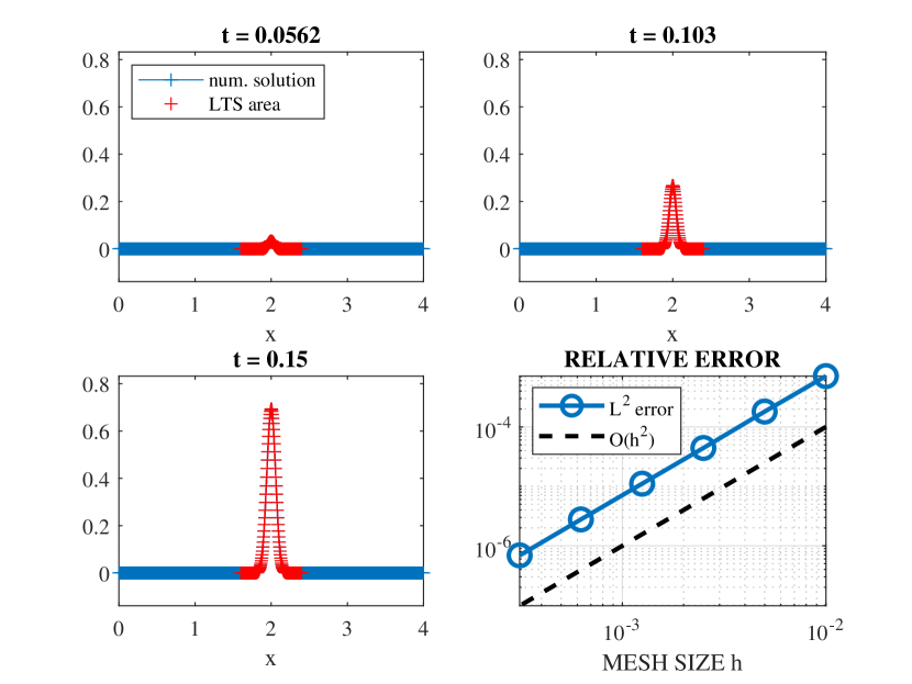
4 Towards Optimal H1superscript𝐻1H^{1} Convergence

The LF-LTS(ν𝜈\nu) Algorithm 1 achieves the optimal convergence rate 𝒪(Δt2+hm+1)𝒪Δsuperscript𝑡2superscript𝑚1{\cal O}(\Delta t^{2}+h^{m+1}) with respect to the L2superscript𝐿2L^{2}-norm with piecewise polynomial FE of degree m𝑚m also in the presence of a source f𝑓f – see Theorem 7. In [6], however, it was shown that the original LF-LTS method from [21, Algorithm 1], that is, the LF-LTS(ν𝜈\nu) Algorithm 1 with ν=0𝜈0\nu=0, may not achieve the expected optimal convergence rate in the H1superscript𝐻1H^{1}-norm whenever the source f𝑓f is nonzero across the coarse-to-fine interface. To restore optimal H1superscript𝐻1H^{1}-convergence regardless of f𝑓f, we shall replace the somewhat abrupt projections from Section 2.2 by a new more gradual weighted transition.

Let the set of simplex vertices be denoted by 𝒱(𝒯)𝒱𝒯\mathcal{V}\left(\mathcal{T}\right) and let (𝒯)𝒯\mathcal{E}\left(\mathcal{T}\right) denote the set of edges if d2𝑑2d\geq 2 while for d=1𝑑1d=1 we set (𝒯)=𝒯𝒯𝒯\mathcal{E}\left(\mathcal{T}\right)=\mathcal{T}. The definition of S𝒯msuperscriptsubscript𝑆𝒯𝑚S_{\mathcal{T}}^{m} gives rise to the interpolation operator I𝒯m:C0(Ω¯)S𝒯m:superscriptsubscript𝐼𝒯𝑚superscript𝐶0¯Ωsuperscriptsubscript𝑆𝒯𝑚I_{\mathcal{T}}^{m}:C^{0}\left(\overline{\Omega}\right)\rightarrow S_{\mathcal{T}}^{m}. For example, for m=1𝑚1m=1 the space S𝒯1superscriptsubscript𝑆𝒯1S_{\mathcal{T}}^{1} consists of the continuous, piecewise linear polynomials and I𝒯1superscriptsubscript𝐼𝒯1I_{\mathcal{T}}^{1} is the nodal interpolant

I𝒯1u=z𝒱(𝒯)u(z)b1,z.superscriptsubscript𝐼𝒯1𝑢subscript𝑧𝒱𝒯𝑢𝑧subscript𝑏1𝑧.I_{\mathcal{T}}^{1}u=\sum_{z\in\mathcal{V}\left(\mathcal{T}\right)}u\left(z\right)b_{1,z}\text{.}

For two points y,z𝑦𝑧y,z in Euclidean space, we denote by [y,z]𝑦𝑧\left[y,z\right] the straight line connecting y𝑦y and z𝑧z.

Definition 1 (connecting sequence)

For y,z𝒱(𝒯)𝑦𝑧𝒱𝒯y,z\in\mathcal{V}\left(\mathcal{T}\right), a sequence 𝐱=(xi)i=0m𝒱(𝒯)𝐱superscriptsubscriptsubscript𝑥𝑖𝑖0𝑚𝒱𝒯\mathbf{x}=\left(x_{i}\right)_{i=0}^{m}\subset\mathcal{V}\left(\mathcal{T}\right) is a connecting sequence of y𝑦y and z𝑧z if

x0=y,xm=z,and for 1jm: [xj1,xj](𝒯).:formulae-sequencesubscript𝑥0𝑦formulae-sequencesubscript𝑥𝑚𝑧and for 1𝑗𝑚 subscript𝑥𝑗1subscript𝑥𝑗𝒯.x_{0}=y,\quad x_{m}=z,\quad\text{and for }1\leq j\leq m:\text{ }\left[x_{j-1},x_{j}\right]\in\mathcal{E}\left(\mathcal{T}\right)\text{.}

The length of 𝐱𝐱\mathbf{x} is length(𝐱):=massignlength𝐱𝑚\operatorname{length}\left(\mathbf{x}\right):=m.

Definition 2 (graph distance)

The graph distance between y,z𝒱(𝒯)𝑦𝑧𝒱𝒯y,z\in\mathcal{V}\left(\mathcal{T}\right) is given by

dist𝒯(y,z):=min{length(𝐱):𝐱 is a connecting sequence of y and z}.assignsubscriptdist𝒯𝑦𝑧:length𝐱𝐱 is a connecting sequence of 𝑦 and 𝑧\operatorname{dist}_{\mathcal{T}}\left(y,z\right):=\min\left\{\operatorname{length}\left(\mathbf{x}\right):\mathbf{x}\text{ is a connecting sequence of }y\text{ and }z\right\}.

The graph distance between 𝒯fsubscript𝒯f\mathcal{T}_{\operatorname{f}} and some z𝒱(𝒯)𝑧𝒱𝒯z\in\mathcal{V}\left(\mathcal{T}\right) is given by

dist(𝒯f,z):=miny𝒯fdist𝒯(y,z).assigndistsubscript𝒯f𝑧subscript𝑦subscript𝒯fsubscriptdist𝒯𝑦𝑧\operatorname{dist}\left(\mathcal{T}_{\operatorname{f}},z\right):=\min_{y\in\mathcal{T}_{\operatorname{f}}}\operatorname{dist}_{\mathcal{T}}\left(y,z\right).
Definition 3 (discrete distance function)

Let 𝒯𝒯\mathcal{T} be a conforming simplicial finite element mesh and let the subset 𝒯f𝒯subscript𝒯f𝒯\mathcal{T}_{\operatorname{f}}\subset\mathcal{T} be fixed. The discrete distance function for s𝑠s simplex layers about 𝒯fsubscript𝒯f\mathcal{T}_{\operatorname{f}}, s1𝑠subscriptabsent1s\in\mathbb{N}_{\geq 1}, is given as follows. For z𝒱𝑧𝒱z\in\mathcal{V}, its value is set to

ηs(z):=(1dist(𝒯f,z)s)+assignsubscript𝜂𝑠𝑧subscript1distsubscript𝒯f𝑧𝑠\eta_{s}\left(z\right):=\left(1-\frac{\operatorname{dist}\left(\mathcal{T}_{\operatorname{f}},z\right)}{s}\right)_{+}

with (x)+:=max{x,0}assignsubscript𝑥𝑥0\left(x\right)_{+}:=\max\left\{x,0\right\}. On ΩΩ\Omega, the function is then given by

ηs=z𝒱(𝒯)ηs(z)b1,z.subscript𝜂𝑠subscript𝑧𝒱𝒯subscript𝜂𝑠𝑧subscript𝑏1𝑧\eta_{s}=\sum_{z\in\mathcal{V}\left(\mathcal{T}\right)}\eta_{s}\left(z\right)b_{1,z}.
Definition 4 (fine/coarse mesh mapping)

The fine mesh mapping ΠfS:SS:superscriptsubscriptΠf𝑆𝑆𝑆\Pi_{\operatorname{f}}^{S}:S\rightarrow S and coarse mesh mapping ΠcS:SS:superscriptsubscriptΠc𝑆𝑆𝑆\Pi_{\operatorname{c}}^{S}:S\rightarrow S are given by

ΠfSu:=zΣuzηs(z)bzand ΠcS:=IΠfS.formulae-sequenceassignsuperscriptsubscriptΠf𝑆𝑢subscript𝑧Σsubscript𝑢𝑧subscript𝜂𝑠𝑧subscript𝑏𝑧assignand superscriptsubscriptΠc𝑆𝐼superscriptsubscriptΠf𝑆\Pi_{\operatorname{f}}^{S}u:=\sum_{z\in\Sigma}u_{z}\eta_{s}\left(z\right)b_{z}\quad\text{and\quad}\Pi_{\operatorname{c}}^{S}:=I-\Pi_{\operatorname{f}}^{S}. (4.1)
Remark 4

Note that the above definition of ΠfSsuperscriptsubscriptΠf𝑆\Pi_{\operatorname{f}}^{S} and ΠcSsuperscriptsubscriptΠc𝑆\Pi_{\operatorname{c}}^{S} generalizes the respective operators as defined in [20] and (2.11): For s=1𝑠1s=1, both definitions coincide whereas for s>1𝑠1s>1 the coarse-to-fine transition is now spread across several layers.

Algorithm 1 formally remains unchanged; however, the operators ΠfSsuperscriptsubscriptΠf𝑆\Pi_{\operatorname{f}}^{S} and ΠcSsuperscriptsubscriptΠc𝑆\Pi_{\operatorname{c}}^{S} have to replaced by the new definition (4.1). This comes at an extra cost since the local time stepping is applied in s𝑠s additional simplex layers around the original fine region ΩfsubscriptΩf\Omega_{\operatorname*{f}} as in (2.9) which are recursively defined by Ωf+1superscriptsubscriptΩf1\Omega_{\operatorname*{f}}^{+1} as in (2.9) and for r=2,s𝑟2𝑠r=2,\ldots s by

Ωf+r:=int({τ𝒯:τΩf+(r1)¯}).assignsuperscriptsubscriptΩf𝑟intconditional-set𝜏𝒯𝜏¯superscriptsubscriptΩf𝑟1\Omega_{\operatorname*{f}}^{+r}:=\operatorname*{int}\left(\bigcup{\left\{\tau\in\mathcal{T}:\tau\cap\overline{\Omega_{\operatorname*{f}}^{+\left(r-1\right)}}\neq\emptyset\right\}}\right).

In Section 5.2 we will report on numerical experiments for this modification.

5 Numerical Experiments

First, we present numerical experiments which corroborate the convergence theory from Section 3 and hence demonstrate that the LF-LTS(ν𝜈\nu) method for the inhomogeneous wave equation defined in Algorithm 1 achieves the expected optimal rates of convergence with respect to the L2superscript𝐿2L^{2} norm. In doing so, we also compare the LF-LTS method with the alternative “split-LFC” approach from [3], where the source inside the locally refined region is only evaluated once at each global time-step – see Remark 1.

Next, in Section 5.2, we show via two numerical experiments that the weighted transition, introduced in Section 4, indeed restores optimal H1superscript𝐻1H^{1}-convergence regardless of the source and its position with respect to the refined region in the mesh.

5.1 Optimal L2superscript𝐿2L^{2} Convergence

We consider the one-dimensional wave equation (2.4) in Ω=(0,4)Ω04\Omega=(0,4) with homogeneous Dirichlet boundary conditions, i.e. Γ=ΓDΓsubscriptΓ𝐷\Gamma=\Gamma_{D}, c1𝑐1c\equiv 1, and inhomogeneous source term

f(x,t)=250e400((x2)2+(t0.1)2),𝑓𝑥𝑡250superscript𝑒400superscript𝑥22superscript𝑡0.12f(x,t)=250\,e^{-400\left(\left(x-2\right)^{2}+\left(t-0.1\right)^{2}\right)}, (5.1)

a narrow space-time Gaussian pulse centered about x=2𝑥2x=2 and t=0.1𝑡0.1t=0.1. The initial conditions are set to zero, i.e., u00subscript𝑢00u_{0}\equiv 0, v00subscript𝑣00v_{0}\equiv 0.

For the numerical solution, we use piecewise linear H1superscript𝐻1H^{1}-conforming finite elements with mass-lumping in space and the LF-LTS(ν𝜈\nu) method with global time-step Δt=eνhcΔ𝑡superscripte𝜈subscriptc\Delta t=\operatorname*{e}^{-\nu}h_{\operatorname*{c}} and ν=0.01𝜈0.01\nu=0.01 in time. Next, we split the computational domain ΩΩ\Omega into a coarse part, Ωc=(0,1.6)(2.4,4)subscriptΩc01.62.44\Omega_{\operatorname*{c}}=(0,1.6)\cup(2.4,4), and a locally refined part, Ωf=[1.6,2.4]subscriptΩf1.62.4\Omega_{\operatorname*{f}}=[1.6,2.4], inside each of which we use an equidistant mesh with mesh sizes hcsubscriptch_{\operatorname*{c}} or hf=hc/2subscriptfsubscriptc2h_{\operatorname*{f}}=h_{\operatorname*{c}}/2, respectively. Hence inside ΩfsubscriptΩf\Omega_{\operatorname*{f}}, the LF-LTS(ν𝜈\nu) method takes p=2𝑝2p=2 local time-steps of size Δt/pΔ𝑡𝑝\Delta t/p for each global time-step of size ΔtΔ𝑡\Delta t.

In Fig. 1, we display the LF-LTS(ν𝜈\nu) numerical solution for hc=0.01subscriptc0.01h_{\operatorname*{c}}=0.01 at times t0.05𝑡0.05t\approx 0.05, t0.1𝑡0.1t\approx 0.1, and t=0.15𝑡0.15t=0.15, together with the relative L2superscript𝐿2L^{2}-error at t=0.15𝑡0.15t=0.15 for a sequence of locally refined meshes. The L2superscript𝐿2L^{2}-error indeed displays the expected optimal second-order convergence rate 𝒪(hc2)𝒪superscriptsubscriptc2\mathcal{O}\left(h_{\operatorname*{c}}^{2}\right), as proved in Theorem 7.

Refer to caption
Figure 1: Snapshots of the LF-LTS(ν𝜈\nu) solution of (2.4) with ν=0.01𝜈0.01\nu=0.01 and f𝑓f as in (5.1) (top left, top right and bottom left). Relative L2superscript𝐿2L^{2}-error vs. h=hcsubscriptch=h_{\operatorname*{c}} for 1subscript1\mathbb{P}_{1} finite elements (bottom right).

In Fig. 2, that same relative L2superscript𝐿2L^{2}-error is compared to that of the alternative approach from [3], denoted here by LFC-LTS, which omits the intermediate source evaluations inside the refined region. Although both methods converge with the optimal rate 𝒪(hc2)𝒪superscriptsubscriptc2\mathcal{O}\left(h_{\operatorname*{c}}^{2}\right), as expected, the LF-LTS(ν𝜈\nu) algorithm from Section 2.3 here yields a threefold reduction in the error.

Refer to caption
Figure 2: L2superscript𝐿2L^{2}-error vs. h=hcsubscriptch=h_{\operatorname*{c}}: LF-LTS(ν𝜈\nu) method (3.20) (dash-dotted red line) and alternative “split LFC” approach from [3] – see Remark 1 (solid blue line).

5.2 Optimal H1superscript𝐻1H^{1}-Convergence and weighted transition

In [6], it was shown for a particular (spatially constant) source term f𝑓f that the original LF-LTS method from [21, Algorithm 1], that is, the LF-LTS(ν𝜈\nu) Algorithm 1 with ν=0𝜈0\nu=0, may not always achieve the expected optimal convergence rate in the H1superscript𝐻1H^{1}-norm. Here, we carefully study this behavior for two different source terms and show that the weighted transition from Section 4 restores the optimal H1superscript𝐻1H^{1}-convergence regardless of f𝑓f.

5.2.1 Space-time local forcing

Again, we consider the wave equation (2.4) with zero initial conditions and source f𝑓f as in (5.1) from the previous section. For spatial discretization, however, we use piecewise quadratic H1superscript𝐻1H^{1}-conforming finite elements with mass-lumping (2subscript2\mathbb{P}_{2}-FE). The computational domain separates into a coarse part ΩcsubscriptΩc\Omega_{\operatorname*{c}} and a locally refined part ΩfsubscriptΩf\Omega_{\operatorname*{f}} with corresponding mesh sizes hcsubscriptch_{\operatorname*{c}} or hf=hc/5subscriptfsubscriptc5h_{\operatorname*{f}}=h_{\operatorname*{c}}/5, respectively.

Now, while keeping the source fixed, we shall progressively shift the location of the refined region rightward and thus mimic the following three distinct situations: (i) source f𝑓f located entirely inside ΩfsubscriptΩf\Omega_{\operatorname*{f}}, (ii) source f𝑓f nonzero across coarse-to-fine mesh interface, (iii) source f𝑓f located entirely inside ΩcsubscriptΩc\Omega_{\operatorname*{c}}. In each case we monitor the H1superscript𝐻1H^{1}-convergence rates of the LF-LTS(ν𝜈\nu) method for p=5𝑝5p=5 and ν=0.01𝜈0.01\nu=0.01 either with, or without, weighted transition. Hence the fine mesh mapping ΠfSsubscriptsuperscriptΠ𝑆f\Pi^{S}_{\operatorname*{f}} is either defined by (4.1) with weighted transition across s1/hcsimilar-to𝑠1subscriptcs\sim 1/h_{\operatorname*{c}} elements, or without weighted transition, i.e., as in (4.1) with s=1𝑠1s=1 – see also Remark 4.

First, we set Ωf=[1.6,2.4]subscriptΩf1.62.4\Omega_{\operatorname*{f}}=[1.6,2.4] so that the support of f𝑓f completely lies inside ΩfsubscriptΩf\Omega_{\operatorname*{f}} (up to machine precision), as illustrated in Fig. 3. Here, the LF-LTS(ν𝜈\nu) method achieves the optimal second-order rate 𝒪(hc2)𝒪superscriptsubscriptc2\mathcal{O}(h_{\operatorname*{c}}^{2}) both with, or without, weighted transition, as shown in Fig. 3. Recall that overall second-order convergence vs. hcsubscriptch_{\operatorname*{c}} (or ΔtΔ𝑡\Delta t) in the H1superscript𝐻1H^{1}-norm is expected here since we use 2subscript2\mathbb{P}_{2}-FE in space.

Refer to caption
Refer to caption
Figure 3: Left: Source f(x,t)𝑓𝑥𝑡f(x,t) for different times t𝑡t, inside locally refined mesh with Ωf=[1.6,2.4]subscriptΩf1.62.4\Omega_{\operatorname*{f}}=[1.6,2.4]. Right: Relative H1superscript𝐻1H^{1}-error with (pink solid line), or without (blue dash-dotted line), weighted transition vs. mesh size h=hcsubscriptch=h_{\operatorname*{c}}.

Next, we shift the locally refined part rightwards and set Ωf=[2,2.4]subscriptΩf22.4\Omega_{\operatorname*{f}}=[2,2.4] so that f𝑓f is non-zero across the interface between ΩfsubscriptΩf\Omega_{\operatorname*{f}} and ΩcsubscriptΩc\Omega_{\operatorname*{c}}, as shown in Fig. 4; in fact, the coarse-to-fine mesh interface now coincides with the maximum of f𝑓f at x=2𝑥2x=2. In Fig. 4, we observe that the LF-LTS(ν𝜈\nu) method without weighted transition only converges as 𝒪(hc1.5)𝒪superscriptsubscriptc1.5\mathcal{O}(h_{\operatorname*{c}}^{1.5}), while using the weighted transition across s1/hcsimilar-to𝑠1subscriptcs\sim 1/h_{\operatorname*{c}} layers of elements restores the expected optimal second-order convergence.

Refer to caption
Refer to caption
Figure 4: Left: Source f(x,t)𝑓𝑥𝑡f(x,t) for different times t𝑡t, nonzero across coarse-to-fine mesh interface with Ωf=[2,2.4]subscriptΩf22.4\Omega_{\operatorname*{f}}=[2,2.4]. Right: Relative H1superscript𝐻1H^{1}-error with (pink solid line), or without (blue dash-dotted line), weighted transition vs. mesh size h=hcsubscriptch=h_{\operatorname*{c}}.

Finally, we shift the locally refined part even farther to the right and set Ωf:=[2.2,2.4]assignsubscriptΩf2.22.4\Omega_{\operatorname*{f}}:=[2.2,2.4] so that the support of the source term essentially lies inside the coarse part of the mesh, as shown in Fig. 5. Here, as in the first case, we again observe optimal second-order convergence in the H1superscript𝐻1H^{1}-norm, be it with or without weighted transition.

Refer to caption
Refer to caption
Figure 5: Left: Source f(x,t)𝑓𝑥𝑡f(x,t) for different times t𝑡t, outside locally refined region with Ωf=[2.2,2.4]subscriptΩf2.22.4\Omega_{\operatorname*{f}}=[2.2,2.4]. Right: Relative H1superscript𝐻1H^{1}-error with (pink solid line), or without (blue dash-dotted line), weighted transition vs. mesh size h=hcsubscriptch=h_{\operatorname*{c}}.

In summary, the LF-LTS(ν𝜈\nu) method without weighted transition achieves in the considered examples the expected optimal convergence rates in the H1superscript𝐻1H^{1}-norm when the source vanishes at the coarse-to-fine mesh transition; otherwise, when the source is non-zero across the mesh interface, the H1superscript𝐻1H^{1}-convergence rate is reduced by one half. The weighted transition introduced in Section 4 restores the expected optimal H1superscript𝐻1H^{1}-convergence even when f𝑓f is nonzero across the coarse-to-fine mesh interface.

5.2.2 Spatially constant solution

Finally, we revisit the example from [6, Section 7.1.3] and consider the wave equation (2.4) in Ω=(0,1)Ω01\Omega=(0,1) with homogeneous Neumann boundary conditions and zero initial conditions. Hence, we set the right-hand side f𝑓f as in [6] such that the solution is given by the spatially constant function

u(x,t)={0,t0.1,11+e0.8(1t0.1+1t0.9),0.1<t<0.9,1,t0.9.u(x,t)=\left\{\begin{aligned} &0,&&t\leq 0.1,\\ &\frac{1}{1+\operatorname*{e}^{0.8\left(\frac{1}{t-0.1}+\frac{1}{t-0.9}\right)}},&&0.1<t<0.9,\\ &1,&&t\geq 0.9.\end{aligned}\right. (5.2)

Now, we discretize (2.4) with 2subscript2\mathbb{P}_{2}-FE in space and the LF-LTS(ν𝜈\nu) Algorithm 1 with ν=0.01𝜈0.01\nu=0.01 in time. The refined region is (arbitrarily) set to the right half of the computational domain as Ωf=[0.5,1]subscriptΩf0.51\Omega_{\operatorname*{f}}=[0.5,1] with a coarse-to-fine mesh size ratio of p=2𝑝2p=2. Clearly, here the spatially constant source is nonzero across the coarse-to-fine mesh transition.

Refer to caption
Refer to caption
Figure 6: Relative L2superscript𝐿2L^{2}- and H1superscript𝐻1H^{1}-errors without (top), or with (bottom), weighted transition.

In Figure 6, we compare the L2superscript𝐿2L^{2}- and H1superscript𝐻1H^{1}-errors on a sequence of meshes of size h=hcsubscriptch=h_{\operatorname*{c}} either with, or without, weighted transition. Although the L2superscript𝐿2L^{2}-convergence theory from Section 3 does not apply here due to the Neumann boundary conditions, we still observe optimal second-order convergence both with or without weighted transition. Note that the overall second-order rate of convergence is dictated here by the time accuracy of the LF-LTS scheme. In contrast for the relative H1superscript𝐻1H^{1}-error, we observe an order reduction by h1/2superscript12h^{1/2} without weighted transition. By using the weighted transition across s1/hsimilar-to𝑠1s\sim 1/h element layers from Section 4, however, optimal second-order convergence is again restored – recall that 2subscript2\mathbb{P}_{2}-FE are used here for the spatial discretization.

To exhibit the mechanism that leads to this subtle order reduction by h1/2superscript12h^{1/2}, which only affects the H1superscript𝐻1H^{1} and not the L2superscript𝐿2L^{2}-convergence, we now strongly magnify in Fig. 7 the two (nearly constant) numerical solutions across the coarse-to-fine mesh transition for two different mesh sizes. Both variants of the LF-LTS(ν𝜈\nu) method, with or without weighted transition, introduce a small perturbation near x=0.5𝑥0.5x=0.5, whose amplitude tends to zero as h00h\rightarrow 0. Without weighted transition, however, this perturbation increasingly steepens as h00h\to 0, which results in increased gradients at the intersection of ΩcsubscriptΩc\Omega_{\operatorname*{c}} and ΩfsubscriptΩf\Omega_{\operatorname*{f}}. Hence the weighted transition prevents the formation of increasingly steep gradients as h00h\rightarrow 0 at the coarse-to-fine mesh meeting point and thus restores the expected optimal H1superscript𝐻1H^{1}-convergence.

Refer to caption
Refer to caption
Figure 7: Exact (dashed lines) and numerical solutions with (s1/hsimilar-to𝑠1s\sim 1/h, solid), or without (s=1𝑠1s=1, dash-dotted), weighted transition at t=0.29𝑡0.29t=0.29 with h=1.61021.6superscript102h=1.6\cdot 10^{-2} (top) or h=103superscript103h=10^{-3} (bottom).

Appendix A Appendix

Here we prove some technical estimates about Chebyshev polynomials.

Lemma 8

Let δp,νsubscript𝛿𝑝𝜈\delta_{p,\nu} be as in (2.12) and 0mnp10𝑚𝑛𝑝10\leq m\leq n\leq p-1. Then

|Un(m)(δp,ν)|(n+1)2m+1eν/2(2m+1)!!.superscriptsubscript𝑈𝑛𝑚subscript𝛿𝑝𝜈superscript𝑛12𝑚1superscripte𝜈2double-factorial2𝑚1\left|U_{n}^{\left(m\right)}\left(\delta_{p,\nu}\right)\right|\leq\frac{\left(n+1\right)^{2m+1}\operatorname*{e}^{\nu/2}}{\left(2m+1\right)!!}. (A.1)

An estimate from below is given by

Un(m)(δp,ν)2mm!(n+m+1nm)(2νp2)msuperscriptsubscript𝑈𝑛𝑚subscript𝛿𝑝𝜈superscript2𝑚𝑚binomial𝑛𝑚1𝑛𝑚superscript2𝜈superscript𝑝2𝑚U_{n}^{\left(m\right)}\left(\delta_{p,\nu}\right)\geq 2^{m}m!\binom{n+m+1}{n-m}\left(\frac{2\nu}{p^{2}}\right)^{m}

with the particular case

Un(δp,ν)n+1.subscript𝑈𝑛subscript𝛿𝑝𝜈𝑛1U_{n}\left(\delta_{p,\nu}\right)\geq n+1.

Proof. From [15, 18.9.21], we know that Un(m)=1n+1Tn+1(m+1)superscriptsubscript𝑈𝑛𝑚1𝑛1superscriptsubscript𝑇𝑛1𝑚1U_{n}^{\left(m\right)}=\frac{1}{n+1}T_{n+1}^{\left(m+1\right)} and (A.1) is equivalent to

Tn+1(m+1)(δp,ν)(n+1)2m+2eν/2(2m+1)!!.superscriptsubscript𝑇𝑛1𝑚1subscript𝛿𝑝𝜈superscript𝑛12𝑚2superscripte𝜈2double-factorial2𝑚1T_{n+1}^{\left(m+1\right)}\left(\delta_{p,\nu}\right)\leq\frac{\left(n+1\right)^{2m+2}\operatorname*{e}^{\nu/2}}{\left(2m+1\right)!!}.

The definition δp,ν=1+ν/p2subscript𝛿𝑝𝜈1𝜈superscript𝑝2\delta_{p,\nu}=1+\nu/p^{2} along the side constraints for m,n,p1𝑚𝑛𝑝1m,n,p-1 imply

δp,νδn+1,ν.subscript𝛿𝑝𝜈subscript𝛿𝑛1𝜈\delta_{p,\nu}\leq\delta_{n+1,\nu}.

Since Tn+1(m+1)(x)superscriptsubscript𝑇𝑛1𝑚1𝑥T_{n+1}^{\left(m+1\right)}\left(x\right) is increasing for x1𝑥1x\geq 1 we obtain from [20, Lem. A.1]

Tn+1(m+1)(δp,ν)Tn+1(m+1)(δn+1,ν)(n+1)2(m+1)eν/2(2m+1)!!.superscriptsubscript𝑇𝑛1𝑚1subscript𝛿𝑝𝜈superscriptsubscript𝑇𝑛1𝑚1subscript𝛿𝑛1𝜈superscript𝑛12𝑚1superscripte𝜈2double-factorial2𝑚1T_{n+1}^{\left(m+1\right)}\left(\delta_{p,\nu}\right)\leq T_{n+1}^{\left(m+1\right)}\left(\delta_{n+1,\nu}\right)\leq\frac{\left(n+1\right)^{2\left(m+1\right)}\operatorname*{e}^{\nu/2}}{\left(2m+1\right)!!}.

For the estimate from below we use the representation in [15, 18.7.4 and 18.5.7]

Un(m)(x)superscriptsubscript𝑈𝑛𝑚𝑥\displaystyle U_{n}^{\left(m\right)}\left(x\right) =m!2mn!(32)n=0n(n+2)(+3/2)n!(n)!(m)(x12)mabsent𝑚superscript2𝑚𝑛subscript32𝑛superscriptsubscript0𝑛subscript𝑛2subscript32𝑛𝑛binomial𝑚superscript𝑥12𝑚\displaystyle=\frac{m!}{2^{m}}\frac{n!}{\left(\frac{3}{2}\right)_{n}}\sum_{\ell=0}^{n}\frac{{\left(n+2\right)_{\ell}}{\left(\ell+3/2\right)_{n-\ell}}}{\ell!(n-\ell)!}\binom{\ell}{m}\left(\frac{x-1}{2}\right)^{\ell-m}
=2mm!=0n(n++1n)(m)(2(x1)).absentsuperscript2𝑚𝑚superscriptsubscript0𝑛binomial𝑛1𝑛binomial𝑚superscript2𝑥1\displaystyle=2^{m}m!\sum_{\ell=0}^{n}\binom{n+\ell+1}{n-\ell}\binom{\ell}{m}\left(2\left(x-1\right)\right)^{\ell}.

For x=δp,ν𝑥subscript𝛿𝑝𝜈x=\delta_{p,\nu}, this is a sum of positive terms and hence a lower bound is obtained by truncating it after the first non-zero term, i.e., for =m::𝑚absent\ell=m:

Un(m)(δp,ν)2mm!(n+m+1nm)(2νp2)m.superscriptsubscript𝑈𝑛𝑚subscript𝛿𝑝𝜈superscript2𝑚𝑚binomial𝑛𝑚1𝑛𝑚superscript2𝜈superscript𝑝2𝑚U_{n}^{\left(m\right)}\left(\delta_{p,\nu}\right)\geq 2^{m}m!\binom{n+m+1}{n-m}\left(\frac{2\nu}{p^{2}}\right)^{m}.


References

  • [1] G. A. Baker and V. A. Dougalis. The effect of quadrature errors on finite element approximations for second order hyperbolic equations. SIAM Journal on Numerical Analysis, 13(4):577–598, 1976.
  • [2] C. Carle and M. Hochbruck. Error analysis of multirate leapfrog-type methods for second-order semilinear ODEs. SIAM J. Numer. Anal., 60(5):2897–2924, 2022.
  • [3] C. Carle and M. Hochbruck. Error analysis of second-order local time integration methods for discontinuous Galerkin discretizations of linear wave equations. Math. Comp., 93(350):2611–2641, 2024.
  • [4] C. Carle, M. Hochbruck, and A. Sturm. On leapfrog-Chebyshev schemes. SIAM J. Numer. Anal., 58(4):2404–2433, 2020.
  • [5] J. Chabassier and S. Imperiale. Fourth-order energy-preserving locally implicit time discretization for linear wave equations. Internat. J. Numer. Methods Engrg., 106(8):593–622, 2016.
  • [6] Chabassier, Juliette and Imperiale, Sébastien. Construction and convergence analysis of conservative second order local time discretisation for linear wave equations. ESAIM: M2AN, 55(4):1507–1543, 2021.
  • [7] G. Cohen, P. Joly, J. E. Roberts, and N. Tordjman. Higher order triangular finite elements with mass lumping for the wave equation. SIAM J. Numer. Anal., 38(6):2047–2078, 2001.
  • [8] G. C. Cohen. Higher Order Numerical Methods for Transient Wave Equations. Springer Verlag, 2002.
  • [9] F. Collino, T. Fouquet, and P. Joly. A conservative space-time mesh refinement method for the 1-D wave equation. I. Construction. Numer. Math., 95(2):197–221, 2003.
  • [10] F. Collino, T. Fouquet, and P. Joly. A conservative space-time mesh refinement method for the 1-D wave equation. II. Analysis. Numer. Math., 95(2):223–251, 2003.
  • [11] F. Collino, T. Fouquet, and P. Joly. Conservative space-time mesh refinement methods for the FDTD solution of Maxwell’s equations. J. Comput. Phys., 211(1):9–35, 2006.
  • [12] S. Descombes, S. Lantéri, and L. Moya. Locally implicit discontinuous Galerkin method for time domain electromagnetics. J. Sci. Comp., 56:190–218, 2013.
  • [13] J. Diaz and M. J. Grote. Energy conserving explicit local time stepping for second-order wave equations. SIAM J. Sci. Comput., 31(3):1985–2014, 2009.
  • [14] J. Diaz and M. J. Grote. Multi-level explicit local time-stepping methods for second-order wave equations. Comput. Methods Appl. Mech. Engrg., 291:240–265, 2015.
  • [15] NIST Digital Library of Mathematical Functions. http://dlmf.nist.gov/, Release 1.0.13 of 2016-09-16. F. W. J. Olver, A. B. Olde Daalhuis, D. W. Lozier, B. I. Schneider, R. F. Boisvert, C. W. Clark, B. R. Miller and B. V. Saunders, eds.
  • [16] V. Dolean, H. Fahs, L. Fezoui, and S. Lanteri. Locally implicit discontinuous Galerkin method for time domain electromagnetics. J. Comput. Phys., 229:512–526, 2010.
  • [17] Ern, Alexandre and Guermond, Jean-Luc. Finite element quasi-interpolation and best approximation. ESAIM: M2AN, 51:1367–1385, 2017.
  • [18] J. C. Gilbert and P. Joly. Higher order time stepping for second order hyperbolic problems and optimal CFL conditions. In R. Glowinski and P. Neittaanmäki, editors, Partial Differential Equations, volume 16 of Comput. Methods Appl. Sci., pages 67–93. Springer-Verlag, Dordrecht, The Netherlands, 2008.
  • [19] M. J. Grote, M. Mehlin, and S. A. Sauter. Convergence analysis of energy conserving explicit local time-stepping methods for the wave equation. SIAM J. Numer. Anal., 56(2):994–1021, 2018.
  • [20] M. J. Grote, S. Michel, and S. A. Sauter. Stabilized leapfrog based local time-stepping method for the wave equation. Math. Comp., 90(332):2603–2643, 2021.
  • [21] M. J. Grote and T. Mitkova. Explicit local time-stepping methods for Maxwell’s equations. J. Comput. Appl. Math., 234(12):3283–3302, 2010.
  • [22] M. J. Grote, A. Schneebeli, and D. Schötzau. Discontinuous Galerkin finite element method for the wave equation. SIAM J. Numer. Anal., 44(6):2408–2431, 2006.
  • [23] M. Hochbruck and A. Sturm. Error analysis of a second-order locally implicit method for linear Maxwell’s equations. SIAM Journal on Numerical Analysis, 54(5):3167–3191, 2016.
  • [24] M. Hochbruck and A. Sturm. Upwind discontinuous Galerkin space discretization and locally implicit time integration for linear Maxwell’s equations. Math. Comp., 88(317):1121–1153, 2019.
  • [25] W. Hundsdorfer and J. Verwer. Numerical solution of time-dependent advection-diffusion-reaction equations, volume 33 of Springer Series in Computational Mathematics. Springer-Verlag, Berlin, 2003.
  • [26] P. Joly and J. Rodríguez. An error analysis of conservative space-time mesh refinement methods for the one-dimensional wave equation. SIAM J. Numer. Anal., 43(2):825–859, 2005.
  • [27] J. Lions and E. Magenes. Non-Homogeneous Boundary Value Problems and Applications. Springer-Verlag, Berlin, 1972.
  • [28] S. Minisini, E. Zhebel, A. Kononov, and W. A. Mulder. Local time stepping with the discontinuous Galerkin method for wave propagation in 3D heterogeneous media. Geophysics, 78:T67–T77, 2013.
  • [29] E. Montseny, S. Pernet, X. Ferriéres, and G. Cohen. Dissipative terms and local time-stepping improvements in a spatial high order Discontinuous Galerkin scheme for the time-domain Maxwell’s equations. J. Comput. Phys., 227:6795–6820, 2008.
  • [30] S. Piperno. Symplectic local time-stepping in non-dissipative DGTD methods applied to wave propagation problems. M2AN Math. Model. Numer. Anal., 40(5):815–841, 2006.
  • [31] M. Rietmann, M. J. Grote, D. Peter, and O. Schenk. Newmark local time stepping on high-performance computing architectures. J. Comput. Phys., 334:308–326, 2017.
  • [32] T. J. Rivlin. The Chebyshev Polynomials. Wiley, New York, 1974.
  • [33] J. G. Verwer. Component splitting for semi-discrete Maxwell equations. BIT, 51:427–445, 2011.