Exploring the three-dimensional momentum distribution
of longitudinally polarized quarks in the proton
The MAP (Multi-dimensional Analyses of Partonic distributions) Collaboration

Abstract

By analyzing experimental data on semi-inclusive deep inelastic scattering off longitudinally polarized targets, we extract the transverse momentum dependence of the quark helicity distribution, i.e., the difference between the three-dimensional motion of quarks with polarization parallel or antiparallel to the longitudinal polarization of the parent hadron. We perform the analysis at next-to-leading (NLL) and next-to-next-to-leading (NNLL) perturbative accuracy. The quality of the fit is very good for both cases, reaching a $\chi^{2}$ per number of data points equal to $1.11$ and $1.09$, respectively. Although the limited number of data points leads to significant uncertainties, the data are consistent with an interpretation in which the helicity distribution is narrower in transverse momentum than the unpolarized distribution.

I Introduction

Quarks are distributed inside the proton in an intricate way, determined by Quantum ChromoDynamics (QCD). The reconstruction of the distribution of quarks and gluons, encoded in the Parton Distribution Functions (PDFs) as a function of the longitudinal momentum fraction of the parent proton, $x$, is one of the most important achievements in the field of hadronic physics and has an impact on many sectors of physics, from precision studies of the Standard Model parameters, to the search for physics beyond the Standard Model, to cosmology Gross et al. (2023).

The distribution of quarks sharply depends on the orientation of their spins. The clearest example is provided by the so-called helicity distribution, i.e., the difference in the distribution of quarks with spin parallel ($q^{+}$) or antiparallel ($q^{-}$) to the spin of the proton when the proton is longitudinally polarized. We will use the notation $g_{1}^{q}(x)=q^{+}-q^{-}$ to denote the helicity distribution of quark $q$ and $f_{1}^{q}(x)=q^{+}+q^{-}$ to denote the unpolarized distribution. If we interpret PDFs as parton densitites, their positivity implies that $|g_{1}^{q}(x)|\leq f_{1}^{q}(x)$, which in turn prevents the polarized cross section to become negative (for a more detailed discussion, see Refs. de Florian et al. (2024); Candido et al. (2024)).

The helicity distribution has been determined in several works (see Refs. Nocera et al. (2014); Ethier and Nocera (2020); Bertone et al. (2024); Borsa et al. (2024) for recent extractions). The most salient features presently known can be summarized as follows: it is large and positive for $u$ quarks, large and negative for $d$ quarks. The helicity distribution is compatible with zero for antiquarks, and slightly positive for gluons. The distribution can be large, and even divergent at low $x$, but it is suppressed relative to the unpolarized distribution. On the contrary, at large $x$ the helicity distribution becomes as large as the unpolarized distribution and can saturate the positivity bound mentioned above. A detailed knowledge of the helicity distribution is crucial to separate the various contributions to the proton spin sum rule Ji (1997), and can indirectly provide evidence for the presence of partonic angular momentum (see, e.g., Refs. Ji et al. (2021); Leader and Lorcé (2014); Aidala et al. (2013) and references therein).

Up to now, the helicity distribution has been studied only as a function of $x$. But a new frontier in parton distribution studies is the determination of their dependence on the transverse momentum of quarks, encoded in Transverse Momentum Dependent PDFs (TMD PDFs). For instance, we would like to understand if quarks with spin parallel to the proton spin tend to have smaller or larger transverse momentum than quarks with antiparallel spin. The goal of the present work is to answer such kind of questions through the determination of the helicity TMD PDF from existing data. In our analysis, we use data measured by the HERMES Collaboration Airapetian et al. (2019) in Semi-Inclusive Deep Inelastic Scattering (SIDIS) with longitudinally polarized targets. Recent studies of other polarized TMD PDFs can be found in Refs. Cammarota et al. (2020); Bacchetta et al. (2022a); Echevarria et al. (2021); Bury et al. (2021); Boglione et al. (2021) for the Sivers function $f_{1T}^{\perp}$, in Refs. Kang et al. (2016); Cammarota et al. (2020); Gamberg et al. (2022); Boglione et al. (2024) for the transversity $h_{1}$, in Ref. Bhattacharya et al. (2022) for the worm-gear $g_{1T}$, and in Ref. Lefky and Prokudin (2015) for the pretzelosity $h_{1T}^{\perp}$.

For a consistent determination of any polarized TMD PDF, it is essential to start from a reliable extraction of the unpolarized TMD PDF and, when SIDIS data are involved, also of unpolarized TMD Fragmentation Functions (TMD FFs). Recent extractions of the unpolarized TMD PDF $f_{1}$ have been published in Refs. Bacchetta et al. (2017); Scimemi and Vladimirov (2018a); Bertone et al. (2019); Scimemi and Vladimirov (2020); Bacchetta et al. (2020); Bury et al. (2022); Bacchetta et al. (2022b); Moos et al. (2024); Bacchetta et al. (2024). The high level of perturbative accuracy reached in the theoretical framework and the large data sets analyzed with a very good quality of the fits are such that TMD PDFs have entered a precision era where they can potentially impact precision studies of Standard Model parameters like, e.g., the determination of the $W$ mass at hadron colliders Bacchetta et al. (2019). Recent extraction of the unpolarized TMD FF $D_{1}$ are presented in Refs. Bacchetta et al. (2017); Scimemi and Vladimirov (2020); Bacchetta et al. (2022b); Bacchetta et al. (2024). In this work, we choose to start from the MAPTMD22 extraction Bacchetta et al. (2022b) and we analyze the helicity TMD PDF with exactly the same formalism and computational framework Nan . We reach the next-to-next-to-leading (NNLL) level of logarithmic accuracy in resumming the soft gluon radiation, the highest presently achievable, but we discuss results also at NLL accuracy.

Our work is particularly relevant also because one of the main goals of existing and planned experimental facilities is to provide data to improve the determinations of the spin dependence of multi-dimensional quark distributions, including the helicity distribution Boer et al. (2011); Accardi et al. (2016); Dudek et al. (2012); Aschenauer et al. (2016); Accardi et al. (2024).

When this work was close to completion, an extraction of the helicity TMD PDF appeared in Ref. Yang et al. (2024). We briefly discuss the differences with this recent work at the end of Sec. III.

II Formalism

For the SIDIS process $\vec{e}+\vec{p}\to e^{\prime}+h+X$ involving the scattering of an electron and a proton, both longitudinally polarized, and the inclusive production of a hadron with fractional energy $z$ and transverse momentum $\bm{P}_{hT}$, the starting point of our analysis is the double spin asymmetry $A_{1}$. It is normally defined for inclusive DIS Diehl and Sapeta (2005); Filippone and Ji (2001), but it can be generalized to the SIDIS case at low transverse momentum using TMD factorization Ji et al. (2004); Collins (2013):

$$A_{1}(x,z,Q,|\bm{P}_{hT}|) =\frac{d\sigma^{\to\leftarrow}-d\sigma^{\to\to}+d\sigma^{\leftarrow\to}-d\sigma^{\leftarrow\leftarrow}}{d\sigma^{\to\leftarrow}+d\sigma^{\to\to}+d\sigma^{\leftarrow\to}+d\sigma^{\leftarrow\leftarrow}}$$

$$=\frac{\displaystyle\sum_{a=q,\bar{q}}e_{a}^{2}\int_{0}^{+\infty}d|\bm{b}_{T}||\bm{b}_{T}|\,J_{0}\left(\frac{|\bm{b}_{T}||\bm{P}_{hT}|}{z}\right)\hat{g}_{1}^{a}(x,\bm{b}_{T}^{2},Q)\hat{D}_{1}^{a\rightarrow h}(z,\bm{b}_{T}^{2},Q)}{\displaystyle\sum_{a=q,\bar{q}}e_{a}^{2}\int_{0}^{+\infty}d|\bm{b}_{T}||\bm{b}_{T}|\,J_{0}\left(\frac{|\bm{b}_{T}||\bm{P}_{hT}|}{z}\right)\hat{f}_{1}^{a}(x,\bm{b}_{T}^{2},Q)\hat{D}_{1}^{a\rightarrow h}(z,\bm{b}_{T}^{2},Q)}\,,$$ (1)

where the invariant mass $Q$ of the exchanged virtual photon is the hard scale of the SIDIS process, and $J_{0}$ is a Bessel function. The formula neglects power corrections of the type $\bm{P}_{hT}^{2}/z^{2}Q^{2}$ or $M^{2}/Q^{2}$. The denominator of Eq. (1) corresponds to the unpolarized cross section and involves the unpolarized TMD PDF $\hat{f}_{1}$ and TMD FF $\hat{D}_{1}$ in Fourier-conjugate $\bm{b}_{T}$-space, where the factorization formula is simpler. In principle, these functions should depend on two scales that usually are identified with the hard scale $Q$. In a similar way, the numerator of Eq. (1) involves the helicity TMD PDF $\hat{g}_{1}$.

Using the same prescriptions as in the MAPTMD22 analysis Bacchetta et al. (2022b), which are essentially based on the so-called Collins–Soper–Sterman (CSS) approach Collins et al. (1985); Collins (2013), the TMD PDFs $\hat{f}_{1}$ and $\hat{g}_{1}$ evolved from an arbitrary low scale $Q_{0}$ to the hard scale $Q$ can be written as

$$\hat{f}_{1}(x,\bm{b}_{T}^{2},Q) =\left[C^{f}\otimes f_{1}\right](x,b_{\ast}(\bm{b}_{T}^{2}))\,f_{\text{NP}}(x,\bm{b}_{T}^{2},Q_{0})\,e^{S(\mu_{b_{\ast}}^{2},Q^{2})}\ e^{g_{K}(\bm{b}_{T}^{2})\ln(Q^{2}/Q_{0}^{2})}\,,$$ (2)

$$\hat{g}_{1}(x,\bm{b}_{T}^{2},Q) =\left[C^{g}\otimes g_{1}\right](x,b_{\ast}(\bm{b}_{T}^{2}))\,g_{\text{NP}}(x,\bm{b}_{T}^{2},Q_{0})\,\,e^{S(\mu_{b_{\ast}}^{2},Q^{2})}\ e^{g_{K}(\bm{b}_{T}^{2})\ln(Q^{2}/Q_{0}^{2})}\,.$$ (3)

A similar formula holds also for the TMD FF $\hat{D}_{1}$. Using the Operator Product Expansion (OPE), the TMD PDFs $\hat{f}_{1}$, $\hat{g}_{1}$ can be matched onto the corresponding PDFs $f_{1}$ and $g_{1}$ through the Wilson coefficients $C^{f}$ and $C^{g}$, respectively. Both $C^{f}$, $C^{g}$ and the evolution operator $S$ can be calculated perturbatively. In this work, we reach the NLL and NNLL perturbative accuracy, according to Tab. 1 of Ref. Bacchetta et al. (2020). Note that for the numerator of Eq. (1) the NNLL level is the highest possible accuracy because the Wilson coefficients $C^{g}$ are known only up to order ${\cal O}(\alpha_{s})$ Gutiérrez-Reyes et al. (2017).

In Eqs. (2) and (3), $f_{\text{NP}}$, $g_{\text{NP}}$, $g_{K}$ are arbitrary nonperturbative functions that must be parametrized to experimental data. The scale $\mu_{b_{\ast}}$ is defined as $\mu_{b_{\ast}}=2e^{-\gamma_{E}}/b_{\ast}$, where $\gamma_{E}$ is the Euler constant, and $b_{\ast}$ is chosen according to an appropriate prescription. We take $f_{\text{NP}}$, $g_{K}$ and $b_{\ast}$ from the MAPTMD22 analysis Bacchetta et al. (2022b) (and similarly for the $D_{\text{NP}}$ of the TMD FF $\hat{D}_{1}$). We model the nonperturbative $g_{\text{NP}}$ in momentum space as the product of the nonperturbative $f_{\text{NP}}$ and a Gaussian with an $x$-dependent width:

$$g_{\text{NP}}(x,\bm{k}_{\perp}^{2},Q_{0})=\dfrac{f^{\text{MAP22}}_{\text{NP}}(x,\bm{k}_{\perp}^{2},Q_{0})\,e^{-\frac{\bm{k}_{\perp}^{2}}{w_{1}(x)}}}{k_{\text{norm}}(x)}\,,$$ (4)

where $\bm{k}_{\perp}$ is the transverse momentum of quarks with respect to the proton momentum direction, and $k_{\text{norm}}(x)$ depends on $w_{1}(x)$ and ensures that the integration over $\bm{k}_{\perp}$ of $g_{\text{NP}}$ equals unity (for convenience, the expression of $k_{\text{norm}}(x)$ is reproduced in Eq. (10)). The Gaussian width $w_{1}(x)$ has a crucial role in granting the positivity constraint $|g_{1}|\leq f_{1}$ also at the TMD level. In fact, by taking the ratio between the expressions in momentum space of Eq. (3) and Eq. (2) at the NLL level and at the initial scale $Q_{0}=1$ GeV, because of Eq. (4) we get

$$\frac{g_{1}(x,\bm{k}_{\perp}^{2},Q_{0})}{f_{1}(x,\bm{k}_{\perp}^{2},Q_{0})}=\frac{g_{1}(x,Q_{0})}{f_{1}(x,Q_{0})}\frac{e^{-\frac{\bm{k}_{\perp}^{2}}{w_{1}(x)}}}{k_{\text{norm}}(x)}\,.$$ (5)

For $|\bm{k}_{\perp}|\to 0$, the term $e^{-\bm{k}_{\perp}^{2}/w_{1}(x)}/k_{\text{norm}}(x)$ could potentially become very large, thus causing a possible violation of the positivity constraint unless we impose

$$\frac{g_{1}(x,Q_{0})}{f_{1}(x,Q_{0})}\frac{1}{k_{\text{norm}}(x)}\leq 1\,.$$ (6)

This condition implies that $w_{1}(x)$ must be bounded from below. Therefore, we choose

$$w_{1}(x)=f_{\text{pos.}}(x)+N_{1g}^{2}\frac{(1-x)^{\alpha_{1g}^{2}}x^{\sigma_{1g}}}{(1-\hat{x})^{\alpha_{1g}^{2}}\hat{x}^{\sigma_{1g}}}\,,$$ (7)

where $N_{1g},\,\alpha_{1g},\,\sigma_{1g}$ are free parameters and $\hat{x}=0.1$. The function $f_{\text{pos.}}(x)$ depends on the MAPTMD22 parameters, and it can be conveniently approximated as in Eq. (12). Eq. (6) is maintained for all values of $x$ in the analyzed range $[10^{-4},0.7]$. It also holds for higher values of $x$ if higher-order and target-mass corrections are neglected. However, since these corrections become significant in that region, we limit our analysis to the specified range $10^{-4}\leq x\leq 0.7$.

III Results

In this section, we present the key result of this study, the extraction of the helicity TMD PDF from a fit to SIDIS experimental data for the double spin asymmetry $A_{1}$ of Eq. (1). We use data for positive and negative charged pion/kaon production from deuterium and proton targets from the HERMES Collaboration Airapetian et al. (2019).

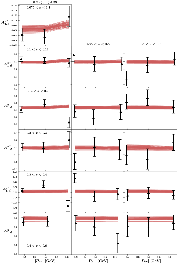
Figure 6: Comparison between HERMES asymmetry data and theoretical predictions (red lines) for the production of positive pion off a deuteron target for a selection of $x$ and $z$ bins. The results are reported as a function of the transverse momentum $|\bm{P}_{hT}|$ of the final-state hadron.

We apply the same kinematic cuts of the MAPTMD22 analysis Bacchetta et al. (2022b) in order to keep consistency with the unpolarized TMDs entering the denominator of $A_{1}$ and, more importantly, to fulfill the conditions for TMD factorization. Therefore, we do not include data on deuteron target from the COMPASS Collaboration (see Fig. 6 of Ref. Adolph et al. (2018)) nor data from the CLAS6 Collaboration Jawalkar et al. (2018) because they are not compatible with our kinematic cuts.

In total, we fit 291 data points. Our error analysis is performed with the so-called bootstrap method, namely by fitting an ensemble of Monte Carlo (MC) replicas of the experimental data. As in previous works of the MAP Collaboration Bacchetta et al. (2022b); Cerutti et al. (2023); Bacchetta et al. (2024), we consider the $\chi^{2}$ value of the best fit to the unfluctuated data as the most representative indicator of the quality of the fit. The data set has statistical and systematic uncertainties. We consider the former as uncorrelated while the latter as fully correlated. The expression of the $\chi^{2}$ contains a penalty term due to correlated uncertainties, that is described through nuisance parameters determined by minimizing the full $\chi^{2}$ on data (for more details see Refs. Bacchetta et al. (2022b); Cerutti et al. (2023); Bacchetta et al. (2024)).

For the denominator of the asymmetry $A_{1}$ in Eq. (1), we take the unpolarized TMD PDF $\hat{f}_{1}$ and TMD FF $\hat{D}_{1}$ from the MAPTMD22 extraction Bacchetta et al. (2022b). For the collinear polarized PDFs in Eq. (3), we choose the NNPDFpol1.1 set Nocera et al. (2014) with respect to more recent extractions Bertone et al. (2024); Borsa et al. (2024) because it includes parametrizations of $g_{1}$ also at lower perturbative order, that are needed for our analysis at NLL and NNLL accuracy. The NNPDFpol1.1 set contains 100 MC members. We generate the same number of replicas of the $A_{1}$ data points, we fit them, and we associate the $i$–th replica of the helicity PDF and the corresponding extracted helicity TMD PDF to the same replica of the unpolarized TMDs in the MAPTMD22 extraction. In this way, we propagate the uncertainty in the extraction of helicity PDFs onto the uncertainty of helicity TMD PDFs.

We perform our analysis at NLL and NNLL perturbative accuracy. The quality of the fit for both accuracies is shown in Table 1, where the $\chi^{2}$ per number of data points $N_{\rm dat}$ are listed for each considered experimental data set.

Experiment	$N_{\text{dat}}$	$\chi_{\text{NLL}}^{2}/N_{\text{dat}}$	$\chi_{\text{NNLL}}^{2}/N_{\text{dat}}$
HERMES ($d\rightarrow\pi^{+}$)	47	1.34	1.30
HERMES ($d\rightarrow\pi^{-}$)	47	1.10	1.08
HERMES ($d\rightarrow K^{+}$)	46	1.26	1.25
HERMES ($d\rightarrow K^{-}$)	45	0.93	0.89
HERMES ($p\rightarrow\pi^{+}$)	53	1.17	1.21
HERMES ($p\rightarrow\pi^{-}$)	53	0.86	0.86
Total	291	1.11	1.09

Table 1: Breakdown of $\chi^{2}$ per number of data points $N_{\text{dat}}$ for the best fits of HERMES data Airapetian et al. (2019) of double spin asymmetry $A_{1}$ in Eq. (1) at NLL and NNLL accuracy.

We note that the global quality of the fit slightly increases at higher accuracy. We also observe that the $\chi^{2}$ on the experimental data for the $\pi^{+}$ production are larger than for other fragmentation channels. The same feature was observed in the MAPTMD22 extraction of unpolarized quark TMDs Bacchetta et al. (2022b) and it is most likely related to the smaller experimental uncertainties in this fragmentation channel. In the Supplemental Material, we show the comparison between experimental data and results of the fit for all kinematic bins.

Parameters	$N_{1g}$	$\alpha_{1g}$	$\sigma_{1g}$
NLL	$0.70\pm 0.54$	$27.81\pm 27.70$	$0.42\pm 0.86$
NNLL	$0.87\pm 0.72$	$6.73\pm 6.58$	$3.04\pm 3.09$

Table 2: Average values and uncertainties (68% C.L.) of the free parameters in the helicity TMD PDF at NLL and NNLL accuracy.

In Tab. 2, we show the mean average values and associated errors at 68% confidence level (C.L.) for the free parameters in Eq. (7) at both NLL and NNLL accuracy. We note that in both cases the free parameters are poorly constrained. This is a consequence of the small number of available experimental data.

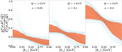
Figure 1: Ratio between the helicity and unpolarized TMD PDFs for quark $u$ in a proton at NNLL as a function of the quark transverse momentum $|\bm{k}_{\perp}|$, at $Q=1$ GeV and for $x=0.05$ (left panel), $x=0.1$ (central panel), and $x=0.3$ (right panel). Light blue lines for all replicas of the fit, orange band represents the 68% C.L.

In Fig. 1, we show the ratio between the helicity and the unpolarized TMD PDFs for a quark $u$ in a proton at NNLL, as a function of the quark transverse momentum $|\bm{k}_{\perp}|$ at $Q=1$ GeV and for $x=0.05$ (left panel), $x=0.1$ (central panel), and $x=0.3$ (right panel). The light blue lines represent all the replicas of our fit, while the orange band includes only 68% of them, obtained by excluding for each bin the largest and smallest 16% of them. We note that the $|\bm{k}_{\perp}|$ distribution of the ratio depends on $x$. At relatively small $x$, the ratio is almost flat: the shape of the $|\bm{k}_{\perp}|$ distribution of helicity and unpolarized TMD PDFs is approximately the same, the former being just rescaled from the latter. At larger $x$, the trend is different showing that the helicity TMD PDF has a sharper $|\bm{k}_{\perp}|$ distribution than the unpolarized one.

In the last years, efforts have been made to compute TMDs with lattice QCD (see Ref. Constantinou et al. (2021) and references therein). In order to make a comparison between our phenomenological extraction and lattice calculations, in Fig. 2 we show the ratio between helicity and unpolarized TMD PDFs for the valence quark $u_{v}$, integrated over $x$ as a function of $|\bm{k}_{\perp}|$ at $Q=2$ GeV. The orange lines represent all the replicas of our fit at NNLL (orange band for the 68% C.L.). The yellow and blue bands show the results of the lattice calculation of Ref. Musch et al. (2011). All the curves from our extraction are obtained by a numerical integration in the range $10^{-3}\leq x\leq 0.9$ in order to avoid numerical issues at the endpoints.

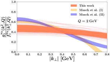
Figure 2: Ratio between the helicity and unpolarized TMD PDFs for valence $u_{v}$ quark integrated upon $x$, as a function of $|\bm{k}_{\perp}|$ at $Q=2$ GeV. Orange lines for all replicas of this fit at NNLL (orange band for the 68% C.L.), yellow and blue bands for the lattice calculations of Ref. Musch et al. (2011).

We observe that the result of our phenomenological extraction is in fair agreement with the lattice calculation but have a milder slope. A similar result is obtained at NLL accuracy. Further studies on the comparison with lattice results are certainly needed to assess the compatibility between the two different approaches.

While approaching the completion of this work, another extraction of the helicity TMD PDF appeared in Ref. Yang et al. (2024). The main differences with our extraction are twofold. First, the authors of Ref. Yang et al. (2024) implement the scale dependence of TMDs using the $\zeta$-prescription Scimemi and Vladimirov (2018b) rather than the CSS approach Collins (2013) used in Eqs. (2) and (3). Second, they include in the fit the CLAS6 experimental data and apply a more conservative transverse momentum cut to HERMES data, resulting in a smaller total number of analyzed data points compared to our work. More importantly, the authors of Ref. Yang et al. (2024) modify the $x$ dependence of the collinear helicity PDF. This has two important consequences: it breaks the matching between helicity PDF and TMD PDF in the OPE formula, and it implies that the integral over $\bm{k}_{\perp}$ of the helicity TMD PDF does not reproduce the helicity PDF, even at NLL. As a final remark, the positivity constraint $|g_{1}|\leq f_{1}$ is not enforced on the extracted helicity TMD PDF, and indeed it appears to be violated.

IV Conclusions

We have extracted the helicity TMD PDF of quarks from HERMES data Airapetian et al. (2019) for the double spin asymmetry in SIDIS kinematic conditions that satisfy the TMD factorization requirement. We evaluate the denominator of the asymmetry by using the unpolarized TMDs of the MAPTMD22 extraction Bacchetta et al. (2022b), and we consistently describe the helicity TMD PDF in the same framework reaching the NNLL perturbative accuracy, which is the current highest possible accuracy. We have parametrized the nonperturbative part of the helicity TMD PDF such that the positivity constraint is fulfilled by construction. Consistently with the MAPTMD22 extraction, we have performed the error analysis using the bootstrap method and correcting the $\chi^{2}$ expression with a penalty for correlated uncertainties. At large quark transverse momenta, the helicity TMD PDF can be matched onto the collinear helicity PDF through OPE. For the collinear helicity PDF, we have used the NNPDFpol1.1 set Nocera et al. (2014), and we have propagated the PDF uncertainties onto the TMD PDF by selecting a one-to-one correspondence between the replicas of the former and of the latter.

The quality of the fit is very good for both NLL and NNLL accuracies, reaching a $\chi^{2}$ per number of data points equal to $1.11$ and $1.09$, respectively. The shape of the transverse momentum distribution of the quark helicity TMD PDF shows a dependence on the longitudinal fractional momentum $x$ and tends to deviate from the one of the unpolarized TMD PDF at large $x$. Also, it nicely compares with the only lattice calculation available so far, after integrating upon $x$.

The nonperturbative part of the helicity TMD PDF is described by three free parameters which are poorly constrained because of the limited size of the experimental data set. New data from Jefferson Lab, as well as from the Electron-Ion Collider, will be important to refine the model of the arbitrary nonperturbative part of the helicity TMD PDF and, ultimately, to get more precise information regarding the spin content of the nucleon.

Appendix A Useful explicit formulas

We present here the expressions of all components that constitute the nonperturbative part of the helicity TMD PDF in Eq. (4). We begin by detailing the nonperturbative part employed in the MAPTMD22 analysis in $\bm{k}_{\perp}$ space:

$$f_{\text{NP}}^{\text{MAP22}}(x,\bm{k}_{\perp}^{2},Q_{0})=\frac{\exp\left(-\frac{\bm{k}_{\perp}^{2}}{g_{1A}(x)}\right)+\bm{k}_{\perp}^{2}\lambda^{2}\exp\left(-\frac{\bm{k}_{\perp}^{2}}{g_{1B}(x)}\right)+\lambda_{2}^{2}\exp\left(-\frac{\bm{k}_{\perp}^{2}}{g_{1C}(x)}\right)}{\pi\left(g_{1A}(x)+\lambda^{2}g_{1B}(x)^{2}+\lambda_{2}^{2}\,g_{1C}(x)\right)}\,,$$ (8)

where the $x$-dependent gaussian widths are defined as

$$g_{\{1A,1B,1C\}}(x)=N_{\{1,2,3\}}\frac{(1-x)^{\alpha^{2}_{\{1,2,3\}}}\,x^{\sigma_{\{1,2,3\}}}}{(1-\hat{x})^{\alpha^{2}_{\{1,2,3\}}}\,\hat{x}^{\sigma_{\{1,2,3\}}}}\,,$$ (9)

with $\hat{x}=0.1$. The $N_{i},,\alpha_{i},\,\sigma_{i}$ ($i=1,2,3$) and $\lambda_{j}$ ($j=1,2$) are the parameters extracted at NLL and NNLL in the MAPTMD22 work Bacchetta et al. (2022b) and they are available in the public NangaParbat repository.

The factor $k_{\text{norm}}(x)$, introduced to ensure the normalization of the non-perturbative part, is given by the following expression:

$$k_{\text{norm}}(x)=w_{1}(x)\frac{\frac{g_{1A}(x)}{g_{1A}(x)+w_{1}(x)}+\lambda^{2}\frac{g^{2}_{1B}(x)w_{1}(x)}{(g_{1B}(x)+w_{1}(x))^{2}}+\lambda_{2}^{2}\frac{g_{1C}(x)}{g_{1C}(x)+w_{1}(x)}}{g_{1A}(x)+\lambda^{2}g_{1B}^{2}(x)+\lambda_{2}^{2}g_{1C}(x)}.$$ (10)

This function depends on the MAPTMD22 parameters and on the function $w_{1}(x)$ defined in Eq. (7), which we reproduce here for convenience

$$w_{1}(x)=f_{\text{pos.}}(x)+N_{1g}\frac{(1-x)^{\alpha_{1g}^{2}}x^{\sigma_{1g}}}{(1-\hat{x})^{\alpha_{1g}^{2}}\hat{x}^{\sigma_{1g}}}\,.$$ (11)

The function $f_{\text{pos.}}(x)$ is chosen as a simple analytical formula

$$f_{\text{pos.}}(x)\approx c+h^{2}e^{-\frac{(x-\mu)^{2}}{\sigma^{2}}}\,,$$ (12)

where the values of the parameters $c$, $h^{2}$, $\mu$, and $\sigma$ will be available in the public NangaParbat repository Nan .

Appendix B Data/theory comparison plots

We report here the comparison of double spin asymmetries $A_{1}$ between our analysis and experimental data for all kinematic bins. The red lines all the MC replicas of the theoretical predictions.

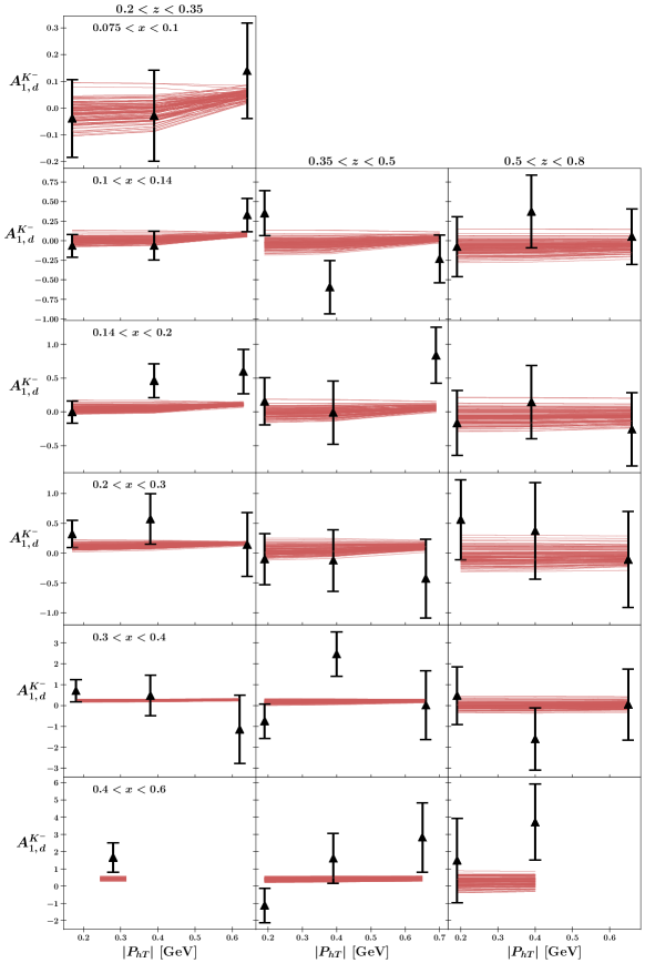
Figure 3: Comparison between HERMES asymmetry data and theoretical predictions (red lines) for the production of negative kaon off a deuteron target for a selection of $x$ and $z$ bins. The results are reported as a function of the transverse momentum $|\bm{P}_{hT}|$ of the final-state hadron.

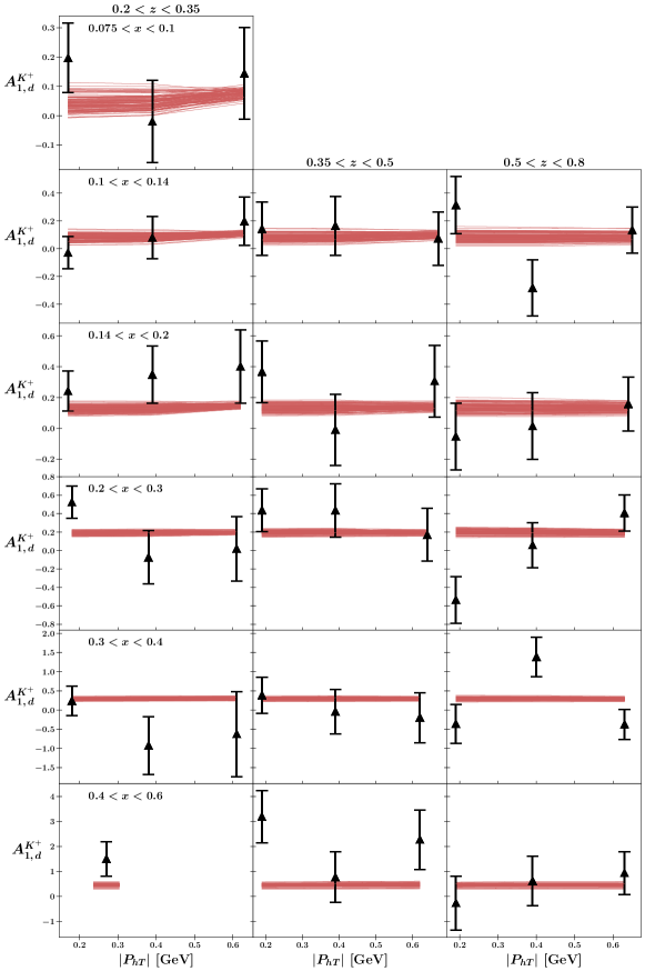
Figure 4: Comparison between HERMES asymmetry data and theoretical predictions (red lines) for the production of positive kaon off a deuteron target for a selection of $x$ and $z$ bins. The results are reported as a function of the transverse momentum $|\bm{P}_{hT}|$ of the final-state hadron.

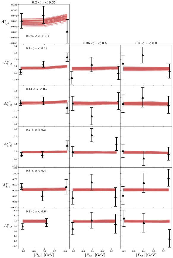
Figure 5: Comparison between HERMES asymmetry data and theoretical predictions (red lines) for the production of negative pion off a deuteron target for a selection of $x$ and $z$ bins. The results are reported as a function of the transverse momentum $|\bm{P}_{hT}|$ of the final-state hadron.

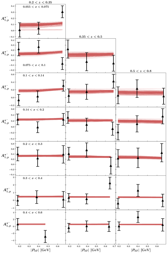
Figure 7: Comparison between HERMES asymmetry data and theoretical predictions (red lines) for the production of negative pion off a proton target for a selection of $x$ and $z$ bins. The results are reported as a function of the transverse momentum $|\bm{P}_{hT}|$ of the final-state hadron.

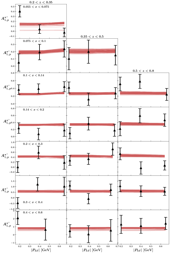
Figure 8: Comparison between HERMES asymmetry data and theoretical predictions (red lines) for the production of positive pion off a proton target for a selection of $x$ and $z$ bins. The results are reported as a function of the transverse momentum $|\bm{P}_{hT}|$ of the final-state hadron.