Classification and stability of penalized pinned elasticae
Abstract.
This paper considers critical points of the length-penalized elastic bending energy among planar curves whose endpoints are fixed. We classify all critical points with an explicit parametrization. The classification strongly depends on a special penalization parameter . Stability of all the critical points is also investigated, and again the threshold plays a decisive role. In addition, our explicit parametrization is applied to compare the energy of critical points, leading to uniqueness of minimal nontrivial critical points. As an application we obtain eventual embeddedness of elastic flows.
Key words and phrases:
Pinned elastica, bending energy, stability, elastic flow2020 Mathematics Subject Classification:
Primary: 53A04, Secondary: 49Q10, 53E401. Introduction
For an immersed planar curve , the bending energy (also known as the elastic energy) is defined by
where and respectively denote the signed curvature and the arclength parameter of . A critical point of the bending energy under the length-constraint is called Euler’s elastica, and it is known as a model of an elastic rod (cf. [2, 9, 13]).
In this paper we focus on the so-called modified (or length-penalized) bending energy
where is called a penalization parameter, and , which is an object of interest in the recent literature (see e.g. [1, 4, 10, 14, 16, 23, 24, 25] for studies of critical points, [5, 6, 7, 8, 15, 22] for gradient flows, and references therein).
In this paper we consider the critical points of under the so-called pinned boundary condition, which prescribes the endpoints up to zeroth order. More precisely, given , let
| (1.1) |
where denotes the set of -immersed curves, i.e.,
In this paper we call a critical point of in a penalized pinned elastica (see Definition 2.1 below).
The role of the modified bending energy depends on the penalization parameter . The larger is, the more dominant is the shortening role as opposed to the straightening effect. Taking this property into account, we ask the question
How does the penalization parameter affect the critical points of ?
Inspired by this question, we will obtain various properties of penalized pinned elasticae, such as (i) complete classification, (ii) stability results, (iii) uniqueness of nontrivial minimizers, and (iv) consequences for the elastic flow.
We first mention the complete classification of penalized pinned elasticae. To this end, we here introduce some functions involving the complete elliptic integrals: Let and be the functions defined by
| (1.2) | ||||
| (1.3) |
where and denote the complete elliptic integrals, which we introduce in Appendix A. Then, has a unique root (cf. Lemma 2.3) which is also a local maximum of with
| (1.4) |
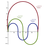
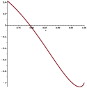
(see Lemma 2.4). Following terminology in Definition 2.7, we can classify penalized pinned elasticae as follows (see also Figure 1):
Theorem 1.1 (Classification for penalized pinned elasticae).
Let , , and
| (1.5) |
Suppose that is a critical point of in . Then, is a trivial line segment; otherwise, up to reflection and reparametrization, is represented by one of the following:
-
(i)
-shorter arc (denoted by ) for some integer ;
-
(ii)
-longer arc (denoted by ) for some integer ;
-
(iii)
-loop (denoted by ) for some integer .
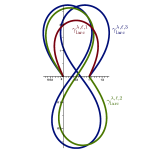
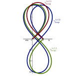
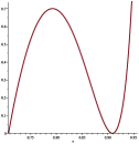
Explicit formulae for each penalized pinned elasticae are also obtained (see Definition 2.7 below). Note that the classification strongly depends on the relation of and defined in (1.4). More precisely, if , then holds so that and appear. On the other hand, if , then and coincide, and if , then holds so that and do not appear (see Figure 2). Such ‘bifurcation phenomena’ for elasticae have previously been found in [12, Section 2.3.3-2.3.5].
Next we address the stability (meaning here local minimality) of all the penalized pinned elasticae. The stability result we obtain again depends on the threshold .
Theorem 1.2 (Stability of penalized pinned elasticae).
Let be a penalized pinned elastica. If , then is stable if and only if is either a line segment or . Moreover, if , then is stable if and only if is a line segment. As a consequence, if , then there are exactly two local minimizers of in ; otherwise the local minimizer is unique.
A key tool to prove Theorem 1.2 is the analysis of the second variation. For instance, we show that is unstable by finding one perturbation whose second variation takes a negative value (see Lemma 3.5). In contrast, in order to show stability all possible perturbations need to be taken into account. However, it will turn out that in our situation it suffices to show positiveness of the second derivative along a certain perturbation of , not all perturbations (see the proof of Theorem 3.6). This substantial simplification is due to a minimizing property of in a different context from our setting.
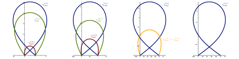
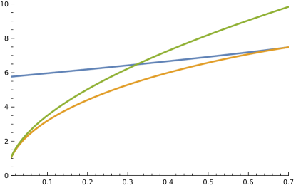
We also seek to compare the energies of the above critical points and study which one is energy-minimal (if one excludes the trivial line segment). As the explicit formulae show, and converge to as . This implies that for small it is not easy to determine which has less energy, or . On the other hand, for larger a comparison with is also required. Indeed, since
| (1.6) |
a comparison of needs to take into account the interaction of both summands. By a rigorous quantitative comparison of the energy, we obtain and for any (see Lemma 4.5 and Lemma 4.6, respectively). In addition, as a consequence of our energy-comparison result, we also obtain uniqueness of minimal nontrivial critical points as follows.
Theorem 1.3 (Uniqueness of nontrivial minimal penalized pinned elasticae).
Let and .
-
(i)
If , then is a unique minimizer of among nontrivial penalized pinned elasticae (up to reflection and reparametrization).
-
(ii)
If , then is a unique minimizer of among nontrivial penalized pinned elasticae (up to reflection and reparametrization).
Our results are applicable to the asymptotic analysis of the -gradient flow for , so-called -elastic flow, or simply elastic flow. The -elastic flow is defined by an -gradient flow of , and it is given by a one-parameter family of immersed curves such that
| (1.7) |
where denotes the curvature vector of , defined by , and denotes the normal derivative of a smooth vector field along . We consider the -elastic flow under the so-called natural (or Navier) boundary condition:
| (1.8) |
Here we are interested in the question of eventual embeddedness. We find a sharp energy threshold below which the above flow destroys any self-intersection in finite time. For more results on (not necessarily eventual) embeddedness of elastic flows we refer to [3, 17].
Theorem 1.4 (Eventual embeddedness of elastic flow).
Let and be a smooth curve satisfying (1.8). If
| (1.9) |
then there exists such that the -elastic flow with initial datum is embedded for all time .
The value is optimal in the sense that there is a smooth curve such that and the -elastic flow with initial datum is not embedded for all . Actually, one may choose . The instability of in Theorem 1.2 allows us to construct a nonembedded smooth curve satisfying the condition (1.9), cf. Remark 5.3. From Theorem 1.4 we then infer that the flow destroys each self-intersection of in finite time.
We close this introduction by comparing the properties of our penalized pinned elasticae with those already known from [19] about the critical points of in
where is given. It turns out that the curves of Theorem 1.1 are also critical points in if is chosen to be their corresponding length. In [19], stability of these curves in is investigated. A major difference is that depending on the choice of it is possible that is stable in , whereas this is never the case for our penalized problem (cf. Theorem 1.2). Another difference is that in stable critical points are always unique whereas for our penalized problem the number of stable critical points depends on . Exposing these differences to the fixed-length problem is a main novelty of the present article.
Organization
This paper is organized as follows: In Section 2 we give the complete classification of penalized pinned elasticae and prove Theorem 1.1. In Section 3 we investigate the stability (local minimality) of all penalized pinned elasticae to complete the proof of Theorem 1.2. In Section 4, we quantitatively compare the energy of penalized pinned elasticae, which yields the proof of Theorem 1.3. In Section 5 we apply our results in Section 2–4 to the analysis of the elastic flow.
Acknowledgments
This work was initiated during the second author’s visit at Freiburg University. The second author is very thankful to the first author for his warm hospitality and providing a fantastic research atmosphere. Both authors are grateful to Tatsuya Miura for helpful suggestions. The second author is supported by FMfI Excellent Poster Award 2022 and JSPS KAKENHI Grant Number 24K16951.
2. Classification
In this paper we define critical points of in in the following sense:
Definition 2.1.
We call a penalized pinned elastica if satisfies
-
(i)
;
-
(ii)
The first derivative vanishes for any perturbation of the kind with one has
(2.1)
Note that any local minimizer is a penalized pinned elastica. To begin with, we deduce the Euler–Lagrange equation and an additional (natural) boundary condition for penalized pinned elasticae.
Lemma 2.2 (The Euler–Lagrange equation and boundary condition).
Let be a penalized pinned elastica. Then, the signed curvature of the arclength reparametrization of is analytic on , where , and satisfies
| (2.2) | |||
| (2.3) |
Proof.
First we show that is smooth on . For arbitrary and consider for , where denotes the arclength function, i.e., . Inserting into (2.1), and using the known formulae of first derivative of and (cf. [18, Lemma A.1]), we deduce that
where and denote the unit tangent vector and the unit normal vector of , respectively. Since this identity holds in particular for all , we can deduce from a standard bootstrap argument that is of class .
Next we show that satisfies (2.2) and (2.3). Let be arbitrary and consider . With the help of integration by parts, we reduce (2.1) to
Considering arbitrary this implies that satisfies (2.2). In addition, by choosing with and , we deduce from the above relation that satisfies . Similarly we also obtain . Analyticity of immediately follows from the fact that satisfies the polynomial differential equation (2.2). ∎
For later use we exhibit some elementary properties of and , defined as in (1.2) and (1.3). In the following let denote the unique zero of , cf. Lemma A.1. The proof of Lemma 2.3 is postponed to Appendix B since it follows from a straightforward calculation.
Lemma 2.3.
Let be the function defined by (1.2). Then, there exists a unique such that
| (2.4) |
In addition, on and on .
The proof of the following lemma is safely omitted since it immediately follows from the definition of in (1.3).
Lemma 2.4.
Let be the function defined by (1.3). Then,
| (2.5) |
for . In addition, the function has exactly two local extrema at the points and . More precisely, is a unique local maximum and is a local minimum and is strictly monotone in , and .
Next we analytically estimate . The proof is postponed to Appendix B.
Lemma 2.5.
.
Now we define key moduli for classification of penalized pinned elasticae.
Definition 2.6.
Let be the constant given by (1.4).
-
(i)
For , let be the solutions to with
We interpret .
-
(ii)
For , let be a unique solution to .
Using these moduli, we prepare terminology for the following critical points. We will later show that these curves are indeed the only possibilities.
Definition 2.7 (Shorter arc, longer arc, and loop).
Let , , and be given, and let as in (1.5).
-
(i)
A curve is called -shorter arc if and if, up to reflection, the arclength parametrization of is given by
(2.6) (2.7) with length and signed curvature
-
(ii)
A curve is called -longer arc if and if, up to reflection, the arclength parametrization of is given by
(2.8) with length and signed curvature
-
(iii)
A curve is called -loop if, up to reflection, the arclength parametrization of is given by
(2.9) with length and signed curvature
In what follows we show Theorem 1.1 to verify that any penalized pinned elastica is either a -shorter arc, a -longer arc, or a -loop.
Proof of Theorem 1.1.
Let be a penalized pinned elastica and be the signed curvature of . Recall from Lemma 2.2 that satisfies (2.2) and (2.3). Then is a trivial solution to (2.2) and (2.3), so in the following we consider the other solutions. By [11, Proposition 3.3], any solution to the initial value problem for (2.2) with is given by
| (2.10) |
for some , , , and such that
| (2.11) |
Since we infer that . By (2.3) and antiperiodicity of (cf. Proposition A.3), we may choose in (2.10). Denote . In addition, we deduce from Lemma 2.2 that , which implies that
| (2.12) |
Next we use the boundary condition in the definition of , cf. (1.1), to gain more information about the parameters. We see from (2.10) that
where we used the well known integral formula of (cf. (A.3)). This implies that, up to rotation, the tangential angle of is given by
| (2.13) |
Then, up to rotation and translation, the arclength parametrization of is given by
| (2.14) |
Now we compute
| (2.15) | ||||
where we used (A.5) in the last equality. This together with (2.12) implies . Next we compute
| (2.16) | ||||
where we used (A.4) in the last equality. Thus we obtain . By (2.12) and the fact that for all , we also obtain
| (2.17) |
Note that follows from (2.15). Observe that by Lemma A.1 if and if . Then, combining the boundary condition with (2.14) and (2.17), we obtain
and observe that
| (2.18) |
is necessary to hold. Combining this together with (2.11), we see that
| (2.19) |
where is the function defined by (1.3). Thus needs to be either
By Lemma 2.4 is necessary if is either or .
Remark 2.8.
2.1. Properties of penalized pinned elasticae
Below we report on some geometric properties of penalized pinned elasticae, which can be deduced by explicit formulae in Theorem 1.1.
Lemma 2.9 (Symmetry of penalized pinned elasticae).
Let be either , , or and denote . Then, is reflectionally symmetric in the sense that satisfies
| (2.21) |
In addition, if , then has a self-intersection, i.e., there is such that .
Proof.
In the interest of brevity we only demonstrate the proof of the case of since the argument is fairly parallel in the other cases. We deduce from (2.9) that, for and ,
for all , where we used the evenness of . We also apply the oddness of and to obtain Since , we have
It remains to check that has a self-intersection. By reflectional symmetry, it suffices to find such that . Here recall from (2.13) and (2.20) that the tangential angle of is given by
Combining this with the fact that , we have
This implies that . Moreover, since and , we deduce from the intermediate value theorem that there exists such that . The proof is complete. ∎
3. Stability
In this section we address the question of stability of the penalized pinned elasticae found in Theorem 1.1. As mentioned in the introduction, in this paper stability means local minimality of in .
3.1. Stability of one-mode arcs
Here we focus on the stability of all penalized pinned elasticae with parameter
The following lemma ensures that under certain conditions it suffices to investigate the sign of the second derivative along one particular perturbation.
Lemma 3.1.
Let . Assume that there exists a perturbation of such that for some , such that ,
| (3.1) |
and the following properties hold:
-
(i)
the map is continuous and bijective;
-
(ii)
for each , a curve is a global minimizer of in
Then, is a stable penalized pinned elastica (i.e. a local minimizer of in ).
Proof.
By (3.1) (and the fact that the first derivative vanishes), we can find such that
| (3.2) |
We deduce from property (i) that there exists such that
| (3.3) |
Using the above , we now fix an arbitrary with . This implies in particular that . Property (i) also implies that there exists such that . From (3.3) follows that . Moreover, in view of property (ii), we see that , and this together with (3.2) yields that
which completes the proof. ∎
Thus it suffices to construct a perturbation of satisfying the assumption of Lemma 3.1. To this end we introduce a family which consists of wavelike elasticae.
Definition 3.2.
-
(i)
For , we define to be a curve whose length is and whose signed curvature is given by
(3.4) -
(ii)
For , we define to be a curve whose length is and whose signed curvature is given by
Notice that for each one has that is a wavelike elastica such that . The proof of this follows the lines of the proof of Theorem 1.1. Also note that, up to reparametrization,
| (3.5) |
Remark 3.3.
Here we show that satisfies assumptions (i) and (ii) in Lemma 3.1.
Lemma 3.4.
Let be a family defined in Definition 3.2. Then, the following properties hold.
-
(i)
The map is continuous and bijective.
-
(ii)
For each the curve is a minimizer of in
Proof.
Property (i) follows from the fact that is continuous and strictly decreasing (cf. [20, Lemma B.4]), and satisfies and .
Next we show property (ii). The curve coincides with in terms of [25, Theorem 1.1] since the modulus is uniquely determined by and since the signed curvature of is given by
(see [25, proof of Theorem 1.1] for the coincidence of the signed curvature). Then it follows from [25, Theorem 1.3] that is a minimizer of in . ∎
The following lemma ensures the sign of the second derivative of one-mode penalized pinned elasticae along the perturbation of .
Lemma 3.5.
Let and be a family defined in Definition 3.2. Then
In addition, the following properties hold.
-
(i)
If , then
(3.6) -
(ii)
If , then
(3.7) -
(iii)
For all and ,
(3.8)
Proof.
By (3.4) the bending energy of is represented by
The derivative formulae of elliptic integrals (cf. (A.1) and (A.2)) give
Recalling that , we have
where is given by (1.3). Thus, setting
we have
| (3.9) |
Since holds by definition (cf. Definition 2.6), it follows that for .
Next we compute the second derivative. It follows from (3.9) that
| (3.10) |
Note that the first term in the right-hand side of (3.10) vanishes for , , or . Note also that for all since (A.1) yields that and therefore
Therefore, we deduce from (3.10) that for
| (3.11) |
If , then combining (3.11) with Lemma 2.4 and the fact that , we obtain (3.6). If i.e., , then (3.11) combined with Lemma 2.4 implies that . By differentiating (3.10) and using the fact that and , we obtain
Thus in order to show (3.7) it suffices to check , which immediately follows from the derivative formula (2.5) of and the fact that and (cf. (B.3)). Finally, (3.8) follows by the combination of (3.11) with Lemma 2.4 and the fact that . The proof is complete. ∎
Theorem 3.6 (Stability of one-mode critical points).
Let be a penalized pinned elastica and denote its arclength parametrization.
-
(i)
If and , then is stable.
-
(ii)
If and , then is unstable.
-
(iii)
If and , then is unstable.
-
(iv)
If , then is unstable.
3.2. Instability of higher modes ()
In this subsection we show that , , and are unstable if . Combining this with the previous (in)stability results we are able to prove Theorem 1.2 in the end of this subsection.
We apply the general rigidity principles obtained in [19] to deduce the instability of , , and for . By Lemma 2.2 the bending energy satisfies [19, Hypotheses (H1’) and (H2)] with the choice of and clearly satisfies [19, Hypothesis (H3)]. This fact together with Remark 2.8 allows us to apply [19, Theorems 2.3, 2.7, and 2.8] to the case of and , , or .
Theorem 3.7 (Instability of more than two modes).
Let be a penalized pinned elastica. If the arclength parametrization of is represented by either , , or for some , then is not a local minimizer of in .
Proof.
Let be either , , or for some and . It follows from the formula of the signed curvature obtained in Theorem 1.1 that , so that satisfies [19, Assumption (2.2)]. Therefore, by [19, Theorem 2.3 and Remark 4.3] is not a local minimizer of in
The proof can now be concluded with the following claim.
| (3.12) | ||||
In fact, if is not a local minimizer of in , then there exists such that (as ) and for all . Since and , the family also satisfies and . This ensures that is also not a local minimizer of in . ∎
Theorem 3.8 (Instability of two modes).
Let be a penalized pinned elastica. If the arclength parametrization of is represented by either , , or , then is not a local minimizer of in .
Proof.
The proof of Theorem 1.2 is now already complete.
4. Energy comparison
Next we quantitatively compare the energy among penalized pinned elasticae and as a consequence deduce uniqueness of minimizers of among penalized pinned elasticae except for a trivial line segment.
To begin with we compute the energy of each penalized pinned elastica using the formulae in Definition 2.7.
Lemma 4.1.
Proof.
To compare the energy of each penalized pinned elastica, we prepare some functions to quantitatively characterize the energy as follows. Let and be defined by
| (4.3) | ||||
| (4.4) |
With the aid of the functions and one can provide two distinct formulae for the energies of penalized pinned elasticae. By Lemma 4.1 and (2.19) we see that
| (4.5) | ||||
which will be useful when we investigate how the energy depends on (see Lemma 4.4). On the other hand, since implies that , we have
| (4.6) | ||||
which will be useful for comparing the energy of and (see Lemma 4.5).
We exhibit some elementary properties of and in the following lemmas, whose proof is postponed to Appendix B.
Lemma 4.2.
Lemma 4.3.
Recall that we interpret the number as a mode. Therefore, as in [25], it will be naturally expected that, for instance, the energy gets larger if is larger. However, this does not directly follow since the moduli depend on the choice of , cf. Definition 2.7. In fact, combining the formula
| (4.10) |
with the fact that is increasing (cf. Definition 2.6), we see that is decreasing with respect to . This implies that consists of the increasing factor and the decreasing factor with respect to .
Nevertheless we can obtain the following monotonicity.
Lemma 4.4.
Let , , and . Let , , and be the curves defined in Definition 2.7. Then, if , the following inequalities hold:
| (4.11) |
Proof.
Here we show that holds for all .
Lemma 4.5 (Energy comparison of shorter arc and longer arc).
Proof.
First we show that (4.12) for the case and , i.e.,
| (4.13) |
Fix and define by
Hereafter we prove that for any and . Denote and for short. By Lemma 4.1, and the fact that , we deduce that
| (4.14) | ||||
where in the last equality we also used (4.10). Combining this with (2.5), we obtain
Since and are positive and strictly increasing with respect to (cf. Appendix A), we have for . Moreover, also follows since implies that . Thus we obtain (4.13), and equality holds if and only if , i.e., .
Next we consider the case . Fix arbitrarily. Setting and noting that then , we deduce from Lemma 4.1 that and , respectively. Moreover, noting that
| (4.15) |
and applying (4.13) to , we obtain
Equality in the above inequality holds if and only if , i.e., equality holds for all the inequalities in (4.15), which is equivalent to and . ∎
Lemma 4.6 (Energy comparison of one-mode longer arc and one-mode loop).
If and satisfy , then
On the other hand, the energy of with is higher than that of :
Lemma 4.7 (Energy comparison of higher-mode longer arc and one-mode loop).
Let , , and . Then,
We split the proof of Lemma 4.7 into two lemmas. First we investigate how the energy and depends on . Here recall from Theorem 1.1 that if exists then we have necessarily , i.e., . Also recall from (4.6) and Definition 2.7 that and .
Lemma 4.8.
Let , . Then, the map
| (4.16) |
is strictly decreasing on .
Proof.
Lemma 4.9.
For any and , the map defined by (4.16) satisfies
Proof.
In view of Lemma 4.8, it suffices to show that . By definition holds when . Throughout this proof write for short. Then, the problem is reduced to the positivity of . Since yields (after taking square roots) that
| (4.17) |
it follows that
Moreover, using (4.17) again, and noting that , we have
which leads to
where for the first term in the right-hand side we also used and monotonicity of . Thus we obtain
Set and hereafter we show that . Since is a solution of , satisfies . This yields
Note that since . By Lemma 2.5 and the fact that is a positive function, we also find that and hence
In order to deduce that , it suffices to show the positivity of
since . The fact that yields
Notice that is strictly increasing in . Indeed, the derivative has roots , implying that and . Due to this monotonicity we infer . The positivity of follows and the proof is complete. ∎
Now we turn to the proof of Lemma 4.7.
Proof of Lemma 4.7.
In addition, as follows one can observe the reversal of the order of the energy between and , depending on .
Lemma 4.10 (Energy comparison of one-mode shorter arc and one-mode loop).
Let and satisfy . Then, there exists a unique such that
In addition, if .
Proof.
Fix and define by
Then, the fact that and Lemma 4.6 yield that . Moreover, noting that and as , we deduce from the energy formulae (4.1) that
from which it follows that . Thus, for the desired conclusion it suffices to check that is strictly decreasing on . As in (4.14), we compute
Since yield and , we obtain
Then, in view of the fact that the map is strictly increasing, we find that the right-hand side in the above equation takes a negative value for all . The proof is complete. ∎
Remark 4.11.
This remark summarizes the insights gained in the previous lemmas in the important special case of small , i.e. . Notice that in this case one has . By Lemma 4.5 we have and by Lemma 4.6 we have . We infer
-
•
has minimal energy of all penalized pinned elasticae in (except for the line).
- •
-
•
Since increasing the mode makes the energy larger (cf. Lemma 4.4) we infer that all the elasticae with higher modes are not minimal.
We close this section by the proof of Theorem 1.3.
5. Elastic flow
In this section we apply our classification results in Theorem 1.1 and energy-comparison results in Lemmas 4.5 and 4.7 to the asymptotic behavior of the -elastic flow (1.7) under the Navier boundary conditions, cf. (1.8). It is already known that the solution to the flow subconverges to a stationary solution, which satisfies
| (5.1) |
We first recall the following statement (see e.g. [21, Section 2] or [15, Proposition 5.2]):
Proposition 5.1 (Long-time existence and subconvergence).
Let be a smoothly immersed curve such that . Then, there is a unique global-in-time smooth solution to the initial value problem,
Moreover, for any sequence there exist a subsequence and a smoothly immersed curve satisfying (5.1) such that converges smoothly to up to reparametrization.
The last subconvergence statement in Proposition 5.1 is slightly different from the original statement, but an inspection of the proofs in the above references immediately implies the above formulation. In view of Lemma 2.2, critical points of in in the sense of Definition 2.1 can be characterized by (5.1). Thus, stationary solutions of (5.1) correspond to critical points of in . Therefore, Theorem 1.1 can be also regarded as the complete classification of solutions to (5.1).
The classification and assumption (1.9) significantly reduce the candidates of trajectories of the elastic flow. In view of Lemmas 4.5 and 4.7, a non-trivial critical point of in whose energy is less than that of is either or , where and denotes the constant-speed reparametrization of and , respectively. Thus, recalling the fundamental property , we see that any limit curve must (after reparametrization) belong to
| (5.2) |
where denotes the unique line segment in . We interpret if since in this case and are absent.
To study embeddedness of the elastic flow it will be important to investigate whether a curve in is embedded.
Lemma 5.2.
Every curve is embedded.
Proof.
The case is trivial, so hereafter we consider . Then, it suffices to check embeddedness of and . Since the proof is completely parallel, we only consider . Set . We deduce from (2.6) that with and . As in (2.16) we obtain
Since , we see that is increasing for . Thus is convex in . This together with the fact that and implies that holds for all . By reflection symmetry (cf. (2.21)), it suffices to check embeddedness of for , which immediately follows from monotonicity of on . ∎
We are now ready to prove Theorem 1.4.
Proof of Theorem 1.4.
Let be the smooth evolution of the -elastic flow in with initial datum . We prove the theorem by contradiction. If the asserted time does not exist, then one can find a sequence such that is not embedded. By Proposition 5.1 we can find a subsequence and reparametrizations such that converges smoothly to some curve satisfying (5.1). By (5.2), we can choose the reparametrizations in such a way that must belong to . In particular, is embedded by Lemma 5.2. Since the set of embedded curves is open in the -topology, (which can e.g. be seen like in [20, Lemma 4.3]) and in the -topology, we obtain that must be embedded for some large . Since reparametrizations do not affect the embeddedness of a curve, we also have that must be embedded. A contradiction. ∎
Remark 5.3 (Extinction of a self-intersection).
Finally we remark that the energy threshold (1.9) is indeed undercut by curves that have a self-intersection. Theorem 1.4 yields then that for these curves, all the self-intersections become extinct in finite time. Here we give an explicit construction of nonembedded curves satisfying (1.9). By the instability of (cf. Lemma 3.5), we can find some such that . In particular, since for the curve has a self-intersection, the -elastic flow with initial datum has a self-intersection at (see also Remark 3.3). However, by Theorem 1.4 there is a time such that such the -elastic flow possesses no self-intersection for all .
Appendix A Elliptic integrals and functions
In this article we have used the elliptic integrals
for and . Further we define and . It is known that and are strictly increasing and strictly decreasing, respectively. More precisely, one has
| (A.1) |
This monotonicity leads to the following
Lemma A.1.
The function is strictly decreasing, and satisfies , . In particular, there exists a unique such that .
The constant stands for the modulus of the so-called figure-eight elastica; more precisely, the signed curvature of the figure-eight elastica is given by , up to similarity and reparametrization (cf. [20, Definition 5.1]).
We also mention a useful formula to investigate the bending energy of the so-called wavelike elasticae:
| (A.2) |
This follows from a straightforward calculation (cf. [25, Lemma 2.6]).
Next we recall the Jacobian elliptic functions .
Definition A.2 (Elliptic functions).
We define the Jacobian amplitude function by the inverse function of , so that
For , the Jacobian elliptic functions are given by
The Jacobian elliptic functions have the following fundamental properties.
Proposition A.3.
Let and be the elliptic functions with modulus . Then, is an even -antiperiodic function on and, in , strictly decreasing from to . Further, is an odd -antiperiodic function and in strictly increasing from to .
We also collect some integral formulae used in this paper. For ,
| (A.3) | |||
| (A.4) | |||
| (A.5) |
Appendix B Technical proofs
Proof of (1.6).
In this proof we use the shorthand notation and . Recall that . Also define for , cf. (2.11). We first show the inequality . To this end we infer from Definition 2.7 that
Notice that by [20, Lemma B.4] the function is decreasing and positive on . The desired inequality follows then immediately from the previous two identities. Now we turn to the inequality . Proceeding as in (4.2) one can find
Similarly one finds Hence it suffices to show is decreasing on . This is easily seen by computing with the aid of (A.2) that
Proof of Lemma 2.3.
We first check that . Indeed, by Lemma A.1 it follows that
| (B.1) |
Next we show that if . Setting
we can rewrite . By Lemma A.1, holds for . This together with the fact that is negative on implies that, for ,
Therefore we obtain
| (B.2) |
By continuity of , we have already obtained existence of satisfying (2.4). It remains to show uniqueness. To this end, we calculate
By Lemma A.1, holds for , and hence
| (B.3) | ||||
Thus is strictly decreasing on , which yields uniqueness of satisfying (2.4). Combining continuity of with (B.2) and (B.1), we see that on and on . ∎
Proof of Lemma 2.5.
Throughout this proof we write and for short and in the following we show . By definition of it follows that
where in the last inequality we used the fact that, for any ,
| (B.4) | ||||
Thus we get and this together with Lemma 2.3 yields .
Proof of Lemma 4.2.
Set and (so that ). Then, in view of (A.1), we see that
| (B.5) | ||||
Similarly it follows that
A straightforward computation shows that
Therefore, we obtain
where we used (1.2) and (A.1) in the last equality. For , we obtain (4.7) since . On the other hand, for , noting and the fact that , we see that (4.7) holds as well.
References
- [1] J. J. Arroyo, O. J. Garay, and A. Pámpano. Boundary value problems for Euler-Bernoulli planar elastica. A solution construction procedure. J. Elasticity, 139(2):359–388, 2020.
- [2] B. Audoly and Y. Pomeau. Elasticity and geometry: From Hair Curls to the Non-Linear Response of Shells. Oxford University Press, Oxford, 2010.
- [3] S. Blatt. Loss of convexity and embeddedness for geometric evolution equations of higher order. J. Evol. Equ., 10(1):21–27, 2010.
- [4] M. Born. Untersuchungen über die Stabilität der elastischen Linie in Ebene und Raum, unter verschiedenen Grenzbedingungen. PhD thesis, University of Göttingen, 1906.
- [5] A. Dall’Acqua and P. Pozzi. A Willmore-Helfrich -flow of curves with natural boundary conditions. Comm. Anal. Geom., 22(4):617–669, 2014.
- [6] A. Diana. Elastic flow of curves with partial free boundary. NoDEA Nonlinear Differential Equations Appl., 31(5):Paper No. 96, 42, 2024.
- [7] G. Dziuk, E. Kuwert, and R. Schätzle. Evolution of elastic curves in : existence and computation. SIAM J. Math. Anal., 33(5):1228–1245, 2002.
- [8] T. Kemmochi and T. Miura. Migrating elastic flows. J. Math. Pures Appl. (9), 185:47–62, 2024.
- [9] L. D. Landau and E. M. Lifshitz. Theory of elasticity, volume 7 of Course of theoretical physics. Butterworth-Heinemann, 3rd English edition, 1995.
- [10] J. Langer and D. A. Singer. The total squared curvature of closed curves. J. Differential Geom., 20(1):1–22, 1984.
- [11] A. Linnér. Unified representations of nonlinear splines. J. Approx. Theory, 84(3):315–350, 1996.
- [12] A. Linnér. Curve-straightening and the Palais-Smale condition. Trans. Amer. Math. Soc., 350(9):3743–3765, 1998.
- [13] A. E. H. Love. A treatise on the Mathematical Theory of Elasticity. Dover Publications, New York, 1944. Fourth Ed.
- [14] J. H. Maddocks. Analysis of nonlinear differential equations governing the equilibria of an elastic rod and their stability. PhD thesis, University of Oxford, 1981.
- [15] C. Mantegazza, A. Pluda, and M. Pozzetta. A survey of the elastic flow of curves and networks. Milan J. Math., 89(1):59–121, 2021.
- [16] T. Miura. Elastic curves and phase transitions. Math. Ann., 376(3-4):1629–1674, 2020.
- [17] T. Miura, M. Müller, and F. Rupp. Optimal thresholds for preserving embeddedness of elastic flows. to appear in Amer. J. Math., arXiv:2106.09549.
- [18] T. Miura and K. Yoshizawa. Complete classification of planar p-elasticae. Annali di Matematica Pura ed Applicata (1923 -), 203(5):2319–2356, 2024.
- [19] T. Miura and K. Yoshizawa. General rigidity principles for stable and minimal elastic curves. J. Reine Angew. Math., 810:253–281, 2024.
- [20] M. Müller and F. Rupp. A Li-Yau inequality for the 1-dimensional Willmore energy. Adv. Calc. Var., 16(2):337–362, 2023.
- [21] M. Novaga and S. Okabe. Curve shortening-straightening flow for non-closed planar curves with infinite length. J. Differential Equations, 256(3):1093–1132, 2014.
- [22] M. Novaga and S. Okabe. Convergence to equilibrium of gradient flows defined on planar curves. J. Reine Angew. Math., 733:87–119, 2017.
- [23] Y. L. Sachkov. Conjugate points in the Euler elastic problem. J. Dyn. Control Syst., 14(3):409–439, 2008.
- [24] P. Schrader. Morse theory for elastica. J. Geom. Mech., 8(2):235–256, 2016.
- [25] K. Yoshizawa. The critical points of the elastic energy among curves pinned at endpoints. Discrete Contin. Dyn. Syst., 42(1):403–423, 2022.