Stable Object Placement Under Geometric Uncertainty via
Differentiable Contact Dynamics

Abstract

From serving a cup of coffee to carefully rearranging delicate items, stable object placement is a crucial skill for future robots. This skill is challenging due to the required accuracy, which is difficult to achieve under geometric uncertainty. We leverage differentiable contact dynamics to develop a principled method for stable object placement under geometric uncertainty. We estimate the geometric uncertainty by minimizing the discrepancy between the force-torque sensor readings and the model predictions through gradient descent. We further keep track of a belief over multiple possible geometric parameters to mitigate the gradient-based method’s sensitivity to the initialization. We verify our approach in the real world on various geometric uncertainties, including the in-hand pose uncertainty of the grasped object, the object’s shape uncertainty, and the environment’s shape uncertainty.

I Introduction

Future robots should play an integral role in aiding humans with everyday tasks. A key capability is to stably place objects in different environments. Such tasks, ranging from serving dishes on a table to carefully rearranging delicate items, might appear simple but are challenging due to the required accuracy. For instance, to avoid spills when serving a full cup of coffee, the robot needs to place the cup precisely on the saucer without dropping or collision (Fig. 1). This challenge extends beyond mere motion planning and control since we rarely know the exact geometries of the object and the environment. After all, typical depth sensors offer limited accuracy [1]. Accounting for the geometric uncertainty is critical for these robotic placement tasks.

	Accurately placed
(a)
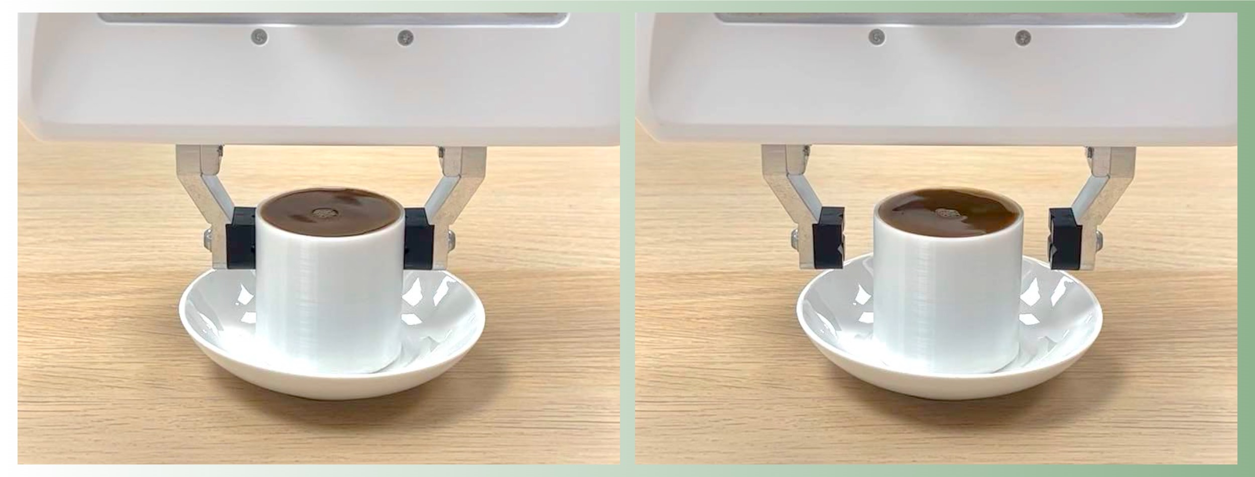
	Off by a few millimeters
(b)

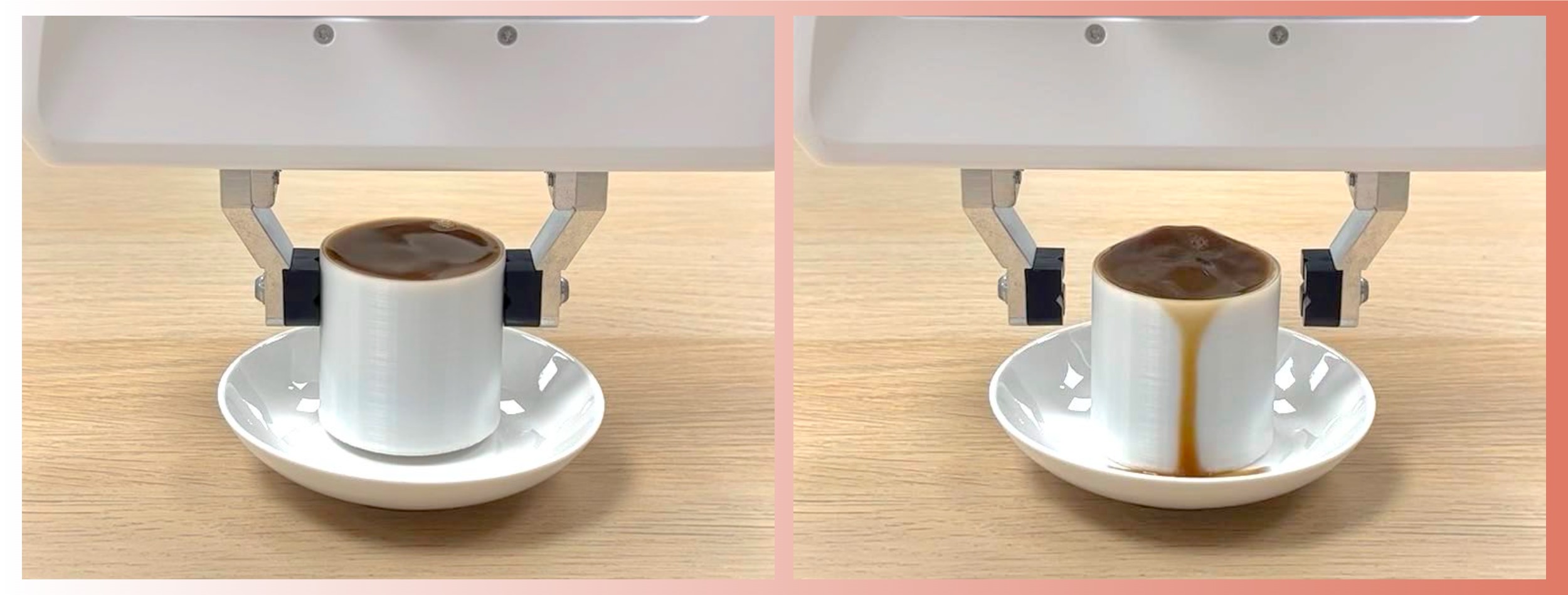
Figure 1: Placing a full cup of coffee on a saucer (left column), then releasing it (right column). (a) When the coffee cup is stably placed, i.e., the bottom surface of the cup is aligned with the top surface of the saucer, there is no spill after release. (b) If the gripper releases right after a sensed contact without proper estimation of geometric uncertainty, the coffee is spilled.

Stable placement is one instance of contact-rich manipulations, where geometric uncertainty has long been a challenge [2]; exploring stable placement therefore offers insights into this challenge. In contact-rich manipulations, objects interact through the establishment or cessation of contact, leading to hybrid dynamics where each contact configuration dictates a unique smooth dynamics. For example, the dynamics of placing a coffee cup changes upon making contact with a saucer, with these dynamics’ boundaries shaped by the objects’ geometries, such as the saucer’s shape. Because of the hybrid dynamics, contact-rich manipulations are sensitive to geometric uncertainty, where “small changes in the geometry of parts can have a significant impact on fine-motion strategies.”[3]

We propose a method for stable placement by estimating the geometric uncertainty using a general differentiable contact dynamics model. We estimate various geometric uncertainties in a unified way: applying gradients to align force sensor readings with model predictions. A novel aspect of our approach is the differentiation of contact forces with respect to geometric parameters, a capability underexplored in existing differentiable rigid-body simulators; we have prototyped this capability on top of the Jade simulator [4]. This capability allows us to use gradients to update our believed geometric parameters to be closer to the groundtruth. We verify our approach in the real world on a variety of geometric uncertainties, including in-hand pose uncertainty of the grasped object, the object’s shape uncertainty, and the environment’s shape uncertainty. The efficacy of our approach is compared to both a trigger-based heuristic policy and a policy based on particle filtering.

This paper primarily focuses on the geometric uncertainty. Other forms of uncertainty, such as sensor inaccuracies or control imprecision, are addressed through calibration.

II Related Work

II-A Robotic Stable Placement

There are various studies on robotic stable placement with haptic feedback [5, 6, 7]. However, each of these works is applicable to a particular type of geometric uncertainty defined by different assumptions: the object will be placed on a large flat surface, the initial contact between the object and the surface has to be a point contact with upward contact normal, the test cases are similar to the training data, etc. Our method applies to all geometric uncertainties describable by the general differentiable contact dynamics model, including the uncertainty in the grasped object’s in-hand pose, the object’s shape, and the environment’s shape.

II-B Manipulation Under Geometric Uncertainty

Geometric uncertainty has long been a challenge in manipulation [2]. For a particular setup, a manipulation policy can be manually crafted [5, 8, 9] or learned [10, 11, 12, 7, 13]; nevertheless, their generalizations are limited by the data diversity or the assumptions that guide the policy-crafting. For example, in a learning-based approach for stable placement [7], the object’s bottom surface and the environmental support surface are assumed to be flat and parallel. Our approach alleviates these restrictions by following the model-based approach.

Model-based methods hold promise of generalizing to different setups. For simpler tasks, a robust sequence of actions can be planned to achieve the goal under all possible variations of the uncertain geometry [14, 15, 3, 16]. Alternatively, the problem can be modeled as a partially observable Markov decision process [17, 18, 19]. However, these methods only utilize binary haptic sensor feedback (touch vs. no-touch) or simple termination conditions (e.g., y-force larger than a threshold); this limits their applicability to more complex tasks.

Many prior works estimate the uncertain geometry using data collected from manually-defined probing procedures [20, 21, 22, 23, 24, 25, 26, 27, 28, 29]. The quality of the estimation hugely depends on the design of the probing procedures.

We investigate the estimation of uncertain geometry in the context of an execution loop with rich haptic sensor feedback. A similar pipeline has been applied to a peg-insertion task with a fixed peg shape using the particle filter; however, the geometric uncertainty is limited to the environment’s shape [30]. By using a general differentiable contact dynamics model, we estimate various geometric uncertainties in a unified way: minimizing the discrepancy between the model prediction and the multi-dimensional continuous-value haptic sensor readings.

II-C Differentiable Contact Dynamics

Differentiable physical models have been shown to be useful in estimating the uncertain parameters [31, 32, 33]; the discrepancy between the model prediction and the observation is minimized using the gradients. We take a similar approach in the context of rigid-body contact dynamics.

To estimate the uncertain geometry, we need the gradients of contact forces with respect to the uncertain geometric parameters. Prior differentiable rigid-body simulators do not provide this capability [34, 35, 36, 37, 38, 39, 40, 41]. Lee et al. proposes a contact feature that is differentiable w.r.t. the object pose [29]; a differentiable contact feature is an important intermediary step, but the feature itself does not suffice to predict the contact force. We prototyped the gradients with respect to the uncertain geometric parameters on top of the Jade simulator [4].

III Problem Formulation

Given an initial guess of the uncertain geometry, our method takes the robot’s proprioception and the 6-axis force-torque (FT) sensor feedback as input; it outputs the robot action to approach the goal configuration to stably release the target object.

We assume a differentiable simulator

$$\mathbf{x}_{t+1},~{}\mathbf{y}_{{t+1}}=f(\mathbf{x}_{t},\mathbf{u}_{t};\boldsymbol{\theta}),$$ (1)

where $\mathbf{x}_{t}\in\mathrm{SE}(3)\times\mathbb{R}^{6}$ is the robot state consisting of the end-effector’s pose and twist, $\mathbf{u}_{t}\in\mathrm{SE}(3)$ is the robot action of reference pose, and $\mathbf{y}_{t}\in\mathbb{R}^{6}$ is contact wrench between the object and the environment. We always use the subscript $t$ in $(\cdot)_{t}$ to denote the timestep. The uncertain geometry is represented by the parameter $\boldsymbol{\theta}\in\mathbb{R}^{P}$, which, together with the known geometry, determines the shapes of all rigid bodies in the system, represented by triangle meshes. The dynamics function $f$ is differentiable with respect to $\mathbf{x}_{t}$, $\mathbf{u}_{t}$, and $\boldsymbol{\theta}$.

After the robot grasps the target object, we start with an initial guess $\boldsymbol{\theta}^{\text{init}}\in\mathbb{R}^{P}$ of the unknown groundtruth geometry $\boldsymbol{\theta}^{\text{gt}}\in\mathbb{R}^{P}$. We assume $\boldsymbol{\theta}^{\text{gt}}$ to be a constant.

To stably place the grasped object, the robot needs to release the object at a goal

$$\mathbf{x}^{\text{goal}}\in\mathcal{G}(\boldsymbol{\theta}^{\text{gt}})$$ (2)

determined by the unknown groundtruth $\boldsymbol{\theta}^{\text{gt}}$, where $\mathcal{G}$ maps a geometric parameter to a set of goal states.

We assume a deterministic policy

$$\mathbf{u}_{t}=\pi(\mathbf{x}_{t},\boldsymbol{\theta})$$ (3)

that takes the robot state and geometric parameter as inputs and outputs the robot action $\mathbf{u}_{t}$. When the groundtruth geometry is used, this policy drives the robot to the stable release configuration, i.e., $\lim_{t\to\infty}\mathbf{x}_{t}\in\mathcal{G}(\boldsymbol{\theta}^{\text{gt}})$ for the closed-loop dynamics $\mathbf{x}_{t+1},~{}\mathbf{y}_{t+1}=f\left(\mathbf{x}_{t},\pi(\mathbf{x}_{t},\boldsymbol{\theta}^{\text{gt}});\boldsymbol{\theta}^{\text{gt}}\right)$. This assumption comes from the insight that when there is no geometric uncertainty, stable placement is easy. In general, this policy can be implemented using motion planning methods [42, 43, 44], or learned conditioned on the groundtruth geometry [45]. In this work, we use heuristic policies that interpolate from the current state to the goal.

Our method relies on the FT sensor to measure the contact wrench between the object and the environment $\mathbf{y}^{\text{gt}}_{t}\in\mathbb{R}^{6}$ at timestep $t$. By minimizing the error between the prediction $\mathbf{y}_{t}$ and the measurement $\mathbf{y}^{\text{gt}}_{t}$, we expect the estimated geometric parameter $\hat{\boldsymbol{\theta}}$ to approach $\boldsymbol{\theta}^{\text{gt}}$, and $\pi(\mathbf{x}_{t},\hat{\boldsymbol{\theta}})$ drives the robot to the stable release configuration.

We assume uncertainties other than the geometric ones are compensated by calibration.

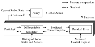
Figure 2: Our overall pipeline. At every timestep, we update the estimated geometry and plan a robot action from the estimation.

IV Approach

We start with the case of maintaining a single estimate $\hat{\boldsymbol{\theta}}_{t}$, with $\hat{\boldsymbol{\theta}}_{0}=\boldsymbol{\theta}^{\text{init}}$. At every timestep $t$, we first update the estimate from $\hat{\boldsymbol{\theta}}_{t-1}$ to $\hat{\boldsymbol{\theta}}_{t}$ using the history of the past $H+1$ timesteps, including the robot states $\mathbf{x}_{t-H:t}$, robot actions $\mathbf{u}_{t-H:t}$, and measured contact wrench $\mathbf{y}^{\text{gt}}_{t-H+1:t}$ (details are in Section IV-A). Then, we compute the robot action using the policy $\mathbf{u}_{t}=\pi\left(\mathbf{x}_{t},\hat{\boldsymbol{\theta}}_{t}\right)$. Finally, we send $\mathbf{u}_{t}$ to the robot for execution. We repeat this process for $T$ steps before the robot releases the object. During the execution, the estimate $\hat{\boldsymbol{\theta}}$ approaches $\boldsymbol{\theta}^{\text{gt}}$, and the policy drives the robot to the goal.

IV-A Estimating Uncertain Geometry

For estimation, we find the geometric parameter that minimizes the discrepancy between the prediction $\mathbf{y}_{t-H+1:t}$ and FT sensor measurement $\mathbf{y}^{\text{gt}}_{t-H+1:t}$.

Given a geometric parameter $\boldsymbol{\theta}$, we use the history data to get the predicted contact wrench

$$\mathbf{y}_{t-H+1:t}=\mathrm{Rollout}\left(\mathbf{x}_{t-H:t-1},\mathbf{u}_{t-H:t-1},\boldsymbol{\theta}\right),$$ (4)

where $\mathrm{Rollout}$ is defined by applying the simulator (1) iteratively: $\left(\cdot\right),~{}\mathbf{y}_{t^{\prime}+1}=f(x_{t^{\prime}},u_{t^{\prime}};\boldsymbol{\theta})$ for $t^{\prime}=t-H,~{}t-H+1,~{}\dots,~{}t-1$.

We define the discrepancy as the residual error between the measurement and the prediction

$$r_{t}(\boldsymbol{\theta}):=r\left(\mathbf{y}^{\text{gt}}_{t-H+1:t},~{}\mathbf{y}_{t-H+1:t}\right)\in\mathbb{R},$$ (5)

where $r\geq 0$ measures the distance between two sequences of contact wrenches; when the two sequences are identical, the residual is zero.

We find the updated geometric parameter that minimizes the residual error $\hat{\boldsymbol{\theta}}_{t}=\mathop{\mathrm{arg\,min}}_{\boldsymbol{\theta}}\;r_{t}(\boldsymbol{\theta})$ by gradient descents from $\hat{\boldsymbol{\theta}}_{t-1}$. We summarize the estimation procedure in Algorithm LABEL:alg:geometry-update.

IV-B Multiple Initialization

Gradient descents only find the local minimum and are sensitive to the initialization. To mitigate this, we keep track of a belief over multiple geometric parameters over time.

We represent the belief $\mathit{bel}_{t}$ as a set of $N$ particles, with each particle being a tuple of the value and the cost of the parameter

$$\mathit{bel}_{t}=\left\{\left\langle\hat{\boldsymbol{\theta}}_{t}^{1},~{}c_{t}^{1}\right\rangle,~{}\left\langle\hat{\boldsymbol{\theta}}_{t}^{2},~{}c_{t}^{2}\right\rangle,~{}\dots,~{}\left\langle\hat{\boldsymbol{\theta}}_{t}^{N},~{}c_{t}^{N}\right\rangle\right\},$$ (6)

where $\hat{\boldsymbol{\theta}}_{t}^{i}$ is the $i$-th parameter at timestep $t$, and $c_{t}^{i}=r_{t}\left(\hat{\boldsymbol{\theta}}_{t}^{i}\right)\geq 0$ is the cost of that parameter. To initialize the belief $\mathit{bel}_{{0}}$, we set the value $\hat{\boldsymbol{\theta}}_{0}^{i}=\boldsymbol{\theta}^{\text{init}}+\epsilon$ with $\epsilon$ sampled from a distribution of the perception noise, and the cost $c_{0}^{i}=0$, for $i=1,~{}2,~{}\dots,~{}N$.

At every timestep $t$, we first update the belief from $\mathit{bel}_{t-1}$ to $\mathit{bel}_{t}$ using the history of the past $H+1$ timesteps, including the states $\mathbf{x}_{t-H:t}$, actions $\mathbf{u}_{t-H:t}$, and measurements $\mathbf{y}^{\text{gt}}_{t-H+1:t}$ (see Algorithm LABEL:alg:belief-update). Then, we select the value of the particle with the minimum cost as the estimate $\hat{\boldsymbol{\theta}}_{t}$, and compute the robot action using the policy $\mathbf{u}_{t}=\pi(\mathbf{x}_{t},\hat{\boldsymbol{\theta}}_{t})$. Finally, we send $\mathbf{u}_{t}$ to the robot for execution. We repeat this process for $T$ steps before the robot releases the object. The overall pipeline is illustrated in Fig. 2.

V Gradients of Geometric Parameters

To differentiate the residual error in (5) with respect to the geometric parameter $\boldsymbol{\theta}$ using the chain rule, we need to have the gradient $\partial\mathbf{y}_{(\cdot)}/\partial\boldsymbol{\theta}$ from the simulator (1). However, this feature is absent in most of the existing differentiable rigid-body simulators. In this section, we describe how we implement this gradient derivation on top of the Jade simulator [4].

V-A Robot States and Actions

The robot state $\mathbf{x}_{t}=\langle\mathbf{q}_{t},\dot{\mathbf{q}}_{t}\rangle$ consists of the pose $\mathbf{q}_{t}\in\mathrm{SE}(3)$ and twist $\dot{\mathbf{q}}_{t}\in\mathbb{R}^{6}$ of the end-effector. We model the end-effector and grasped object as a floating rigid body controlled by a wrench $\boldsymbol{\tau}_{t}\in\mathbb{R}^{6}$, which is computed from the robot action $\mathbf{u}_{t}$. For example, if $\mathbf{u}_{t}$ is the reference pose of a proportional controller [46], the control wrench is given as $\boldsymbol{\tau}_{t}=\textit{ControllerGain}\cdot\mathrm{PoseError}(\mathbf{u}_{t},\mathbf{q}_{t})$.

V-B Collision-Free Forward Dynamics

We start with the simple case where no contact change occurs during each forward simulation step. We represent contacts as points between object pairs. Given $\mathbf{q}$ and $\boldsymbol{\theta}$, the collision engine detects all contact features, each as a tuple with respect to objects $A$ and $B$

$$\left\langle\mathbf{p}^{A}(\mathbf{q};\boldsymbol{\theta}),~{}\mathbf{p}^{B}(\mathbf{q};\boldsymbol{\theta}),~{}\mathbf{v}^{A},~{}\mathbf{v}^{B},~{}\mathbf{n}(\mathbf{q};\boldsymbol{\theta})\right\rangle,$$ (7)

where $\mathbf{p}^{A},\mathbf{p}^{B}\in\mathbb{R}^{3}$ are the coordinates of contact points on objects $A$ and $B$, $\mathbf{v}^{A},\mathbf{v}^{B}\in\mathbb{R}^{3}$ are the velocities of contact points, and $\mathbf{n}\in\mathrm{S}(3)$ is the unit normal vector of contact surface pointing from object $A$ to object $B$. When the collision happens, we have $\mathbf{p}^{A}=\mathbf{p}^{B}$.

Given the detected $C$ contact features (7), the simulator predicts the position $\mathbf{q}^{\prime}$, velocity $\dot{\mathbf{q}}^{\prime}$ and contact impulse $\boldsymbol{\lambda}\in\mathbb{R}^{3C}$ after applying the control force $\boldsymbol{\tau}$ for the time duration $\Delta$

$$\mathbf{q}^{\prime},~{}\dot{\mathbf{q}}^{\prime},~{}\boldsymbol{\lambda}=\operatorname{FD}\left(\mathbf{q},\dot{\mathbf{q}},\boldsymbol{\tau},\Delta;\boldsymbol{\theta}\right)$$ (8)

under the assumption that the contact features do not change during $\Delta$, i.e., there is no collision during $\Delta$. Let $\Delta_{0}$ be the duration between two timesteps $t$ and $t+1$, we have $\mathbf{q}_{t+1},\dot{\mathbf{q}}_{t+1},\boldsymbol{\lambda}_{t}=\operatorname{FD}(\mathbf{q}_{t},\dot{\mathbf{q}}_{t},\boldsymbol{\tau}_{t},\Delta_{0};\boldsymbol{\theta})$, and the predicted contact wrench is $\mathbf{y}_{t+1}=\mathbf{J}^{\top}(\mathbf{q}_{t};\boldsymbol{\theta})\boldsymbol{\lambda}_{t}$, where $\mathbf{J}\in\mathbb{R}^{6\times 3C}$ is the contact Jacobian that depends on (7).

We solve for $\boldsymbol{\lambda}$ in (8) via a linear complementarity problem $\boldsymbol{\lambda}=\mathrm{LCP}\left(\mathbf{A},\mathbf{b}\right)$: finding $\langle\boldsymbol{\lambda},~{}\mathbf{a}\rangle$ such that $\boldsymbol{\lambda}\geq 0$, $\mathbf{a}\geq 0$, $\boldsymbol{\lambda}^{\top}\mathbf{a}=0$, and $\mathbf{a}=\mathbf{A}\boldsymbol{\lambda}+\mathbf{b}$. Here we highlight that the $\mathrm{LCP}$ parameters $\mathbf{A}=\mathbf{A}(\mathbf{J})$ and $\mathbf{b}=\mathbf{b}(\mathbf{J},\Delta)$ depend on $\mathbf{J}$ and $\Delta$.

However, the assumption of no contact change during the forward simulation step (8) rarely holds. We alleviate this assumption in the next subsection.

V-C Collision Between Two Timesteps

If there is a collision between timesteps $t$ and  $t+1$ that changes the contact features (7), we can detect the exact time-of-impact $\mathit{toi}$ when two rigid bodies collide. The general forward dynamics

$$\mathbf{q}_{t+1},~{}\dot{\mathbf{q}}_{t+1}=\operatorname{FD}_{\text{full}}\left(\mathbf{q}_{t},\dot{\mathbf{q}}_{t},\boldsymbol{\tau}_{t},\Delta_{0};\boldsymbol{\theta}\right)$$ (9)

might involve multiple calls of collision-free forward dynamics [4]. In the case of 2 calls, we have

$$\mathbf{q}_{t+\mathit{toi}},~{}\dot{\mathbf{q}}_{t+\mathit{toi}},~{}\boldsymbol{\lambda}_{t} =\operatorname{FD}\left(\mathbf{q}_{t},\dot{\mathbf{q}}_{t},\boldsymbol{\tau}_{t},\mathit{toi};\boldsymbol{\theta}\right),$$

$$\mathbf{q}_{t+1},~{}\dot{\mathbf{q}}_{t+1},~{}\boldsymbol{\lambda}_{t+\mathit{toi}} =\operatorname{FD}\left(\mathbf{q}_{t+\mathit{toi}},\dot{\mathbf{q}}_{t+\mathit{toi}},\boldsymbol{\tau}_{t},\Delta_{0}-\mathit{toi};\boldsymbol{\theta}\right).$$

We have so far defined the forward dynamics of the simulator (1). Prior works [39, 4] have implemented the gradients $\partial\operatorname{FD}/\partial\mathbf{q}$, $\partial\operatorname{FD}/\partial\dot{\mathbf{q}}$, $\partial\operatorname{FD}/\partial\boldsymbol{\tau}$, and $\partial\operatorname{FD}/\partial\Delta$. However, our method needs $\partial\mathbf{y}_{(\cdot)}/\partial\boldsymbol{\theta}$ from the simulator (1). We elaborate how we obtain it in the next subsection.

V-D Differentiating Wrench wrt Geometric Parameters

Since in our problem setup, $\mathbf{q}_{t}$ is the pose of the robot’s end-effector, the contact wrench impulse between the grasped object and the environment is given as

$$\mathbf{y}_{t+1}=\left\{\begin{array}[]{ll}\mathbf{J}^{\top}_{t+\mathit{toi}}\boldsymbol{\lambda}_{t+\mathit{toi}}+\mathbf{J}^{\top}_{t}\boldsymbol{\lambda}_{t}&\text{ collision,}\\ \mathbf{J}^{\top}_{t}\boldsymbol{\lambda}_{t}&\text{ no collision.}\end{array}\right.$$ (10)

By applying the chain rule, the gradient of the geometric parameter $\partial\mathbf{y}_{t+1}/\partial\boldsymbol{\theta}$ involves the differentiation of contact impulses $\partial\boldsymbol{\lambda}_{(\cdot)}/\partial\boldsymbol{\theta}$ and the Jacobian $\partial\mathbf{J}^{\top}_{(\cdot)}/\partial\boldsymbol{\theta}$, where $\partial\boldsymbol{\lambda}_{(\cdot)}/\partial\boldsymbol{\theta}$ involves $\partial\mathbf{J}^{\top}_{(\cdot)}/\partial\boldsymbol{\theta}$, $\partial\mathbf{J}_{(\cdot)}/\partial\boldsymbol{\theta}$ and $\partial\mathit{toi}/\partial\boldsymbol{\theta}$.

To derive $\partial\mathit{toi}/\partial\boldsymbol{\theta}$, we consider the dynamics at timestep $t+\mathit{toi}$ as discussed in [4]. Suppose a tiny geometry variant $\delta\boldsymbol{\theta}$ causes coordinate variants $\delta\mathbf{p}_{1},\delta\mathbf{p}_{2}$ and makes the contact points separate along the normal direction, it’ll take

$$\delta\mathit{toi}=\frac{(\delta\mathbf{p}^{B}-\delta\mathbf{p}^{A})\cdot\mathbf{n}}{(\mathbf{v}^{B}-\mathbf{v}^{A})\cdot\mathbf{n}}$$

longer for them to collide and vice versa. Denote $v_{n}=(\mathbf{v}^{B}-\mathbf{v}^{A})\cdot\mathbf{n}$ as the relative normal velocity. We have

$$\frac{\partial\mathit{toi}}{\partial\boldsymbol{\theta}}=\left.\frac{\mathbf{n}^{\top}}{v_{n}}\left(\frac{\partial\mathbf{p}^{B}}{\partial\boldsymbol{\theta}}-\frac{\partial\mathbf{p}^{A}}{\partial\boldsymbol{\theta}}\right)\right|_{\mathbf{q}=\mathbf{q}_{t+\mathit{toi}}}.$$ (11)

When there is no collision, we treat $\Delta$ as a constant in (9).

The gradients of Jacobian $\partial\mathbf{J}^{\top}/\partial\boldsymbol{\theta}$ and $\partial\mathbf{J}/\partial\boldsymbol{\theta}$ are always calculated in the context of $\partial\left(\mathbf{J}^{\top}\mathbf{z}\right)/\partial\boldsymbol{\theta}$ and $\partial\left(\mathbf{J}\mathbf{z}^{\prime}\right)/\partial\boldsymbol{\theta}$, with $\mathbf{z}$ and $\mathbf{z}^{\prime}$ being arbitrary constant vectors. In our setting, the $i$-th column $\mathbf{J}^{{i}^{\top}}=\left[(\mathbf{n}^{i}\times\mathbf{p}^{i})^{\top}~{}\mathbf{n}^{{i}^{\top}}\right]^{\top}$ of $\mathbf{J}^{\top}$ is defined by the location $\mathbf{p}^{i}$ and normal $\mathbf{n}^{i}$ of the corresponding contact feature (7). Then, $\mathbf{J}^{\top}\mathbf{z}=\sum_{i}\mathbf{J}^{{i}^{\top}}z^{i}$ and

$$\frac{\partial\left(\mathbf{J}^{\top}\mathbf{z}\right)}{\partial\boldsymbol{\theta}}=\sum_{i}\left[\begin{array}[]{c}\left(\partial\mathbf{n}^{i}/\partial\boldsymbol{\theta}\right)\times\mathbf{p}^{i}+\mathbf{n}^{i}\times\left(\partial\mathbf{p}^{i}/\partial\boldsymbol{\theta}\right)\\ \left(\partial\mathbf{n}^{i}/\partial\boldsymbol{\theta}\right)\end{array}\right]z^{i},$$

where $z^{i}\in\mathbb{R}$ is the $i$-th element of $\mathbf{z}$. We derive $\partial\left(\mathbf{J}\mathbf{z}^{\prime}\right)/\partial\boldsymbol{\theta}$ in a similar manner.

For our current prototype, the user needs to specify the functions to calculate the derivatives of the contact features $\mathbf{p}_{(\cdot)}$ and $\mathbf{n}_{(\cdot)}$ with respect to the geometric parameter $\boldsymbol{\theta}$ for each URDF file. We expect future simulators to provide automatic routines in the collision engine.

VI Experiment

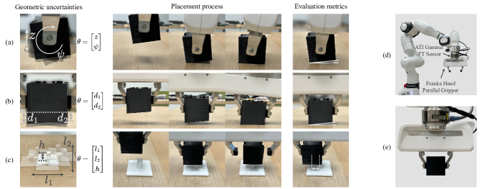
Figure 3: Experimental setups. (a)-(c) Visualization of the task setups for (a) pose, (b) shape and (c) env: the left column shows the unknown geometric parameters, the middle columns show an ideal placement process, and the right column visualizes the distance to goal when releasing. (d) The ATI Gamma sensor and Franka Hand mounted on a Franka Research 3 arm. (e) The robot’s grasp on a cube when there is no geometric uncertainty.

VI-A Tasks

We evaluate our proposed method on 3 tasks with different kinds of geometric uncertainty: pose, shape, and env. The geometric uncertainty and placement processes of the 3 tasks are illustrated in Fig. 3.

In pose, the robot needs to stably place a cube on the table surface. The goal set $\mathcal{G}$ in (2) is defined by all configurations that the bottom surface of the cube is aligned with the table surface. Nominally, the cube’s bottom surface is parallel to the table surface, and the robot grasps it at its center (Fig. 3(e)); in reality, the object’s in-hand pose has uncertainty, represented as a translation $z$ and a rotation $\psi$.

shape has the same task requirement, goal set, and nominal geometry as pose, and a different kind of geometric uncertainty. The left and right walls have uncertain heights, defined by the deviations from the nominal values $d_{1}$ and $d_{2}$.

In env, the robot needs to place the cube on a pillar, whose top square surface is parallel to the table surface; the square’s side length is 15 mm. The goal set $\mathcal{G}$ in (2) contains a single configuration that the center of the object’s bottom surface coincides with that of the pillar’s top surface. The horizontal locations and height of the pillar have uncertainty, represented as the deviations from the nominal values $l_{1}$, $l_{2}$ and $h$.

In all tasks, the nominal values of the uncertain geometry are $0$, and are used as the initial guess $\boldsymbol{\theta}^{\text{init}}=0$. Each task has 10 test cases of different groundtruth geometric parameters $\boldsymbol{\theta}^{\text{gt}}\neq\boldsymbol{\theta}^{\text{init}}$. The groundtruth geometric parameters $\boldsymbol{\theta}^{\text{gt}}$ are obtained from manual calibration and CAD models of the 3D-printed cubes/pillar. We set the duration $T=50$ and the history $H=5$ timesteps for all tasks. At the initial robot configuration, the gripper is $10$ cm above a nominal goal defined by the nominal geometric parameter $\mathcal{G}(\boldsymbol{\theta}^{\text{init}})$.

VI-B Setup

We carry out the experiments on a Franka Research 3 (FR3) arm. We mount an ATI Gamma FT sensor on the flange of the FR3 arm, and mount the Franka Hand parallel gripper to the FT sensor. See Fig. 3(d).

Since our tasks are quasi-static and the inertial effect is negligible, we assume the FT sensor measures the contact wrench between the object and the environment. In general, one can use the generalized momentum observer to estimate the object-environment wrench [47].

We assume the operational-space dynamics [48] and impedance control [49, 50] for the system (1), with $\mathbf{u}_{t}$ being the reference equilibrium pose. The generalized bias forces are compensated. Since during the 3 placement tasks, the robot moves in a small space, we approximate the operational-space inertia as a constant matrix.

We implement the policy (3) as a heuristic that interpolates from the current robot state $\mathbf{x}_{t}$ to the closest goal state in $\mathcal{G}(\boldsymbol{\theta})$. We have verified that when $\boldsymbol{\theta}=\boldsymbol{\theta}^{\text{gt}}$, this policy indeed drives the robot to a goal $\mathbf{x}^{\text{goal}}\in\mathcal{G}(\boldsymbol{\theta}^{\text{gt}})$.

The differentiable simulation does not run in real-time; since our tasks are quasi-static, we pause the estimation and keep the same reference pose when waiting for the next robot action. The average computation time per action is $3.36$ seconds. We expect a better-implemented differentiable contact simulation to achieve real-time computation. Our prototype needs to reload the URDF description every time the geometric parameter is updated (Line LABEL:line:geometry-update in Algorithm LABEL:alg:geometry-update). Additionally, the speed of the differentiable simulation could be significantly improved. For instance, our prototype uses PyTorch’s auto-differentiation interface, causing data to be passed between Python and C++ at each simulation step [51, 39, 4]. Differentiable contact simulation has already achieved real-time computation in locomotion planning [44]; we expect real-time computation to be achievable in estimating geometric uncertainty.

VI-C Baselines

Granted that we can design an optimal policy for a particular task [52], here we consider two baselines that are applicable in all scenarios. The first baseline PF replaces our gradient-based estimator by a particle filter [53]. Similar to the prior works [54, 27], we add a small Gaussian noise during the prediction update, and the unnormalized weight of the $i$-th particle is given as

$$\operatorname{Weight}\left(\hat{\boldsymbol{\theta}}_{t}^{i}\right)=\exp\left(-\beta c_{t}^{i}\right)$$ (12)

with $\beta$ being a positive constant. We implement the low variance sampler as described in [53]. The PF implementation is summarized in Algorithm LABEL:alg:belief-update-pf.

The second baseline is a trigger-based heuristic policy. The robot moves downwards until the measured contact wrench is larger than a threshold. This baseline demonstrates the performance of a compliant controller that does not explicitly reason about the geometric uncertainties. When there is no geometric uncertainty $\boldsymbol{\theta}^{\text{init}}=\boldsymbol{\theta}^{\text{gt}}$ or there is only uncertainty in heights, this heuristic policy is sufficient to reach a goal in $\mathcal{G}(\boldsymbol{\theta}^{\text{gt}})$ for all tasks.

We use $N=50$ particles for PF, and $N=10$ particles in our method. This ensures that the two methods have the same number of total rollouts in each timestep.

VI-D Evaluation Metric

We measure the distance to goal errors when the robot releases the object. In our particular tasks, instead of measuring the distance between poses [55, 56], we apply simplifications to have consistent physical dimensions. For pose and shape, since in all test cases for all methods, the cube touches the table surface, we reduce the distance to goal error to the angle between the cube’s bottom surface and the table surface. For env, we measure the horizontal distance between the centers of the cube and the pillar. The evaluation metrics for the 3 tasks are illustrated in Fig. 3.

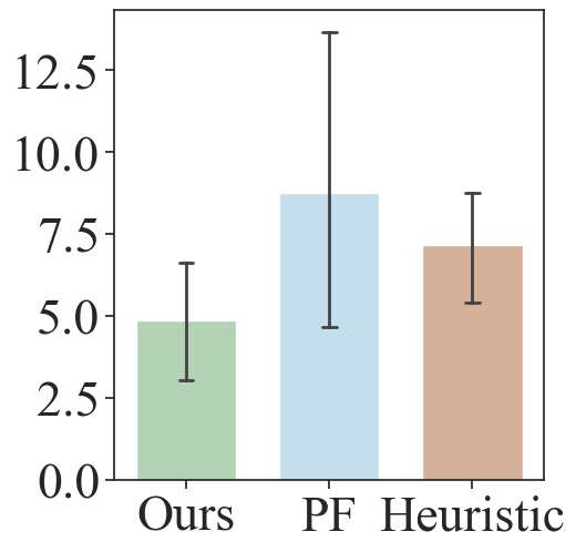
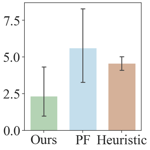
Angle Error [deg]			Dist. Error [mm]
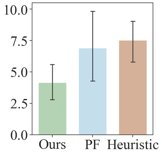
	(a)	(b)		(c)

Figure 4: Our method has smaller distance to the goal errors when the robot releases. We plot the means and 95% confidence intervals over 10 test cases. For (a) pose and (b) shape, the errors are equivalent to angle errors. For (c) env, the errors are equivalent to distance errors.

	Ours, case #8	PF, case #8	PF, case #7
$d_{{1}}$ [mm]
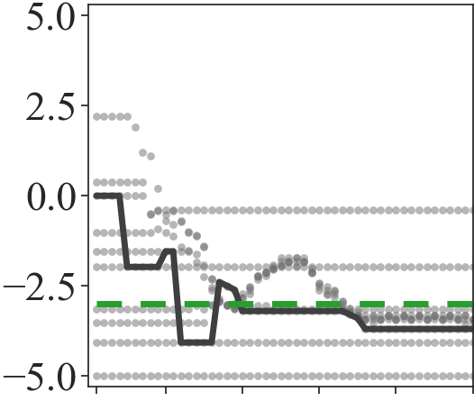
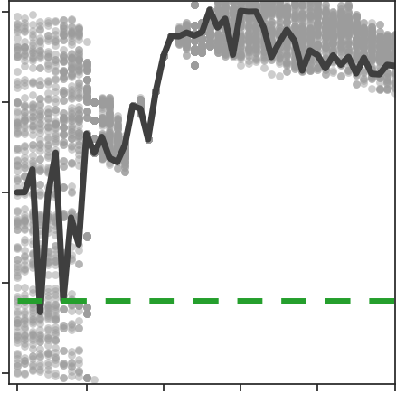
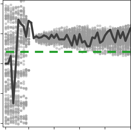
$d_{{2}}$ [mm]
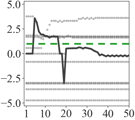
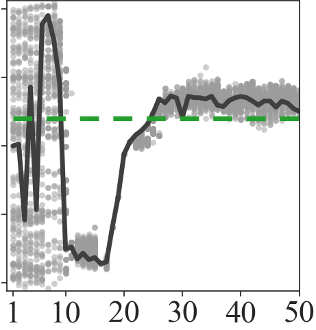
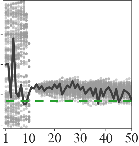
		Timestep
	(a)	(b)	(c)

Figure 5: PF might suffer from “particle starvation”. We plot estimation over time from 2 test cases of the shape task. In the same test case, ours (a) has good estimate, while PF (b) diverges on $d_{1}$ due to “particle starvation.” (c) In a different test case, PF maintains good estimate.

	Lateral	Height	Depth
Location [mm]
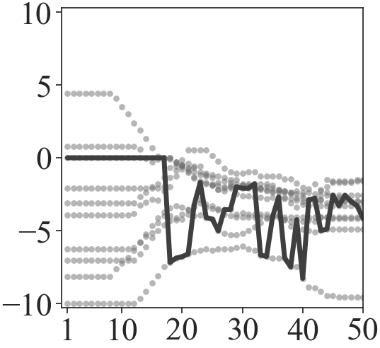
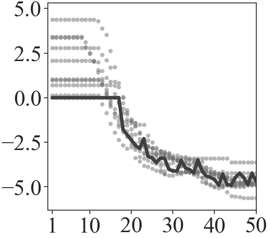
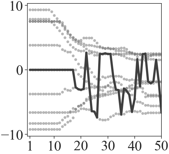
		Timestep

Figure 6: We deployed our method to place a full cup of coffee on a saucer of uncertain location. We plot the estimation of the saucer’s location over time. The variance of the estimation reduces over time.

VI-E Results

Fig. 4 shows the errors over the 10 test cases for the 3 tasks. Our proposed method achieves smaller average errors than the PF and heuristic baselines. Interestingly, PF baseline does not always outperform the heuristic baseline on average, even though it has better best performance. When PF has bad performance, we observe “particle starvation”, where most particles “collapse” to a small range of wrong values [57]. Fig. 5(a)-(b) show the eighth test case from shape. In Fig. 5(b), PF’s estimate on $d_{1}$ collapsed to the wrong value, while in Fig. 5(a) our gradient-based estimator maintains an estimate closer to the groundtruth. The particle starvation does not always happen. Fig. 5(c) shows PF’s estimate over time in the seventh test case from shape, where PF’s estimate is close to the groundtruth.

VI-F Placing a Full Cup of Coffee

Lastly, we deploy our method to place a full cup of coffee on a saucer. We relax a few assumptions from Section III. We approximate the cup of coffee with a solid rigid cylinder. In addition, we only have an approximate mesh of the saucer. The setup is depicted in Fig. 1. We represent the geometric uncertainty $\boldsymbol{\theta}$ as the 3-dimensional location of the saucer. Our method successfully placed a full cup of coffee on the saucer without spilling. We plot $\hat{\boldsymbol{\theta}}$ over time in Fig. 6.

VII Conclusion and Discussion

We have presented a pipeline for stable placement under geometric uncertainty using the differentiable contact dynamics. We prototype the gradients with respect to the geometric parameters on top of a differentiable simulator. By using the gradient to minimize the discrepancy between the measurements and the predictions, we achieve better results than the gradient-free particle filter baseline. Nevertheless, in this work, we only consider geometric uncertainties, and our implementation does not achieve real-time speed. We expect these limitations to be addressed in the future.

References

- [1] Intel, “Intel® RealSenseTM Product Family D400 Series Datasheet,” 2020.
- [2] A. Rodriguez, “The unstable queen: Uncertainty, mechanics, and tactile feedback,” Science Robotics, vol. 6, no. 54, 2021.
- [3] T. Lozano-Pérez, M. T. Mason, and R. H. Taylor, “Automatic synthesis of fine-motion strategies for robots,” Int. J. Robotics Research, vol. 3, no. 1, pp. 3–24, 1984.
- [4] G. Yang, S. Luo, Y. Feng, Z. Sun, C. Tie, and L. Shao, “Jade: A Differentiable Physics Engine for Articulated Rigid Bodies with Intersection-Free Frictional Contact,” in IEEE Int. Conf. on Robotics & Automation, 2024.
- [5] J. M. Romano, K. Hsiao, G. Niemeyer, S. Chitta, and K. J. Kuchenbecker, “Human-Inspired Robotic Grasp Control With Tactile Sensing,” IEEE Trans. on Robotics, vol. 27, no. 6, pp. 1067–1079, 2011.
- [6] S. Kim, D. K. Jha, D. Romeres, P. Patre, and A. Rodriguez, “Simultaneous Tactile Estimation and Control of Extrinsic Contact,” in IEEE Int. Conf. on Robotics & Automation, 2023.
- [7] K. Ota, D. K. Jha, K. M. Jatavallabhula, A. Kanezaki, and J. B. Tenenbaum, “Tactile Estimation of Extrinsic Contact Patch for Stable Placement,” in IEEE Int. Conf. on Robotics & Automation, 2024.
- [8] J. Stückler and S. Behnke, “Adaptive tool-use strategies for anthropomorphic service robots,” in IEEE-RAS Int. Conf. on Humanoid Robots, 2014.
- [9] F. Suárez-Ruiz, X. Zhou, and Q.-C. Pham, “Can robots assemble an ikea chair?,” Science Robotics, vol. 3, no. 17, 2018.
- [10] T. Inoue, G. De Magistris, A. Munawar, T. Yokoya, and R. Tachibana, “Deep Reinforcement Learning for High Precision Assembly Tasks,” in IEEE/RSJ Int. Conf. on Intelligent Robots & Systems, 2017.
- [11] T. Johannink, S. Bahl, A. Nair, J. Luo, A. Kumar, M. Loskyll, J. A. Ojea, E. Solowjow, and S. Levine, “Residual Reinforcement Learning for Robot Control,” in IEEE Int. Conf. on Robotics & Automation, 2019.
- [12] S. Jin, X. Zhu, C. Wang, and M. Tomizuka, “Contact Pose Identification for Peg-in-Hole Assembly under Uncertainties,” in American Control Conf., 2021.
- [13] X. Zhang, M. Tomizuka, and H. Li, “Bridging the Sim-to-Real Gap with Dynamic Compliance Tuning for Industrial Insertion,” in IEEE Int. Conf. on Robotics & Automation, 2024.
- [14] M. Erdmann and M. Mason, “An exploration of sensorless manipulation,” IEEE Journal on Robotics and Automation, vol. 4, no. 4, pp. 369–379, 1988.
- [15] K. Y. Goldberg, “Orienting polygonal parts without sensors,” Algorithmica, vol. 10, no. 2-4, pp. 210–225, 1993.
- [16] F. Wirnshofer, P. S. Schmitt, W. Feiten, G. v. Wichert, and W. Burgard, “Robust, Compliant Assembly via Optimal Belief Space Planning,” in IEEE Int. Conf. on Robotics & Automation, 2018.
- [17] K. Hsiao, L. P. Kaelbling, and T. Lozano-Pérez, “Grasping POMDPs,” in IEEE Int. Conf. on Robotics & Automation, 2007.
- [18] M. C. Koval, N. S. Pollard, and S. S. Srinivasa, “Pre- and post-contact policy decomposition for planar contact manipulation under uncertainty,” Int. J. Robotics Research, vol. 35, no. 1-3, pp. 244–264, 2016.
- [19] B. Saund, S. Choudhury, S. Srinivasa, and D. Berenson, “The blindfolded traveler’s problem: A search framework for motion planning with contact estimates,” Int. J. Robotics Research, vol. 42, no. 4-5, pp. 289–309, 2023.
- [20] S. Chhatpar and M. Branicky, “Localization for Robotic Assemblies Using Probing and Particle Filtering,” in IEEE/ASME Int. Conf. on Advanced Intelligent Mechatronics., 2005.
- [21] Y. Taguchi, T. K. Marks, and H. Okuda, “Rao-Blackwellized Particle Filtering for Probing-Based 6-DOF Localization in Robotic Assembly,” in IEEE Int. Conf. on Robotics & Automation, 2010.
- [22] F. von Drigalski, K. Hayashi, Y. Huang, R. Yonetani, M. Hamaya, K. Tanaka, and Y. Ijiri, “Precise Multi-Modal In-Hand Pose Estimation using Low-Precision Sensors for Robotic Assembly,” in IEEE Int. Conf. on Robotics & Automation, 2021.
- [23] B. Saund and D. Berenson, “CLASP: Constrained Latent Shape Projection for Refining Object Shape from Robot Contact,” in Conference on Robot Learning, 2022.
- [24] D. Ma, S. Dong, and A. Rodriguez, “Extrinsic Contact Sensing with Relative-Motion Tracking from Distributed Tactile Measurements,” in IEEE Int. Conf. on Robotics & Automation, 2021.
- [25] K. Gadeyne, T. Lefebvre, and H. Bruyninckx, “Bayesian hybrid model-state estimation applied to simultaneous contact formation recognition and geometrical parameter estimation,” Int. J. Robotics Research, vol. 24, no. 8, pp. 615–630, 2005.
- [26] K. Hertkorn, M. A. Roa, C. Preusche, C. Borst, and G. Hirzinger, “Identification of Contact Formations: Resolving Ambiguous Force Torque Information,” in IEEE Int. Conf. on Robotics & Automation, 2012.
- [27] A. Sipos and N. Fazeli, “Simultaneous Contact Location and Object Pose Estimation Using Proprioceptive Tactile Feedback,” in IEEE/RSJ Int. Conf. on Intelligent Robots & Systems, 2022.
- [28] A. Sipos and N. Fazeli, “MultiSCOPE: Disambiguating In-Hand Object Poses with Proprioception and Tactile Feedback,” in Robotics: Science & Systems, 2023.
- [29] J. Lee, M. Lee, and D. Lee, “Uncertain Pose Estimation during Contact Tasks using Differentiable Contact Features,” in Robotics: Science & Systems, 2023.
- [30] U. Thomas, S. Molkenstruck, R. Iser, and F. M. Wahl, “Multi Sensor Fusion in Robot Assembly Using Particle Filters,” in IEEE Int. Conf. on Robotics & Automation, 2007.
- [31] Y. Li, J. Wu, R. Tedrake, J. B. Tenenbaum, and A. Torralba, “Learning Particle Dynamics for Manipulating Rigid Bodies, Deformable Objects, and Fluids,” in Int. Conf. on Learning Representations, 2019.
- [32] P. Mitrano, A. LaGrassa, O. Kroemer, and D. Berenson, “Focused Adaptation of Dynamics Models for Deformable Object Manipulation,” in IEEE Int. Conf. on Robotics & Automation, 2023.
- [33] S. Le Cleac’h, H.-X. Yu, M. Guo, T. Howell, R. Gao, J. Wu, Z. Manchester, and M. Schwager, “Differentiable Physics Simulation of Dynamics-Augmented Neural Objects,” IEEE Robotics & Automation Letters, vol. 8, no. 5, pp. 2780–2787, 2023.
- [34] F. de Avila Belbute-Peres, K. Smith, K. Allen, J. Tenenbaum, and J. Z. Kolter, “End-to-End Differentiable Physics for Learning and Control,” in Advances in Neural Information Processing Systems, 2018.
- [35] E. Heiden, D. Millard, E. Coumans, Y. Sheng, and G. S. Sukhatme, “NeuralSim: Augmenting Differentiable Simulators with Neural Networks,” in IEEE Int. Conf. on Robotics & Automation, 2021.
- [36] J. Degrave, M. Hermans, J. Dambre, et al., “A differentiable physics engine for deep learning in robotics,” Frontiers in neurorobotics, p. 6, 2019.
- [37] Y. Qiao, J. Liang, V. Koltun, and M. C. Lin, “Scalable Differentiable Physics for Learning and Control,” in Int. Conf. on Machine Learning, 2020.
- [38] Y. Qiao, J. Liang, V. Koltun, and M. C. Lin, “Efficient Differentiable Dimulation of Articulated Bodies,” in Int. Conf. on Machine Learning, 2021.
- [39] K. Werling, D. Omens, J. Lee, I. Exarchos, and C. K. Liu, “Fast and Feature-Complete Differentiable Physics Engine for Articulated Rigid Bodies with Contact Constraints,” in Robotics: Science & Systems, 2021.
- [40] M. Geilinger, D. Hahn, J. Zehnder, M. Bächer, B. Thomaszewski, and S. Coros, “ADD: Analytically Differentiable Dynamics for Multi-Body Systems with Frictional Contact,” ACM Trans. on Graphics, vol. 39, no. 6, pp. 1–15, 2020.
- [41] T. A. Howell, S. L. Cleac’h, J. Z. Kolter, M. Schwager, and Z. Manchester, “Dojo: A differentiable simulator for robotics,” arXiv preprint arXiv:2203.00806, 2022.
- [42] M. Toussaint, K. Allen, K. Smith, and J. Tenenbaum, “Differentiable Physics and Stable Modes for Tool-Use and Manipulation Planning,” in Robotics: Science & Systems, 2018.
- [43] T. Pang, H. J. T. Suh, L. Yang, and R. Tedrake, “Global Planning for Contact-Rich Manipulation via Local Smoothing of Quasi-Dynamic Contact Models,” IEEE Trans. on Robotics, pp. 1–21, 2023.
- [44] S. Le Cleac’h, T. A. Howell, S. Yang, C.-Y. Lee, J. Zhang, A. Bishop, M. Schwager, and Z. Manchester, “Fast Contact-Implicit Model Predictive Control,” IEEE Trans. on Robotics, vol. 40, pp. 1617–1629, 2024.
- [45] A. Kumar, Z. Fu, D. Pathak, and J. Malik, “RMA: Rapid Motor Adaptation for Legged Robots,” in Robotics: Science & Systems, 2021.
- [46] K. J. Åström and R. M. Murray, Feedback Systems. 2010.
- [47] A. de Luca and R. Mattone, “Sensorless Robot Collision Detection and Hybrid Force/Motion Control,” in IEEE Int. Conf. on Robotics & Automation, 2005.
- [48] O. Khatib, “A unified approach for motion and force control of robot manipulators: The operational space formulation,” IEEE Journal of Robotics and Automation, vol. 3, no. 1, pp. 43–53, 1987.
- [49] N. Hogan, “Impedance control: An approach to manipulation. I - theory. II - implementation. III - applications,” ASME Journal of Dynamic Systems, Measurement, and Control, pp. 1–24, 1985.
- [50] N. Hogan and S. P. Buerger, “Impedance and interaction control 19.1,” Robotics and automation handbook, pp. 19–1, 2005.
- [51] A. Bilogur, “PyTorch Training Performance Guide - Eager versus graph execution.” https://residentmario.github.io/pytorch-training-performance-guide/jit.html#eager-versus-graph-execution, 2021.
- [52] M. Khansari, E. Klingbeil, and O. Khatib, “Adaptive human-inspired compliant contact primitives to perform surface–surface contact under uncertainty,” Int. J. Robotics Research, vol. 35, no. 13, pp. 1651–1675, 2016.
- [53] S. Thrun, W. Burgard, and D. Fox, Probabilistic Robotics. 2005.
- [54] L. Manuelli and R. Tedrake, “Localizing External Contact Using Proprioceptive Sensors: The Contact Particle Filter,” in IEEE/RSJ Int. Conf. on Intelligent Robots & Systems, 2016.
- [55] J. Sola, J. Deray, and D. Atchuthan, “A micro Lie theory for state estimation in robotics,” arXiv preprint arXiv:1812.01537, 2018.
- [56] K. M. Lynch and F. C. Park, Modern Robotics. 2017.
- [57] M. C. Koval, N. S. Pollard, and S. S. Srinivasa, “Pose estimation for planar contact manipulation with manifold particle filters,” Int. J. Robotics Research, vol. 34, no. 7, pp. 922–945, 2015.