QuForge: A Library for Qudits Simulation

Abstract

Quantum computing with qudits, an extension of qubits to multiple levels, is a research field less mature than qubit-based quantum computing. However, qudits can offer some advantages over qubits, by representing information with fewer separated components. In this article, we present QuForge, a Python-based library designed to simulate quantum circuits with qudits. This library provides the necessary quantum gates for implementing quantum algorithms, tailored to any chosen qudit dimension. Built on top of differentiable frameworks, QuForge supports execution on accelerating devices such as GPUs and TPUs, significantly speeding up simulations. It also supports sparse operations, leading to a reduction in memory consumption compared to other libraries. Additionally, by constructing quantum circuits as differentiable graphs, QuForge facilitates the implementation of quantum machine learning algorithms, enhancing the capabilities and flexibility of quantum computing research.

I Introduction

Differentiable programming frameworks, including but not limited to PyTorch [1] and JAX [2], offer a robust infrastructure for the construction of algorithms composed of differentiable components [3]. The inherent differentiability of these frameworks enables the training of parameterized programs through data-driven methodologies. This capability is pivotal for optimizing program parameters to enhance performance in tasks such as machine learning and deep learning [4].

Moreover, these differentiable programming frameworks are designed with a high degree of versatility, allowing for seamless execution across a diverse spectrum of hardware platforms. This adaptability enables the execution of complex computational tasks on a variety of computing devices, ranging from conventional CPUs to specialized hardware like GPUs and TPUs [5]. Such flexibility not only accelerates execution times but also broadens the applicability of differentiable programming in addressing a wide range of scientific and engineering challenges.

In the realm of quantum computing, research and engineering efforts predominantly focus on systems based on quantum bits, or qubits [6]. Distinguished by their ability to exist in a superposition of two states, labeled 0 and 1, qubits leverage this property of quantum mechanics, alongside with quantum entanglement, to achieve the desired computational outcomes in the majority of quantum algorithms. Expanding beyond this binary framework, the concept of qubits extends to qudits [7], or $d$-dimensional quantum systems, which possess the capacity of being in a quantum superposition of more than two states.

By transcending the binary constraint of qubits, qudits facilitate a denser encoding of information, enabling the representation and processing of a larger volume of data within the same quantum system [8, 9]. This enhanced capacity for information storage and manipulation significantly improves the efficiency and scalability of quantum algorithms, allowing for the tackling of more complex problems with fewer quantum resources.

Furthermore, the expanded state space of qudits opens new avenues for exploring novel quantum phenomena and interactions, potentially catalyzing breakthroughs in quantum simulation [10, 11], cryptography [12], and communication [13]. The capacity to engage with higher-dimensional quantum systems may also lead to more robust error correction schemes and quantum gate operations [14], which are crucial for the development of practical, fault-tolerant quantum computers.

The development of a differentiable high-level library for qudit simulation, capable of execution across various hardware platforms, represents an advancement in the field of quantum computing. Such a library could democratize access to advanced quantum simulations, enabling researchers and engineers to explore the potential of qudits and potentially accelerate the pace of innovation in quantum technologies.

In this article, we introduce a Python-based library specifically designed for qudit simulation, adeptly meeting the critical requirements for differentiability and execution across multiple hardware platforms. A key innovation of this library is its strategic use of sparse operations [15], significantly enhancing scalability. By leveraging sparse matrix operations, the library markedly reduces the computational resources required for simulating systems with a large number of qudits, compared to conventional approaches that rely on dense matrix operations.

The sequence of this article is organized as follows. In Sec. II we discuss some related works from the literature. In Sec. III, we present the QuForge library, discussing the quantum gates used (Sec. III.1) and theirs sparsity (Sec. III.2), and also the code style (Sec. III.3). In Sec. IV, we present examples of results obtained using the QuForge library applied to the Deutsch-Jozsa, Grover and variational quantum algorithms. Finally, in Sec. V, we give our conclusions. The matrix form of the quantum gates and their sparse representation are discussed in the Appendix A.

II Related work

The study of qudit quantum computation dates back to the early 21st century, as initially explored by Brylinski and Brylinski in their work on universal quantum gates [7]. Since then, extensive research has been conducted on the concept of multi-level quantum bits. This research encompasses various aspects of quantum computing, demonstrating the potential and versatility of qudits in advancing quantum algorithms and applications.

For instance, the Quantum Approximate Optimization Algorithm (QAOA), a prominent quantum machine learning algorithm, has been successfully generalized to incorporate qudits, thereby expanding its applicability and performance in solving combinatorial optimization problems [16]. Similarly, quantum variational algorithms, which are pivotal in numerous quantum computing tasks [17, 18], have also been adapted to leverage the advantages offered by qudits [19]. These advancements underscore the significant role qudits can play in enhancing the efficiency and effectiveness of quantum algorithms.

Beyond computational applications, the development of robust error correction techniques for qudits is critical to the realization of practical and scalable quantum computing systems. Recent studies have addressed this need by proposing novel error correction codes and strategies specifically designed for multi-level quantum systems [20]. These efforts are essential in mitigating the effects of decoherence and operational errors, thus paving the way for more reliable and fault-tolerant quantum qudit devices.

While we propose a library for qudit simulation, it is important to acknowledge the existing landscape of quantum computing simulation libraries that have been developed over the past few years. These circuit-based libraries each target specific aspects or purposes within quantum simulation. Qiskit [21], for instance, focuses primarily on efficient qubit simulations and their implementation on real superconducting qubit devices. It also offers limited capabilities for simulating qutrits. On the other hand, Pennylane [22] is designed with a strong emphasis on quantum machine learning, providing a superior programming style that facilitates integration with photonic quantum computers and supports simulations up to qutrits.

SQUlearn [23] is tailored towards being more user-friendly for quantum machine learning and supports implementation on the same real quantum devices as Qiskit and Pennylane. Google’s Circ library [24], while enabling qudit simulations, requires manual implementation of quantum gates, which can be cumbersome for users. QuDiet focuses on efficient quantum algorithms for qudit simulation but lacks high-level support for quantum machine learning applications.

Lastly, Jet [25], developed by Xanadu, supports qudit simulations but similarly lacks pre-implemented quantum gates for qudit simulation, posing an additional challenge for users.

In contrast, our proposed library aims to fill these gaps by providing comprehensive support for qudit simulation with ready-to-use quantum gates and efficient algorithms, while also being user-friendly for quantum machine learning applications. This unique combination of features distinguishes our library from existing ones and addresses the current limitations in the field of qudit simulation.

Table 1 provides a comprehensive summary of the aforementioned related libraries, highlighting their respective capabilities and features. The table categorizes these libraries based on several key criteria: support for qudits, GPU simulation capabilities, the availability of pre-implemented qudit gates, their suitability for quantum machine learning applications, and their ability to work with sparse operations.

The first criterion assesses whether the library includes built-in support for qudits, allowing for multi-level quantum system simulations. The second criterion examines if the library supports simulation with GPUs, which can significantly accelerate quantum simulations by leveraging the parallel processing power of GPUs. This feature is particularly valuable for large-scale simulations of complex quantum systems.

The third criterion evaluates whether the library includes pre-implemented qudit gates or if users must manually implement these gates in their code. Having pre-implemented gates simplifies the development process and reduces the potential for errors, making the library more user-friendly and efficient. The fourth criterion focuses on the library’s compatibility with quantum machine learning. This involves assessing whether the library facilitates the easy implementation of parameterized quantum algorithms alongside classical optimization techniques. Such compatibility is important for developing and testing quantum machine learning models and algorithms.

Finally, in the last criterion we analyze the ability to use sparse operations. This ability allows the library to simulate systems with a greater number of qudits, as it allows a reduction in memory consumption compared to operations involving dense matrices.

Library	Qudit support	GPU support	Qudit gates	QML friendly	Sparse support
Qiskit	up to qutrit	✔	✖	✖	Pauli Gates
Pennylane	up to qutrit	✔	✖	✔	✔
sQUlearn	✖	✖	✖	✔	Pauli Gates
quDiet	✔	✔	✔	✖	✔
circ	✔	✔	✖	✖	✔
Jet	✔	✔	✖	✔	✖
QuForge	✔	✔	✔	✔	✔

Table 1: Comparison of quantum simulation libraries based on key features relevant for quantum circuits simulation: qudit support, GPU compatibility, availability of pre-implemented qudit gates, and ease of integration with quantum machine learning algorithms.

CUDA [26], a parallel computing platform and programming model developed by NVIDIA, facilitates the execution of operations on Graphics Processing Units (GPUs). These GPUs are equipped with thousands of cores capable of performing numerous elementary operations simultaneously, thereby significantly enhancing the speed of algebraic computations through parallel processing capabilities in contrast to traditional Central Processing Units (CPUs).

Given that the evolution of quantum circuits inherently involves complex matrix multiplications, GPUs are exceptionally well-suited for addressing such computational challenges. This advantage is particularly relevant in the context of qudit simulations, where the efficient handling of high-dimensional quantum systems necessitates substantial computational resources.

Tensor Processing Units (TPUs) [5], designed by Google, represent a specialized hardware acceleration aimed explicitly at speeding up matrix operations, which are pivotal in deep learning model training and inference. These operations, fundamentally matrix-based, underpin both deep learning and quantum computing methodologies. The architecture of TPUs is optimized for high-throughput, low-precision arithmetic operations, a requirement that aligns closely with the computational demands of deep neural networks. Given the analogous nature of the underlying computations, quantum computing simulations stand to gain substantially from the deployment of TPUs. The parallel processing capabilities and optimized matrix computation functionalities of TPUs offer a promising direction for enhancing the efficiency of simulations of quantum circuits, particularly in the domain of qudit-based quantum computing.

PyTorch, a comprehensive open-source machine learning library, facilitates the seamless transition between computational devices—namely CPUs, GPUs, and TPUs—thereby allowing for flexible computational resource allocation. Furthermore, the framework incorporates fundamental differentiable building blocks, enabling the construction of differentiable graphs. This capability is critical for optimizing parameterized operations via gradient-based optimization methods. The convergence of these features—PyTorch’s device-agnostic computation and its robust support for differentiable programming—alongside the shared algebraic foundation between quantum computing and deep learning, positions PyTorch as an great platform for the development of a qudit simulation library.

III QuForge

To develop a library for qudit simulation based on a circuit-based architecture, it is impotant to establish a comprehensive set of quantum logical gates that can operate effectively at the qudit level. These gates are primarily generalizations of qubit gates, adapted for multi-level quantum systems. The generalization process involves extending the operational principles of qubit gates to accommodate the additional states available in qudits. These quantum gates can be represented in matrix form, enabling their application to the state vector representation of the wave function. This matrix representation is crucial for performing quantum operations and simulations, as it provides a mathematical framework for manipulating the states of qudits.

To create a high-level library that is user-friendly, it is essential to devise methods for automatically generating these matrix representations for any given dimension D of the qudit. This involves developing algorithms that can compute the necessary matrix elements based on the specific properties and requirements of the qudit system. Such algorithms must be robust and versatile, capable of handling various dimensions and ensuring accurate quantum operations. Furthermore, incorporating these automated matrix generation techniques into the library facilitates integration and usability for researchers and practitioners, as it allows users to easily define and manipulate qudits without needing to manually construct the underlying matrices, thereby streamlining the process of qudit simulation and broadening the accessibility of advanced quantum computing tools.

III.1 Quantum Gates

QuForge has implemented the essential quantum gates required for achieving universal quantum computation, meaning that any quantum algorithm or operation can be decomposed into a set of these fundamental gates. Although there are multiple sets of gates that qualify as universal, the inclusion of additional complementary gates can greatly simplify the abstraction and implementation of algorithms in quantum circuits.

Therefore, the library provides a broader set of gates beyond the minimal universal set to enhance usability and flexibility. The primary gates implemented in QuForge include the Hadamard gate, which in the context of qudits is also called the Fourier gate, and is crucial for creating superposition states. The controlled NOT (CNOT) gate, which facilitates entanglement between qudits, is another fundamental gate provided by the library.

Additionally, rotation gates, which are particularly important for quantum machine learning algorithms, are included. These gates feature angle parameters that can be optimized during the training of quantum models, making them indispensable for parameterized quantum circuits.

The SWAP gate is also implemented in QuForge, which is vital for certain quantum algorithms that require qubit or qudit state exchanges. This gate is essential for reordering quantum states in a circuit, which can be necessary for efficient algorithm implementation and optimization. By incorporating these key gates and more, QuForge ensures that users have a comprehensive toolkit for developing and simulating a wide range of quantum algorithms and applications.

Further implemented gates in QuForge include the generalized Gell-Mann gates, Toffoli gate, controlled rotation gates, and the multi-controlled NOT gate. The Gell-Mann gates extend the concept of Pauli matrices to higher dimensions, providing a tool for operations in multi-level quantum systems. The Toffoli gate, or controlled-controlled NOT gate, is a fundamental gate for implementing reversible computation and error correction. Controlled rotation gates can be used for fine-tuning quantum states, and are particularly useful for quantum machine learning. The multi-controlled NOT gate extends the entangling capabilities of the CNOT gate to more complex systems with multiple control qudits.

Additionally, QuForge allows users to create custom gates by inputting the associated matrix. This feature provides flexibility and adaptability, enabling users to implement and experiment with novel quantum gates tailored to their specific research needs and applications.

Appendix A provides a detailed listing of the matrix forms of the quantum gates implemented in QuForge. Most of these gates are generalizations of qubit gates, meaning that for qudits with dimension $D=2$, their structure will mirror that of standard qubit gates. The primary difference lies in the size and elements of the matrices, which depend on the dimension of the qudit. As the dimension $D$ increases, the matrices expand accordingly to accommodate the additional states of the qudit system.

III.2 Sparsity to lower memory consumption

Certain quantum gates exhibit a relatively low count of non-zero elements that scales with the dimensionality of the qudits. This can be exploited by sparse matrix representations for associated operations, presenting an opportunity for enhanced computational efficiency. By focusing exclusively on the indices and values of these non-zero elements, it is possible to significantly reduce memory consumption and accelerate computations. Sparse matrices can be encoded through two primary methods: the conversion of a dense matrix to a sparse format, or the direct construction of a sparse matrix by explicitly defining the value of the non-zero elements and their locations. The conversion from a dense to a sparse format, while straightforward, is memory-intensive due to the initial creation of a dense matrix. Conversely, direct construction is more memory-efficient but demands precise knowledge of the position and values of the non-zero elements, which may be not always straightforward.

Wherever possible, we explored the use of sparse representations for the quantum gates to enhance computational efficiency and reduce memory consumption. For instance, the generalized Gell-Mann symmetric gate $S_{x}^{j,k}$, which depends on the indices $j$ and $k$, can be represented as:

$$S_{x}^{j,k}=|j\rangle\langle k|+|k\rangle\langle j|.$$ (1)

The elements of this matrix can be constructed as:

$$s_{mn}=\begin{cases}1,\mbox{ if }m,n=j,k\mbox{ or }k,j,\\ 0,\mbox{ otherwise}.\end{cases}$$ (2)

This representation reveals that only the indices $j$ and $k$ are needed to identify the non-zero elements of the matrix. Consequently, by focusing on these indices, we can efficiently encode the matrix using a sparse format. In practical terms, this means that for the generalized Gell-Mann symmetric gate, we can avoid storing a full dense matrix and instead store only the non-zero elements and their corresponding indices. This approach not only saves memory but also speeds up matrix operations, as computations can be limited to the non-zero elements.

To generalize this methodology, we investigated similar sparse representations for other quantum gates. By identifying patterns and symmetries in the matrices, we were able to develop algorithms that construct sparse matrices directly. This direct construction method is particularly advantageous because it bypasses the need to first create a dense matrix, thereby minimizing initial memory overhead. The sparse representation of the gates, along with their derivation, can be found in Appendix A.

III.3 Code style

QuForge is designed to support multiple writing styles for building quantum circuits, thereby accommodating different programming preferences and requirements. This flexibility can aim to favor an algorithm-centric style, reminiscent of libraries like Qiskit [21] and Keras [27], where circuits are constructed by sequentially stacking gates. Alternatively, it supports a machine learning-centric style, inspired by PyTorch, where circuits are defined through initialization and forward methods. Additionally, QuForge offers a hybrid style, particularly advantageous for data-centric problems. Each style presents unique advantages and disadvantages, making them suitable for specific types of problems and allowing users to choose the approach that best fits their needs.

The algorithm below demonstrates an example of constructing and simulating a quantum circuit with qudits using QuForge. First, we instantiate a circuit by defining the qudit dimension ($dim$), the total number of qudits ($wires$), and optionally, the device ($device$) on which to run the circuit. Next, we apply various quantum gates to the circuit, each with its properties specified through arguments. After setting up the gates, we prepare an initial state. QuForge allows for state preparation by calling the State function and specifying the desired state. For instance, to prepare the state $|012\rangle$, we can call $State(^{\prime}0-1-2^{\prime})$.

To process the initial state, we pass it through the circuit by calling the circuit with the initial state as the input. The output corresponds to the final state after the circuit operations. Finally, to obtain the measurement history or probabilities, we call the $measure$ function. This function returns a histogram and the probabilities of the measurement outcomes, providing the statistics of measuring the output state.

⬇

1import quforge as qf

2

3#Create circuit

4circuit = qf.Circuit(dim=5, wires=3, device=’cuda’)

5

6#Hadamard gate on all qudits

7circuit.H()

8

9#RX gate on the first qudit with angle=0.5

10circuit.RX(angle=[0.5], index=[0])

11

12#CNOT gate between the first and third qudits

13circuit.CNOT(index=[0,2])

14

15#Prepare state |013>

16initial_state = qf.State(’0-1-3’, device=’cuda’)

17

18#Run the circuit

19output_state = circuit(x)

20

21#Measure output state, returns histogram and probabilites

22hist, prob = qf.measure(output_state)

In the current state of quantum computing devices, known as Noisy Intermediate-Scale Quantum (NISQ) technology [28], the number of qubits (or qudits) is insufficient for performing large-scale computations. This limitation is primarily due to noise, which induces cumulative errors that degrade the accuracy and reliability of computational results. Given these constraints, NISQ devices are not yet capable of addressing large-scale problems independently.

However, hybrid classical-quantum algorithms [29, 30] offer a promising approach to leverage the strengths of both classical and quantum computing for large-scale problems, such as image and text processing. These hybrid algorithms combine classical methods with quantum algorithms to optimize computational efficiency and performance. Typically, the classical component involves techniques to reduce the dimensionality of the problem, such as Principal Component Analysis (PCA) or neural networks. By compressing the data into a lower-dimensional representation, the problem becomes more manageable for quantum processing.

The quantum component then processes this compressed representation to achieve the desired objective. By operating on a smaller, more tractable data set, quantum algorithms can potentially outperform classical algorithms in certain tasks, despite the current limitations of NISQ devices. This hybrid approach not only mitigates the impact of noise but also maximizes the use of available quantum resources.

The algorithm below illustrates an example of a hybrid classical-quantum algorithm that is structured for ease of use in machine learning applications. In this example, we define a class that combines both classical and quantum components, encapsulating them within a single object. This class includes an optimizer that manages the parameters of the algorithm, enabling their optimization.

First, we instantiate a hybrid model by defining its qudit dimension ($dim$) and the total number of qudits ($wires$). The class constructor initializes a quantum circuit, a rotation gate ($RZ$) that operates on all qudits, and a classical linear encoder. The initial state is also defined within the constructor. The $forward$ method processes input data by encoding it using the classical linear layer, which produces parameters for the rotation gate. The state is then processed through the quantum circuit to produce the final output.

Next, we instantiate the hybrid model and an optimizer to optimize the model’s parameters. During the training phase, we pass input data through the model to obtain the output state. We then compute the loss by comparing the output state to a target state. The optimizer updates the model parameters by computing the gradients and applying a gradient-based optimization step, effectively training the algorithm end-to-end.

⬇

1import quforge as qf

2

3class Hybrid(qf.Module):

4 def __init__(self, dim, wires):

5 super(Hybrid, self).__init__()

6

7 self.circuit = qf.Circuit(dim=dim, wires=wires)

8 self.circuit.RX()

9 self.circuit.RY()

10 self.circuit.RZ()

11 self.circuit.CNOT()

12 self.circuit.RX()

13 self.circuit.RY()

14 self.circuit.RZ()

15

16 self.RZ = qf.RZ(

17 dim=dim,

18 wires=wires,

19 index=range(wires)

20 )

21

22 self.encoder = qf.Linear(200, wires)

23

24 self.initial_state = qf.State(’0-0’)

25

26 def forward(self, x):

27 parameters = self.encoder(x).flatten()

28 state = self.RZ(self.initial_state, parameters)

29 output = self.circuit(state)

30

31 return output

32

33#Instantiate the circuit and optimizer

34model = Hybrid(dim=5, wires=2)

35optimizer = qf.optimizer.Adam(model.parameters())

36

37#Run the circuit and update its parameters

38output_state = circuit(data)

39

40loss = abs(target_state - output_state).sum()

41optimizer.zero_grad()

42optmizer.backward()

43optmizer.step()

IV Results

We demonstrate the feasibility of the QuForge library by implementing three distinct algorithms: Deutsch-Jozsa’s algorithm, Grover’s algorithm, and a variational quantum circuit applied to two different problems.

IV.1 Deutsch-Jozsa algorithm

The Deutsch-Josza algorithm [31] was one of the first quantum algorithms to demonstrate a quantum advantage. It determines whether a function $f(x)$ is constant, $f(x)=y$ for all $x$, or balanced, $f(x)=y_{1}$ for half of the inputs and $f(x)=y_{2}$ for the other half. Classically, evaluating deterministically such a function requires up to $2^{n-1}-1$ oracle queries. However, the Deutsch-Josza algorithm requires only a single query, thus offering an exponential reduction in complexity from $O(2^{n})$ to $O(1)$.

In its quantum circuit representation, the algorithm begins with an initialized state where the register qub‘its are prepared in the $|0\rangle$ state and the evaluation qubit is prepared in the state $|1\rangle$. Hadamard gates are then applied to all qubits. Subsequently, a quantum oracle evaluates the inputs, representing the function under test. Another set of Hadamard gates is applied to the register qubits before measurement. The function is deemed constant if all qubit measurements equal zero; otherwise, it is balanced.

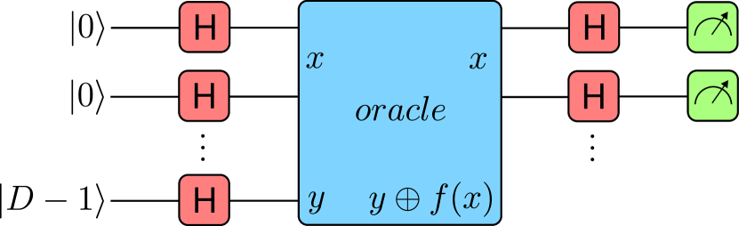
Figure 1: Quantum circuit diagram representing the generalized Deutsch-Josza algorithm for qudits. This configuration uses the state $|D-1\rangle$ for the last qudit and employs generalized Hadamard gates. The circuit is designed to test whether a given function, represented as a black box in the diagram, is constant or balanced across $d$-dimensional states (dits).

The extension of this algorithm to qudits is straightforward [32, 33], as illustrated in Figure 1. Instead of using the state $|1\rangle$ for the last qubit, we use the qudit state $|D-1\rangle$, where $D$ represents the dimension of the qudit. By measuring the register qudits, information is obtained in dits rather than bits, increasing the classical complexity to $D^{n-1}-1$ evaluations, while the quantum complexity remains constant.

To illustrate the practical implementation of the Deutsch-Josza algorithm for qudits, we provide a sample code using the library. The code below demonstrates how to set up the circuit for the algorithm, define an oracle function that can be either constant or balanced, and execute the necessary quantum operations to determine the nature of the function. By leveraging the flexibility of qudits, the circuit employs generalized Hadamard gates and measures the system in dits, reflecting the dimensionality $D$ of the qudits involved.

⬇

1import quforge as qf

2

3D = 3 #dimension of the qudit

4N = 4 #number of qudits

5

6#define oracle

7def oracle(model, mode=’constant’):

8 if mode == ’constant’:

9 model.X(index=[N-1])

10 else:

11 model.CNOT(index=[2,3])

12 return model

13

14#define circuit

15circuit = qf.Circuit(dim=D, wires=N)

16circuit.H(index=range(N))

17

18#apply oracle

19oracle(circuit, mode=’balanced’)

20

21# Hadamard on the first N-1 qudits

22circuit.H(index=range(N-1))

23

24#initial state

25state = ’’

26for i in range(N-1):

27 state += ’0-’

28state += ’%i’ % (D-1)

29state = qf.State(state, D=D)

30

31#Apply initial state in the circuit

32output = circuit(state)

33

34#Measure the first N-1 qudits

35_, p = qf.measure(output, index=range(N-1), D=D)

36

37if p[0] == 1:

38 print(’The function is constant’)

39else:

40 print(’The function is balanced’)

IV.2 Grover’s algorithm

Grover’s algorithm [34] is an important algorithm in the field of quantum computing, providing an optimized search mechanism for unstructured data. Classical search algorithms which operate with a complexity of $O(N)$, where $N$ represents the total number of items. Grover’s algorithm achieves a quadratic speed-up, demonstrating a complexity of $O(\sqrt{N})$. This improvement means that the algorithm can locate items within a database faster, on average.

Fundamentally, Grover’s algorithm is based on an oracle mechanism. It operates in two main phases: the oracle and diffusion stages. In the oracle phase, the desired item is marked by flipping its phase. Subsequently, the diffusion process amplifies the amplitude of this marked state, thereby increasing the probability that the correct item will be selected upon measurement. This sequence is iteratively repeated until the amplitude of the marked state is maximized. It is crucial to note that excessively repeating these iterations can inadvertently decrease the amplitude of the marked state due to the averaging effect introduced by the diffusion operator. Therefore, determining the optimal number of iterations is essential to maximize the effectiveness of the search.

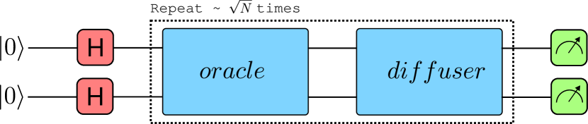
Figure 2: Quantum circuit diagram representing the generalized Grover’s algorithm. The circuit has an iterative part that is repeated at the order of $\sqrt{N}$ times. The oracle is responsible for flipping the phase of the marked state, while the diffusion step amplifies its amplitude.

When extending Grover’s algorithm to qudits [35, 36], the core principles largely remain unchanged, as shown in Figure 2. However, the use of qudits allows for a larger database capacity, albeit at the cost of an increased number of necessary iterations. A critical step involves achieving an equal superposition of all states before applying the algorithm itself, which can be accomplished by applying a generalized Hadamard gate to the $|0\rangle$ state.

To demonstrate the implementation of Grover’s algorithm for qudits using the QuForge library, the following code outlines the construction of a quantum circuit that searches for a marked state within an unstructured database. The code initializes the circuit by creating an equal superposition of all possible states using generalized Hadamard gates. It then iteratively applies the oracle, which marks the target state by flipping its phase, followed by the Grover diffusion step, which amplifies the probability amplitude of the marked state. By carefully choosing the number of iterations, the algorithm efficiently enhances the likelihood of identifying the marked state upon measurement.

⬇

1import quforge as qf

2

3D = 3 #dimension of the qudit

4N = 2 #number of qudits

5

6#define the oracle

7def oracle(circuit, register, marked_state):

8 basis = qf.zeros((9,1))

9 basis[8][0] = 1.0

10 target_state = basis @ basis.T

11

12 U = qf.kron(qf.eye(D), qf.eye(D)) - 2*target_state

13 circuit.Custom(M=U)

14

15#define the Grover diffusion step

16def grover_diffusion(circuit, register):

17 basis = qf.ones((D**N,1))/((D**N)**0.5)

18 U = 2*basis@basis.T - qf.eye(9)

19 circuit.Custom(M=U)

20

21#define circuit

22circuit = qf.Circuit(dim=D, wires=N)

23register = [i for i in range(N)]

24

25#apply Haddamard on each qudit

26circuit.H(index=register)

27

28#apply Grover’s algorithm

29num_iterations = int(round((2 ** 3) ** 0.5))

30for i in range(1):

31 # Apply the oracle

32 oracle(circuit, register, ’22’)

33

34 #Apply the diffusion

35 grover_diffusion(circuit, register)

36

37#initial state

38state = qf.State(’0-0’, D=D)

39

40#Apply the circuit on the initial state

41output = circuit(state)

42

43#Measure the first N-1 qudits

44histogram, p = qf.measure(output, index=register, D=D)

IV.3 Variational quantum algorithm

Variational Quantum Algorithms (VQAs) [37] are among the principal quantum algorithms used in machine learning. These algorithms employ parameterized circuits, which are optimized to minimize a loss function, thereby achieving a specific objective. The circuits consist of parameterized gates, typically rotation gates with adjustable angles, that are iteratively modified to produce the desired outcomes. Generally, VQAs are optimized using gradient-based methods, where inference is performed by a quantum computer (or simulator), and the optimization is carried out classically.

Extending VQAs to qudits offers multiple advantages. First, they provide a more nuanced representation of data as they are not constrained by binary representations, allowing for the encoding of more information with the same number of qudits. Additionally, qudits enable more expressive output representations, effectively compressing greater amounts of information into fewer qudits.

In this study, we demonstrate the application of qudit-based VQAs to two classification problems using the Iris and MNIST datasets, highlighting the advantages of qudits over qubits in specific scenarios.

The circuit configuration used in both classification tasks is depicted in Figure 3. The process initiates with all qudits in the zero state, represented as $|0\rangle^{\otimes N}$. Each qudit then undergoes transformation via a generalized Hadamard gate, preparing the state for feature encoding. This encoding involves setting the angles of $R_{z}$ rotation gates based on the input data features. Subsequently, the primary VQA circuit is employed, consisting of a series of rotation gates. This is followed by the application of generalized CNOT gates, which establish entanglement by coupling the first qudit with each subsequent qudit. The circuit concludes with a final series of rotation gates prior to measurement.

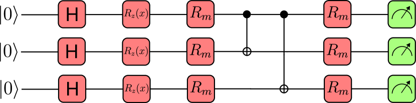
Figure 3: General quantum variational circuit chosen for this study. Hadamard gates are applied to the zero state before feature encoding of the data in order to prepare the input state for the algorithm. Then a number of rotation gates are applied followed by CNOT gates, and a second set of rotational gates are applied before measurement.

The selection of rotation gates, denoted as $R_{m}$, is contingent upon the dimensionality of the qudits and can be configured in various forms. We determine the index $m$ corresponding to each circuit configuration as outlined below:

• The first configuration, $R_{1}$, applies a sequence of rotation gates along the $z$, $y$, and $x$ axes to each qudit, restricted to the indexes $\{0,1\}$ for each gate, formally represented as:

  $$R_{1}|\psi\rangle=\prod_{i=x,y,z}R_{i}^{0,1}|\psi\rangle=R_{z}^{0,1}R_{y}^{0,1}R_{x}^{0,1}|\psi\rangle$$ (3)

• In the second configuration, $R_{2}$ rotation gates are applied across all axes with the index $j=0$ consistently maintained, while the index $k$ varies for the axes $x$ and $y$, and index $j$ varies for the axis $z$, as represented by:

  $$R_{2}|\psi\rangle=\prod_{i=x,y,z}\prod_{k}R_{i}^{0,k}|\psi\rangle$$ (4)

• The third configuration, $R_{3}$, extends the application of rotation gates along all axes, and combines all possible rotations by varying the indices $j$ and $k$, as described by:

  $$R_{3}|\psi\rangle=\prod_{i=x,y,z}\prod_{j,k}R_{i}^{j,k}|\psi\rangle$$ (5)

To further explore the implementation of qudit-based Variational Quantum Algorithms, we provide a code example using the library. The code defines a quantum variational circuit specifically designed for classification tasks, featuring an initial state preparation through generalized Hadamard gates, followed by feature encoding with $RZ$ rotation gates. The main variational circuit consists of multiple layers of rotation gates along different axes and generalized CNOT gates that establish entanglement among the qudits. This setup allows for flexible circuit configurations based on the chosen rotation gates, as described in the preceding sections. By adjusting the circuit parameters through a classical optimization loop, the model learns to minimize the loss function, thus achieving the desired classification outcomes. The following code outlines the circuit structure and demonstrates the process of initializing, encoding, and evolving the qudit states within the variational framework.

⬇

1import quforge as qf

2

3class QVA(qf.Module):

4 def __init__(self, dim, wires):

5 super(QVA, self).__init__()

6

7 self.init = qf.HGate(dim=dim, index=range(4))

8 self.encoder = qf.RZGate(dim=dim, index=range(4))

9

10 self.circuit = qf.Circuit(dim=dim, wires=wires)

11 self.circuit.RX(j=0, k=1, index=range(4)),

12 self.circuit.RX(j=1, k=2, index=range(4)),

13 self.circuit.RXGate(j=0, k=2, index=range(4)),

14 self.circuit.RYGate(j=0, k=1, index=range(4)),

15 self.circuit.RYGate(j=1, k=2, index=range(4)),

16 self.circuit.RYGate(j=0, k=2, index=range(4)),

17 self.circuit.RZGate(j=1, index=range(4)),

18 self.circuit.RZGate(j=2, index=range(4)),

19 self.circuit.CNOT(index=[0,1]),

20 self.circuit.CNOT(index=[1,2]),

21 self.circuit.CNOT(index=[2,3]),

22 self.circuit.RXGate(j=0, k=1, index=range(4)),

23 self.circuit.RXGate(j=1, k=2, index=range(4)),

24 self.circuit.RXGate(j=0, k=2, index=range(4)),

25 self.circuit.RYGate(j=0, k=1, index=range(4)),

26 self.circuit.RYGate(j=1, k=2, index=range(4)),

27 self.circuit.RYGate(j=0, k=2, index=range(4)),

28 self.circuit.RZGate(j=1, index=range(4)),

29 self.circuit.RZGate(j=2, index=range(4)),

30

31 def forward(self, x):

32 y = qf.State(’0-0-0-0’, D=self.D)

33 y = self.init(y)

34 y = self.encoder(y, param=x)

35 y = self.circuit(y)

36

37 return y

IV.3.1 Iris dataset

The Iris Flower dataset [38] comprises observations from 50 individual flowers distributed across three distinct species: Iris setosa, Iris virginica, and Iris versicolor. Each flower is described by four phenotypic attributes: Petal Length, Petal Width, Sepal Length, and Sepal Width.

In our approach, we utilize a quantum circuit with four qudits, where each qudit is responsible for phase encoding a specific attribute. Given the dataset’s classification into three species, we implement a qubit and a qutrit for categorical encoding. The qubit employs one-hot encoding to represent the three classes, defined by the target states as $|100\rangle$, $|010\rangle$ and $|001\rangle$, respectively, measured on the first three qubits. Concurrently, the qutrit is also used for one-hot encoding of the species classes, but with a focus on exploring the properties of high-dimensionality intrinsic to qudits. Here, we measure only the first qutrit, designating the target states as $|0\rangle$, $|1\rangle$, or $|2\rangle$.

The circuit is configured as described before, with the rotations gates chosen from the $R_{3}$ design. The dataset is partitioned into subsets, with 40 data points designated for training and the remaining $10$ are used for testing purposes. We conducted training across five different initializations to evaluate the mean classification accuracy.

Figure 4 illustrates the comparative results from each model configuration. The results indicate that by employing a dense encoding scheme for the qutrits yields superior accuracy compared to the alternate models. This enhancement suggests the potential benefits of leveraging the higher dimensionality of qudits in quantum variational algorithms.

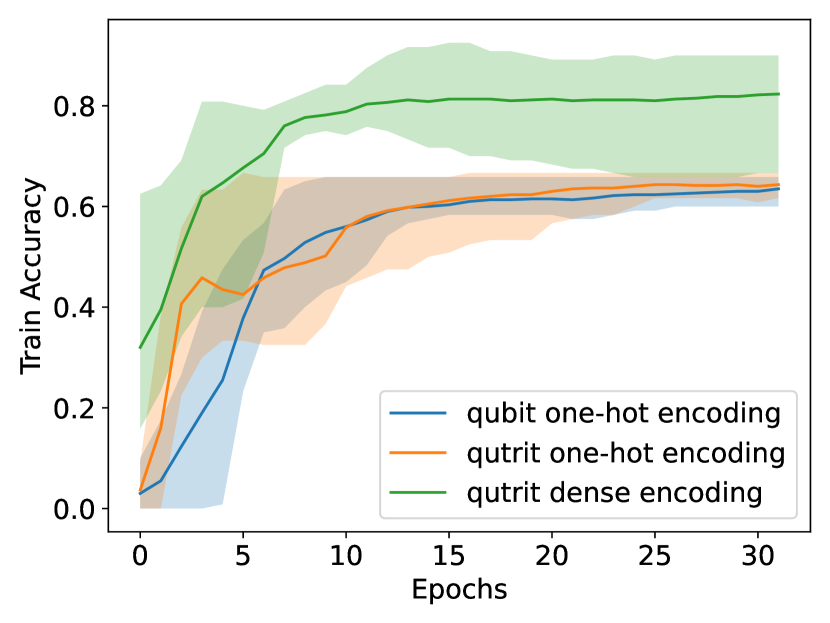
((a))

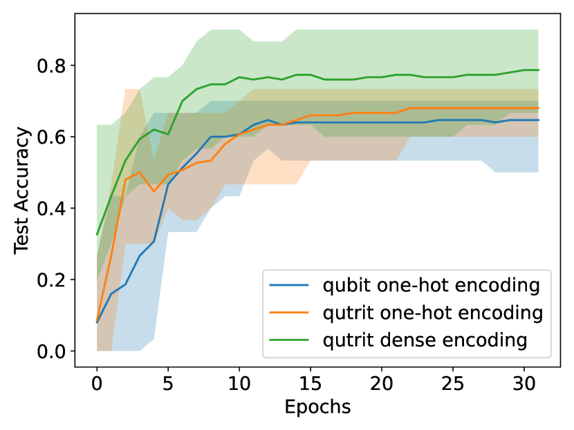
((b))

Figure 4: Mean accuracy of the Iris dataset for (a) training data and (b) test data for different dimension of qudits and types of encoding. The shaded regions indicate the lowest and highest accuracy obtained for each run.

IV.3.2 MNIST dataset

The MNIST dataset [39] comprises labeled images of handwritten digits ranging from 0 to 9, each represented in grayscale with a resolution of 28x28 pixels. Given the considerable dimensionality presented by the 784-pixel input space for quantum simulation, our methodology adopts a hybrid approach aimed at dimensionality reduction to minimize the requisite number of qudits for computational processing. This process involves the utilization of a classical linear layer model, comprising a single layer of neurons that condenses the 784-dimensional vector representation of each image into a compact form represented by the number of qudits available. Subsequently, phase encoding is applied to the output of each neuron, thereby preparing a quantum state for training a variational circuit.

Considering the dataset’s categorization into ten distinct classes, our model employs a ten-dimensional qudit to represent each class. This classification is quantified by measuring the state of the first qudit. For comparative analysis with traditional qubit-based circuits, we implement a circuit configured with ten qubits, utilizing a one-hot encoding scheme to represent each class.

In this study, a subset comprising 1000 randomly selected images serves as the training set, while an additional set of 500 randomly chosen images is designated for testing purposes. The efficacy of the proposed model is evaluated by calculating the mean accuracy across both datasets.

We applied the three designs of rotations gates in order to test different possible combinations. As depicted in Figure 5, our analysis reveals that utilizing at least two qudits not only achieves but exceeds the accuracies obtainable with a ten-qubit circuit. This observation suggests that qudits can offer superior representational efficiency with fewer quantum bits, highlighting their potential in quantum computations with qudits.

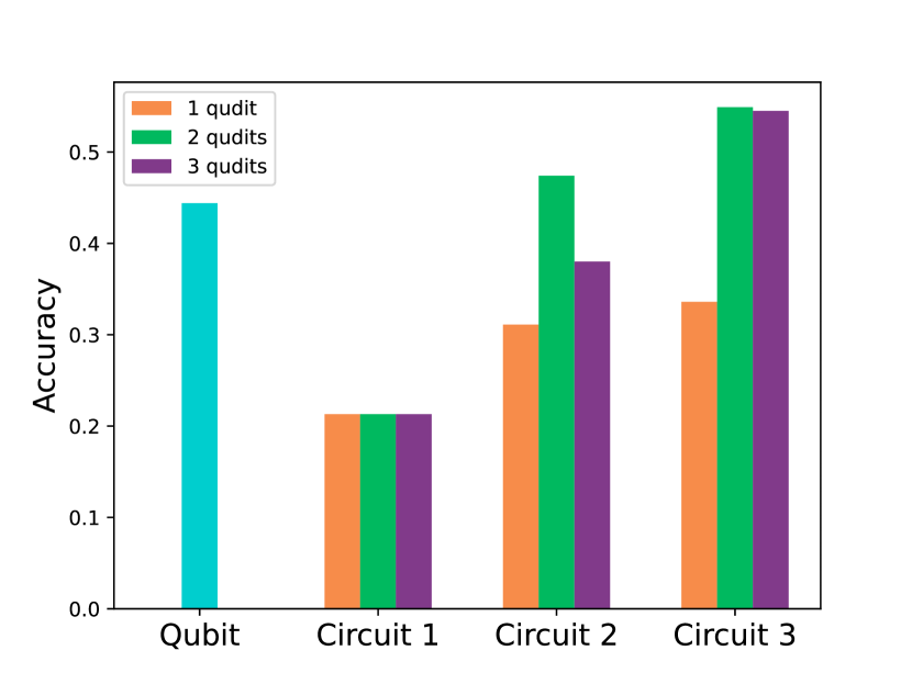
((a))

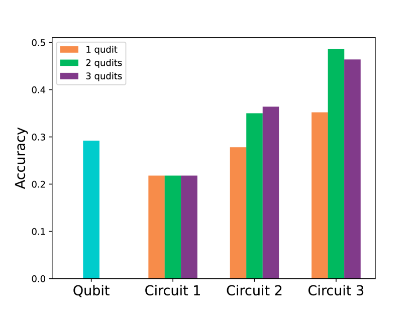
((b))

Figure 5: Mean accuracy for (a) training data and (b) test data across various circuits and qudit numbers. For shallow circuits (Circuit 1), qudits exhibit lower accuracy compared to qubits. However, with an increased number of rotation gates, qudit models (Circuits 2 and 3) surpass qubits in accuracy.

IV.4 Performance metrics

In this section, we present a performance evaluation of the qudit simulation library, benchmarking its execution on both CPU and GPU architectures, with and without the use of sparse gate representations. The performance is assessed for different number of qudits and qudit dimensions, providing a view of the scalability of the library. Two distinct time metrics are measured: the initialization time, representing the time required to construct the quantum circuit after its specification, and the execution time, indicating the duration needed to apply the circuit to a given input state.

To ensure robustness in the performance analysis, we conduct 10 independent trials for each configuration and compute the mean and standard deviation of the measured times. This approach enables us to quantify the sensitivity of the performance of the library to variations in execution conditions, analysing potential fluctuations in runtime, which may arise from factors such as hardware load or architectural differences.

We focus our evaluation on quantum variational circuits, as depicted in Figure 3, since they are very general for quantum machine learning. It is important to note, however, that the specific choice of circuit architecture and the types of quantum gates employed may influence both initialization and execution times. Therefore, while quantum variational circuits provide a solid benchmark for performance assessment, other circuit types may exhibit different timing characteristics depending on their structural complexity and gate set.

Figure 6 shows the initialization time of the qudit simulation library for up to four qudits across different qudit dimensions. The observed behavior demonstrates that initialization time is sensitive to both the number of qudits and the dimensionality of the qudit space. For a single qudit, the performance difference between the four configurations—CPU and GPU, with sparse and dense gate representations—is minimal. Sparse matrix representations show a slight advantage in initialization time over dense matrices, although this difference remains marginal.

However, as the number of qudits increases, the performance divergence becomes more pronounced. When simulating multiple qudits, sparse matrix representations consistently outperform dense representations, particularly on the CPU. Dense matrices on the CPU maintain an edge in performance only at very low qudit dimensions. For configurations with three and four qudits, the sparse matrix representation exhibits a significant reduction in initialization time compared to its dense counterpart, demonstrating clear scalability advantages in larger systems.

Notably, for systems with four qudits at high dimensions, the results suggest that sparse matrix operations on the GPU could potentially offer faster initialization times. However, in our experiments, this advantage was not fully realized due to memory limitations inherent to high-dimensional simulations on GPU hardware. It is important to highlight that sparse representations allow for simulations at higher qudit dimensions, thanks to their reduced memory relative to dense representations. This reduced memory consumption is particularly beneficial when scaling up the dimensionality of qudits, as it mitigates the memory overhead typically associated with dense quantum gate representations.

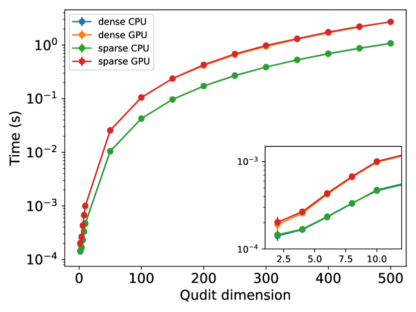
((a))

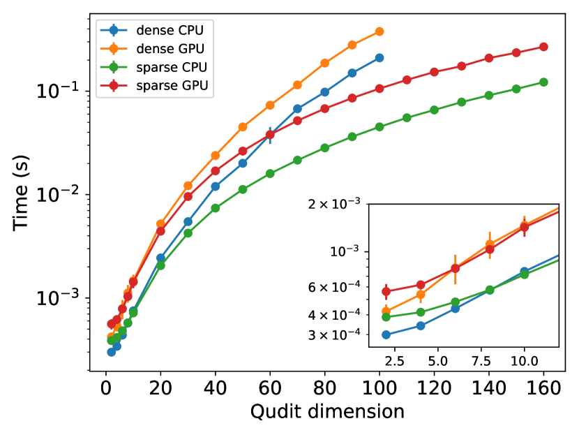
((b))

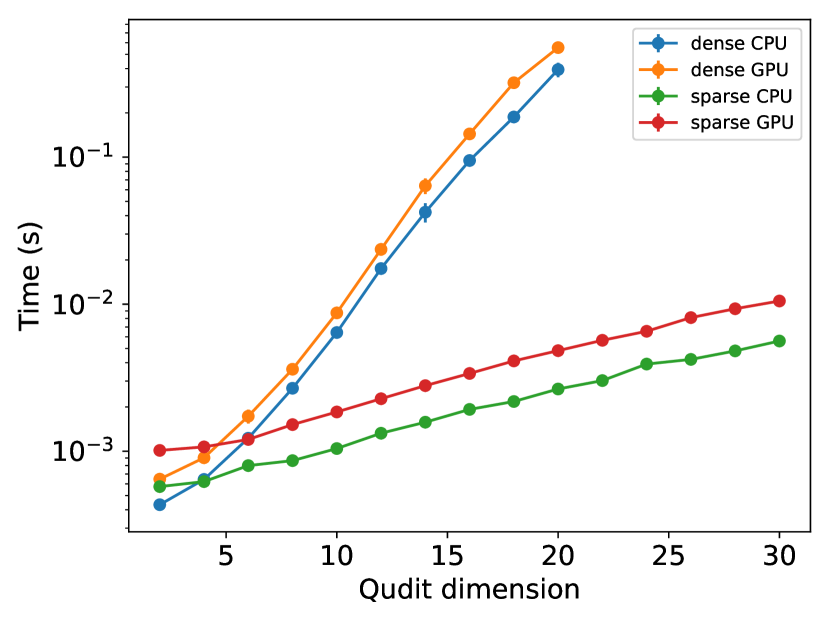
((c))

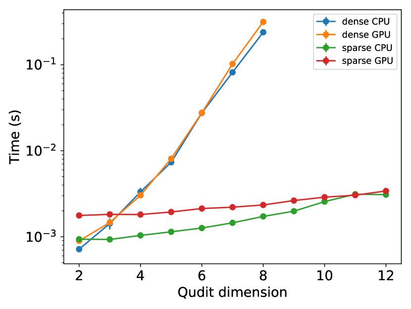
((d))

Figure 6: Initialization time as a function of the number of qudits and qudit dimensions: (a) 1 qudit, (b) 2 qudits, (c) 3 qudits and (d) 4 qudits. The comparison between CPU and GPU performance for both sparse and dense matrix representations shows that sparse matrices consistently result in faster initialization times as the number of qudits increases, particularly on the CPU. Although GPU performance at higher dimensions is constrained by memory limitations, sparse representations enable more efficient scaling to larger qudit systems.

Figure 7 presents the execution time of quantum circuits for varying numbers of qudits and qudit dimensions. For a single qudit at low dimensions, the CPU with dense matrix representations emerges as the fastest configuration. However, at very high dimensions, the sparse CPU representation becomes more advantageous, whereas the sparse GPU configuration is the slowest. This slowdown in the GPU sparse case for a single qudit is likely due to the relatively low sparsity of the matrices, which diminishes the benefits of sparse matrix operations in such configurations.

As the number of qudits increases, a clear trend emerges: sparse matrix representations on the GPU become the fastest at higher dimensions. For low dimensions, the CPU dense configuration remains the fastest, particularly at the lower end of the dimensional scale. However, as the dimensionality increases, both the GPU and sparse representations outperform dense CPU configurations, highlighting the efficiency gains in handling larger, more complex qudit systems with sparse matrices and GPU devices. As observed in the initialization time analysis, sparse matrix representations also enable the simulation of qudits at higher dimensions due to their significantly reduced memory requirements compared to dense matrices. This efficiency allows for the simulation of more complex systems, providing an advantage for high-dimensional quantum simulations.

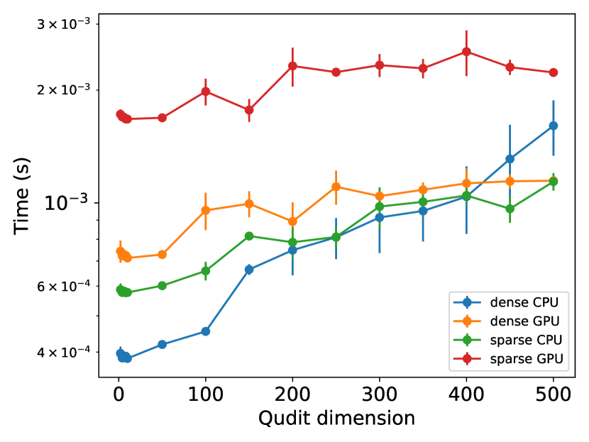
((a))

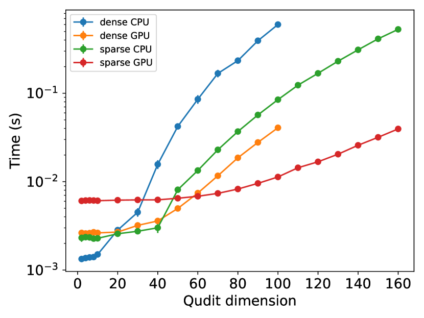
((b))

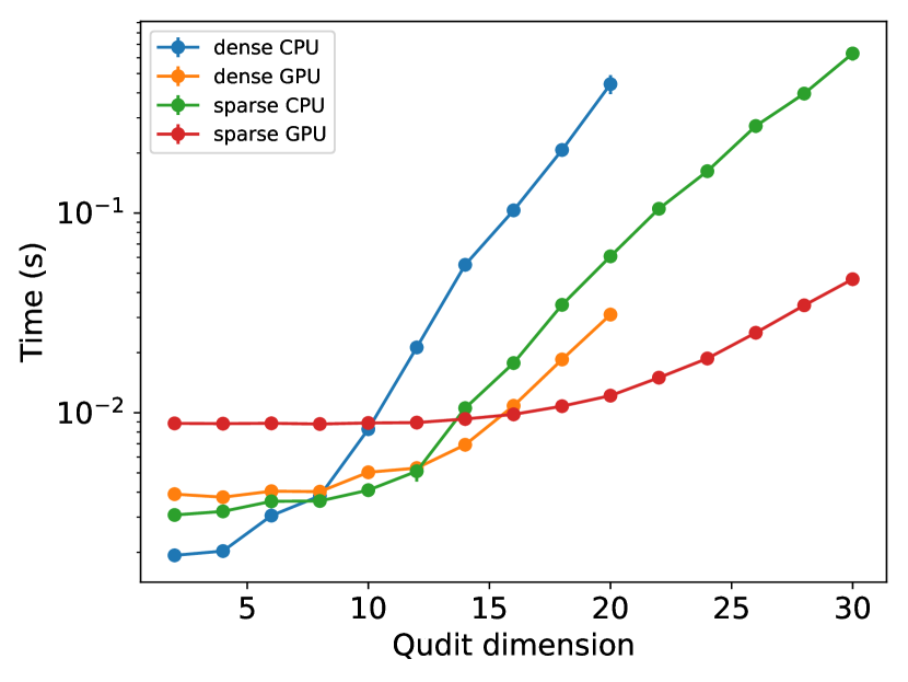
((c))

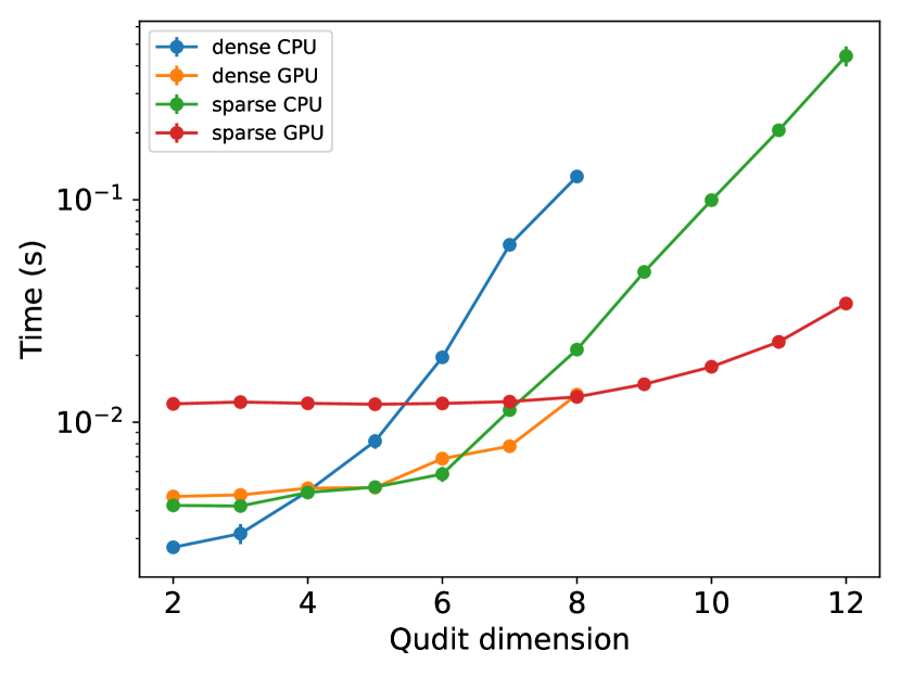
((d))

Figure 7: Execution time as a function of the number of qudits and qudit dimensions—(a) 1 qudit, (b) 2 qudits, (c) 3 qudits, and (d) 4 qudits—comparing CPU and GPU performance with sparse and dense matrix representations. For low dimensions, CPU dense matrices are the fastest, but as dimensionality and qudit count increase, GPU sparse representations show a performance advantage.

V Conclusion

In this article, we presented QuForge, a Python library for qudit simulation. QuForge was developed to facilitate the implementation of quantum algorithms by providing readily available quantum gates for qudits of any dimension. Built on top of PyTorch’s framework, QuForge allows seamless integration with various hardware platforms and leverages their computational power to speed up simulations. The library’s ability to construct differentiable graphs from quantum circuits is particularly advantageous for training quantum machine learning algorithms. This integration also simplifies the construction and training of hybrid classical-quantum algorithms, reducing the coding overhead typically associated with such tasks. Additionally, we explored the use of sparse representations for quantum gates, which significantly decreases the memory consumption of the library and accelerates its operations. This optimization is important for handling larger and more complex quantum systems efficiently.

However, the current limitations of the library include its restriction to simulating quantum circuits on classical computers. This limitation arises from the primary focus on qubits in existing quantum hardware, though there have been recent advancements in qudit implementations, especially in photonic and ion-trap quantum computers. Another limitation is that the library does not yet support the decomposition of qudit operations into qubit operations, which remains an open area of research. With the development of decomposition algorithms, it may be possible to integrate this functionality in the future.

Our goal with QuForge is to provide the scientific community with a high-level tool for conducting research on qudits. By abstracting the complexities of hardware operations, QuForge enables researchers to focus on developing and testing quantum algorithms, thereby helping in advancing the field of qudit quantum computing.

Data availability

The code for the QuForge library, along with the examples shown in this article, can be found at https://github.com/tiago939/QuForge.

Appendix A Matrix form of the quantum gates

This appendix provides a comprehensive and detailed construction of the quantum gates. Each gate is described, with explicit definitions of their respective operations. Furthermore, when feasible, the derivation of the sparse matrix representation for each gate is presented. Table 2 summarizes the main gates available.

Single qudit gates	Two-qudit gates
NOT, Eq. (A.1)	CNOT, Eq. (A.6)
Phase-shift, Eq. (A.2)	SWAP, Eq. ( A.7)
Fourier, Eq. (A.3)	Controlled Rotation, Eq. (A.8)

Table 2: Overview of the primary single-qudit and two-qudit gates available in the QuForge library.

A.1 Generalized NOT gate

The $X$ gate, also known as the $NOT$ gate, is fundamental for qubits. It performs a bit-flip operation, transforming the state of a qubit from $|0\rangle$ to $|1\rangle$ and vice versa. When dealing with qudits, the analogous operation is more intricate. The $X$ gate in this context performs a modulus sum on the qudit’s value. Typically, this summand, denoted as $s$, is set to 1, although other values can be used depending on the desired operation. Consequently, this gate induces a cyclic permutation of the qudit states. For example, in a three-level system, the application of the $X$ gate results in the following transitions: $|0\rangle\rightarrow|1\rangle\rightarrow|2\rangle\rightarrow|0\rangle$. This gate has the following representation:

$$X^{D}_{s}|x\rangle=|x+s\bmod D\rangle.$$ (6)

A.2 Generalized phase-shift gate

Phase-shift gates are essential components in quantum computing, particularly for manipulating the phase of qudits in $D$-level quantum systems. These gates adjust the amplitude of the qudit states by applying a phase factor. Let $\omega=e^{2\pi i/D}$, where $D$ denotes the dimension of the qudit. The phase-shift gate operates as follows: it leaves the state $|0\rangle$ unchanged, i.e., $|0\rangle\rightarrow|0\rangle$, while transforming the state $|1\rangle$ to $\omega|1\rangle$, the state $|2\rangle$ to $\omega^{2}|2\rangle$, and so forth. This progression continues cyclically through all $D$ states. The general transformation for a state $|k\rangle$ can be expressed as $|k\rangle\rightarrow\omega^{k}|k\rangle$.

The corresponding unitary matrix representation of this phase-shift gate, denoted as $P$, is a diagonal matrix with the elements $\{1,\omega,\omega^{2},...,\omega^{D-1}\}$ along its diagonal. Formally, the matrix is given by:

$$P=\begin{bmatrix}1&0&0&...&0\\ 0&\omega&0&...&0\\ 0&0&\omega^{2}&...&0\\ \vdots&\vdots&\vdots&\vdots&\vdots\\ 0&0&0&...&w^{D-1}\end{bmatrix}.$$ (7)

A.3 Fourier gate

The Fourier gate, also referred to as the generalized Hadamard gate, plays an important role in quantum computing by enabling the creation of superposition states. The nature of the superposition generated by this gate depends intricately on the initial state of the qudit to which it is applied. When applied to the state $|0\rangle$, the Fourier gate produces an equal superposition of all $D-1$ possible states, each with identical amplitude. For other initial states, the resulting amplitudes vary according to the specific starting state of the qudit, thereby introducing a rich structure of quantum superpositions.

The matrix representation of the Fourier gate, denoted as $H$, is derived from the principles of the discrete Fourier transform. This matrix can be expressed as:

$$H=\frac{1}{\sqrt{D}}\begin{bmatrix}1&1&1&...&1\\ 1&\omega&\omega^{2}&...&\omega^{D-1}\\ 1&\omega^{2}&\omega^{4}&...&\omega^{2(D-1)}\\ \vdots&\vdots&\vdots&\vdots&\vdots\\ 1&\omega^{D-1}&\omega^{2(D-1)}&...&\omega^{(D-1)^{2}}\end{bmatrix}.$$ (8)

The factor $\frac{1}{\sqrt{D}}$ ensures the normalization of the transformation, maintaining the unitary property of the gate.

A.4 Generalized Gell-Mann matrices

The generalized Gell-Mann matrices, also known as generalized Pauli matrices, are important in the context of rotation gates in quantum computing. These matrices extend the concept of the Pauli matrices to higher-dimensional systems and play an important role in defining rotations and other transformations in $D$-level quantum systems. They come in three distinct forms: symmetric, anti-symmetric, and diagonal.

Let $j$ and $k$ be indices ranging from 0 to $D-1$. The generalized Gell-Mann matrices are defined as follows:

1. Symmetric form:

   $$S_{x}^{jk} =|j\rangle\langle k|+|k\rangle\langle j|.$$ (9)

   This matrix, with indexes $0\leq j<D$ and $0\leq k<D$, represents a symmetric combination of the basis states $|j\rangle$ and $|k\rangle$, facilitating rotations that symmetrically affect these states.

2. Anti-symmetric form:

   $$S_{y}^{jk} =-i|j\rangle\langle k|+i|k\rangle\langle j|.$$ (10)

   Here, the anti-symmetric form introduces an imaginary component, with indexes $0\leq j<D$ and $0\leq k<D$, useful for generating rotations that are skew-symmetric, affecting the states $|j\rangle$ and $|k\rangle$ with opposite phases.

3. Diagonal form:

   $$S_{z}^{j} =\sqrt{\frac{2}{j(j+1)}}\sum_{k=1}^{j}(-j)^{\delta(k,j)}|k\rangle\langle k|$$ (11)

   The diagonal form of the matrix is defined for each $0\leq j<D$ and involves a summation over the basis states up to $j$. The Kronecker delta $\delta(k,j)$ ensures that the contribution is weighted appropriately, introducing a factor that depends on the index $j$.

A.5 Generalized rotation gate

Rotation gates are among the most crucial elements in quantum machine learning, owing to their ability to introduce tunable parameters that can be optimized to achieve specific outcomes in quantum circuits. These gates are characterized by an angle parameter $\theta$, which can be adjusted during the training of a quantum algorithm to fine-tune the performance of the quantum model. The implementation of rotation gates relies fundamentally on the generalized Gell-Mann matrices. These matrices serve as the generators for the rotations, controlling the axis and nature of the rotation within the $D$-dimensional quantum state space. The general form of a rotation gate is given by:

$$R_{\alpha}=e^{-i\theta S_{\alpha}/2},$$ (12)

where $S_{\alpha}$ represents the generalized Gell-Mann matrix, and $\alpha$ denotes the type of the matrix (symmetric, anti-symmetric, or diagonal).

In practical applications, the parameter $\theta$ is typically adjusted using optimization algorithms to minimize a cost function, thereby enabling the quantum circuit to learn and perform specific tasks effectively. This process is analogous to adjusting weights in classical machine learning models. The flexibility offered by rotation gates makes them fundamental in the construction of variational quantum circuits, which are central to many quantum machine learning frameworks.

For the sparse form of the rotation gate, we start from

$$R_{\alpha}^{j,k}(\theta)=e^{-i\theta S_{\alpha}^{j,k}/2},$$ (13)

with $\alpha=x,y,z$. To better understand the construction and action of these rotation gates, we can explore specific cases and then generalize the pattern.

Case $D=2$. For $D=2$, we have a single possibility for each direction:

$$S_{x}^{1,2} =|1\rangle\langle 2|+|2\rangle\langle 1|=\begin{bmatrix}0&1\\ 1&0\end{bmatrix},$$ (14)

$$S_{y}^{1,2} =-i|1\rangle\langle 2|+i|2\rangle\langle 1|=\begin{bmatrix}0&-i\\ i&0\end{bmatrix},$$ (15)

$$S_{z}^{1} =\sum_{k=1}^{2}\sqrt{1}(-1)^{\delta_{k,2}}|k\rangle\langle k|$$

$$=|1\rangle\langle 1|-|2\rangle\langle 2|=\begin{bmatrix}1&0\\ 0&-1\end{bmatrix}.$$ (16)

Here, the states $|1\rangle$ and $|2\rangle$ form the computational basis for the qubit system. The corresponding rotation matrices for $D=2$ are:

$$R_{x}^{1,2}(\theta)=e^{-i\theta S_{x}^{1,2}/2}=e^{(-i\theta/2)(|+\rangle\langle+|-|-\rangle\langle-|)}$$

$$=\begin{bmatrix}\cos(\theta/2)&-i\sin(\theta/2)\\ -i\sin(\theta/2)&\cos(\theta/2)\end{bmatrix},$$ (17)

$$R_{y}^{1,2}(\theta)=e^{-i\theta S_{y}^{1,2}/2}=e^{(-i\theta/2)(|\oplus\rangle\langle\oplus|-|\ominus\rangle\langle\ominus|)}$$

$$=\begin{bmatrix}\cos(\theta/2)&-\sin(\theta/2)\\ \sin(\theta/2)&\cos(\theta/2)\end{bmatrix},$$ (18)

$$R_{z}^{1}(\theta)=e^{-i\theta S_{z}^{1}/2}=e^{(-i\theta/2)(|1\rangle\langle 1|-|2\rangle\langle 2|)}$$

$$=\begin{bmatrix}e^{-i\theta/2}&0\\ 0&e^{i\theta/2}\end{bmatrix},$$ (19)

with $|\pm\rangle=(|1\rangle\pm|2\rangle)/\sqrt{2}$, $|\oplus\rangle=(|1\rangle+i|2\rangle)/\sqrt{2}$, and $|\ominus\rangle=(|1\rangle-i|2\rangle)/\sqrt{2}$.

Case for $D=3$. For $D=3$, we consider a few examples to identify the general pattern:

$$S_{x}^{1,2}=|1\rangle\langle 2|+|2\rangle\langle 1|=\begin{bmatrix}0&1&0\\ 1&0&0\\ 0&0&0\end{bmatrix}.$$ (20)

Thus

$$R_{x}^{1,2}(\theta) =e^{-i\theta S_{x}^{1,2}/2}=e^{(-i\theta/2)(|+\rangle\langle+|-|-\rangle\langle-|)}$$

$$=\begin{bmatrix}\cos(\theta/2)&-i\sin(\theta/2)&0\\ -i\sin(\theta/2)&\cos(\theta/2)&0\\ 0&0&1\end{bmatrix}.$$ (21)

Case for $D=4$. For $D=4$, let us consider

$$S_{x}^{1,2}=|1\rangle\langle 2|+|2\rangle\langle 1|=\begin{bmatrix}0&1&0&0\\ 1&0&0&0\\ 0&0&0&0\\ 0&0&0&0\end{bmatrix}.$$ (22)

Thus

$$R_{x}^{1,2}(\theta) =e^{-i\theta S_{x}^{1,2}/2}=e^{(-i\theta/2)(|+\rangle\langle+|-|-\rangle\langle-|)}$$

$$=\begin{bmatrix}\cos(\theta/2)&-i\sin(\theta/2)&0&0\\ -i\sin(\theta/2)&\cos(\theta/2)&0&0\\ 0&0&1&0\\ 0&0&0&1\end{bmatrix}.$$ (23)

In the general case, this pattern repeats for any dimension. Specifically, the two-dimensional rotation is applied in the subspace with indices $j,k$, while the identity operation is applied to the rest of the vector space. Then, the non-zero elements of $R_{x}^{j,k}$ are:

$$\langle j|R_{x}^{j,k}(\theta)|j\rangle=\langle k|R_{x}^{j,k}(\theta)|k\rangle=\cos(\theta/2),$$ (24)

$$\langle j|R_{x}^{j,k}(\theta)|k\rangle=\langle k|R_{x}^{j,k}(\theta)|j\rangle=-i\sin(\theta/2),$$ (25)

$$\langle l|R_{x}^{j,k}(\theta)|l\rangle=1,\quad l\neq j\ \text{and}\ l\neq k.$$ (26)

And the non-zero elements of $R_{y}^{j,k}$ are:

$$\langle j|R_{y}^{j,k}(\theta)|j\rangle=\langle k|R_{y}^{j,k}(\theta)|k\rangle=\cos(\theta/2),$$ (27)

$$\langle j|R_{y}^{j,k}(\theta)|k\rangle=-\langle k|R_{y}^{j,k}(\theta)|j\rangle=-\sin(\theta/2),$$ (28)

$$\langle l|R_{y}^{j,k}(\theta)|l\rangle=1,\quad l\neq j\ \text{and}\ l\neq k,$$ (29)

while the non-zero elements of $R_{z}^{j}$ are:

$$\langle k|R_{z}^{j}(\theta)|k\rangle=\exp\left(-i\frac{\theta}{2}\sqrt{\frac{2}{j(j+1)}}(-j)^{\delta_{k,j+1}}\right),$$ (30)

for $k=1,\cdots,j-1$ and

$$\langle k|R_{z}^{j}(\theta)|k\rangle=1$$ (31)

for $k=j,\cdots,d.$

A.6 Generalized CNOT gate

The generalized CNOT gate, also known as the CX gate, is a fundamental two-qudit gate in quantum computing, essential for creating entanglement between two qudits. This gate operates with two components: the control qudit and the target qudit. The role of the CNOT gate is to preserve the state of the control qudit while modifying the state of the target qudit based on the value of the control qudit by applying an X gate.

The functionality of the generalized CNOT gate can be described as follows: if the control qudit is in the state $|x\rangle$, the state of the target qudit is changed to $|x+y\bmod D\rangle$, effectively performing an addition modulo $D$, as defined with the $X$ gate. Mathematically, the action of the generalized CNOT gate is represented by:

$$CNOT_{x\rightarrow y}|x\rangle|y\rangle=\begin{cases}|x\rangle|x+a\mbox{ mod }D\rangle,\mbox{ if }x=d-1\\ |x\rangle|y\rangle,\mbox{ otherwise }\end{cases}\,.$$ (32)

A computational basis state of N qudits can be represented as:

$$|j_{0}\rangle\otimes|j_{1}\rangle\otimes\cdots\otimes|j_{N-2}\rangle\otimes|j_{N-1}\rangle$$ (33)

$$\equiv|j_{0}j_{1}\cdots j_{N-2}j_{N-1}\rangle\equiv|j\rangle,$$ (34)

where the local state index $j_{s}$ ranges from $0$ to $D-1$, and the qudit index $s$ ranges from $0$ to $N-1$. The correspondence to the global state index, known as the decimal representation, is calculated as follows:

$$j=\sum_{k=0}^{N-1}j_{k}d^{N-1-k}.$$ (35)

To determine the non-zero elements of the CNOT gate matrix for N qudits, we need to consider the control qudit (denoted by index $c$) and the target qudit (denoted by index $t$). Depending on the relative positions of $c$ and $t$ (i.e., whether $c<t$ or $c>t$, the non-zero elements of the CNOT gate matrix are obtained as follows: $\bullet$ For $c<t$:

$$\langle\cdots,k_{c-1},k_{c},k_{c+1},\cdots,k_{t-1},k_{t}\oplus k_{c},k_{t+1},\cdots|C_{x}|\cdots,k_{c-1},k_{c},k_{c+1},\cdots,k_{t-1},k_{t},k_{t+1},\cdots\rangle=1.$$ (36)

$\bullet$ For $c>t$:

$$\langle\cdots,k_{t-1},k_{t}\oplus k_{c},k_{t+1},\cdots,k_{c-1},k_{c},k_{c+1},\cdots|C_{x}|\cdots,k_{t-1},k_{t},k_{t+1},\cdots,k_{c-1},k_{c},k_{c+1},\cdots\rangle=1$$ (37)

In both cases, $\oplus$ denotes addition modulo $D$. To generate the non-zero elements of the CNOT gate matrix, we start by generating all possible sequences of local basis states for N qudits, each of dimension $D$. These sequences correspond to the computational basis states $|j_{0},j_{1},...,j_{N-2},j_{N-1}\rangle$. The decimal representation of these sequences gives us the matrix indices for the right-hand side of the matrix element.

Next, we apply the transformation $j_{t}\rightarrow j_{t}\oplus j_{c}$ to obtain the matrix index for the left-hand side corresponding to the target qudit. This process ensures that we correctly identify the positions of the non-zero elements in the CNOT gate matrix, reflecting the gate’s action of conditionally flipping the target qudit’s state based on the control qudit’s state.

A.7 Generalized SWAP Gate

The SWAP gate is a two-qudit gate, designed to exchange the states of two qudits. This gate performs a simple operation, swapping the state of the first qudit with that of the second qudit. The action of the SWAP gate can be mathematically described as follows:

$$SWAP|x\rangle\otimes|y\rangle=|y\rangle\otimes|x\rangle$$ (38)

Here, $|x\rangle$ and $|y\rangle$ represent the states of the two qudits. When the SWAP gate is applied to the tensor product of these states, it interchanges them, resulting in the state $|y\rangle\otimes|x\rangle$.

For two qudits, the non-zero elements of the SWAP gate matrix are determined by examining how the gate acts on the basis states. The matrix element $\langle l,m|SWAP|p,q\rangle$ represents the overlap between the basis states $|l,m\rangle$ and $|p,q\rangle$. When the SWAP gate is applied, it exchanges the states of the two qudits, meaning that $SWAP|p,q\rangle$ results in $|q,p\rangle$. Therefore, the non-zero elements are found where the original states $|p,q\rangle$ and the swapped states $|l,m\rangle$ match, which occurs if and only if $l=q$ and $m=p$. This condition is mathematically expressed using the Kronecker delta function: $\delta_{l,p}\delta_{m,q}$.

For an $N$-qudit system, applying the SWAP gate to qudits $c$ and $t$ involves a similar procedure but within a larger state space. The matrix element $\langle j|SWAP_{c\leftrightarrow t}|k\rangle$ reflects the action of the SWAP gate on multi-qudit states. Here, the SWAP gate exchanges the states of the $c$-th and $t$-th qudits while leaving the other qudits’ states unchanged.

To find the non-zero elements, consider the basis state $|\cdots k_{c-1}k_{c}k_{c+1}\cdots k_{t-1}k_{t}k_{t+1}\cdots\rangle$. After applying the SWAP gate, this state transforms to $|\cdots k_{c-1}k_{t}k_{c+1}\cdots k_{t-1}k_{c}k_{t+1}\cdots\rangle$. Therefore, the matrix element $\langle j|SWAP_{c\leftrightarrow t}|k\rangle$ is non-zero when the sequence of indices $j$ matches this swapped configuration.

Explicitly, this means that the conditions for non-zero elements are:

$$\langle\cdots j_{c-1}j_{c}j_{c+1}\cdots j_{t-1}j_{t}j_{t+1}\cdots|\cdots k_{c-1}k_{t}k_{c+1}\cdots k_{t-1}k_{c}k_{t+1}\cdots\rangle$$ (39)

$$=\cdots\delta_{j_{c-1},k_{c-1}}\delta_{j_{c},k_{t}}\delta_{j_{c+1},k_{c+1}}\cdots\delta_{j_{t-1},k_{t-1}}\delta_{j_{t},k_{c}}\delta_{j_{t+1},k_{t+1}}\cdots$$ (40)

Thus, to determine the non-zero elements of the SWAP matrix, we systematically identify pairs of states $j$ and $k$ that satisfy these delta conditions, effectively swapping the $c$-th and $t$-th components while leaving the others unchanged.

A.8 Controlled Rotation Gate

The controlled rotation gate performs an operation similar to the generalized CNOT gate. It preserves the state of the control qudit while applying a rotation gate to the target qudit. In this context, the controlled rotation gate can be viewed as a more general form of the CNOT gate. Specifically, when the controlled rotation gate uses the symmetric form of the generalized Gell-Mann matrices and an angle $\theta=\pi$, it replicates the behavior of the CNOT gate.

To formalize this gate, it is essential to note that previous definitions, such as the one in reference [40], describe a non-differentiable controlled gate that does not align with the controlled rotation gate for qubits. Hence, we propose a new differentiable version of the controlled rotation gate that maintains equivalence for qubits while extending its applicability to qudits.

The differentiable controlled rotation gate is defined as:

$$C^{c\rightarrow t}_{R^{jk}_{\alpha}(\theta)}=\sum_{m=0}^{D-1}|m\rangle\langle m|\otimes R^{jk}_{\alpha}(m\theta),$$ (41)

with $R^{jk}_{\alpha}(\theta)=e^{-i\theta S^{jk}_{\alpha}/2}.$ In this expression, the gate operates on two qudits: the control qudit ($c$) and the target qudit ($t$). The operator $|m\rangle\langle m|$ acts as a projector on the control qudit, ensuring that the rotation is conditioned on the state of the control qudit. The term $e^{-im\theta S_{\alpha}/2}$ represents the rotation applied to the target qudit, with $S_{\alpha}$ being the generalized Gell-Mann matrix. This construction ensures that the controlled rotation gate is smooth and differentiable, which is important for optimization tasks in quantum machine learning. By enabling precise control over rotations, this gate facilitates the implementation of complex quantum algorithms that leverage the rich structure of qudit systems.

Regarding the sparse implementation of the controlled rotation gate, let us define e.g. $\mathbf{j}=\cdots,k_{c-1},k_{c},k_{c+1},\cdots,k_{t-1},j,k_{t+1},\cdots$ if $t>c$ and $\mathbf{j}=\cdots,k_{t-1},j,k_{t+1},\cdots,k_{c-1},k_{c},k_{c+1},\cdots$ if $t<c$, where $k_{s}=0,\cdots,d-1$ and $s=1,\cdots,N$ with $N$ being the number of qudits and $d$ is the dimension of each qudit. For the $x$-type rotations, the non-null elements are

$$\langle\mathbf{j}|C^{c\rightarrow t}_{R^{jk}_{x}(\theta)}|\mathbf{j}\rangle=\langle\mathbf{k}|C^{c\rightarrow t}_{R^{jk}_{x}(\theta)}|\mathbf{k}\rangle=\cos(k_{c}\theta/2),$$ (42)

$$\langle\mathbf{j}|C^{c\rightarrow t}_{R^{jk}_{x}(\theta)}|\mathbf{k}\rangle=\langle\mathbf{k}|C^{c\rightarrow t}_{R^{jk}_{x}(\theta)}|\mathbf{j}\rangle=-i\sin(k_{c}\theta/2),$$ (43)

$$\langle\mathbf{l}|C^{c\rightarrow t}_{R^{jk}_{x}(\theta)}|\mathbf{l}\rangle=1;\ l=0,\cdots,d-1;\ l\neq j,l\neq k.$$ (44)

In the case of the $y$-type rotations, the non-null elements are given by

$$\langle\mathbf{j}|C^{c\rightarrow t}_{R^{jk}_{y}(\theta)}|\mathbf{j}\rangle=\langle\mathbf{k}|C^{c\rightarrow t}_{R^{jk}_{x}(\theta)}|\mathbf{k}\rangle=\cos(k_{c}\theta/2),$$ (45)

$$\langle\mathbf{j}|C^{c\rightarrow t}_{R^{jk}_{y}(\theta)}|\mathbf{k}\rangle=\langle\mathbf{k}|C^{c\rightarrow t}_{R^{jk}_{x}(\theta)}|\mathbf{j}\rangle=-\sin(k_{c}\theta/2),$$ (46)

$$\langle\mathbf{l}|C^{c\rightarrow t}_{R^{jk}_{y}(\theta)}|\mathbf{l}\rangle=1;\ l=0,\cdots,d-1;\ l\neq j,l\neq k.$$ (47)

For the $z$-type rotations, the non-null elements are

$$\langle\mathbf{k}|C_{R_{z}^{j}(\theta)}^{c\rightarrow t}|\mathbf{k}\rangle=\exp\Big{(}-i\frac{k_{c}\theta}{2}\sqrt{\frac{2}{j(j+1)}}(-j)^{\delta_{k,j+1}}\Big{)}$$ (48)

for $k=1,\cdots,j+1$ and

$$\langle\mathbf{k}|C_{R_{z}^{j}(\theta)}^{c\rightarrow t}|\mathbf{k}\rangle=1$$ (49)

for $k=j+2,\cdots,d.$

References

- Paszke et al. [2019] A. Paszke, S. Gross, F. Massa, A. Lerer, J. Bradbury, G. Chanan, T. Killeen, Z. Lin, N. Gimelshein, L. Antiga, A. Desmaison, A. Köpf, E. Yang, Z. DeVito, M. Raison, A. Tejani, S. Chilamkurthy, B. Steiner, L. Fang, J. Bai, and S. Chintala, Pytorch: An imperative style, high-performance deep learning library (2019), arXiv:1912.01703 .
- Bradbury et al. [2018] J. Bradbury, R. Frostig, P. Hawkins, M. J. Johnson, C. Leary, D. Maclaurin, G. Necula, A. Paszke, J. VanderPlas, S. Wanderman-Milne, and Q. Zhang, JAX: composable transformations of Python+NumPy programs (2018).
- Blondel and Roulet [2024] M. Blondel and V. Roulet, The elements of differentiable programming (2024), arXiv:2403.14606 .
- Goodfellow et al. [2016] I. Goodfellow, Y. Bengio, and A. Courville, Deep Learning (The MIT Press, 2016).
- Jouppi et al. [2017] N. P. Jouppi, C. Young, N. Patil, D. Patterson, G. Agrawal, R. Bajwa, S. Bates, S. Bhatia, N. Boden, A. Borchers, R. Boyle, P. luc Cantin, C. Chao, C. Clark, J. Coriell, M. Daley, M. Dau, J. Dean, B. Gelb, T. V. Ghaemmaghami, R. Gottipati, W. Gulland, R. Hagmann, C. R. Ho, D. Hogberg, J. Hu, R. Hundt, D. Hurt, J. Ibarz, A. Jaffey, A. Jaworski, A. Kaplan, H. Khaitan, A. Koch, N. Kumar, S. Lacy, J. Laudon, J. Law, D. Le, C. Leary, Z. Liu, K. Lucke, A. Lundin, G. MacKean, A. Maggiore, M. Mahony, K. Miller, R. Nagarajan, R. Narayanaswami, R. Ni, K. Nix, T. Norrie, M. Omernick, N. Penukonda, A. Phelps, J. Ross, M. Ross, A. Salek, E. Samadiani, C. Severn, G. Sizikov, M. Snelham, J. Souter, D. Steinberg, A. Swing, M. Tan, G. Thorson, B. Tian, H. Toma, E. Tuttle, V. Vasudevan, R. Walter, W. Wang, E. Wilcox, and D. H. Yoon, In-datacenter performance analysis of a tensor processing unit (2017), arXiv:arXiv:1704.04760 .
- Chae et al. [2024] E. Chae, J. Choi, and J. Kim, An elementary review on basic principles and developments of qubits for quantum computing, Nano Convergence 11, 10.1186/s40580-024-00418-5 (2024).
- Brylinski and Brylinski [2001] J.-L. Brylinski and R. Brylinski, Universal quantum gates (2001), arXiv:quant-ph/0108062 .
- Wach et al. [2023] N. L. Wach, M. S. Rudolph, F. Jendrzejewski, and S. Schmitt, Data re-uploading with a single qudit, Quantum Machine Intelligence 5, 10.1007/s42484-023-00125-0 (2023).
- Goyal et al. [2014] S. K. Goyal, P. E. Boukama-Dzoussi, S. Ghosh, F. S. Roux, and T. Konrad, Qudit-Teleportation for photons with linear optics, Scientific Reports 4, 4543 (2014).
- Ogunkoya et al. [2024] O. Ogunkoya, J. Kim, B. Peng, A. B. i. e. i. f. m. c. Özgüler, and Y. Alexeev, Qutrit circuits and algebraic relations: A pathway to efficient spin-1 hamiltonian simulation, Phys. Rev. A 109, 012426 (2024).
- Tacchino et al. [2021] F. Tacchino, A. Chiesa, R. Sessoli, I. Tavernelli, and S. Carretta, A proposal for using molecular spin qudits as quantum simulators of light-matter interactions, Journal of Materials Chemistry C 9, 10266 (2021).
- Bourennane et al. [2001] M. Bourennane, A. Karlsson, and G. Björk, Quantum key distribution using multilevel encoding, Phys. Rev. A 64, 012306 (2001).
- Litteken et al. [2022] A. Litteken, J. M. Baker, and F. T. Chong, Communication trade offs in intermediate qudit circuits, in 2022 IEEE 52nd International Symposium on Multiple-Valued Logic (ISMVL) (2022) pp. 43–49.
- Chizzini et al. [2022] M. Chizzini, L. Crippa, L. Zaccardi, E. Macaluso, S. Carretta, A. Chiesa, and P. Santini, Quantum error correction with molecular spin qudits, Physical Chemistry Chemical Physics 24, 20030 (2022).
- Scott and Tůma [2023] J. Scott and M. Tůma, An introduction to sparse matrices, in Algorithms for Sparse Linear Systems (Springer International Publishing, Cham, 2023) pp. 1–18.
- Deller et al. [2023] Y. Deller, S. Schmitt, M. Lewenstein, S. Lenk, M. Federer, F. Jendrzejewski, P. Hauke, and V. Kasper, Quantum approximate optimization algorithm for qudit systems, Physical Review A 107, 10.1103/physreva.107.062410 (2023).
- Alchieri et al. [2021] L. Alchieri, D. Badalotti, P. Bonardi, and S. Bianco, An introduction to quantum machine learning: from quantum logic to quantum deep learning, Quantum Machine Intelligence 3, 28 (2021).
- Cerezo et al. [2021a] M. Cerezo, A. Arrasmith, R. Babbush, S. C. Benjamin, S. Endo, K. Fujii, J. R. McClean, K. Mitarai, X. Yuan, L. Cincio, and P. J. Coles, Variational quantum algorithms, Nature Reviews Physics 3, 625 (2021a).
- Roca-Jerat et al. [2023] S. Roca-Jerat, J. Román-Roche, and D. Zueco, Qudit machine learning (2023), arXiv:2308.16230 .
- Fischer et al. [2023] L. E. Fischer, A. Chiesa, F. Tacchino, D. J. Egger, S. Carretta, and I. Tavernelli, Universal qudit gate synthesis for transmons, PRX Quantum 4, 10.1103/prxquantum.4.030327 (2023).
- Javadi-Abhari et al. [2024] A. Javadi-Abhari, M. Treinish, K. Krsulich, C. J. Wood, J. Lishman, J. Gacon, S. Martiel, P. D. Nation, L. S. Bishop, A. W. Cross, B. R. Johnson, and J. M. Gambetta, Quantum computing with Qiskit (2024), arXiv:2405.08810 .
- Bergholm et al. [2022] V. Bergholm, J. Izaac, M. Schuld, C. Gogolin, S. Ahmed, V. Ajith, M. S. Alam, G. Alonso-Linaje, B. AkashNarayanan, A. Asadi, J. M. Arrazola, U. Azad, S. Banning, C. Blank, T. R. Bromley, B. A. Cordier, J. Ceroni, A. Delgado, O. D. Matteo, A. Dusko, T. Garg, D. Guala, A. Hayes, R. Hill, A. Ijaz, T. Isacsson, D. Ittah, S. Jahangiri, P. Jain, E. Jiang, A. Khandelwal, K. Kottmann, R. A. Lang, C. Lee, T. Loke, A. Lowe, K. McKiernan, J. J. Meyer, J. A. Montañez-Barrera, R. Moyard, Z. Niu, L. J. O’Riordan, S. Oud, A. Panigrahi, C.-Y. Park, D. Polatajko, N. Quesada, C. Roberts, N. Sá, I. Schoch, B. Shi, S. Shu, S. Sim, A. Singh, I. Strandberg, J. Soni, A. Száva, S. Thabet, R. A. Vargas-Hernández, T. Vincent, N. Vitucci, M. Weber, D. Wierichs, R. Wiersema, M. Willmann, V. Wong, S. Zhang, and N. Killoran, Pennylane: Automatic differentiation of hybrid quantum-classical computations (2022), arXiv:1811.04968 .
- Kreplin et al. [2024] D. A. Kreplin, M. Willmann, J. Schnabel, F. Rapp, M. Hagelüken, and M. Roth, squlearn – a python library for quantum machine learning (2024), arXiv:2311.08990 .
- Developers [2024] C. Developers, Cirq (2024).
- Vincent et al. [2022] T. Vincent, L. J. O’Riordan, M. Andrenkov, J. Brown, N. Killoran, H. Qi, and I. Dhand, Jet: Fast quantum circuit simulations with parallel task-based tensor-network contraction, Quantum 6, 709 (2022).
- Kirk [2007] D. Kirk, Nvidia cuda software and gpu parallel computing architecture, in Proceedings of the 6th International Symposium on Memory Management, ISMM ’07 (Association for Computing Machinery, New York, NY, USA, 2007) p. 103–104.
- Chollet et al. [2015] F. Chollet et al., Keras, https://keras.io (2015).
- Preskill [2018] J. Preskill, Quantum computing in the nisq era and beyond, Quantum 2, 79 (2018).
- Callison and Chancellor [2022] A. Callison and N. Chancellor, Hybrid quantum-classical algorithms in the noisy intermediate-scale quantum era and beyond, Phys. Rev. A 106, 010101 (2022).
- Chen et al. [2021] R.-Y.-L. Chen, B.-C. Zhao, Z.-X. Song, X.-Q. Zhao, K. Wang, and X. Wang, Hybrid quantum-classical algorithms: Foundation, design and applications, Acta Physica Sinica 70, 210302 (2021).
- Deutsch and Jozsa [1992] D. Deutsch and R. Jozsa, Rapid solution of problems by quantum computation, Proceedings of the Royal Society of London. Series A: Mathematical and Physical Sciences 439, 553 (1992).
- Mogos [2008] G. Mogos, The deutsch-josza algorithm for n-qudits, International Journal of Computers, Communications and Control (IJCCC) (2008).
- Marttala [2007] P. Marttala, An extension of the Deutsch-Jozsa algorithm to arbitrary qudits, Master of science (m.sc.) thesis, University of Saskatchewan (2007).
- Grover [1996] L. K. Grover, A fast quantum mechanical algorithm for database search, in Proceedings of the Twenty-Eighth Annual ACM Symposium on Theory of Computing, STOC ’96 (Association for Computing Machinery, New York, NY, USA, 1996) p. 212–219.
- Nikolaeva et al. [2023] A. S. Nikolaeva, E. O. Kiktenko, and A. K. Fedorov, Generalized toffoli gate decomposition using ququints: Towards realizing grover’s algorithm with qudits, Entropy 25, 10.3390/e25020387 (2023).
- Saha et al. [2022] A. Saha, R. Majumdar, D. Saha, A. Chakrabarti, and S. Sur-Kolay, Asymptotically improved circuit for a d-ary grover’s algorithm with advanced decomposition of the n-qudit toffoli gate, Physical Review A 105, 10.1103/physreva.105.062453 (2022).
- Cerezo et al. [2021b] M. Cerezo, A. Arrasmith, R. Babbush, S. C. Benjamin, S. Endo, K. Fujii, J. R. McClean, K. Mitarai, X. Yuan, L. Cincio, and P. J. Coles, Variational quantum algorithms, Nature Reviews Physics 3, 625–644 (2021b).
- Fisher [1988] R. A. Fisher, Iris, UCI Machine Learning Repository (1988), DOI: https://doi.org/10.24432/C56C76.
- LeCun et al. [2010] Y. LeCun, C. Cortes, and C. Burges, Mnist handwritten digit database, ATT Labs [Online]. Available: http://yann.lecun.com/exdb/mnist 2 (2010).
- Pavlidis and Floratos [2021] A. Pavlidis and E. Floratos, Quantum-fourier-transform-based quantum arithmetic with qudits, Physical Review A 103, 10.1103/physreva.103.032417 (2021).