Stationarity of Manifold Time Series
Abstract
In modern interdisciplinary research, manifold time series data have been garnering more attention. A critical question in analyzing such data is “stationarity”, which reflects the underlying dynamic behavior and is crucial across various fields like cell biology, neuroscience and empirical finance. Yet, there has been an absence of a formal definition of stationarity that is tailored to manifold time series. This work bridges this gap by proposing the first definitions of first-order and second-order stationarity for manifold time series. Additionally, we develop novel statistical procedures to test the stationarity of manifold time series and study their asymptotic properties. Our methods account for the curved nature of manifolds, leading to a more intricate analysis than that in Euclidean space. The effectiveness of our methods is evaluated through numerical simulations and their practical merits are demonstrated through analyzing a cell-type proportion time series dataset from a paper recently published in Cell. The first-order stationarity test result aligns with the biological findings of this paper, while the second-order stationarity test provides numerical support for a critical assumption made therein.
Keywords: bootstrap, CUSUM, curvature, spectral density, sphere.
1 Introduction
Recent advances of scientific research introduce various complex data; a notable category among these is manifold time series, which refer to temporal data with values residing on manifolds. Central to the exploration of these datasets is a crucial question: is a manifold time series “stationary”? This inquiry is vital for a thorough understanding of the data’s dynamic nature and its implications in the broader context of the study.
For example, in cell biology, the pioneering study by Schiebinger et al. (2019) introduced Waddington Optimal Transport (WOT) for investigating cellular developmental paths and transitions between cell types by tracking changes in cell-type proportions over time. These proportions, represented on a unit sphere (e.g., Scealy & Welsh, 2011), form a spherical time series. Stationarity in this context reflects dynamic equilibrium in cellular development, such as stable populations in stem cell differentiation. The relevance of “stationarity” in manifold time series (here, the unit sphere) to WOT emerges in two key ways. First, WOT seeks to capture the evolving trend in a spherical time series of non-stationary cell-type proportions, yet it lacks a formal method to distinguish genuine non-stationarity from random fluctuations. Secondly, WOT implicitly presumes the constancy of randomness from cellular proliferation and apoptosis or sequencing platform technical noises over time, without thorough statistical justification. These aspects relate to first- and second-order stationarity in manifold time series.
As another example, in neuroscience, there is a growing interest in modelling time series with values in the manifold of symmetric positive definite (SPD) matrices to study dynamic resting state functional connectivity and to reveal the fundamental mechanisms underlying brain networks (Yang et al., 2020). Typically, one interesting question is to determine the “stationarity” of the SPD-matrices-valued manifold time series. Scientists are interested in whether the observed temporal fluctuation in functional connectivity values reflects a reliable “non-stationarity”, or merely attributes to noise and statistical uncertainty.
The above examples show that determining/testing “stationarity” of manifold time series is pivotal for advancing our knowledge in these complex biological fields. The concept of “stationarity” in manifold time series is not restricted to biological studies. In empirical finance, an important question is to determine whether the correlation matrices of returns, as a time series residing in a sub-manifold of SPD matrices, undergoes some systematic shift over time (Wied et al., 2012). Several promising results from spherical or general non-Euclidean time series analysis were proposed. Fisher & Lee (1994) and Zhu & Müller (2024) mainly focus on estimation of auto-regressive models in sphere-valued time series. Dubey & Müller (2020); Wang et al. (2023) and Jiang et al. (2024) investigated change-point detection in non-Euclidean data, assuming time series are segmented into blocks with constant mean and variance. However, their methods did not address more general forms of weak stationarity or account for continuous underlying dynamics in the time series. van Delft & Blumberg (2024) explored testing for strong stationarity in time-varying metric measure spaces, where each data point in the time series is a metric space instead of a point within a given manifold. A visible gap remains: none of the existing works have formally defined the concept of first and second-order stationarity for manifold time series. The existing weak stationarity definition and testing methods (Zhou, 2013; Aue & van Delft, 2020; van Delft et al., 2021) are only applicable to data in Euclidean or Hilbert spaces.
To bridge this gap, we propose the first definition of the first-order and second-order stationarity of manifold time series, and develop corresponding testing procedures to determine whether a manifold time series exhibits either first-order or second-order stationarity, based on our extension of locally stationary time series to manifolds. The notion of local stationarity, originally formulated for time series in Euclidean space, assumes a data-generating scheme varying smoothly within local time intervals (e.g., Priestley, 1988; Dahlhaus, 1997; Zhou & Wu, 2009). In our work, local stationarity allows a proper definition of the second-order stationarity of a manifold time series which may not be first-order stationary, and connects the manifold calculus with tools of asymptotic statistics to facilitate derivation of asymptotic properties of our test statistics. Local stationarity is a reasonable assumption in our real data application to cell biology, as demonstrated in Figure 4 and related works of cell biology (e.g., Lähnemann et al., 2020).
Our main contributions are summarized as follows:
-
1.
We propose the first definition of the first-order stationarity and second-order stationarity for manifold time series. Our definition incorporates the stationarity of multivariate time series in Euclidean space as a special case. As demonstrated in the above examples, these concepts are crucial for addressing practical scientific inquiries.
-
2.
We develop procedures to test the first-order stationarity of manifold time series based on the Cumulative Sum (CUSUM) (Page, 1954) of residuals in the tangent space at the sample intrinsic mean. The tangent space at the sample intrinsic mean is not identical to the tangent space at the population intrinsic mean due to the curved nature of manifolds as shown in Figure 1(a). This property makes the CUSUM statistic in manifolds more complicated than the counterpart in Euclidean space. We show that the asymptotic null distribution of the -norm of the CUSUM of residuals induced by the Riemannian metric converges to the sup-norm of a process in the tangent space at the population intrinsic mean, with the form , where is a centered Gaussian process with an unknown covariance operator and is an unknown invertible linear operator induced by the curvatures. We propose a test that leverages techniques of Gaussian multiplier bootstrap to mimic and estimates the operator-valued function . We establish the consistency of our method and provide the local alternative distribution to show that our method has local power with a rate of , where is the length of the time series.
-
3.
Third, we develop a second-order stationarity test for the manifold time series, and establish asymptotic properties for the test statistic. One of the major challenges lies in determining the asymptotic distribution of the test statistics since the curved nature of manifolds introduces an additional term to the test statistic compared to Euclidean space. Surprisingly, under certain regularity conditions, the null distribution of the test statistic for manifold time series is invariant to manifold curvatures, asymptotically converges to a Gaussian distribution and aligns with its counterparts in Euclidean space. In contrast, under the alternative hypothesis, although the test statistic still asymptotically follows a Gaussian distribution, it exhibits a difference in variance from its Euclidean counterpart.
We structure the rest of the paper, as follows. In Section 2, we introduce background of Riemannian manifolds and Euclidean time series. Section 3 defines the first- and second-order stationarity for manifold time series. In Section 4, we develop statistical tests for the stationarity of manifold time series, and establish the corresponding asymptotic properties of the test statistics under null and alternative hypotheses. Simulations and real data application are presented in Section 5 and Section 6, respectively. In Section 7, we end with a brief discussion.
2 Background
Before introducing the definition of stationarity and the methods of stationarity test within the context of manifold time series, we briefly review the concepts of stationarity in Euclidean space , some background of Riemannian manifolds, and the intrinsic mean.
2.1 Stationarity and locally stationary
The notion of stationarity is important as it guarantees the consistency and validity of most of modelling and testing in time series data analysis (Shumway et al., 2000). The definition of stationarity is given as follows:
-
•
A collection of -valued random vectors is first-order stationary if for some constant . It is second-order stationary if the auto-covariance matrix only depends on the lag . If a time series is both first and second-order stationary, then it is stationary.
In real-world time series data, the stationarity may not always hold. Instead, the local stationarity was introduced (Dahlhaus, 1997; Zhou & Wu, 2009). It offers a way to relax the stationarity assumption, enabling flexible modeling of changes in mean and dependency structures. Zhou & Wu (2009) defines the local stationarity of time series in Euclidean space as follows:
-
•
A collection of -valued random vectors is a locally stationary time series if there exists an unknown measurable filter function such that , where , are i.i.d. random variables, and satisfies some smooth conditions.
The above definition includes many time series models, such as time-varying linear processes and time-varying GARCH models (Bollerslev, 1986) satisfying some regularity conditions (Wu & Zhou, 2011; Zhou, 2013). If the filter is further independent of , then the time series is stationary.
2.2 Riemannian manifold
Below we briefly introduce some basic concepts of Riemannian manifolds that are essential to our development, with slight emphasis on geometric intuition rather than mathematical rigour. We refer readers to a self-contained note by Shao et al. (2022) for more details and to the textbook by Do Carmo (1992) for a more comprehensive treatment.
A topological space is called a differential manifold of dimension if it admits a maximal differentiable atlas that consists of coordinate systems for , such that and is differentiable whenever , where is an index set and each is a coordinate map. A curve is differentiable at if and there exists a coordinate system such that and is differentiable at . The tangent vector to the curve at is a linear functional such that for any function differentiable at we have . The tangent space at is the linear space of all tangent vectors at , denoted by . The aggregation of all tangent spaces is called the tangent bundle of , denoted by .
A differentiable manifold is a Riemannian manifold if it is additionally equipped with a Riemannian metric which defines a smoothly varying inner product for each point in . The Riemannian metric also induces a norm on each , and induces a distance function on , denoted by , so that endowed with is a metric space. In addition, the Riemannian metric uniquely determines an affine connection called Levi-Civita connection , which allows us to connect nearby tangent spaces and to define the directional derivatives of tangent vectors. An important geometric characteristic of manifold is the curvature. Formally, the curvature on a Riemannian manifold is defined as a tensor, given by , where are two vector fields on and . Given a point and a two-dimensional subspace of spanned by two linearly independent tangent vectors , the sectional curvature is defined as . If for any , then we say is a non-positively-curved (non-negatively-curved) manifold. For Euclidean space , one can show that and . Intuitively, the deviation of the curvature tensor or the sectional curvature from quantifies how a manifold bends or curves.
Let be a differentiable curve with , and be a tangent vector in . The parallel transport of along is a vector field defined on such that and . Denote the parallel transport of to along by . The collection , denoted by , is called a parallel orthonormal frame on , if it satisfies the following conditions:
-
1.
, for any and .
-
2.
for any and , where equals to if , and if .
We write .
A differentiable curve is a geodesic if . The concept of geodesic generalizes the straight line in Euclidean space. For any and , there exists a unique geodesic such that and , which gives rise to the Riemannian exponential map . There is a neighborhood such that is bijective on . Therefore, restricting to , we can define its inverse. This inverse is called the Riemannian logarithmic map at , denoted by , satisfying for .
Let , and denote the Riemannian gradient of at , that is, for any tangent vector , . We also let denote the space of self-adjoint operators on and denote the Riemannian Hessian operator of the function at , i.e., the operator in such that for any tangent vectors ,
2.3 Intrinsic mean
In curved Riemannian manifolds, the concepts of algebraic addition and the usual mean/average do not apply. The notion of the intrinsic mean, proposed by Fréchet (1948), serves as a well established generalization of the traditional mean in the literature. For a random element in a metric space with a distance function , we say is the intrinsic mean (or Fréchet mean) of if
| (1) |
Unlike the arithmetic mean, which is well-defined for data in Euclidean spaces, the intrinsic mean extends the idea of finding a central point to spaces where the notion of averaging as simple arithmetic might not make sense. In particular, the intrinsic mean mimics the Euclidean mean in the sense that it minimizes the average squared distance to . The intrinsic mean is a popular tool to model metric-space (including Riemannian manifolds as a special case) valued data in different contexts, such as regression for non-Euclidean data (Petersen & Müller, 2019; Shao et al., 2022), change-point detection (Jiang et al., 2024; Dubey & Müller, 2020) in metric space, and generalized principal component analysis for manifold-valued data (Pennec, 2018). To ensure the unique exisistence of in Eq.(1), we assume one of the following conditions:
-
(M1)
is a simply connected and complete manifold, with bounded non-positive sectional curvatures.
-
(M2)
is a simply connected and complete subset of a complete Riemannian manifold with positive sectional curvatures upper bounded by , and satisfies a bounded diameter condition: .
3 Stationarity on Riemannian Manifolds
In this section, we introduce the definition of stationarity and local stationarity of manifold time series. Let be a Riemannian manifold of dimension satisfying conditions (M1) or (M2), and be a smooth curve on , associated with a parallel orthonormal frame . For any , denotes the vector in with coordinate-representations under the basis , i.e., .
Definition 1 (first-order stationarity)
A manifold time series on is first-order stationary if there exists such that holds for all , i.e., when its intrinsic mean stays constant.
Before defining the second-order stationarity for manifold time series, we need to introduce the notion of local stationarity. Traditionally, the second-order stationarity in Euclidean space is defined for first-order stationary time series. However, it is common in practice that a time series is trend-stationary, i.e., it is second-order stationary after subtracting a deterministic trend. In order to incorporate this wider sense of second-order stationary in manifold time series, we first introduce the local stationarity.
Definition 2 (local stationarity)
A manifold time series on is locally stationary with the mean function if there exists a parallel orthonormal frame and an -valued processes such that, with ,
-
•
for some unknown measurable filter function, where and are i.i.d random variables,
-
•
with .
Local stationarity in manifold time series describes a data generating mechanism that varies continuously over time, where in a short time interval, the statistical characteristics for the time series, such as the intrinsic mean of the time series, do not significantly change. In addition, implies , ensuring that the observations sampled from the data generating mechanism fall onto the manifold . In contrast, analyses of the manifold time series while ignoring the manifold structure (e.g., via embedding the manifold into a Euclidean space and performing the analyses therein) may not preserve this important property.
Remark 1
Throughout this manuscript, our definition of local stationarity follows the framework of Zhou & Wu (2009). We also recognize an alternative definition for Euclidean and functional time series discussed in Dahlhaus (1997); van Delft & Eichler (2018), which differs from that of Zhou & Wu (2009) by a factor of under certain regularity conditions. Our theoretical results can be extended to accommodate this alternative with minimal adjustments.
To introduce the concept of second-order stationarity, we note that for a locally stationary manifold time series as in the above definition, we have . For a fixed orthonormal frame , let be the covariance matrix of coordinate-representation for and under .
Definition 3 (second-order stationarity)
A locally stationary manifold time series on with mean function is second-order stationary if depends on only through .
If a manifold time series is both first- and second-order stationary, then we say it is stationary. Our definition of stationarity extends the traditional notion from Euclidean space to general Riemannian manifolds. When is the Euclidean space endowed with the canonical inner product, then our definition of both first- and second-order stationarity is identical to the classical definition as given in Section 2.1. The definition is also invariant to the choice of the parallel orthonormal frames, i.e., if and are two parallel orthonormal frames along and is first-order and/or second-order stationary under , then it is also first-order and/or second-order stationary under . In fact, the concept of second-order stationarity in Euclidean space also (implicitly) depends on parallel orthonormal frames; see Remark 2 for elaboration.
The above three definitions provide tools to characterize dynamic states of different levels for manifold time series. For example, for the aforementioned cell developmental data, first-order stationarity of cell-type composition time series indicates that cell-type transitions reach an equilibrium state, while second-order stationarity suggests that the randomness in cell-type transitions, caused by noise in sampling procedures or cellular birth and death, remains constant over time. In addition, the proposed local stationarity can serve as a valuable tool for modeling multi-resolution and continuous cellular developmental processes, particularly observed in tissue generation (Lähnemann et al., 2020).
Remark 2
One may notice that the definition of second-order stationarity in Riemannian manifold is defined through the parallel orthonormal frame, while in Euclidean space, the definition of stationarity appears to be free of orthonormal frames. However, we show that even for Euclidean space, the second-order stationarity is implicitly defined on the parallel orthonormal frame, and the second-order stationary may not hold if the basis along the mean is no longer a parallel orthonormal frame. For example, let be an i.i.d sequence of standard Gaussian random vectors in , and . Then is a second-order stationary time series with a linear trend. Let and be the canonical orthonormal basis in , and and be a set of time-varying orthonormal basis for , which is no longer parallel. The coordinate representation of the detrend time series under the frame , is not stationary because the autocovariance matrix of the coordinate representation depends on .
4 Tests of Stationarity
The real-world examples in the introduction highlight the considerable scientific importance of assessing the stationarity in manifold time series. In this section, we introduce detailed statistical testing procedures for both first- and second-order stationarity in manifold time series.
4.1 First-order stationarity test
Let be a Riemannian manifold of dimension , and be a locally stationary time series with mean function satisfying Definition 2. Let be a fixed parallel orthonormal frame on and be the coordinate-representation of under the basis , for . We consider the following null and alternative:
We employ a CUSUM statistic to construct a test for these hypotheses. First, we estimate by the empirical intrinsic mean Then, with and , we introduce the test statistic
Under , one would expect the CUSUM statistic to be larger compared to its value when is valid.
To develop a test based on the CUSUM statistic , we study the asymptotic property of , starting with introducing some technical definitions and regularity conditions. As the manifold time series may contain complex dependency structures, we first introduce an additional quantity to quantify the temporal dependency; similar dependency measures can also be found in Wu (2005) and Zhou (2013).
Definition 4
Let be a locally stationary time series as in Definition 2, and an i.i.d copy of . Assume that for some positive , where is the -norm in Euclidean space. Then for any integer , the -th physical dependence measure is
| (2) |
If , we take conventionally.
We also assume the following regularity conditions for establishing the asymptotic distributions of the test statistic.
-
(A1)
The Hessian tensor is -Lipschitz continuous in given , and -Lipschitz continuous in almost surely for any fixed , where is uniformly bounded.
-
(A2)
There exists some finite constant such that , and
-
(A3)
for some , where is defined in Definition 4.
-
(A4)
Let for , where is the set of all integers. We assume the smallest eigenvalue of is bounded away from uniformly over .
-
(A5)
for some constant and any , i.e., is uniformly sub-exponential.
The above assumptions, whose Euclidean counterparts are common in the literature, are further discussed in Remark 3. A concrete example satisfying the above conditions is provided in Remark 4. The following lemma plays an important role in the investigation of the asymptotic properties of , and is defined in Section 2.2.
Remark 3
The assumption (A1) holds when the support of data is a bounded subset of , and can be replaced with sub-Gaussian conditions, for example, for some positive constant and any . Euclidean counterparts of Assumptions (A2)-(A4) are common in the literature of stationarity test, such as Zhou (2013). The condition (A5) is required to control the variation induced by the curved nature of manifolds. Stronger conditions were used in previous works of non-Euclidean data analysis. For example, Petersen & Müller (2019); Dubey & Müller (2020) assumed bounded support of data.
Remark 4
We give an example satisfying Assumptions (A1)-(A5). Let be the space of SPD matrices with the affine-invariant metric (Moakher, 2005). Let be a geodesic such that and . Let be a set of symmetric matrices with at the and entries and at the remaining entries. One can show that is an orthogonal basis of , with for , and for . Let be the parallel orthogonal frame along with initial value . For simplicity in notations, we also let . A time-varying auto-regressive processes satisfying our conditions are given as follows:
where , and the collection of are independent Gaussian random variables such that if and . Here, is the parallel transport map from to along .
Lemma 1
We are ready to present the asymptotic null distribution of in the following theorem.
Theorem 1
Theorem 1 states that the null distribution of the test statistic converges to the distribution of the sup-norm of a centered Gaussian process defined on .
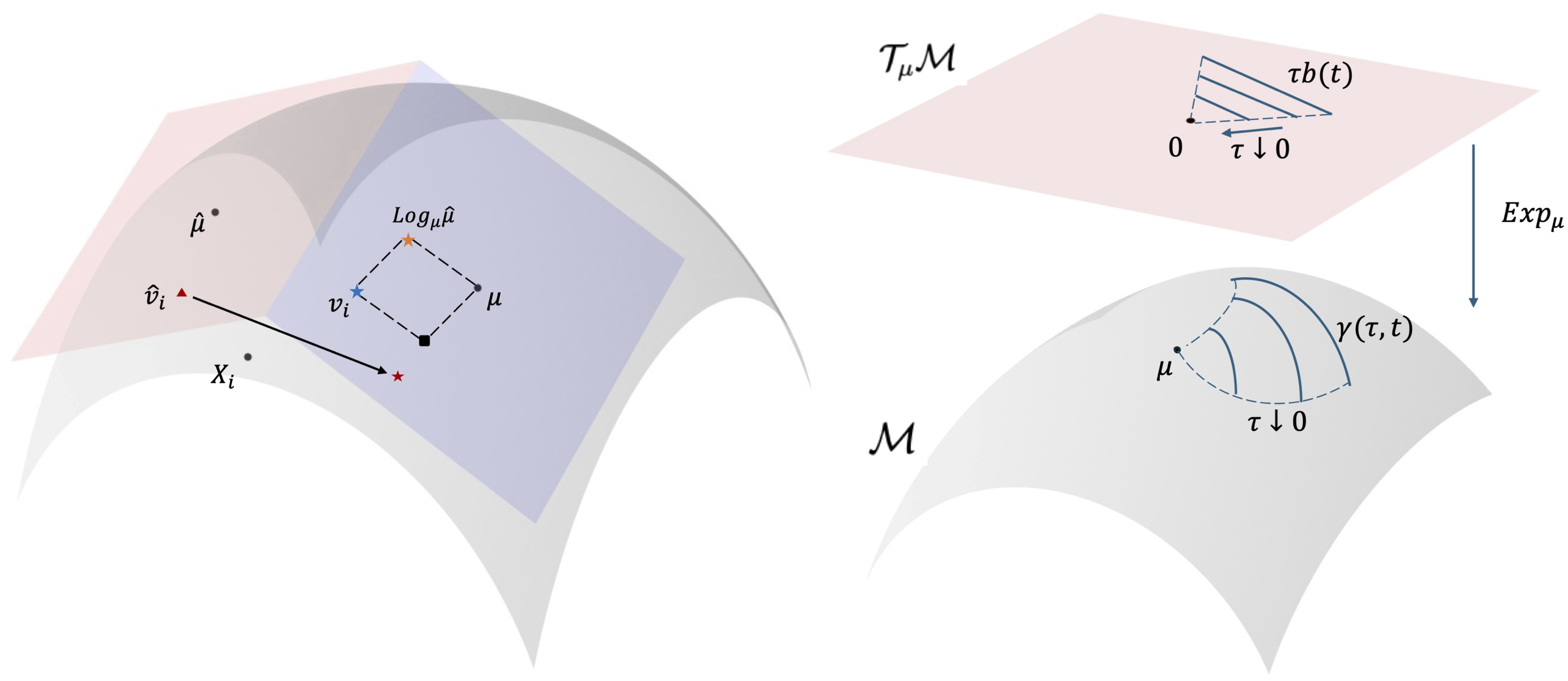
In Euclidean space and Hilbert space, the operator valued function is given by . In this case, we have and weakly converges to , which is identical to the convergence of the asymptotic distribution of as given in Zhou (2013). However, for a first-order stationary time series in a general Riemannian manifold with non-vanishing curvatures, , and the test proposed by Zhou (2013) is no longer valid since it does not include the additional term induced by the curvature. Intuitively, the difference between and is induced by the deviation shown in Figure 1, i.e., the deviations of from .
The limiting process established by Theorem 1 includes two components, specifically, a Gaussian random process with a complicated covariance function and a deterministic operator-valued function . To perform a valid test under null hypothesis, we propose to approximate the deterministic function by a CUSUM statistic and bootstrap the random process by adapting the Gaussian multiplier bootstrap in Zhou (2013). Specifically, for with some positive integer , we take as an estimate of . Roughly speaking, can be viewed as a plug-in estimate of by substituting with .
We bootstrap the Gaussian process by a moving-block multiplier bootstrap procedure, as follows. Let be a fixed block size. For each bootstrap sample, generate i.i.d standard Gaussian random variables . For with , define . Via resampling from , we can obtain an estimate of the null distribution of ; see Algorithm 1, where a test procedure is provided in Step 5. The following theorem establishes the consistency of the Gaussian multiplier bootstrap method with curvature term adjustment under the null, showing that the proposed test procedure is asymptotically valid.
Theorem 2
Suppose that the assumptions in Theorem 1 hold and the block-size satisfies , and . Under , conditioning on , we then have
| (4) |
Next we study the asymptotic local power of the proposed test, where we utilize tools of parametrized surfaces in manifolds (Do Carmo, 1992). Let be a constant, and be a smooth curve, be a parametrized surface near , and a collection of vector fields such that
-
•
For fixed , is a parallel orthonormal frame along ;
-
•
is smooth on for all .
We consider the following local alternative hypothesis under the locally stationary scheme:
| (5) |
for a locally stationary time series as in Definition 2 with
| (6) |
A visual illustration of this local alternative is provided Figure 1(b). This local alternative scheme possesses two properties. First, for each , the data is locally stationary associated with the mean curve and parallel orthonormal frame . Second, as , the time series smoothly changes and uniformly converges to a first-order stationary time series at a rate . In Euclidean space, this local alternative scheme is identical to the case where with for a smooth function and is a zero-mean locally stationary time series. The following theorems present the asymptotic results for the local alternative.
Theorem 3
Theorem 4
Theorem 4 suggests that, even under the local alternative, the bootstrap samples are asymp-totically drawn from the limiting null distribution, with some suitable block size that meets a stronger condition compared with those in Theorem 2. Theorems 3 and 4 together show that our method can detect the first-order non-stationarity with rate and has asymptotic power whenever and . Note that, in Theorem 3, if , i.e., under the null hypothesis, the asymptotic distribution of given by Eq.(7) is identical to the one in Theorem 2.
Remark 5
Our test for first-order stationarity differs from previous change point detection methods (Dubey & Müller, 2020; Wang et al., 2023; Jiang et al., 2024) by examining whether the mean is constant or varies (continuously or discontinuously) over time, allowing gradual changes. In contrast, their methods detect abrupt changes and assume the time series can be segmented into blocks of constant mean and variance, a condition not required in our test.
4.2 Second-order stationarity test
If a manifold time series is first-order stationary, it is natural to further test the second-order stationarity. Below we propose a second-order stationarity test for first-order stationary manifold time series using local spectral density (Dahlhaus, 1997; Dette et al., 2011; van Delft et al., 2021).
Let be a first-order stationary manifold time series with constant intrinsic mean . The local spectral density of the coordinate representation of under a given orthonormal frame , i.e., the time series , is , where we define throughout this paper. Under some technical assumptions introduced later, the local spectral density is well-defined. The second-order stationarity of is equivalent to a.e. on . Thus, testing the second-order stationarity is equivalent to testing the following hypothesis:
| (8) | ||||
We then define squared variation of by
where and is the Hilbert-Schmidt norm of complex matrices. Since Hilbert-Schmit norm is invariant under unitary transformation, is independent of choices of . Note that if and only if , . Thus, the testing the hypothesis in (8) is equivalent to testing
| (9) |
We adapt the technique from van Delft et al. (2021), initially created for assessing second-order stationarity in functional time series, into our context of manifold time series. Let and be two positive integers such that and is even. The intuition is to split the time series into blocks of size , and then estimate the local spectral density and the squared variation . Let be the empirical intrinsic mean and , where is the complex tensor product (i.e., conjugation included) and
Then the coordinate representation of under any orthonormal frame at can serve as an estimator of , and the test statistic is given by
where , , and .
To develop a test based on the statistic , we proceed with studying its asymptotic distribution. Let be a vector such that and
Given random variables , we denote the order joint cumulant of random variables by . We assume that satisfies the following conditions. For every even number , there exists a positive sequence such that, for all and for some , we have , and
-
(C1)
, for all ,
-
(C2)
, for all .
The conditions (C1) and (C2) are proposed to guarantee the existence of the local spectral density and the weak convergence of test statistics. Similar conditions are used in previous works (van Delft et al., 2021).
Theorem 5
Theorem 6
The above theorem implies that consistently estimates under . It also suggests that, for a significant level , we can conduct the test by rejecting the null hypothesis if , where is the quantile of standard normal distribution. Under , the quantity given by (10) also converges to in probability. Thus, when , the probability of rejecting the null hypothesis is approximately , where is the CDF of the standard normal distribution. This result implies that the test has asymptotic power as under any fixed alternative .
Interestingly, Theorem 5 implies that under certain regularity conditions, the null distribution of our test statistic for the second-order stationarity is not affected by the curvature. This is in contrast to the first-order stationarity test, where curvature does have an impact on the null distribution. The reason is that the curvature effect in is asymptotically neutralized by the curvature effect in under the null hypothesis. Under the alternative hypothesis, the curvature effect exists and asymptotically has a form of , where is an unknown deterministic vector in and vanishes when is Euclidean space. Thus, the asymptotic alternative distribution of is a Gaussian distribution, with a variance different from the one in Euclidean or Hilbert space. The asymptotic variance under the alternative is complex, and therefore not included here; details on the asymptotic behavior related to the curvature impact on the second-order stationarity test can be found in Section LABEL:s-proof:thm5 of the supplementary materials.
Remark 6
Our second-order stationarity test addresses a different setting from the variance change detection in non-Euclidean data proposed by Dubey & Müller (2020) and Jiang et al. (2024). Their focus is on detecting changes in , which, in our context, corresponds to testing whether the trace of the time-varying matrix remains independent of . In contrast, our test examines the entire variance structure, not just its trace, and also accommodates continuously varying variance over time.
Remark 7
Although the null distribution of the test statistic for the second-order stationarity on the manifold is the same as Hilbert space or Euclidean space, the block size is more restricted. For the test in Hilbert space, the upper bound of is of order (van Delft et al., 2021), while for the general manifold it is of order , since the curvature effect introduces a bias of order in non-trivial manifolds, as discussed in the supplementary materials.
Remark 8
The constant mean assumption is common in the literature on second-order stationarity tests (Dette et al., 2011; Preuß et al., 2013; van Delft et al., 2021), and when is non-constant but smooth, it can be estimated (van Delft et al., 2021). For instance, we can estimate using methods from Petersen & Müller (2019); Lin & Müller (2021), and then estimate by parallel transporting to along the estimated curve as a detrending procedure.
5 Simulations
In this section, we conduct Monte Carlo simulation experiments to study the finite sample performance of our proposed testing procedures in two cases: (i) hypersphere, a positively-curved manifold example; (ii) SPD-matrices endowed with negatively curved manifold structure.
5.1 Simulations for first-order stationarity test on spherical time series
In the numerical study of first-order stationarity test, we consider the following two settings, and report results for Type-I error rates under null and power under alternative hypothesis.
Setting (i): We simulate locally stationary time series on , as follows. Let for . Take be the geodesic such that and , and be a re-scaled version of for . We also denote the parallel transport map from to along the geodesic , which is equivalent to the parallel transport map from to along the geodesic in this simulation setting. For , let be the vector with at the and with at the other entries; we view as an orthonormal basis of . Then we consider the following time-varying auto-regressive models
| (11) |
where , if and if , , and is a parallel orthonormal frame along , i.e., . The parameter in Eq.(11) determines the deviation of the time series from first-order stationarity. When , the time series is first-order stationary. As increases, the model will deviate from the null and we use it to evaluate the performance of the test statistic under the alternative. In this setting, we consider .
Setting (ii): We next consider , the space of SPD matrices endowed with the affine-invariant metric (Moakher, 2005), which is a six-dimensional negatively-curved Riemannian manifold. Let be a geodesic joining and such that and , and define . Let be the set of symmetric matrices with at the and entries and at the remaining entries. Note that form an orthogonal basis of , with for , and for . Let be the parallel orthogonal frame along with initial value . We simulate the following time-varying auto-regressive process:
where , and the collection of are independent Gaussian random variables such that if and . Similarly, is the parallel transport map from to along the geodesic . When , the manifold time series is first-order stationary. For power study under alternative, we consider .
For the first-order stationary test in both scenarios, we consider . The number of Monte Carlo runs is . The null distribution of the test statistic is estimated by the curvature adjusted multiplier bootstrap (CAMB) method in Algorithm 1. We compare the proposed test against two approaches: (B1) a method that bootstrap , neglecting the curvature effect , and (B2) an approach that considers manifold time series as Euclidean multivariate time series, utilizing the multiplier bootstrap technique suggested by (Zhou, 2013), thereby overlooking the manifold structure. The bootstrap sample size is set as for all methods in this benchmark study.
The Type-I error rates of our method and the two comparison methods are reported in Table 1. In the sphere scenario, we find that the Type-I error rates of the two comparison methods are inflated, while our method controls the Type-I error well. In the context of SPD matrices, the first comparison method, B1, which overlooks the curvature, tends to be overly conservative in this instance, exhibiting an empirical rejection probability of approximately . This conservative approach may result in diminished power under the alternative hypothesis. Results of the comparison method B1 in both scenarios numerically support that the curvature term plays an important role in manifold time series. On the other hand, the second method, B2, which treats the data as Euclidean multivariate time series, leads to an escalation in the eigenvalues of the sample mean and variance. Consequently, the variance associated with the multiplier bootstrap also surges, rendering the Type-I error rates for this approach unreliable in this scenario.
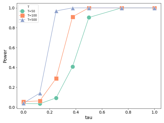
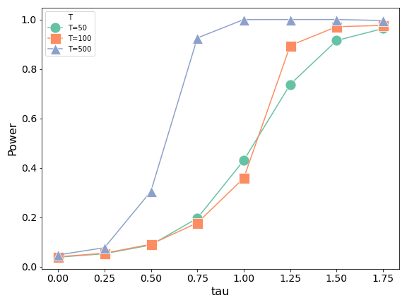
We also evaluate the power of the first-order stationary test by varying . For each fixed , the power is calculated based on repetitions of Monte Carlo runs. We plot the power curve in Figure 2, and as expected, one can observe that the test becomes more powerful as increases, and the power will ultimately reach as continues to increase.
5.2 Simulations for second-order stationarity test
To study the second-order stationarity test, for both and settings, we simulate locally stationary manifold time series which are first-order stationary from the model
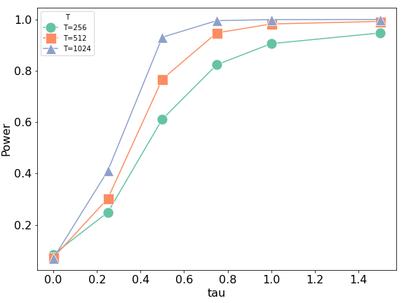
In the -dimensional hypersphere case, we set and take be an orthonormal basis of , as the in Setting (i) of Section 5.1. We set , and . For the -valued time series, is set to be , and is generated in the same way as Section 5.1. When , the manifold time series under both settings is second-order stationary, and when , the simulated time series is non-stationary in terms of the second order. We consider in the power study. We implement Monte Carlo replications with , respectively. The block size is set to be as suggested in van Delft et al. (2021).
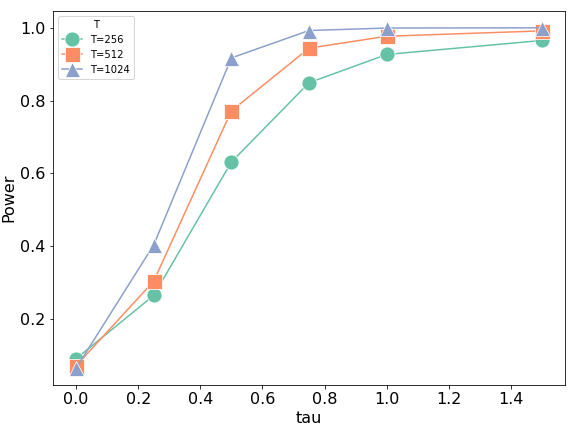
Type-I error rates are reported in Table 2. We observe that, under both and settings, at the significant level , the Type-I error rates decrease as increases, but are slightly inflated for relatively small . This slight inflation is due to an intrinsic limitation of the method we adapted (van Delft et al., 2021), which also applies to Euclidean time series. Specifically, we show in Table 2 that for an AR process in , the Type-I error rates of this testing procedure are also slightly larger than . In our power study, we observe that the testing power for both and settings increases to as grows; see Figure 3.
6 Application to Real Data
In this section, we apply our stationarity test to a single-cell RNA sequencing data generated by Schiebinger et al. (2019). The raw data is available at NCBI Gene Expression Omnibus (https://www.ncbi.nlm.nih.gov/geo/query/acc.cgi?acc=GSE122662). The goal is to understand the developmental process of mouse embryonic cells and model the change of cell-type proportion at each stage. To achieve this goal, scientists first obtained mouse embryonic cells from a single female embryo, plated cells for days, measured the gene expression profiles of cells collected across days, and finally profiled high-quality cells with variable genes after pre-processing. A nonlinear dimensionality reduction method called force-directed layout embedding (Jacomy et al., 2014) was used to visualize the temporal change of cellular populations in 2D in the original work, as shown in Figure 4. These cells were then assigned to seven major cell types by clustering and annotation with gene signature scores provided by prior biological knowledge. The annotated seven cell types are Mouse Embryonic Fibroblasts (MEFs), Mesenchymal-Epithelial Transition (MET) Cells, Induced Pluripotent Stem (IPS) Cells, Stromal Cells, Epithelial Cells, Neural Cells and Trophoblasts; each cell type has their own morphological features and functions. In this study, the proportions of these cell types are observed at each time point, with data collected at 37 time points over the course of 18 days (at 12-hour intervals).
A common approach to model the compositional data is the square-root transformation, which maps the data to a hypersphere. This transformation has an advantage that the composition constraint and zero components are naturally incorporated (Stephens, 1982; Scealy & Welsh, 2011). Applying square-root transformation to our data, we finally obtain a time series in hypersphere with length , with visualization provided in Figure 4. We aim to answer a biological question: does the cell-type proportion have systematic change over time, or equivalently, does the cell-type transition achieve dynamic equilibrium? This question is closely related to the discussion regarding validity of adopting a dynamic equilibrium assumption for modeling cellular dynamics without prior knowledge in cell biology (Schiebinger et al., 2019; Zhou et al., 2021; Sha et al., 2024). Statistically, the question is equivalent to testing the constancy of the mean of this hyperspherical time series , i.e., the first-order stationarity, and our proposed test serves as a tool to assess the feasibility of such an assumption when applied to real data.
Specifically, we apply the proposed first-order stationarity test to the data, with bootstrap sample size and block size selected by the minimum volatility method (Politis et al., 2012). The corresponding p-value is , providing a strong evidence to reject the null hypothesis. Thus, the cell-type proportions in this cell population undergo systematic temporal change, and cell-type transitions are still out of dynamic equilibrium. This result is consistent with the findings in Schiebinger et al. (2019), as they discovered that the extracted mouse embryonic cells have a strong ability of differentiation, and gradually moves to a terminal stromal state or a MET state, where the latter further generates pluripotent, extra-embryonic, and neural cells.
We then use the same dataset as an illustrative example to evaluate the proposed second-order stationarity test. In particular, we first estimate the mean curve using the total-variation regression with regularization parameters selected by leave-one-out cross validation (Lin & Müller, 2021). Then we parallelly transport from to along the as a detrend procedure, and apply the second-order test to the detrend version time-series . Since the sample size is small, we divide the data into overlapped blocks of size , which are and . The p-value associated to the second-order stationarity test is . The result shows that there is no significant evidence suggesting the uncertainty caused by the rate of random proliferation and apoptosis or noises due to technical issues in the sequencing platform varies over time. The constant uncertainty was implicitly made as an assumption of the biological model in Schiebinger et al. (2019) since the uncertainty parameter was shared by all time points in their models and numerical analysis, and our testing result provides a numerical support for the assumption in this dataset.
7 Discussion
In this paper, we introduce the definition of first-order and second-order stationarity of manifold-valued time series. We propose testing methods to test both first-order and second-order stationarity. Our methods can account for the curved nature of general manifolds. We derive the asymptotic consistency and asymptotic local powers of the tests. Numerical simulation studies and real data analysis are provided to illustrate the efficiency of our methods.
One limitation of our work is the dependency of our method for spectral density-based testing second-order stationarity on the choice of block size, a process that lacks a universally accepted benchmark and requires further improvement. This issue is not exclusive to our approach but is a widespread concern in the context of second-order stationarity assessments for time series within linear spaces (Dette et al., 2011; van Delft et al., 2021).
There are a few interesting future directions of our work. For example, in neuroscience study, an interesting question is how to detect structural break of dynamic functional connectivity Hutchison et al. (2013) when the state change. This issue can be approached as a problem of identifying breakpoints in manifold time series, which can be potentially solved by an extension of our framework to detect abrupt change in a block-wise locally stationary manifold time series. Another interesting extension is to generalize our framework and methods to the Wasserstein space , since can be viewed as an infinite-dimensional Hilbert manifold (Chen et al., 2023) by proper definition. However, an extension to general metric spaces is challenging and is still an open question, and we leave it for future research.
| T | CAMB | B1 | B2 | CAMB | B1 | B2 |
|---|---|---|---|---|---|---|
| 50 | 0.0364 | 0.0584 | 0.3936 | 0.0384 | 0.0082 | 0.0098 |
| 100 | 0.0544 | 0.1070 | 0.9806 | 0.0404 | 0.0086 | 0.0254 |
| 500 | 0.0392 | 0.1008 | 1.0000 | 0.0478 | 0.0098 | 0.1116 |
| T | |||
|---|---|---|---|
| 256 | 0.090 | 0.085 | 0.106 |
| 512 | 0.071 | 0.073 | 0.090 |
| 1024 | 0.064 | 0.070 | 0.074 |
Acknowledgment
We thank Robert J. McCann and Zhou Zhou for their insightful conversations and suggestions.
Supplementary Materials
The supplementary file contains technical proofs for the theorems in this article.
References
- (1)
- Aue & van Delft (2020) Aue, A. & van Delft, A. (2020), ‘Testing for stationarity of functional time series in the frequency domain’, The Annals of Statistics 48(5), 2505 – 2547.
- Bollerslev (1986) Bollerslev, T. (1986), ‘Generalized autoregressive conditional heteroskedasticity’, Journal of Econometrics 31(3), 307–327.
- Chen et al. (2023) Chen, Y., Lin, Z. & Müller, H.-G. (2023), ‘Wasserstein regression’, Journal of the American Statistical Association 118(542), 869–882.
- Dahlhaus (1997) Dahlhaus, R. (1997), ‘Fitting time series models to nonstationary processes’, The Annals of Statistics 25(1), 1–37.
- Dette et al. (2011) Dette, H., Preuß, P. & Vetter, M. (2011), ‘A measure of stationarity in locally stationary processes with applications to testing’, Journal of the American Statistical Association 106(495), 1113–1124.
- Do Carmo (1992) Do Carmo, M. P. (1992), Riemannian geometry, Vol. 6, Springer.
- Dubey & Müller (2020) Dubey, P. & Müller, H.-G. (2020), ‘Fréchet change-point detection’, The Annals of Statistics 48(6), 3312–3335.
- Fisher & Lee (1994) Fisher, N. I. & Lee, A. J. (1994), ‘Time series analysis of circular data’, Journal of the Royal Statistical Society. Series B (Methodological) 56(2), 327–339.
- Fréchet (1948) Fréchet, M. (1948), ‘Les éléments aléatoires de nature quelconque dans un espace distancié’, Annales de l’institut Henri Poincaré 10(4), 215–310.
- Hutchison et al. (2013) Hutchison, R. M., Womelsdorf, T., Allen, E. A., Bandettini, P. A., Calhoun, V. D., Corbetta, M., Della Penna, S., Duyn, J. H., Glover, G. H., Gonzalez-Castillo, J. et al. (2013), ‘Dynamic functional connectivity: promise, issues, and interpretations’, NeuroImage 80, 360–378.
- Jacomy et al. (2014) Jacomy, M., Venturini, T., Heymann, S. & Bastian, M. (2014), ‘Forceatlas2, a continuous graph layout algorithm for handy network visualization designed for the gephi software’, PLOS ONE 9(6), 1–12.
- Jiang et al. (2024) Jiang, F., Zhu, C. & Shao, X. (2024), ‘Two-sample and change-point inference for non-euclidean valued time series’, Electronic Journal of Statistics 18(1), 848–894.
- Lähnemann et al. (2020) Lähnemann, D., Köster, J., Szczurek, E., McCarthy, D. J., Hicks, S. C., Robinson, M. D., Vallejos, C. A., Campbell, K. R., Beerenwinkel, N., Mahfouz, A. et al. (2020), ‘Eleven grand challenges in single-cell data science’, Genome Biology 21(1), 1–35.
- Lin & Müller (2021) Lin, Z. & Müller, H.-G. (2021), ‘Total variation regularized Fréchet regression for metric-space valued data’, The Annals of Statistics 49(6), 3510 – 3533.
- Mardia et al. (2000) Mardia, K. V., Jupp, P. E. & Mardia, K. (2000), Directional statistics, Vol. 2, Wiley Online Library.
- Moakher (2005) Moakher, M. (2005), ‘A differential geometric approach to the geometric mean of symmetric positive-definite matrices’, SIAM Journal on Matrix Analysis and Applications 26(3), 735–747.
- Page (1954) Page, E. S. (1954), ‘Continuous inspection schemes’, Biometrika 41(1/2), 100–115.
- Pennec (2018) Pennec, X. (2018), ‘Barycentric subspace analysis on manifolds’, The Annals of Statistics 46(6A), 2711–2746.
- Petersen & Müller (2019) Petersen, A. & Müller, H.-G. (2019), ‘Fréchet regression for random objects with Euclidean predictors’, The Annals of Statistics 47(2), 691 – 719.
- Politis et al. (2012) Politis, D. N., Romano, J. P. & Wolf, M. (2012), Subsampling, Springer Science & Business Media.
- Preuß et al. (2013) Preuß, P., Vetter, M. & Dette, H. (2013), ‘A test for stationarity based on empirical processes’, Bernoulli 19(5B), 2715 – 2749.
- Priestley (1988) Priestley, M. B. (1988), ‘Non-linear and non-stationary time series analysis’, London: Academic Press .
- Scealy & Welsh (2011) Scealy, J. L. & Welsh, A. H. (2011), ‘Regression for compositional data by using distributions defined on the hypersphere’, Journal of the Royal Statistical Society. Series B: Statistical Methodology 73(3), 351–375.
- Schiebinger et al. (2019) Schiebinger, G., Shu, J., Tabaka, M., Cleary, B., Subramanian, V., Solomon, A., Gould, J., Liu, S., Lin, S., Berube, P. et al. (2019), ‘Optimal-transport analysis of single-cell gene expression identifies developmental trajectories in reprogramming’, Cell 176(4), 928–943.
- Sha et al. (2024) Sha, Y., Qiu, Y., Zhou, P. & Nie, Q. (2024), ‘Reconstructing growth and dynamic trajectories from single-cell transcriptomics data’, Nature Machine Intelligence 6(1), 25–39.
- Shao et al. (2022) Shao, L., Lin, Z. & Yao, F. (2022), ‘Intrinsic Riemannian functional data analysis for sparse longitudinal observations’, The Annals of Statistics 50(3), 1696 – 1721.
- Shumway et al. (2000) Shumway, R. H., Stoffer, D. S. & Stoffer, D. S. (2000), Time series analysis and its applications, Vol. 3, Springer.
- Stephens (1982) Stephens, M. A. (1982), ‘Use of the von mises distribution to analyse continuous proportions’, Biometrika 69(1), 197–203.
- van Delft & Blumberg (2024) van Delft, A. & Blumberg, A. J. (2024), ‘A statistical framework for analyzing shape in a time series of random geometric objects’.
- van Delft et al. (2021) van Delft, A., Characiejus, V. & Dette, H. (2021), ‘A nonparametric test for stationarity in functional time series’, Statistica Sinica 31(3), pp. 1375–1395.
- van Delft & Eichler (2018) van Delft, A. & Eichler, M. (2018), ‘Locally stationary functional time series’, Electronic Journal of Statistics 12(1), 107 – 170.
- Wang et al. (2023) Wang, X., Borsoi, R. A. & Richard, C. (2023), Online change point detection on riemannian manifolds with karcher mean estimates, in ‘2023 31st European Signal Processing Conference (EUSIPCO)’, IEEE, pp. 2033–2037.
- Wied et al. (2012) Wied, D., Krämer, W. & Dehling, H. (2012), ‘Testing for a change in correlation at an unknown point of time using an extended functional delta method’, Econometric Theory 28(3), 570–589.
- Wu (2005) Wu, W. B. (2005), ‘Nonlinear system theory: Another look at dependence’, Proceedings of the National Academy of Sciences 102(40), 14150–14154.
- Wu & Zhou (2011) Wu, W. B. & Zhou, Z. (2011), ‘Gaussian approximation for non-stationary multiple time series’, Statistica Sinica 21(3), 1397–1413.
- Yang et al. (2020) Yang, J., Gohel, S. & Vachha, B. (2020), ‘Current methods and new directions in resting state fMRI’, Clinical Imaging 65, 47–53.
- Zhou et al. (2021) Zhou, P., Wang, S., Li, T. & Nie, Q. (2021), ‘Dissecting transition cells from single-cell transcriptome data through multiscale stochastic dynamics’, Nature Communications 12(1), 5609.
- Zhou (2013) Zhou, Z. (2013), ‘Heteroscedasticity and autocorrelation robust structural change detection’, Journal of the American Statistical Association 108(502), 726–740.
- Zhou & Wu (2009) Zhou, Z. & Wu, W. B. (2009), ‘Local linear quantile estimation for nonstationary time series’, The Annals of Statistics pp. 2696–2729.
- Zhu & Müller (2024) Zhu, C. & Müller, H.-G. (2024), ‘Spherical autoregressive models, with application to distributional and compositional time series’, Journal of Econometrics 239(2), 105389.
See pages - of supp.pdf