Digital and Hybrid Precoding Designs in Massive MIMO with Low-Resolution ADCs

Abstract

Low-resolution analog-to-digital converters (ADCs) have emerged as an efficient solution for massive multiple-input multiple-output (MIMO) systems to reap high data rates with reasonable power consumption and hardware complexity. In this paper, we study precoding designs for digital, fully connected (FC) hybrid, and partially connected (PC) hybrid beamforming architectures in massive MIMO systems with low-resolution ADCs at the receiver. We aim to maximize the spectral efficiency (SE) subject to a transmit power budget and hardware constraints on the analog components. The resulting problems are nonconvex and the quantization distortion introduces additional challenges. To address them, we first derive a tight lower bound for the SE, based on which we optimize the precoders for the three beamforming architectures under the majorization-minorization framework. Numerical results validate the superiority of the proposed precoding designs over their state-of-the-art counterparts in systems with low-resolution ADCs, particularly those with 1-bit resolution. The results show that the PC hybrid precoding design can achieve an SE close to those of the digital and FC hybrid precoding designs in 1-bit systems, highlighting the potential of the PC hybrid beamforming architectures.

I Introduction

Massive multiple-input multiple-output (MIMO) technology is crucial for wireless communications at both sub-6 GHz and millimeter wave (mmWave) frequencies, addressing the increasing demand for high data rates [1]. The large number of antenna elements and the use of beamforming techniques significantly improve the spatial multiplexing gain and enable a high spectral efficiency (SE). However, a large number of power-hungry radio-frequency (RF) chains would cause high power consumption, degrading the system’s energy efficiency. In this respect, analog-to-digital converters (ADCs) are the most power-consuming RF components at the receiver, as their power consumption increases exponentially with the number of resolution bits [2]. Therefore, using low-resolution ADCs is considered to be an effective approach to reduce the power consumption without excessively compromising the SE performance [3]. However, the non-linear quantization distortion introduces additional challenges, calling for more efficient beamforming designs for achieving a satisfactory SE.

Existing precoding algorithms (e.g., [4, 5, 6, 7]) are mainly designed for digital beamforming (DBF) and hybrid beamforming (HBF) architectures. DBF architectures require a dedicated RF chain for each antenna, providing large spatial multiplexing gains at the expense of high power consumption. In contrast, HBF architectures employ fewer RF chains with a network of analog components, such as phase-shifters, to cut the hardware power consumption and cost at the expense of reduced spatial multiplexing. HBF implementations can be further divided into fully connected (FC) and partially connected (PC) HBF architectures (FC-HBF and PC-HBF). In the former, each RF chain can access all the antenna elements, while in the latter only a subset of the antenna elements is connected to each RF chain.

Traditional FC and PC hybrid precoding designs [4, 5, 6, 7] have predominantly focused on full-resolution systems, i.e, with high-resolution ADCs at the receiver. However, these designs tend to underperform in systems with low-resolution ADCs since they do not take the quantization distortion at the receiver into account. To address this challenge, existing studies [8, 9, 10, 11] have employed a heuristic two-step approach in which the analog precoder is optimized first and the digital precoder is determined second based on the analog design. For instance, Mo et. al. [8] derived the analog precoder based on the singular vectors of the channel, followed by the water-filling (WF) method to optimize the digital part. In [9], the analog precoder was chosen from a predefined codebook, after which the digital precoder was optimized to maximize the energy efficiency. Beyond HBF architectures, the quantization distortion also presents challenges for the digital precoding design. Conventional precoding strategies, including zero forcing, maximum ratio transmission, and minimum mean squared error, were explored in [12, 13, 14]. In [15], we jointly optimized the digital precoder and combiner, resulting in a substantial SE improvement over traditional WF solutions.

Despite the advances discussed above [8, 9, 10, 11, 12, 13, 14, 15], most studies have focused on only one of the three beamforming architectures: DBF, FC-HBF, or PC-HBF. Furthermore, HBF studies have often relied on heuristic methods for the analog precoding design, leaving considerable room for improving the SE. To fill this gap, we herein introduce a novel methodology that directly maximizes the SE and propose precoding designs for all the three architectures in systems with low-resolution ADCs at the receiver. Given the challenges posed by the hardware constraints at the transmitter and the quantization distortion at the receiver, we first derive a tight lower bound for the SE and then propose an iterative algorithm based on the majorization-minimization (MM) framework to optimize the precoders. Building on this, we develop efficient precoding designs for the DBF, FC-HBF, and PC-HBF architectures. Numerical results demonstrate that the proposed precoding designs outperform state-of-the-art methods [6, 4, 8, 15] in systems with low-resolution ADCs, particularly those with 1-bit resolution. Notably, our results indicate that the PC hybrid precoding design can achieve an SE close to those of the digital and FC hybrid precoding designs in 1-bit systems, highlighting the potential of PC-HBF architectures.

II System and Quantization Models

II-A MIMO Architecture Models

We consider a point-to-point narrowband MIMO system where a transmitter (Tx) with $N_{\rm t}$ antennas sends signals to a digital receiver (Rx) with $N_{\rm r}$ antennas, where the latter employs low-resolution ADCs. Let $\mathbf{s}\in{\mathbb{C}}^{N_{\rm s}}\sim\mathcal{C}\mathcal{N}(0,\mathbf{I})$ denote the transmitted signal vector and let $\mathbf{F}\in{\mathbb{C}}^{N_{\rm t}\times N_{\rm s}}$ be the precoding matrix with power constraint $\|\mathbf{F}\|_{\rm F}^{2}\leq P_{\rm t}$, where $P_{\rm t}$ denotes the transmit power budget and $\|\cdot\|_{\rm F}$ represents the Frobenius norm. For HBF architectures, $\mathbf{F}$ is given by $\mathbf{F}=\mathbf{F}_{\rm RF}\mathbf{F}_{\rm BB}$, where $\mathbf{F}_{\rm RF}\in{\mathbb{C}}^{N_{\rm t}\times N_{\rm RF}}$ and $\mathbf{F}_{\rm BB}\in{\mathbb{C}}^{N_{\rm RF}\times N_{\rm s}}$ are the analog and digital precoders, respectively, assuming $N_{\rm RF}$ RF chains ($N_{\rm s}\leq N_{\rm RF}\ll N_{\rm t}$). Each RF chain in the FC-HBF architecture is connected to all antennas through a network of phase shifters, while each RF chain in the PC-HBF architecture is connected only to a set of $M=\frac{N_{\rm t}}{N_{\rm RF}}$ antennas. For simplicity, we assume that $M$ is an integer and the $N_{\rm RF}$ groups of antennas are non-overlapping. Let $\mathcal{F}_{\rm full}$ and $\mathcal{F}_{\rm sub}$ denote the sets of feasible analog precoders for the FC-HBF and PC-HBF architectures, respectively, which can be expressed as

$$\mathcal{F}_{\rm full} =\{\mathbf{F}_{\rm RF}:|\mathbf{F}_{\rm RF}(i,j)|=1,~{}\forall i,j\},$$ (1)

$$\mathcal{F}_{\rm sub} =\big{\{}\mathbf{F}_{\rm RF}:\mathbf{F}_{\rm RF}={\rm blkdiag}\left(\mathbf{f}_{1},\ldots,\mathbf{f}_{\rm N_{\rm RF}}\right),$$

$$\hskip 56.9055pt\ \mathbf{f}_{n}\in{\mathbb{C}}^{M},|\mathbf{f}_{n}(i)|=1,~{}\forall,n,i\big{\}},$$ (2)

where $\mathbf{A}(i,j)$ and $\mathbf{a}(i)$ denote the ($i$,$j$)-th entry of $\mathbf{A}$ and the $i$-th element of $\mathbf{a}$, respectively.

Let $\mathbf{H}\in{\mathbb{C}}^{N_{\rm r}\times N_{\rm t}}$ be the channel between the Tx and Rx. The received signal can be expressed as

$$\mathbf{y}=\mathbf{H}\mathbf{F}\mathbf{s}+\mathbf{n},$$ (3)

where $\mathbf{n}\sim\mathcal{C}\mathcal{N}(0,\sigma_{\rm n}^{2}\mathbf{I})$ denotes an additive white Gaussian noise (AWGN) vector with power $\sigma_{\rm n}^{2}$. We assume that $\mathbf{H}$ is constant during each coherence time. In order to characterize the performance upper bound under our proposed scheme, we assume the availability of perfect channel state information at both the Tx and Rx [4, 5, 6, 7, 8, 9, 10, 11, 12, 13, 14, 15]. The quantization model is detailed next.

II-B Signal Model with Quantization

Assume that the ADCs are Llyod-Max quantizers [16] and that the Rx employs two identical ADCs in each RF chain to separately quantize the in-phase and quadrature signals. The codebook for a scalar quantizer of $b$ bits is defined as $\mathcal{C}=\{c_{0},\ldots,c_{N_{\rm q}-1}\}$, where $N_{\rm q}=2^{b}$ is the number of output levels of the quantizer. The set of quantization thresholds is $\mathcal{T}=\{t_{0},\ldots,t_{N_{\rm q}}\}$, where $t_{0}=-\infty$ and $t_{N_{\rm q}}=\infty$ allow inputs with arbitrary power. Let $Q(\cdot)$ denote the quantization function. For a complex signal $x=\Re\{x\}+j\Im\{x\}$, we have $Q(x)=Q\big{(}\Re\{x\}\big{)}+jQ\big{(}\Im\{x\}\big{)}$, with $Q\big{(}\Re\{x\}\big{)}=c_{i}$ when $\Re\{x\}\in[t_{i},t_{i+1}]$; the imaginary term $Q\big{(}\Im\{x\}\big{)}$ is obtained similarly. When the quantizer input is a vector, $Q(\cdot)$ is applied element-wise.

With fixed $\mathbf{H}$ and $\mathbf{F}$, we have $\mathbf{y}\sim\mathcal{C}\mathcal{N}(0,\mathbf{C}_{\mathbf{y}})$, where $\mathbf{C}_{\mathbf{y}}$ is the covariance matrix of $\mathbf{y}$, given by

$$\mathbf{C}_{\mathbf{y}}={\mathbb{E}}[\mathbf{y}\mathbf{y}^{\scriptscriptstyle\mathsf{H}}]=\mathbf{H}\mathbf{F}\mathbf{F}^{\scriptscriptstyle\mathsf{H}}\mathbf{H}^{\scriptscriptstyle\mathsf{H}}+\sigma_{\rm n}^{2}\mathbf{I}.$$ (4)

Let $\mathbf{z}=Q(\mathbf{y})$ be the quantization of $\mathbf{y}$. Using the Bussgang decomposition [17], we can write

$$\mathbf{z}=\mathbf{G}\mathbf{y}+{\bm{\eta}},$$ (5)

where $\mathbf{G}$ and ${\bm{\eta}}$ represent the Bussgang gain matrix and the quantization distortion vector, respectively. Furthermore, $\mathbf{G}$ can be expressed as $\mathbf{G}=\mathbf{I}-{\bm{\Gamma}}$, with ${\bm{\Gamma}}={\rm diag}(\gamma_{1},\cdots,\gamma_{N_{\rm r}})$. Here, $\gamma_{i}$ denotes the distortion factor of the ADCs for the $i$-th RF chain, which depends on the number of resolution bits as $\gamma(b)\approx 2^{-1.74b+0.28}$ [15]. Combined with (3), (5) can be rewritten as

$$\mathbf{z}=\mathbf{G}\mathbf{H}\mathbf{F}\mathbf{s}+\mathbf{e},$$ (6)

where $\mathbf{e}=\mathbf{G}\mathbf{n}+{\bm{\eta}}$ represents the effective noise, which is not Gaussian due to the non-linear quantization distortion.

III Digital and Hybrid Precoding Designs

III-A Problem Formulation

Treating the effective noise $\mathbf{e}$ as Gaussian, we can obtain a lower bound for the SE as [8, 15]

$$R=\log\det\left(\mathbf{I}+\mathbf{C}_{\mathbf{e}}^{-1}\mathbf{G}\mathbf{H}\mathbf{F}\mathbf{F}^{\scriptscriptstyle\mathsf{H}}\mathbf{H}^{\scriptscriptstyle\mathsf{H}}\mathbf{G}\right),$$ (7)

where the covariance matrix of $\mathbf{e}$ is given by $\mathbf{C}_{\mathbf{e}}={\mathbb{E}}[\mathbf{e}\mathbf{e}^{\scriptscriptstyle\mathsf{H}}]=\mathbf{C}_{{\bm{\eta}}}+\sigma_{\rm n}^{2}\mathbf{G}^{2}$. Here, $\mathbf{C}_{{\bm{\eta}}}={\mathbb{E}}[{\bm{\eta}}{\bm{\eta}}^{\scriptscriptstyle\mathsf{H}}]$ is the covariance of the quantization distortion, which can be approximated as $\mathbf{C}_{{\bm{\eta}}}\approx\mathbf{G}\left(\mathbf{I}-\mathbf{G}\right){\rm diag}(\mathbf{C}_{\mathbf{y}})$ [15]. Thus, we obtain

$$\mathbf{C}_{\mathbf{e}}\approx\mathbf{G}\left(\mathbf{I}-\mathbf{G}\right){\rm diag}\left(\mathbf{H}\mathbf{F}\mathbf{F}^{\scriptscriptstyle\mathsf{H}}\mathbf{H}^{\scriptscriptstyle\mathsf{H}}\right)+\sigma_{\rm n}^{2}\mathbf{G}.$$ (8)

We are interested in optimizing the precoder $\mathbf{F}$ to maximize the SE in (7), i.e.,

$$\underset{\|\mathbf{F}\|^{2}_{F}\leq P_{\rm t}}{\mathrm{maximize}}\;R(\mathbf{F}).$$ (9)

For HBF architectures, the additional constraints

$$\mathbf{F}=\mathbf{F}_{\rm RF}\mathbf{F}_{\rm BB},$$ (10)

$$\mathbf{F}_{\rm RF}\in\mathcal{F}$$ (11)

must be satisfied, where $\mathcal{F}=\mathcal{F}_{\rm full}$ for FC-HBF and $\mathcal{F}=\mathcal{F}_{\rm sub}$ for PC-HBF. Problem (9) is nonconvex and more challenging compared with conventional precoding designs in full-resolution systems because $\mathbf{C}_{\mathbf{e}}$ depends on $\mathbf{F}$ through (8). To overcome this difficulty, we propose an efficient iterative algorithm based on the MM framework. To make the problem more tractable, we first derive a tight lower bound for $R(\mathbf{F})$ in the following lemma.

Lemma 1

Let $\hat{\mathbf{F}}$ be a prior estimate of $\mathbf{F}$ and define $\mathbf{X}=\mathbf{G}\mathbf{H}\mathbf{F}$. Furthermore, let

$$g(\mathbf{F},\hat{\mathbf{F}}) =R(\hat{\mathbf{F}})-{\rm Tr}(\hat{\mathbf{X}}^{\scriptscriptstyle\mathsf{H}}\hat{\mathbf{C}}_{\mathbf{e}}^{-1}\hat{\mathbf{X}})+2\Re\big{\{}{\rm Tr}(\hat{\mathbf{X}}^{\scriptscriptstyle\mathsf{H}}\hat{\mathbf{C}}_{\mathbf{e}}^{-1}\mathbf{X})\big{\}}$$

$$\hskip 85.35826pt-{\rm Tr}\big{\{}\hat{\mathbf{S}}(\mathbf{C}_{\mathbf{e}}+\mathbf{X}\mathbf{X}^{\scriptscriptstyle\mathsf{H}})\big{\}},$$ (12)

where $\hat{\mathbf{X}}$ and $\hat{\mathbf{C}}_{\mathbf{e}}$ are obtained based on $\hat{\mathbf{F}}$, and $\hat{\mathbf{S}}=\hat{\mathbf{C}}_{\mathbf{e}}^{-1}-(\hat{\mathbf{C}}_{\mathbf{e}}+\hat{\mathbf{X}}\hat{\mathbf{X}}^{\scriptscriptstyle\mathsf{H}})^{-1}$. Note that $g(\mathbf{F},\hat{\mathbf{F}})$ depends on $\mathbf{F}$ and $\hat{\mathbf{F}}$ through $\{\mathbf{X},\mathbf{C}_{\mathbf{e}}\}$ and $\{\hat{\mathbf{X}},\hat{\mathbf{C}}_{\mathbf{e}}\}$, respectively. It can be shown that $g(\mathbf{F},\hat{\mathbf{F}})$ is a tight lower bound for $R(\mathbf{F})$, i.e., $g(\mathbf{F},\hat{\mathbf{F}})\leq R(\mathbf{F})$, where the equality holds only if $\hat{\mathbf{F}}=\mathbf{F}$.

Lemma 1 is obtained based on [18, Proposition 7]; the proof is omitted due to space limitations. Using Lemma 1, we can update $\mathbf{F}$ by iteratively maximizing $g(\mathbf{F},\hat{\mathbf{F}})$ using the MM framework. Next, we use this method to propose efficient solutions for digital and hybrid precoding.

III-B Digital Precoding Design

Let $p_{i}^{2}$ be the power allocated to the $i$-th data stream, and let $\mathbf{p}=[p_{1},\ldots,p_{N_{\rm s}}]^{\scriptscriptstyle\mathsf{T}}$. Furthermore, let $\mathbf{H}=\mathbf{U}{\bm{\Sigma}}\mathbf{V}^{\scriptscriptstyle\mathsf{H}}$ be the singular value decomposition (SVD) of $\mathbf{H}$. The precoder can be constructed as

$$\mathbf{F}=\tilde{\mathbf{V}}{\rm diag}(\mathbf{p}),$$ (13)

where $\tilde{\mathbf{V}}=\mathbf{V}(:,1:N_{\rm s})$ contains the $N_{\rm s}$ right-singular vectors associated with the $N_{\rm s}$ largest singular values of $\mathbf{H}$. As a result, the precoding design becomes the power allocation problem $\mathrm{maximize}_{\|\mathbf{p}\|^{2}\leq P_{\rm t}}\,g(\mathbf{p},\hat{\mathbf{p}})$ that follows from Lemma 1. After some algebraic manipulations, we obtain the equivalent problem

$$\underset{\mathbf{p}}{\mathrm{minimize}} \quad\sum_{i=1}^{N_{\rm s}}\hat{\mathbf{J}}(i,i)p_{i}^{2}-2\sum_{i=1}^{N_{\rm s}}\Re\big{\{}\hat{\mathbf{K}}(i,i)p_{i}\big{\}}$$ (14a)

$$\mathrm{s.t.}\hskip 11.38109pt \quad\sum_{i=1}^{N_{\rm s}}p_{i}^{2}\leq P_{\rm t},$$ (14b)

where $\hat{\mathbf{J}}=\tilde{\mathbf{V}}^{\scriptscriptstyle\mathsf{H}}\mathbf{H}^{\scriptscriptstyle\mathsf{H}}\big{(}\mathbf{G}\hat{\mathbf{S}}\mathbf{G}+{\rm diag}(\hat{\mathbf{S}})\mathbf{G}(\mathbf{I}-\mathbf{G})\big{)}\mathbf{H}\tilde{\mathbf{V}}$, $\hat{\mathbf{K}}={\rm diag}(\hat{\mathbf{p}}^{\frac{1}{2}})\tilde{\mathbf{V}}^{\scriptscriptstyle\mathsf{H}}\mathbf{H}^{\scriptscriptstyle\mathsf{H}}\mathbf{G}\hat{\mathbf{C}}_{\mathbf{e}}^{-1}\mathbf{G}\mathbf{H}\tilde{\mathbf{V}}{\rm diag}(\hat{\mathbf{p}}^{\frac{1}{2}})$, and $\mathbf{a}^{\frac{1}{2}}$ is obtained by taking the element-wise square root of the elelemts of $\mathbf{a}$. Setting the derivative of the Lagrangian of (14) to zero, we obtain the solution as

$$p_{i}=\frac{\hat{\mathbf{K}}(i,i)}{\hat{\mathbf{J}}(i,i)+\mu}\quad\forall i\,,$$ (15)

where $\mu$ is the associated Lagrange multiplier, which can be obtained via a bisection search over $(0,\mu_{\rm ub}]$ to satisfy $\sum_{i=1}^{N_{\rm s}}p_{i}^{2}=P_{\rm t}$, where $\mu_{\rm up}=\frac{1}{\sqrt{P_{\rm t}}}\big{\|}{\rm diag}(\hat{\mathbf{K}})\big{\|}_{\rm F}$ is obtained by letting $\hat{\mathbf{J}}=\mathbf{0}$.

The proposed digital precoding design is summarized in Algorithm 1. We note that the conventional WF solution, denoted by $\mathbf{F}_{\rm WF}$, is obtained by assuming $\mathbf{C}_{{\bm{\eta}}}=\mathbf{0}$ as in full-resolution systems. Hence, $\mathbf{F}_{\rm WF}$ is sub-optimal for (14) due to the presence of the quantization distortion, as will be shown in Section IV.

Output: $\mathbf{F}$

1 Initialize $\mathbf{p},\epsilon$.

2 Perform SVD $\mathbf{H}=\mathbf{U}{\bm{\Sigma}}\mathbf{V}^{\scriptscriptstyle\mathsf{H}}$ and set $\tilde{\mathbf{V}}=\mathbf{V}(:,1:N_{\rm s})$.

3 repeat

4       $\hat{\mathbf{p}}\leftarrow\mathbf{p}$.

5       Update $\mathbf{p}$ as in (15).

6      

7until  $\left|R(\mathbf{p})-R(\hat{\mathbf{p}})\right|\leq\epsilon$;

Obtain $\mathbf{F}$ by (13).

Algorithm 1 MM-based Digital Precoding Design

III-C Hybrid Precoding Design

Define $f(\mathbf{F}_{\rm RF},\mathbf{F}_{\rm BB})={\rm Tr}(\hat{\mathbf{L}}\mathbf{F}_{\rm RF}\mathbf{F}_{\rm BB}\mathbf{F}_{\rm BB}^{\scriptscriptstyle\mathsf{H}}\mathbf{F}_{\rm RF}^{\scriptscriptstyle\mathsf{H}})-2\Re\big{\{}{\rm Tr}(\hat{\mathbf{D}}\mathbf{F}_{\rm RF}\mathbf{F}_{\rm BB})\big{\}}$ with $\hat{\mathbf{D}}=\hat{\mathbf{X}}^{\scriptscriptstyle\mathsf{H}}\hat{\mathbf{C}}_{\mathbf{e}}^{-1}\mathbf{G}\mathbf{H}$ and $\hat{\mathbf{L}}=\mathbf{H}^{\scriptscriptstyle\mathsf{H}}\big{(}{\rm diag}(\hat{\mathbf{S}})\mathbf{G}(\mathbf{I}-\mathbf{G})+\mathbf{G}\hat{\mathbf{S}}\mathbf{G}\big{)}\mathbf{H}$. Using Lemma 1, the subproblem for the hybrid precoding design in each iteration is expressed as

$$\underset{\mathbf{F},\mathbf{F}_{\rm RF},\mathbf{F}_{\rm BB}}{\mathrm{minimize}}\; f(\mathbf{F}_{\rm RF},\mathbf{F}_{\rm BB})$$ (16a)

$$\mathrm{s.t.}\hskip 17.07164pt \text{ \eqref{eq: coupling constraints} and \eqref{eq: analog components}},$$

$$\|\mathbf{F}\|_{\rm F}^{2}\leq P_{\rm t},$$ (16b)

which is challenging due to the constraints (10) and (11). Observing that $f(\mathbf{F}_{\rm RF},\mathbf{F}_{\rm BB})$ is convex with respect to $\mathbf{F}_{\rm RF}$ ($\mathbf{F}_{\rm BB}$) when $\mathbf{F}_{\rm BB}$ ($\mathbf{F}_{\rm RF}$) is fixed, we compute the analog and digital precoders via alternating optimization, as explained next.

III-C1 Update $\mathbf{F}_{\rm RF}$

For a given $\mathbf{F}_{\rm BB}$, the problem of designing $\mathbf{F}_{\rm RF}$ can be written as $\mathrm{minimize}_{\mathbf{F}_{\rm RF}\in\mathcal{F}}\;f(\mathbf{F}_{\rm RF},\mathbf{F}_{\rm BB})$, with $\mathcal{F}=\mathcal{F}_{\rm full}$ for FC-HBF and $\mathcal{F}=\mathcal{F}_{\rm sub}$ for PC-HBF. To efficiently solve this problem, we propose to use the projected gradient descent (PGD) method. Specifically, let $\nabla_{\mathbf{F}_{\rm RF}}f$ denote the gradient of $f(\mathbf{F}_{\rm RF},\mathbf{F}_{\rm BB})$ with respect to $\mathbf{F}_{\rm RF}$, given by

$$\nabla_{\mathbf{F}_{\rm RF}}f=2(\hat{\mathbf{L}}\mathbf{F}_{\rm RF}\mathbf{F}_{\rm BB}-\hat{\mathbf{D}}^{\scriptscriptstyle\mathsf{H}})\mathbf{F}_{\rm BB}^{\scriptscriptstyle\mathsf{H}},$$ (17)

and let ${\rm Proj}_{\mathcal{F}}(\mathbf{F}_{\rm RF})$ represent the operation that projects $\mathbf{F}_{\rm RF}$ onto $\mathcal{F}$. Define $\mathbf{W}={\rm blkdiag}(\mathbf{1}_{M},\ldots,\mathbf{1}_{M})$, where $\mathbf{1}_{M}\in{\mathbb{R}}^{M}$ is the $M$-dimensional all-one vector. The projectors for FC-HBF and PC-HBF are given by

$${\rm Proj}_{\mathcal{F}_{\rm full}}(\mathbf{F}_{\rm RF})=e^{j\angle\mathbf{F}_{\rm RF}},$$ (18a)

$${\rm Proj}_{\mathcal{F}_{\rm sub}}(\mathbf{F}_{\rm RF})=\mathbf{W}\odot e^{j\angle\mathbf{F}_{\rm RF}},$$ (18b)

respectively, where $\angle\mathbf{F}_{\rm RF}$ returns the angles of each entry of $\mathbf{F}_{\rm RF}$ and $\odot$ denotes the Hadamard product. The update rules for the PGD method can be expressed as

$$\mathbf{F}_{\rm RF}\leftarrow{\rm Proj}_{\mathcal{F}}\left(\tilde{\mathbf{F}}_{\rm RF}-\beta\frac{\nabla_{\mathbf{F}_{\rm RF}}f}{\|\nabla_{\mathbf{F}_{\rm RF}}f\|_{\rm F}}\bigg{|}_{\mathbf{F}_{\rm RF}=\tilde{\mathbf{F}}_{\rm RF}}\right),$$ (19)

where $\beta$ denotes the step size and $\tilde{\mathbf{F}}_{\rm RF}$ is the iterate of $\mathbf{F}_{\rm RF}$. The detailed steps for obtaining $\mathbf{F}_{\rm RF}$ are similar to those in [19, Algorithm 1] and are thus omitted.

III-C2 Update $\mathbf{F}_{\rm BB}$

For a given $\mathbf{F}_{\rm RF}$, we can obtain a closed-form solution for $\mathbf{F}_{\rm BB}$ as

$$\mathbf{F}_{\rm BB}=(\mathbf{F}_{\rm RF}^{\scriptscriptstyle\mathsf{H}}\hat{\mathbf{L}}\mathbf{F}_{\rm RF}+\lambda\mathbf{F}_{\rm RF}^{\scriptscriptstyle\mathsf{H}}\mathbf{F}_{\rm RF})^{-1}\mathbf{F}_{\rm RF}^{\scriptscriptstyle\mathsf{H}}\hat{\mathbf{D}}^{\scriptscriptstyle\mathsf{H}},$$ (20)

where $\lambda$ is the Lagrange multiplier associated with the power constrain, and can be obtained via a bisection search over $(0,\lambda_{\rm ub}]$, with $\lambda_{\rm ub}=\frac{1}{\sqrt{P_{\rm t}}}\|\left(\mathbf{F}_{\rm RF}^{\scriptscriptstyle\mathsf{H}}\mathbf{F}_{\rm RF}\right)^{-\frac{1}{2}}\mathbf{F}_{\rm RF}^{\scriptscriptstyle\mathsf{H}}\hat{\mathbf{D}}^{\scriptscriptstyle\mathsf{H}}\|_{\rm F}$, based on the complementary slackness condition $\lambda\left({\rm Tr}\left(\mathbf{F}_{\rm RF}^{\scriptscriptstyle\mathsf{H}}\mathbf{F}_{\rm RF}\mathbf{F}_{\rm BB}\mathbf{F}_{\rm BB}^{\scriptscriptstyle\mathsf{H}}\right)-P_{\rm t}\right)=0$.

The proposed hybrid precoding design is summarized in Algorithm 2. The precoder $\mathbf{F}$ is initialized with the conventional WF precoder $\mathbf{F}_{\rm WF}$. Let $\mathbf{V}_{\rm a}=\mathbf{V}(:,1:N_{\rm RF})$ contain the $N_{\rm RF}$ singular vectors associated with the $N_{\rm RF}$ largest singular values of $\mathbf{H}$. We initialize $\mathbf{F}_{\rm RF}=\mathbf{V}_{\rm a}$ for FC-HBF or $\mathbf{F}_{\rm RF}=\mathbf{W}\odot\mathbf{V}_{\rm a}$ for PC-HBF, which yields $\mathbf{F}_{\rm BB}=\mathbf{F}_{\rm RF}^{\dagger}\mathbf{F}_{\rm WF}$. Algorithms 1 and 2 are guaranteed to converge according to the MM theory.

Output: $\mathbf{F}_{\rm RF},\mathbf{F}_{\rm BB}$

1 Initialize $\mathbf{F}_{\rm RF}\in\mathcal{F},\mathbf{F}$, $\mathbf{F}_{\rm BB}=\mathbf{F}_{\rm RF}^{\dagger}\mathbf{F},\epsilon$.

2 repeat

3       $\hat{\mathbf{F}}\leftarrow\mathbf{F}$ .

4       repeat

5             Update $\mathbf{F}_{\rm RF}$ via the PGD method.

6             Update $\mathbf{F}_{\rm BB}$ as in (20).

7      until $f(\mathbf{F}_{\rm RF},\mathbf{F}_{\rm BB})$ stops decreasing;

8      $\mathbf{F}=\mathbf{F}_{\rm RF}\mathbf{F}_{\rm BB}$.

9until  $\left|R(\mathbf{F})-R(\hat{\mathbf{F}})\right|\leq\epsilon$;

Algorithm 2 MM-based Hybrid Precoding Design

III-D Complexity Analysis

Let $I_{1}$ be the number of iterations for Algorithm 1. With $N_{\rm s}\ll\min(N_{\rm r},N_{\rm t})$, the complexity of Algorithm 1 can be expressed as $I_{1}\mathcal{O}\left(2N_{\rm r}^{2}N_{\rm t}+2N_{\rm r}^{3}+4N_{\rm r}^{2}N_{\rm s}+6N_{\rm r}N_{\rm t}N_{\rm s}\right)$ floating-point operations (FLOPs) due mainly to matrix multiplications and inverses. For Algorithm 2, step 5 has a complexity of $\mathcal{O}(I_{\rm pgd}N_{\rm t}^{2}N_{\rm RF})$ due to the matrix multiplication, where $I_{\rm pgd}$ denotes the number of PGD iterations, whereas computing $\mathbf{F}_{\rm BB}$ in step 6 requires $\mathcal{O}(N_{\rm t}^{2}N_{\rm RF})$ FLOPs. Furthermore, $\hat{\mathbf{X}}$, $\hat{\mathbf{C}}_{\mathbf{e}}$, $\hat{\mathbf{L}}$, and $\hat{\mathbf{D}}$ are computed in the outer loop, requiring $\mathcal{O}\left(2N_{\rm r}^{2}N_{\rm t}+2N_{\rm r}^{3}+6N_{\rm r}^{2}N_{\rm RF}+5N_{\rm r}N_{\rm t}N_{\rm RF}\right)$ FLOPs. Therefore, the complexity of Algorithm 2 can be expressed as $I_{\rm out}N_{\rm RF}\mathcal{O}\left(6N_{\rm r}^{2}+5N_{\rm r}N_{\rm t}+I_{\rm in}I_{\rm pgd}N_{\rm t}^{2}\right)+I_{\rm out}\mathcal{O}\left(2N_{\rm r}^{2}N_{\rm t}+2N_{\rm r}^{3}\right)$, where $I_{\rm in}$ and $I_{\rm out}$ denote, respectively, the number of iterations for the inner and outer loops of Algorithm 2.

The complexity of the proposed algorithms is summarized and compared with that in [8, 4, 6, 15] in Table I. Algorithm 1 has a lower complexity than the digital precoding design in [15], as the former focuses only on precoding. Algorithm 2 has a higher complexity compared with the algorithms in [8, 4, 6] due to the optimization of the hybrid precoders to directly maximize the SE. However, the proposed digital precoding design can achieve an SE comparable to that of [15], and the proposed hybrid precoding designs can attain higher SE in low-resolution systems, as illustrated next.

IV Numerical Results

In all simulations, we assume that the system operates at $28$ GHz with bandwidth of $1$ GHz. We employ the Saleh-Valenzuela channel model and configure the channel parameters as those in [4]. The signal-to-noise ratio (SNR) is defined as SNR$~{}=\frac{P_{\rm t}}{\sigma_{\rm n}^{2}}$ and we assume identical $b$-bit ADCs for each RF chain. The other parameters are detailed in the caption of each figure. All the results are obtained by averaging over $10^{3}$ independent channel realizations.

For comparison, we consider the following baselines:

• “UqOpt”: Using $\mathbf{F}_{\rm WF}$ for maximizing the SE with full-resolution ADCs.

• “DBF: WF”: Using $\mathbf{F}_{\rm WF}$ with low-resolution ADCs.

• “DBF: JPC”: Joint design of digital precoder and combiner for low-resolution ADCs [15].

• “FC-HBF: SVD-based”: SVD-based FC hybrid precoding with low-resolution ADCs [8].

• “FC-HBF: AO”: FC hybrid precoding design with full-resolution systems [4].

• “PC-HBF: SVD-based”: Modified SVD-based design [8] with projection of the analog precoder onto $\mathcal{F}_{\rm sub}$.

• “PC-HBF: SIC”: PC hybrid precoding design with full-resolution systems [6].

Additionally, the SE of all the precoding schemes is based on the simulated $\mathbf{C}_{{\bm{\eta}}}$ for a more practical performance characterization (rather than on the diagonal approximation in (8)). The simulated $\mathbf{C}_{{\bm{\eta}}}$ is obtained using a sample average over $10^{5}$ realizations.

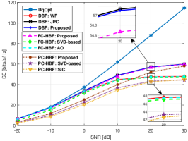
(a) SE versus SNR ($b=3$).

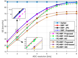
(b) SE versus ADC resolution ($\textrm{SNR}=20$ dB).

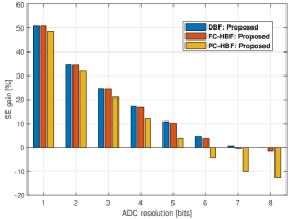
(c) SE gain versus ADC resolution ($\textrm{SNR}=30$ dB).

Figure 1: SE performance ($N_{\rm t}=N_{\rm r}=64$ and $N_{\rm s}=N_{\rm RF}=8$).

Algorithm	Computational complexity
Algorithm 1	$I_{1}\mathcal{O}\left(2N_{\rm r}^{2}N_{\rm t}+2N_{\rm r}^{3}+4N_{\rm r}^{2}N_{\rm s}+6N_{\rm r}N_{\rm t}N_{\rm s}\right)$
DBF [15]	$I_{\rm n}\mathcal{O}(3N_{\rm t}^{3}+3N_{\rm t}^{3}+8N_{\rm t}^{2}N_{\rm r}+8N_{\rm t}N_{\rm r}^{2})$
Algorithm 2	$I_{\rm out}N_{\rm RF}\mathcal{O}\left(6N_{\rm r}^{2}+5N_{\rm r}N_{\rm t}+I_{\rm in}I_{\rm pgd}N_{\rm t}^{2}\right)$ $+I_{\rm out}\mathcal{O}\left(2N_{\rm r}^{2}N_{\rm t}+2N_{\rm r}^{3}\right)$
FC-HBF [8]	$\mathcal{O}(N_{\rm t}N_{\rm r}N_{\rm RF}+I_{\rm c}N_{\rm t}N_{\rm RF}^{2}+2I_{\rm c}N_{\rm RF}^{3})$
FC-HBF [4]	$I_{\rm o}\mathcal{O}\left(2N_{\rm t}N_{\rm RF}^{2}+I_{\rm i}N_{\rm t}^{2}N_{\rm RF}\right)$
PC-HBF [6]	$\mathcal{O}\left(N_{\rm r}^{3}N_{\rm RF}+N_{\rm r}^{2}N_{\rm t}N_{\rm RF}+N_{\rm t}^{2}N_{\rm r}N_{\rm RF}\right)$

TABLE I: Computational complexity of the considered algorithms. Here, $I_{\rm n}$ and $I_{\rm c}$ denote the number of iterations of the designs in [15] and [8], respectively, while $I_{\rm o}$ and $I_{\rm i}$ represent the number of iterations of the outer and inner loop for the method in [4].

In Figs. 1(a) and 1(b), we plot the SE versus the SNR and ADC resolution, respectively, with $N_{\rm t}=N_{\rm r}=64$ and $N_{\rm s}=N_{\rm RF}=8$. From Fig. 1(a), we observe that the proposed digital precoding design achieves an SE comparable to that of the “DBF: JPC”. Furthermore, the proposed FC-HBF and PC-HBF schemes outperform their benchmark counterparts and perform better at high SNR. For example, at $\textrm{SNR}=20$ dB, the proposed FC-HBF and PC-HBF approaches achieve $19\%$ and $21\%$ improvements in SE over the “FC-HBF: AO” and ‘PC-HBF: SVD-based”, respectively. Additionally, it is seen that both the proposed FC and PC hybrid precoding designs outperform WF-based digital precoding in low-resolution systems at high SNR. In particular, the proposed FC hybrid precoding design attains SE comparable to that of the proposed digital one. Fig. 1(b) shows that the proposed DBF, FC-HBF, and PC-HBF schemes achieve significantly higher SE compared with their benchmarks, especially for low ADC resolutions. Notably, PC-HBF achieves an SE comparable to those of DBF and FC-HBF as the ADC resolution decreases. This is further illustrated in Fig. 1(c), which shows the SE gain in $\%$ of DBF, FC-HBF, and PC-HBF compared with the WF-based digital precoding design. The proposed precoding designs achieve $51\%$, $51\%$, and $49\%$ SE gains with 1-bit ADCs. However, when $b\geq 8$, PC-HBF achieves lower SE than WF-based DBF.

In Fig. 2, we plot the SE as a function of the number of data streams with $N_{\rm r}=N_{\rm t}=64$, $\textrm{SNR}=20$ dB, and $b=3$. It is seen that the SE gains of the proposed methods are more significant with more data streams. While for $N_{\rm s}\leq 4$ the SE difference between the proposed precoding design and the benchmark algorithms is relatively small, $N_{\rm s}\geq 16$ yields a large performance gap. For $N_{\rm s}=16$, the proposed precoding designs for the DBF, FC-HBF, and PC-HBF architectures achieve SE gains of $32\%$, $29\%$, and $26\%$ compared with the “DBF: WF”, “FC-HBF: AO”, and “PC-HBF: SVD-based”, respectively.

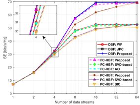
Figure 2: SE versus number of data streams ($N_{\rm r}=N_{\rm t}=64$, $\textrm{SNR}=20$ dB, and $b=3$).

V Conclusions

We have investigated precoding designs for DBF, FC-HBF, and PC-HBF architectures in massive MIMO systems with low-resolution ADCs aiming at maximizing the system SE. To solve the resulting challenging nonconvex problem, we first derive a tight lower bound for the SE and then iteratively optimize the precoder under the MM framework. Based on this method, we propose efficient precoding algorithms for DBF, FC-HBF, and PC-HBF architectures. Numerical results demonstrate that the proposed methods significantly outperform the compared benchmarks in low-resolution systems, especially with 1-bit ADCs. Furthermore, the results indicate that the PC hybrid precoding design can achieve SE comparable to those of the digital and FC hybrid precoding designs in 1-bit systems, highlighting the potential of PC-HBF architectures.