Benign or Not-Benign Overfitting
in Token Selection of Attention Mechanism
Abstract
Modern over-parameterized neural networks can be trained to fit the training data perfectly while still maintaining a high generalization performance. This “benign overfitting” phenomenon has been studied in a surge of recent theoretical work; however, most of these studies have been limited to linear models or two-layer neural networks. In this work, we analyze benign overfitting in the token selection mechanism of the attention architecture, which characterizes the success of transformer models. We first show the existence of a benign overfitting solution and explain its mechanism in the attention architecture. Next, we discuss whether the model converges to such a solution, raising the difficulties specific to the attention architecture. We then present benign overfitting cases and not-benign overfitting cases by conditioning different scenarios based on the behavior of attention probabilities during training. To the best of our knowledge, this is the first study to characterize benign overfitting for the attention mechanism.
1 Introduction
Modern over-parameterized neural networks achieve a high generalization accuracy while perfectly fitting to the training data (Zhang et al., 2021). This “benign overfitting” phenomenon has attracted attention over the past few years because it contrasts with the conventional wisdom that achieving better generalization requires balancing training error and model complexity through appropriate regularization techniques, which prevents overfitting to training noise. The theoretical understanding of benign overfitting is crucial for obtaining insights into over-parameterized networks.
There are lines of studies analyzing the benign overfitting phenomenon in various settings, linear regression (Bartlett et al., 2020; Tsigler & Bartlett, 2023), linear classification (Chatterji & Long, 2021; Cao et al., 2021), and two-layer neural networks (Frei et al., 2022; Cao et al., 2022). However, the analysis of benign overfitting is limited to these types of architecture. As far as we know, there have been no theoretical analyses on attention architecture, which is a core component of the transformer model (Vaswani et al., 2017). Given the current success of transformer models across a wide range of fields (Brown et al., 2020; Baevski et al., 2020; Dosovitskiy et al., 2021; Wei et al., 2022b, a; Touvron et al., 2023; Chowdhery et al., 2023), analyzing the attention mechanism that distinguishes them from other architectures has become increasingly significant.
The concept of benign overfitting in transformers is not yet well-defined. We do not even know what aspects should be analyzed in the first place. As a first step towards addressing this problem, we focus on analyzing token selection, a key property of the attention mechanism that characterizes transformers. We consider a one-layer attention network , where is the softmax function, is the sequence of input tokens, is a tunable token, is the key-query matrix, and is a well-pretrained linear head, on a separated binary classification task. Here, corresponds to the [CLS] token or prompt tuning in the application of transformers, and we followed the common setup studied in other topics, such as implicit bias (Tarzanagh et al., 2023a, b; Oymak et al., 2023). Our main contributions are summarized as follows:
-
•
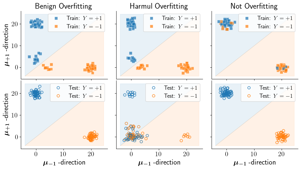
Existence of Benign Overfitting Solution (Thm 4.1): We first prove the existence of a benign overfitting solution and explain its mechanism in the token selection of attention architecture. Specifically, in addition to learning the signal with class information, benign overfitting is achieved by memorizing tokens that can fit the label noise. In this scenario, tokens that are useful for class prediction are selected for the unseen data, but for noisy data in the training set, tokens that can adapt to the noise are picked, suppressing the class-relevant tokens. This aligns with the conventional understanding of benign overfitting: the principal components explain the overall prediction, and noise memorization accounts for fitting noise. Please refer to Figure 1 for an explanation of benign overfitting in token selection, as well as other scenarios.
-
•
Convergence with Gradient Descent (Thm 4.2): We discuss whether the model weights can converge to such a benign overfitting solution with gradient descent. Two factors specific to attention models complicate the straightforward application of existing analysis: (i) the existence of local minima, which trap the optimization process, and (ii) the diminishing updates of desirable parameters as learning progresses and token selection advances. Particularly due to property (ii), the signal updates in each step are not determined based solely on the label noise ratio but rather depend on the other tokens and training data in a complex manner. In this work, we show that the one-layer attention can be trained to fit the training data with gradient descent. Then, by conditioning different scenarios of the training trajectory, we present cases where benign overfitting occurs and cases where it leads to harmful overfitting.
In this paper, we consider binary classification for simplicity of discussion, but as shown in Section F, it can be extended to the multi-class setting without fundamentally modifying the argument.
2 Related Work
Benign Overfitting.
The success of modern over-parameterized models has led to numerous studies attempting to understand why and when benign overfitting occurs. The analysis is interesting because the standard generalization bound based on uniform convergence does not explain this phenomenon well (Nagarajan & Kolter, 2019). For comprehensive surveys of the literature on this topic, please see work such as Bartlett et al. (2021); Belkin (2021).
Benign overfitting in regression has been studied in the linear model (Bartlett et al., 2020; Hastie et al., 2022) and kernel regression (Liang & Rakhlin, 2020; Tsigler & Bartlett, 2023). It is complicated to analyze the classification task because the explicit formula for the min-norm separator is not obtained. One approach is to track the training dynamics with gradient descent in the linear classifier and two-layer neural network (Chatterji & Long, 2021; Frei et al., 2022; Xu & Gu, 2023; Cao et al., 2022; Kou et al., 2023; Xu et al., 2024). Another line of work is built on the results of implicit bias to the max-margin solution (Cao et al., 2021; Wang et al., 2021; Wang & Thrampoulidis, 2022; Frei et al., 2023a). These studies base their discussion of convergence on existing research on implicit bias (Soudry et al., 2018; Ji & Telgarsky, 2019; Lyu & Li, 2020; Frei et al., 2023b). Specifically, they analyze the properties of the solution through the KKT conditions of the max-margin problem in order to examine whether the solution at convergence shows benign overfitting or not. For instance, in the setting of support vector machine, Hsu et al. (2021); Muthukumar et al. (2021) have shown that all training points become support vectors in a high-dimensional setup. The analysis becomes more challenging in the case of general deep neural networks, and Zhu et al. (2023) conducts an analysis under the neural tangent kernel (NTK) regime.
Emerging research directions have explored the benignity of overfitting, given that real-world models do not always exhibit benign overfitting. Mallinar et al. (2022) introduced the term “tempered overfitting” to analyze the overfitting between benign and catastrophic. Wen et al. (2023) examined tempered overfitting for the mild-overparameterized model, and Kornowski et al. (2024) investigated it for a two-layer ReLU neural network with low input dimensionality.
Token-selection in Attention.
The attention mechanism is a core architecture in the transformer model, and theoretical analyses from the perspectives of generalization ability (Jelassi et al., 2022; Li et al., 2023a, b) and expressive ability (Yun et al., 2020a, b; Dong et al., 2021) have been progressing in recent years. The most related line of work to ours deals with the implicit bias of gradient descent in training a one-layer attention model (Tarzanagh et al., 2023a, b; Li et al., 2024; Vasudeva et al., 2024). While these studies share common aspects with our work, their primary focus is optimizing the given training set without considering the underlying distribution (see Section 4.3 for details). Furthermore, our work is also influenced by the problem setting of (Oymak et al., 2023). However, they discuss the importance of the softmax function in the attention mechanism, whereas our work is largely different in that we focus on the fitting to label noise and benign overfitting.
3 Problem Setting
In this section, we introduce the notation and the problem settings in the rest of the paper.
3.1 Notations
We use lower-case and upper-case bold letters (e.g., and ) to represent vectors and matrices, and their entries are denoted as , . Let be a shorthand for the set . We denote a multivariate Gaussian distribution with mean vector and covariance matrix by . Denote by the softmax function. The standard Big-O notations , and are used to hide absolute constants, and we denote equality and inequality ignoring constant factors by and , respectively. Additionally, we use the symbol when its meaning is clear from the context; this denotes the possible range of values.
3.2 Attention Model
Given a sequential input , a single-head self-attention layer is
with trainable weights , and . Here, the softmax function is applied row-wise with the abuse of notation.
In practice, an additional tunable token is concatenated to the input, and this position is used for the model prediction. This setup is widely used in, for example, the classification token [CLS] in BERT (Devlin et al., 2018) and ViT (Dosovitskiy et al., 2021), and prompt-tuning technique (Li & Liang, 2021; Lester et al., 2021). Let the concatenated input be ; then the cross-attention feature between and is given by
| (1) |
where we use to denote a key-query weight matrix , and the output corresponding to the position of is denoted by . In this work, we use the model output for binary classification, leading to the output dimension being , and we denote the value prediction head by . Therefore, the model under our analysis is of the form
| (2) |
The output can be regarded as an affine combination of the token scores , using the learned softmax probabilities. We denote this token score by . Furthermore, let be a shorthand for the softmax vector .
3.3 Data Model
In the analysis of benign overfitting, we typically need to consider the specific shape of the underlying data distribution to evaluate the generalization error without using a uniform convergence argument. Data models based on signal and noise widely appear in the existing benign overfitting studies (Chatterji & Long, 2021; Frei et al., 2022; Cao et al., 2022), and ours is a natural extension to the sequential inputs of the attention model. Such data models based on signal and noise are not limited to the analysis of benign overfitting but are also commonly observed in other analyses of attention architecture (Jelassi et al., 2022; Li et al., 2023a; Oymak et al., 2023).
We consider the following data distribution defined over . In this paper, we consider binary classification for simplicity of discussion, but the same argument applies to the multi-class case. Please refer to Section F in the appendix for more details.
Definition 3.1.
Let be fixed signal vectors representing the class of each data point. The input has tokens that are split into three groups: relevant token containing the strong signal for true class, weakly relevant token containing weak class signals, and irrelevant token containing only noise. Let clean distribution be the distribution over such that is sampled as follows:
-
1.
The clean label is sampled from a uniform distribution on .
-
2.
The noise vectors are sampled independently from for some diagonal matrix . We assume the diagonal elements are positive and of constant order.
-
3.
The relevant tokens are generated with .
-
4.
The weakly relevant tokens are generated with , where is a small scale parameter, and are sampled from a uniform distribution on . For simplicity, we assume at least one token aligns with each class, which holds with high probability (see Lemma B.9 for details).
-
5.
The irrelevant tokens are generated with .
Here, we assume the ratios of relevant and weakly relevant tokens are constant and denote them by , and , respectively. The data distribution is defined as the label-corrupted version of with the level of label noise . The data point from is generated by first sampling from clean distribution and then setting with probability and with probability .
Training data are sampled i.i.d. from . We denote the clean data and noisy data by and , respectively. Furthermore, the set of data are denoted as , and are denoted as . The same notation is applied to . The superscript denotes that the variable corresponds to the training data . For instance, we write and use to represent the token scores, which were defined in the previous section. Since the input tokens to the attention model are position invariant and the token ratios are constant, we use the same notation across all samples. Although the size of is fixed, each token is randomly correlated with some class; therefore, we used the notation and for each sample to clarify the class of the weak relevance. For simplicity, we make the next assumption on the signal.
Assumption A.
The class signal vectors hold the following:
where and .
In addition, for simplicity of notation, we denote the norm of the signals by and .
Remark 1 (Weakly Relevant Token).
Weakly relevant tokens represent tokens with weak signal strength and confusing class information, reflecting a more realistic scenario than a clean separation into relevant and irrelevant tokens. For instance, if the label noise derives from annotation errors, it is plausible that weakly relevant tokens aligning with the label noise exist.
3.4 Gradient-descent Training
The learnable parameters are trained to minimize the empirical risk objective:
| (3) |
where is a binary cross-entropy loss. In this paper, since our interest lies primarily in the token-selection mechanism, i.e., the inside softmax, we will discuss benign overfitting of under a fixed well-pretrained linear head . This setup is supported by the following facts.
Lemma 3.1 (Informal).
Suppose that . Then, the gradient descent direction of the empirical risk at aligns with .
In the general multi-class case, the gradient direction of the expected risk aligns with the Equiangular Tight Frame (ETF) with class vectors (Papyan et al., 2020), which will be discussed in Section G in the appendix. The final layer fixed to ETF geometry during the training is often observed in the context of imbalanced data and transfer learning (Yang et al., 2022; Ali et al., 2024).
The remaining trainable parameters are ; however, they essentially play the same role inside the softmax function, as shown in Lemma A.6. Thus, we only consider optimizing inside softmax and fixing throughout training. Let be initialized as follows and fixed in the rest of the paper.
Assumption B.
The weight is initialized with the orthogonal matrix: .
Let be initialized as ; therefore, for any input, the model calculates the uniform attention at time step . The parameters are optimized by gradient descent with a step size :
| (4) |
Let and be the and after the gradient descent step, respectively. We also denote the Lipschitz constant of by , which represents the smoothness of the empirical loss function.
3.5 Assumption on Parameters
In this section, we first discuss the necessity of the assumptions on parameters and compare them with existing studies, followed by a list of the assumptions used in our work. In analyzing benign overfitting, the balance between memorization and generalization is significant. Therefore, we impose assumptions on the balance between the dimensionality and the signal strength .
The over-parameterization assumptions (A1) and (A’1) are necessary for fitting label noise, and similar terms can be found in (Chatterji & Long, 2021; Frei et al., 2022; Kou et al., 2023). Assumptions (A2) and (A’2) are required for generalization, while in the right-hand side also appears in (Xu & Gu, 2023), and is found in (Xu et al., 2024). For these assumptions on and , since this is the first analysis of benign overfitting in the attention architecture, the dependence on sequence length is newly introduced, and the difficulties unique to this setting, which will be discussed later in Section 4.3, involve stronger assumptions. Assumptions (A3) and (A’3) are also necessary for fitting label noise, and (A’3) is stronger for simplifying the conditions in Theorem 4.2. This assumption is non-vacuous because the value of can take in a wide range when and are significantly larger than and . For example, is assumed in (Cao et al., 2022), which is based on a similar proof technique to ours. Assumptions (A5) and (A6) are placed to evaluate the class balance in the training data and the amount of noisy data, but in this paper, they are absorbed into the conditions of Eqs.9-13 and are not directly used.
Now, we state our assumptions in the following. Given a small failure probability and a large enough universal constant , we make the assumptions for each parameter as follows:
-
(A1)
The covariance matrix satisfies .
-
(A2)
The signal strength satisfies .
-
(A3)
The weak signal strength satisfies .
-
(A4)
The step size satisfies .
-
(A5)
The number of training data satisfies .
-
(A6)
The noise rate satisfies .
Furthermore, stronger versions of assumption (A1), (A2), (A3) are introduced to discuss the convergence of the gradient descent in Theorem 4.2.
-
(A’1)
The covariance matrix satisfies .
-
(A’2)
The signal strength satisfies .
-
(A’3)
The weak signal satisfies .
In addition, the equations derived from these assumptions, which will be used in our proofs, are presented in Lemma A.8 in the appendix.
4 Main Results
In this section, we first demonstrate the existence of a benign overfitting solution in Section 4.1 and then discuss the convergence of gradient descent towards this benign overfitting solution in Section 4.2. Finally, in Section 4.3, we explain the unique difficulties posed by the attention architectures in analyzing benign overfitting and provide justification for the conditions used in the theorem and approach adopted in this work.
4.1 Existence of Benign Overfitting
We first show the existence of the solution that exhibits benign overfitting. This result is useful for explaining the key idea that both signal learning and noise memorization are necessary for benign overfitting in token selection. Here, note that the model simply learning the signal vectors does not overfit to noisy data.
Theorem 4.1 (Existence of benign overfitting solution).
Suppose that the assumptions (A1)-(A6) hold. Let the linear head be fixed during the training, and be some constants. For any weakly relevant token , which aligns with label noise and sufficiently large constant ,
is a benign overfitting solution with probability at least . In other words, we have
-
1.
(Overfitting) The model overfits to the training data with label noise:
(5) -
2.
(Generalization) The generalization loss of is bounded as:
(6)
4.2 Convergence to Benign Overfitting
While we have seen the existence of a benign overfitting solution, we will further analyze in this section whether gradient descent converges to such a solution and what conditions are necessary for benign overfitting. Theorem 4.1 shows that both the signal required for generalization and the noise memorization for fitting label noise are significant, and their balance is essential for benign overfitting. In practice, the model is trained by gradient descent based on the empirical loss function; therefore, we must handle the influence of label noise in the signal learning, and noise memorization occurs for all tokens besides the desirable token , making it challenging to draw simple conclusions for optimization.
Before presenting the statement, we introduce the following value, which is crucial for understanding the gradient descent behavior in the attention architecture.
Definition 4.1 (Uncertainty in probability of picking relevant token).
For any and time step , we define as:
| (7) |
where recall that be a shorthand for the softmax probability .
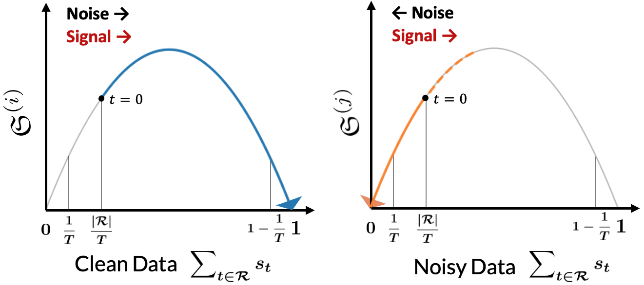
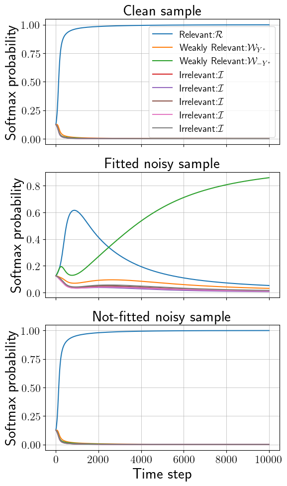
This value can be interpreted as the variance of the Bernoulli distribution, where the parameter is the attention probability assigned to the relevant token of training sample at time step . This behavior is crucial in the analysis of signal learning. Specifically, in learning signal vectors, the balance between the contributions of from clean data and from noisy data is significant and determines the progress of signal learning at time step . Figure 2 illustrates the training dynamics of this quantity for clean and noisy data. As shown later, the softmax probability converges to either or for any token under the parameter assumptions. Therefore, will eventually converge to as illustrated in Figure 2.
By dividing cases for the behavior of , we obtain the following results for the convergence.
Theorem 4.2 (Convergence of benign overfitting solution).
Suppose that the assumptions (A’1)-(A’3), (A4)-(A6) hold, and the norm of the fixed linear head scales as . With probability of at least , there exists a sufficiently large time step , and for all time step after it: , the model overfits to the training data with label noise:
| (8) |
At this time, we can further discuss the generalization error of the model if the following conditions on the training trajectory are satisfied:
-
1.
For any class, the time accumulation of summed up in the clean data dominates the accumulation of each :
(9) -
2.
The time accumulation of summed up in the clean data is balanced among labels:
(10)
Here are some absolute constants. Then, we have
-
1.
(Benign) For any class , if the training trajectory satisfies
(11) for some constant , then with probability at least , the weight is a benign overfitting solution:
(12) -
2.
(Harmful) For any class , if the training trajectory satisfies
(13) for some constant , then the weight is a not-benign overfitting solution:
(14)
This theorem shows that under the assumptions in Section 3.5, the model overfits the training data with gradient descent, and it further reduces the discussion of generalization ability to the accumulation of during the training. The reason for requiring such conditions on will be discussed later in Section 4.3. The condition Eq.9 requires that the total sum of the cumulative over the clean data exceeds the accumulation of for each data point. The condition Eq.10 concerns the balance of the cumulative among classes, and in the existing analysis not involving softmax probability, it is straightforward to verify that the number of samples for each class in the training data is equal ignoring constants with high probability.
4.3 Difficulty Specific to Attention Analysis
In this section, we compare our work with the existing analysis of benign overfitting (Chatterji & Long, 2021; Frei et al., 2022; Xu & Gu, 2023) tracking gradient descent dynamics, which is the approach we took in this work, and highlight the unique difficulties inherent in the attention architecture. The first two paragraphs focus on these difficulties, and in the final part, we explain the limitations of the other approach.
Presence of local minima.
The first difficulty comes from the presence of local minima that do not fit all the training data. In the previous settings, the gradient of the loss function (or the margin increase) at each time step can be bounded below by some form of training error; therefore, proving convergence of the gradient implies overfitting to the training set. In this paper setting, the gradient of the empirical loss function is given as follows:
| (15) |
where is the derivative of the binary cross-entropy loss, given in Eq.3. Since the learning token selection does not change the scale of output, the term does not converge to zero, and the gradient becomes zero only when the attention probabilities converge to or , as will be shown in Lemma D.3. Therefore, undesirable tokens can be picked even when the gradient becomes zero, and we have to track the dynamics of token probability during training.
Diminishing parameter updates due to softmax.
The second difficulty is that the gradient descent updates are involved with the softmax probabilities. The relationship between the contributions from clean and noisy data, as well as the updates for signals and noises, cannot be evaluated independently of the current time step, as the gradient descent updates depend on the value of . As shown in Figure 2, the closer the probability of selecting the desired token approaches , the smaller the updates will be for selecting that token. This diminishing growth of model parameters complicates the convergence analysis of benign overfitting in the attention, compared to existing work on linear classifiers and two-layer networks. For example, while relevant tokens in the clean data are quickly picked, driving toward , if is still large in noisy data (i.e., not yet near both ends in Figure 2), the contribution of noisy data to the learning can become more significant than that of clean data even when the number of noisy data is much smaller.
Obstacles in approach from max-margin problem
One potential approach is based on the convergence of max-margin solutions for token-separation (Tarzanagh et al., 2023b; Vasudeva et al., 2024), similar to the existing work using KKT conditions. However, this approach is challenging for two reasons: 1) there is no guarantee of global convergence of the max-margin problem, and 2) there is a mismatch between the max-margin solution and the local solution of empirical loss due to the difference in token scores. Please refer to Section H in the appendix for further details.
5 Experiments
In this section, we conduct synthetic experiments based on the data model in Definition 3.1 to support our analysis. The code used for the experiments is available on GitHub 111https://github.com/keitaroskmt/benign-attention.
Synthetic Experiments.
We train the same model as in Eq.2 with gradient descent, using the same data model as Definition 3.1 with the covariance matrix . Specifically, we consider the setting with , , , and , changing the value of the dimension and the signal size . For simplicity, we set and .
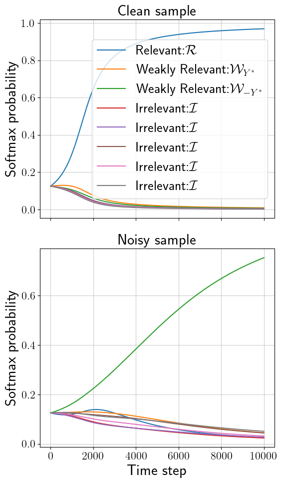
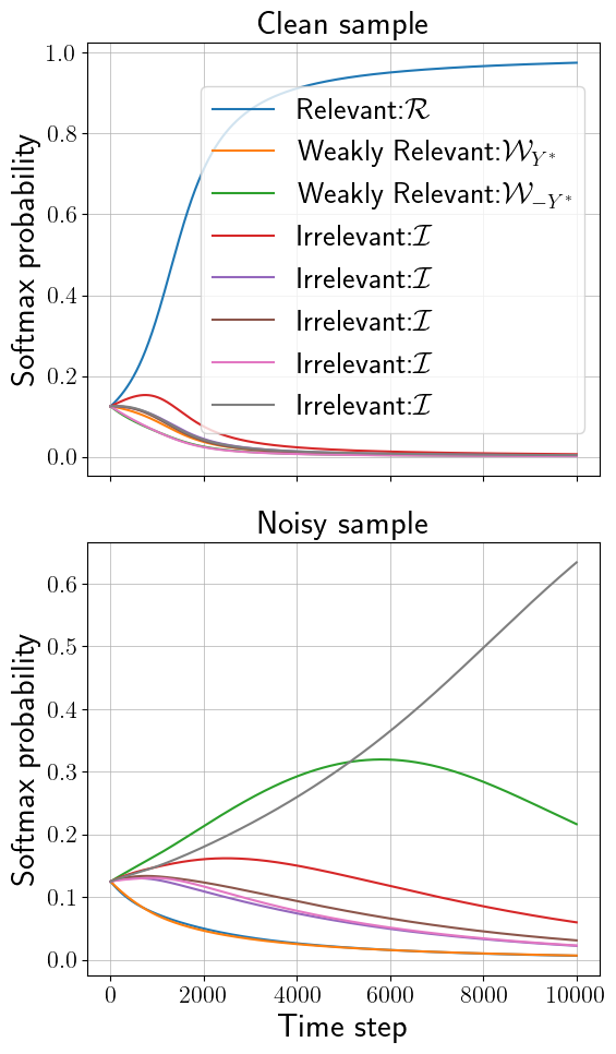
Figure 3 shows the dynamics of softmax probabilities for clean and noisy training samples from the initial value . The left figure shows the case where benign overfitting is achieved, and selecting the weakly relevant token for the noisy data aligns with our analysis. In the middle, where the is larger compared to , memorization becomes dominant. The bottom figure shows that weakly relevant tokens are not always selected for noisy data; instead, irrelevant tokens that fit the label noise are picked. This model can fit the training data with noise components, which hinders signal learning and reduces generalization ability. In the right figure, where signal norm is large, fitting the noisy data becomes challenging. The middle of Figure 3(c) shows that the model successfully selects weakly relevant tokens aligning with the label noise, but in the bottom figure, some noisy data are influenced toward selecting relevant tokens that should not be chosen for fitting noisy data. Finally, the heat maps for train and test loss when varying the dimension and the signal norm are shown in Figure 6 in the appendix. We can see that the balance between the dimension and the signal norm is significant for achieving low train and test loss.
Validity of Conditions in Theorem 4.2.
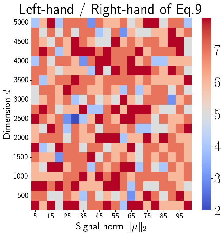
Furthermore, we verify the conditions in Theorem 4.2. Figure 4 shows the ratio of the left-hand side to the right-hand side of Eq. 9 when varying and . The key point here is that the ratio exceeds in all settings and training runs. The current setup is and , with a small number of clean data in the same class, but the condition Eq.9 is expected to hold more easily when is larger. As for the class balance condition in Eq.10, the results are provided in Section I in the appendix due to space limitation.
6 Conclusion
In this paper, we analyzed benign overfitting in the token selection of the attention architecture and further supported the analysis with synthetic experiments. As a natural next step, a more detailed technical analysis of the attention probability behavior during training, which appeared as conditions in our results, can be considered. Additionally, extending the attention analysis to next-token prediction or a full self-attention model is also an interesting research direction.
References
- Ali et al. (2024) Hafiz Tiomoko Ali, Umberto Michieli, Ji Joong Moon, Daehyun Kim, and Mete Ozay. Deep neural network models trained with a fixed random classifier transfer better across domains. In ICASSP 2024-2024 IEEE International Conference on Acoustics, Speech and Signal Processing (ICASSP), pp. 5305–5309. IEEE, 2024.
- Baevski et al. (2020) Alexei Baevski, Yuhao Zhou, Abdelrahman Mohamed, and Michael Auli. wav2vec 2.0: A framework for self-supervised learning of speech representations. Advances in neural information processing systems, 33:12449–12460, 2020.
- Bartlett et al. (2020) Peter L Bartlett, Philip M Long, Gábor Lugosi, and Alexander Tsigler. Benign overfitting in linear regression. Proceedings of the National Academy of Sciences, 117(48):30063–30070, 2020.
- Bartlett et al. (2021) Peter L Bartlett, Andrea Montanari, and Alexander Rakhlin. Deep learning: a statistical viewpoint. Acta numerica, 30:87–201, 2021.
- Belkin (2021) Mikhail Belkin. Fit without fear: remarkable mathematical phenomena of deep learning through the prism of interpolation. Acta Numerica, 30:203–248, 2021.
- Boucheron et al. (2003) Stéphane Boucheron, Gábor Lugosi, and Olivier Bousquet. Concentration inequalities. In Summer school on machine learning, pp. 208–240. Springer, 2003.
- Brown et al. (2020) Tom Brown, Benjamin Mann, Nick Ryder, Melanie Subbiah, Jared D Kaplan, Prafulla Dhariwal, Arvind Neelakantan, Pranav Shyam, Girish Sastry, Amanda Askell, et al. Language models are few-shot learners. Advances in neural information processing systems, 33:1877–1901, 2020.
- Cao et al. (2021) Yuan Cao, Quanquan Gu, and Mikhail Belkin. Risk bounds for over-parameterized maximum margin classification on sub-gaussian mixtures. Advances in Neural Information Processing Systems, 34:8407–8418, 2021.
- Cao et al. (2022) Yuan Cao, Zixiang Chen, Misha Belkin, and Quanquan Gu. Benign overfitting in two-layer convolutional neural networks. Advances in neural information processing systems, 35:25237–25250, 2022.
- Chatterji & Long (2021) Niladri S Chatterji and Philip M Long. Finite-sample analysis of interpolating linear classifiers in the overparameterized regime. Journal of Machine Learning Research, 22(129):1–30, 2021.
- Chowdhery et al. (2023) Aakanksha Chowdhery, Sharan Narang, Jacob Devlin, Maarten Bosma, Gaurav Mishra, Adam Roberts, Paul Barham, Hyung Won Chung, Charles Sutton, Sebastian Gehrmann, et al. Palm: Scaling language modeling with pathways. Journal of Machine Learning Research, 24(240):1–113, 2023.
- Devlin et al. (2018) Jacob Devlin, Ming-Wei Chang, Kenton Lee, and Kristina Toutanova. Bert: Pre-training of deep bidirectional transformers for language understanding. arXiv preprint arXiv:1810.04805, 2018.
- Dong et al. (2021) Yihe Dong, Jean-Baptiste Cordonnier, and Andreas Loukas. Attention is not all you need: pure attention loses rank doubly exponentially with depth. In Marina Meila and Tong Zhang (eds.), Proceedings of the 38th International Conference on Machine Learning, volume 139 of Proceedings of Machine Learning Research, pp. 2793–2803. PMLR, 18–24 Jul 2021. URL https://proceedings.mlr.press/v139/dong21a.html.
- Dosovitskiy et al. (2021) Alexey Dosovitskiy, Lucas Beyer, Alexander Kolesnikov, Dirk Weissenborn, Xiaohua Zhai, Thomas Unterthiner, Mostafa Dehghani, Matthias Minderer, Georg Heigold, Sylvain Gelly, Jakob Uszkoreit, and Neil Houlsby. An image is worth 16x16 words: Transformers for image recognition at scale. In International Conference on Learning Representations, 2021. URL https://openreview.net/forum?id=YicbFdNTTy.
- Frei et al. (2022) Spencer Frei, Niladri S Chatterji, and Peter Bartlett. Benign overfitting without linearity: Neural network classifiers trained by gradient descent for noisy linear data. In Conference on Learning Theory, pp. 2668–2703. PMLR, 2022.
- Frei et al. (2023a) Spencer Frei, Gal Vardi, Peter Bartlett, and Nathan Srebro. Benign overfitting in linear classifiers and leaky relu networks from kkt conditions for margin maximization. In The Thirty Sixth Annual Conference on Learning Theory, pp. 3173–3228. PMLR, 2023a.
- Frei et al. (2023b) Spencer Frei, Gal Vardi, Peter Bartlett, Nathan Srebro, and Wei Hu. Implicit bias in leaky reLU networks trained on high-dimensional data. In The Eleventh International Conference on Learning Representations, 2023b. URL https://openreview.net/forum?id=JpbLyEI5EwW.
- Hastie et al. (2022) Trevor Hastie, Andrea Montanari, Saharon Rosset, and Ryan J Tibshirani. Surprises in high-dimensional ridgeless least squares interpolation. Annals of statistics, 50(2):949, 2022.
- Hsu et al. (2021) Daniel Hsu, Vidya Muthukumar, and Ji Xu. On the proliferation of support vectors in high dimensions. In International Conference on Artificial Intelligence and Statistics, pp. 91–99. PMLR, 2021.
- Jelassi et al. (2022) Samy Jelassi, Michael Sander, and Yuanzhi Li. Vision transformers provably learn spatial structure. Advances in Neural Information Processing Systems, 35:37822–37836, 2022.
- Ji & Telgarsky (2019) Ziwei Ji and Matus Telgarsky. The implicit bias of gradient descent on nonseparable data. In Alina Beygelzimer and Daniel Hsu (eds.), Proceedings of the Thirty-Second Conference on Learning Theory, volume 99 of Proceedings of Machine Learning Research, pp. 1772–1798. PMLR, 25–28 Jun 2019. URL https://proceedings.mlr.press/v99/ji19a.html.
- Kornowski et al. (2024) Guy Kornowski, Gilad Yehudai, and Ohad Shamir. From tempered to benign overfitting in relu neural networks. Advances in Neural Information Processing Systems, 36, 2024.
- Kou et al. (2023) Yiwen Kou, Zixiang Chen, Yuanzhou Chen, and Quanquan Gu. Benign overfitting in two-layer relu convolutional neural networks. In International Conference on Machine Learning, pp. 17615–17659. PMLR, 2023.
- Lester et al. (2021) Brian Lester, Rami Al-Rfou, and Noah Constant. The power of scale for parameter-efficient prompt tuning. arXiv preprint arXiv:2104.08691, 2021.
- Li et al. (2023a) Hongkang Li, Meng Wang, Sijia Liu, and Pin-Yu Chen. A theoretical understanding of shallow vision transformers: Learning, generalization, and sample complexity. In The Eleventh International Conference on Learning Representations, 2023a. URL https://openreview.net/forum?id=jClGv3Qjhb.
- Li & Liang (2021) Xiang Lisa Li and Percy Liang. Prefix-tuning: Optimizing continuous prompts for generation. arXiv preprint arXiv:2101.00190, 2021.
- Li et al. (2023b) Yingcong Li, Muhammed Emrullah Ildiz, Dimitris Papailiopoulos, and Samet Oymak. Transformers as algorithms: Generalization and stability in in-context learning. In International Conference on Machine Learning, pp. 19565–19594. PMLR, 2023b.
- Li et al. (2024) Yingcong Li, Yixiao Huang, Muhammed E Ildiz, Ankit Singh Rawat, and Samet Oymak. Mechanics of next token prediction with self-attention. In International Conference on Artificial Intelligence and Statistics, pp. 685–693. PMLR, 2024.
- Liang & Rakhlin (2020) Tengyuan Liang and ALexander Rakhlin. Just interpolate: Kernel “ridgeless” regression can generalize. The Annals of Statistics, 48(3):1329–1347, 2020.
- Lyu & Li (2020) Kaifeng Lyu and Jian Li. Gradient descent maximizes the margin of homogeneous neural networks. In International Conference on Learning Representations, 2020. URL https://openreview.net/forum?id=SJeLIgBKPS.
- Mallinar et al. (2022) Neil Mallinar, James Simon, Amirhesam Abedsoltan, Parthe Pandit, Misha Belkin, and Preetum Nakkiran. Benign, tempered, or catastrophic: Toward a refined taxonomy of overfitting. Advances in Neural Information Processing Systems, 35:1182–1195, 2022.
- Muthukumar et al. (2021) Vidya Muthukumar, Adhyyan Narang, Vignesh Subramanian, Mikhail Belkin, Daniel Hsu, and Anant Sahai. Classification vs regression in overparameterized regimes: Does the loss function matter? Journal of Machine Learning Research, 22(222):1–69, 2021.
- Nagarajan & Kolter (2019) Vaishnavh Nagarajan and J Zico Kolter. Uniform convergence may be unable to explain generalization in deep learning. Advances in Neural Information Processing Systems, 32, 2019.
- Oymak et al. (2023) Samet Oymak, Ankit Singh Rawat, Mahdi Soltanolkotabi, and Christos Thrampoulidis. On the role of attention in prompt-tuning. In International Conference on Machine Learning, pp. 26724–26768. PMLR, 2023.
- Papyan et al. (2020) Vardan Papyan, XY Han, and David L Donoho. Prevalence of neural collapse during the terminal phase of deep learning training. Proceedings of the National Academy of Sciences, 117(40):24652–24663, 2020.
- Soudry et al. (2018) Daniel Soudry, Elad Hoffer, Mor Shpigel Nacson, Suriya Gunasekar, and Nathan Srebro. The implicit bias of gradient descent on separable data. Journal of Machine Learning Research, 19(70):1–57, 2018.
- Tarzanagh et al. (2023a) Davoud Ataee Tarzanagh, Yingcong Li, Christos Thrampoulidis, and Samet Oymak. Transformers as support vector machines. arXiv preprint arXiv:2308.16898, 2023a.
- Tarzanagh et al. (2023b) Davoud Ataee Tarzanagh, Yingcong Li, Xuechen Zhang, and Samet Oymak. Max-margin token selection in attention mechanism. In Thirty-seventh Conference on Neural Information Processing Systems, 2023b. URL https://openreview.net/forum?id=WXc8O8ghLH.
- Touvron et al. (2023) Hugo Touvron, Thibaut Lavril, Gautier Izacard, Xavier Martinet, Marie-Anne Lachaux, Timothée Lacroix, Baptiste Rozière, Naman Goyal, Eric Hambro, Faisal Azhar, et al. Llama: Open and efficient foundation language models. arXiv preprint arXiv:2302.13971, 2023.
- Tsigler & Bartlett (2023) Alexander Tsigler and Peter L Bartlett. Benign overfitting in ridge regression. Journal of Machine Learning Research, 24(123):1–76, 2023.
- Vasudeva et al. (2024) Bhavya Vasudeva, Puneesh Deora, and Christos Thrampoulidis. Implicit bias and fast convergence rates for self-attention. arXiv preprint arXiv:2402.05738, 2024.
- Vaswani et al. (2017) Ashish Vaswani, Noam Shazeer, Niki Parmar, Jakob Uszkoreit, Llion Jones, Aidan N Gomez, Łukasz Kaiser, and Illia Polosukhin. Attention is all you need. Advances in neural information processing systems, 30, 2017.
- Vershynin (2018) Roman Vershynin. High-dimensional probability: An introduction with applications in data science, volume 47. Cambridge university press, 2018.
- Wainwright (2019) Martin J. Wainwright. High-Dimensional Statistics: A Non-Asymptotic Viewpoint. Cambridge Series in Statistical and Probabilistic Mathematics. Cambridge University Press, 2019.
- Wang & Thrampoulidis (2022) Ke Wang and Christos Thrampoulidis. Binary classification of gaussian mixtures: Abundance of support vectors, benign overfitting, and regularization. SIAM Journal on Mathematics of Data Science, 4(1):260–284, 2022.
- Wang et al. (2021) Ke Wang, Vidya Muthukumar, and Christos Thrampoulidis. Benign overfitting in multiclass classification: All roads lead to interpolation. Advances in Neural Information Processing Systems, 34:24164–24179, 2021.
- Wei et al. (2022a) Jason Wei, Yi Tay, Rishi Bommasani, Colin Raffel, Barret Zoph, Sebastian Borgeaud, Dani Yogatama, Maarten Bosma, Denny Zhou, Donald Metzler, Ed H. Chi, Tatsunori Hashimoto, Oriol Vinyals, Percy Liang, Jeff Dean, and William Fedus. Emergent abilities of large language models. Transactions on Machine Learning Research, 2022a. ISSN 2835-8856. URL https://openreview.net/forum?id=yzkSU5zdwD. Survey Certification.
- Wei et al. (2022b) Jason Wei, Xuezhi Wang, Dale Schuurmans, Maarten Bosma, Fei Xia, Ed Chi, Quoc V Le, Denny Zhou, et al. Chain-of-thought prompting elicits reasoning in large language models. Advances in neural information processing systems, 35:24824–24837, 2022b.
- Wen et al. (2023) Kaiyue Wen, Jiaye Teng, and Jingzhao Zhang. Benign overfitting in classification: Provably counter label noise with larger models. In The Eleventh International Conference on Learning Representations, 2023. URL https://openreview.net/forum?id=UrEwJebCxk.
- Xu & Gu (2023) Xingyu Xu and Yuantao Gu. Benign overfitting of non-smooth neural networks beyond lazy training. In International Conference on Artificial Intelligence and Statistics, pp. 11094–11117. PMLR, 2023.
- Xu et al. (2024) Zhiwei Xu, Yutong Wang, Spencer Frei, Gal Vardi, and Wei Hu. Benign overfitting and grokking in reLU networks for XOR cluster data. In The Twelfth International Conference on Learning Representations, 2024. URL https://openreview.net/forum?id=BxHgpC6FNv.
- Yang et al. (2022) Yibo Yang, Shixiang Chen, Xiangtai Li, Liang Xie, Zhouchen Lin, and Dacheng Tao. Inducing neural collapse in imbalanced learning: Do we really need a learnable classifier at the end of deep neural network? Advances in neural information processing systems, 35:37991–38002, 2022.
- Yun et al. (2020a) Chulhee Yun, Srinadh Bhojanapalli, Ankit Singh Rawat, Sashank Reddi, and Sanjiv Kumar. Are transformers universal approximators of sequence-to-sequence functions? In International Conference on Learning Representations, 2020a. URL https://openreview.net/forum?id=ByxRM0Ntvr.
- Yun et al. (2020b) Chulhee Yun, Yin-Wen Chang, Srinadh Bhojanapalli, Ankit Singh Rawat, Sashank Reddi, and Sanjiv Kumar. O (n) connections are expressive enough: Universal approximability of sparse transformers. Advances in Neural Information Processing Systems, 33:13783–13794, 2020b.
- Zhang et al. (2021) Chiyuan Zhang, Samy Bengio, Moritz Hardt, Benjamin Recht, and Oriol Vinyals. Understanding deep learning (still) requires rethinking generalization. Communications of the ACM, 64(3):107–115, 2021.
- Zhu et al. (2023) Zhenyu Zhu, Fanghui Liu, Grigorios Chrysos, Francesco Locatello, and Volkan Cevher. Benign overfitting in deep neural networks under lazy training. In International Conference on Machine Learning, pp. 43105–43128. PMLR, 2023.
Appendix A Preliminaries
A.1 Notation
We first list the notations used in this work in Table 1.
| Sequence of input tokens, | |
| Noise corrupted label | |
| True label | |
| Length of input tokens | |
| Dimension of token embedding | |
| Number of training data | |
| Probability vector for at -th step, | |
| Token score, | |
| Signal vectors for class and , respectively | |
| Coefficients for and , respectively, in the parameter | |
| Covariance matrix of noise vector | |
| Noise component in | |
| Coefficient for in the parameter | |
| Set of relevant token: | |
| Set of weakly relevant token: | |
| Set of weak relevant token with specific label, , . We also use the notation and for the input . | |
| Set of irrelevant token: | |
| Ratio of relevant and weakly relevant tokens: , | |
| Value defined as | |
| Set of clean data: | |
| Set of clean data with label and , respectively | |
| Set of noisy data: | |
| Set of noisy data with label and , respectively | |
| Learning rate | |
| Level of label noise | |
| Index used mainly for or | |
| Index used mainly for | |
| Index used mainly for | |
| Index used mainly for or | |
| Index used mainly for |
Furthermore, the basic computations are presented here for convenience.
The gradient used in the training can be explicitly computed as follows. Since the derivative of the softmax function is given by
where denotes the diagonal matrix whose -th entry equals to . Using the denominator layout, we have
| (16) | ||||
| (17) | ||||
| (18) |
where is abbreviation for .
A.2 Proof Sketch
In this section, we briefly introduce the proof sketch of the main theorem along with the key lemmas to provide the road maps in the appendix. The whole proof of Theorem 4.1 is provided in Section C, and the proof of Theorem 4.2 is completed in Section E. We first show that the following events occur simultaneously with high probability under the assumptions in Section 3.5.
Lemma A.1.
Suppose that the assumptions (A1)-(A6) hold. There exists some constant and , which depends on , such that for all , the following hold simultaneously with probability at least over the realization of training data :
-
(i)
(Noise Norm) For all , we have
(19) -
(ii)
(Noise Inner-product) For any such that , we have
(20) -
(iii)
(Signal-Noise Inner-product) For all , we have
(21) -
(iv)
Regarding the true label and the label noise, we have
(22) (23)
In the proof of the main theorems, we discuss the properties that occur with high probability by conditioning on these events. Lemma A.1 implies that a good run occurs with the probability at least over the realization of training data . The proof of Lemma A.1 will be provided in Section B. The proof of Theorem 4.1 is based on these concentration inequalities and detailed evaluations of the softmax probabilities. For the complete proof, please refer to Section C.
The convergence analysis, due to the difficulties stated in Section 4.3, follows an approach of tracking the dynamics of the signal and noise components in the gradient method rather than setting desired converged weights and evaluating the alignment with them. Specifically, let be a gradient iteration at -th time step; then, there exists unique coefficients such that
| (24) |
We will provide the complete form of this statement in Lemma D.1 and also refer to the recurrence equations that the coefficients should satisfy. Our discussion for the convergence is based on the following lemma, which leverages the smoothness of the one-layer attention network:
Lemma A.2.
Suppose the step size satisfies the assumption (A4). Then, there exists the token index for each , and we have
| (25) |
for all .
We will further confirm that the desired token is picked at the converted weights. The following two lemmas describe the relationship among the attention probabilities that hold at any time step for both clean and noisy data.
Lemma A.3.
Lemma A.4.
Using these lemmas, we can demonstrate overfitting in Theorem 4.2. Please refer to Section E.1 for the complete proof.
Next, we will discuss the generalization ability of this overfitted solution, which is closely related to the sign and order of the coefficients of the learned signal components, i.e., in Eq.24. The following is a critical lemma that shows how the conditions in the statement of Theorem 4.2 affect in the decomposition given by Eq.24.
Lemma A.5 (Simplified Version).
This lemma states that the signal coefficients are balanced among the classes in terms of order and that the learning process is not primarily a memorization of noise. If Eq.13 holds, we have a similar result where the signal coefficient becomes negative. For its proof and impact on the generalization ability, please refer to Section E as a complete proof of generalization part of Theorem 4.2.
A.3 Preliminary Lemmas
Firstly, we introduce the lemmas necessary in preparation for the main proof.
The following lemma indicates that the dynamics of can be described by the dynamics of . It justifies optimizing alone while keeping fixed throughout training. This is also intuitively understood from the fact that the gradient update of always results in a rank-1 matrix. Since some modifications have been made to the original form, we will provide the statement with proof.
Lemma A.6 (Rephrased from (Tarzanagh et al. (2023b), Lemma 1)).
Fix the linear head throughout training. On the same training data , we define
where and are fixed vector and matrix, respectively. Here, we assume that is an orthogonal matrix, following assumption B. Consider the gradient descent iterations on and with initial values and and step sizes and , respectively:
Then, we have that for all .
Proof.
We will proceed with induction. At time step , the claim holds from the definition of and . Suppose that the claim at time step holds. Since we have,
| (29) | ||||
| (30) |
we obtain using the induction hypothesis and the fact that is an orthogonal matrix. Therefore, we have
| (31) | ||||
| (32) | ||||
| (33) | ||||
| (34) |
which concludes the proof. ∎
Next, we will give the smoothness of the objective function with respect to , and as a property derived from this, we will show that the gradient will converge to zero with a sufficiently small step size. This is essentially a restatement of Lemma 6 in (Tarzanagh et al., 2023b), so please refer to that for the proof. We used assumption B and explicitly expressed as the binary cross-entropy loss.
Lemma A.7 (Rephrased from (Tarzanagh et al. (2023b), Lemma 6)).
The function is L-smooth, where
| (35) |
Furthermore, if a step size satisfies , then, for any initialization , we have
| (36) |
for all . This implies that
| (37) |
Remark 2 (Smoothness under our data model).
Lemma A.7 provides the smoothness of the empirical loss function using the operator norm of the training data inputs. Assumption (A4) requires that the step size is less than , and we comment on how small this value can be in the worst case under our data model. Here, suppose that the scale of the linear head is , and under Definition 3.1 for the data model, on a good run, we have
| (39) |
for any . Since , the smoothness in Lemma A.7 is upper-bounded as:
| (40) | ||||
| (41) | ||||
| (42) | ||||
| (43) |
where the first inequality follows from Lemma A.7 and the next is derived by Eq.39. We use the inequality and in the third inequality, and the last line follows from the assumption (A2), which implies . Consequently, we can bound the smoothness in Lemma A.7 by .
Finally, we derive the equations that can be deduced from the assumptions in Section 3.5 and will be used in the remainder of the proof.
Lemma A.8.
Proof.
We will derive the equations using the assumptions. Combining assumption (A1) and (A2) gives us:
| (47) |
By rearranging this, we obtain Eq.44. From assumption (A’3), we have
| (48) | ||||
| (49) |
where the last line follows from assumption (A’1), and Eq.45 is derived. Finally, by combining assumptions (A’1) and (A’2), we have
| (50) |
therefore, Eq.46 is shown by rearranging this equation. ∎
Appendix B Proof of Lemma A.1
In this section, we will prove each high-probability event described in Lemma A.1. Specifically, we can show it by combining Lemma B.3, B.5, B.6, and B.8, using union bound argument. In the rest of this section, suppose that assumptions (A1)-(A6) hold.
First, we show the norm concentration of the Gaussian noise vectors. The next lemma gives the lower bound for the expectation of the norm.
Lemma B.1.
For a Gaussian vector , we have
| (51) |
Proof of Lemma B.1.
We use the Gaussian Poincaré Inequality (Boucheron et al. (2003), Theorem 3.20):
| (52) |
where is any continuously differentiable function. By taking as , since we have ,
| (53) |
Rearranging the terms, we get
| (54) |
which concludes the proof. ∎
The following lemma is about the concentration of Lipschitz functions and is used to prove the norm concentration.
Lemma B.2 (Rephrased from (Wainwright (2019), Theorem 3.16)).
For any -Lipschitz function , we have
| (55) |
Note that the coefficient could be removed in the case of one-sided inequality.
Remark 3.
Generally, this holds for strongly log-concave distributions, i.e., distributions with a density , where is a strongly convex function. Here, we used the fact that the Gaussian distribution is a strongly log-concave distribution with parameter .
We are now ready to prove the norm concentration as follows.
Lemma B.3 (Norm concentration).
There exists some constant depending on such that with probability at least ,
| (56) |
for all
Proof of Lemma B.3.
From the definition of noise distribution, for all . To begin with, we show the norm concentration of the Gaussian vector. For , since we have
| (57) |
is -Lipschitz function. Using Lemma B.2, we get
| (58) |
for some . Taking union-bound gives
| (59) |
Lemma B.1 and Jensen inequality lead the following bound on the expectation of the Gaussian norm:
| (60) |
Next, we move on to the concentration inequality for the Gaussian random variables.
Lemma B.4 (Gaussian tail bound, (Vershynin (2018), Prop 2.1.2)).
For a Gaussian variable , the tail bound is given by
| (64) |
Using this, we can show the following result for the inner products of the noise vectors.
Lemma B.5 (Inner-product of Noises).
There exists some constant such that with the probability at least ,
| (65) |
for all .
Proof of Lemma B.5.
Before delving into the main part of the proof, we first show
| (66) |
for the Gaussian vector . This is a result of the concentration inequality for the norm of Gaussian distribution, but unlike Lemma B.3, it handles the norm itself rather than the deviation around the mean of the norm, which is more useful to prove this lemma.
Let , then follows the same distribution as . Since for , for any ,
| (67) | ||||
| (68) | ||||
| (69) | ||||
| (70) | ||||
| (71) |
where the second inequality follows from Markov inequality and the last follows from the moment-generating function of Gaussian distribution. Minimizing the upper bound over gives the desired inequality Eq. 66.
Fix and . For any , we have
| (72) |
where we used the inequality for the event , which gives tighter bound when outlier event and event share large common parts.
Under the condition is fixed, since follows , Lemma B.4 gives
| (73) |
Thus, the conditional probability is bounded
| (74) |
Combining Eqs. 66 and 74 then applying union bound on 72, we obtain
| (75) | ||||
| (76) |
Let for some constant . By Eq. 76, we have
| (77) |
Further, let , where is some constant. Since , we have
| (78) | |||
| (79) |
where the last inequality is satisfied with the appropriate choice of . ∎
Lemma B.6 (Inner-product of Signal and Noise).
There exists some constant such that with probability at least ,
| (80) |
for all .
Proof.
We will show that the inequality for holds with probability at least . The same discussion applies to . For the fixed , since follows the Gaussian distribution , Lemma B.4 gives
| (81) |
Let for some constant , then applying union bound on Eq. 81 gives
| (82) | |||
| (83) | |||
| (84) |
where the second last inequality follows from and the last one is satisfied with the appropriate choice of . ∎
Lemma B.7 (Hoeffding Inequality).
Let be i.i.d. random variables such that almost surely. Then for all , we have
| (85) |
Lemma B.8 (Number of Samples).
For all , the following hold with probability at least :
| (86) | |||
| (87) | |||
| (88) | |||
| (89) |
Proof.
We show the first equation holds with probability at least . The proof of remaining cases follows similarly, and the desired result is achieved by using union bound.
Finally, although we have incorporated it into the data model setup for simplicity, we show that if the token length is large to some extent, then and will hold with high probability.
Lemma B.9 (Number of Weakly Relevant Tokens).
Suppose the number of weakly relevant tokens satisfies . Then, with probability at least ,
| (91) |
for all .
Proof.
From Definition 3.1 on the data model, we have
| (92) |
This follows from union bound and the generation process of weakly relevant tokens. By using the condition on the size of weakly relevant tokens, the right-hand side is upper-bounded by , where we used . ∎
Appendix C Proof of Theorem 4.1
Before proceeding with the proof, we define the desirable events for the unseen data similarly as we evaluated the probability for the training data in Lemma A.1.
Definition C.1.
We define as the event that the following inequalities are satisfied for the unseen data :
| (93) | |||
| (94) | |||
| (95) |
where the constants are the same ones appeared in Lemma A.1.
Lemma C.1.
We have .
Proof of Lemma C.1.
Additionally, we prepare an evaluation of the token scores for the training data on a good run. Note that the same results can be obtained for the test data when conditioned on . Please recall that is the sign to denote the possible range of the values.
Lemma C.2 (Token Score).
Suppose that the norm of the linear head . Then, on a good run, for the clean data , we have
where , and for the noisy data , we have
where .
Proof.
C.1 Overfitting Part
First, we show how clean data fits. On a good run, it is sufficient to show that the model’s output becomes deterministically positive when the true label is . The same argument applies when the true label is . For clean data , we have
| (97) |
Substituting , where and , to this equation. For the probability assigned to the relevant tokens, we have
| (98) | ||||
| (99) | ||||
| (100) | ||||
| (101) |
where the first inequality follows from , and in the second inequality, we used the fact that the number of relevant tokens is given by .
By Lemma A.1, for all relevant token , we have
| (102) | ||||
| (103) | ||||
| (104) |
where we used the assumption (A2), leading to and . Using the same argument, for all tokens except for relevant tokens: , i.e. weakly relevant token or irrelevant token, we have
| (105) |
where we used the assumption (A3) . Substituting Eqs. 104 and 105 to Eq.101 yields
| (106) |
by taking .
Combining this probability evaluation with Lemma C.2 gives us
| (107) | ||||
| (108) | ||||
| (109) | ||||
| (110) |
where the last line follows again from assumptions (A2) and (A3). Thus, the model fits the true labels for the clean data.
Next, we demonstrate that the model successfully fits the label noise for the noisy data . Without loss of generality, we will show for the case . The model output is given by
| (111) |
Since , we bound its token score by using Lemma C.2
| (112) |
Regarding the softmax probability, we obtain the following bound for the -th token by a similar procedure to Eq. 101:
| (113) |
The softmax probabilities of other terms can be bounded as
| (114) |
for . In the remainder of this proof, we will show that the softmax probability assigned to becomes sufficiently large, leading to .
We will evaluate the term inside softmax of Eqs. 113 and C.1. By Lemma A.1, we have for all tokens except for : :
| (115) | ||||
| (116) |
where we used the assumptions (A1), (A2) and (A3), which implies is greater than the other three terms. Here, the result of Lemma A.8, that is, Eq.44, was used in the last term. By substituting Eq. 116 to Eq. 113, we have
| (117) |
and similarly, substituting Eq. 116 to Eq. C.1 implies
| (118) |
for . Using these inequalities for softmax probability and lower-bounds for token scores in Eq. 112 and Lemma C.2, Eq. 111 gives us
| (119) | ||||
| (120) | ||||
| (121) |
where the inequality in the last line follows by using the assumption (A3) and taking sufficiently large so that the third term in Eq.120 becomes smaller than . Specifically, we choose to satisfy
Consequently, we have for all noisy data , indicating that the model successfully fits the label noise.
C.2 Generalization Part
The generalization error of the model is given by
| (122) |
We will discuss the first term in the following. A similar argument applies to the second term as well. By conditioning on the event , we have
| (123) | ||||
| (124) |
where we used , and the last line follows from Lemma C.1.
We will show that the output becomes positive under the conditioning on , leading to the first term in Eq. 124 becoming zero. This is essentially the same argument as in the fitting of clean data in Section C.1, with the only difference being the application of conditions in instead of Lemma A.1. Therefore, we avoid repeating the same discussion here. From Eqs. 122 and 124, the desired generalization error is bounded by .
Appendix D Lemmas for Theorem 4.2
In this section, we will present lemmas concerning the gradient descent dynamics of token selection, which are used for proving Theorem 4.2. For clarity, the essential lemmas are put first, and minor trivial lemmas are placed at the end of this section.
D.1 Preliminary Lemmas
Lemma D.1.
Let be a gradient iteration at -th time step. Then, there exists unique coefficients such that
Furthermore, these coefficients satisfy the following recurrence equations.
The initialization is
for any , and the signal updates are given by
for any , and the noise updates are given by
for all .
Proof of Lemma D.1.
Since the noise vectors follow the continuous distribution, are linearly independent with probability . Therefore, the learned parameter can be uniquely decomposed. It remains to show that the coefficients satisfying the recurrence equations in the statement match updated by the gradient descent.
The equality holds at because the parameter is initialized as , and the coefficients are set to zero. Suppose that the equality holds at the time step , then Eq. 18 provides
| (125) |
This is further decomposed using the problem setting:
and we have
| (126) |
Therefore, the coefficients updated with the equation in the statement and the parameter updated by the gradient descent (Eq. D.1) match at the time step . ∎
We denote the updates of , , via gradient descent by , , , respectively. By using this notation, the 1-step gradient update can be expressed as follows:
| (127) | ||||
| (128) |
In the following, we will proceed with the convergence analysis based on the sign and comparison of the updates of these coefficients.
The following corollary gives us the range of these updates. Although somewhat complicated, it can be obtained simply by substituting the concentration evaluation for the token score. In the signal learning of class , the balance of contribution between the clean data and the noisy data : the data sampled as class and added label noise, is significant. Specifically, we are primarily interested in the first and second terms of Eq.D.1. For noise learning, there are two terms: term and term, but our primary focus is on the first term. We will carefully examine the sign and magnitude of the first term.
Corollary D.1.
For the signal updates at time step : , on a good run, we have
| (129) |
and for noise updates , we have
| (130) | ||||
| (131) | ||||
| (132) | ||||
| (133) |
where , and for noisy data , we have
| (134) | ||||
| (135) | ||||
| (136) | ||||
| (137) |
where .
Proof.
The proof is completed by substituting the range of token score on a good run obtained in Lemma C.2 into the update equations in Lemma D.1. Here, note that for and any relevant token , we have
| (138) | |||
| (139) | |||
| (140) |
In the same way, for any weakly relevant token , we have
| (141) |
and for ,
| (142) |
Finally, for any irrelevant token , we have
| (143) |
Substituting them to the updates in Lemma D.1 leads to the desired equations. ∎
Lemma D.2 (Ratio of Loss Derivative).
Suppose that the norm of the linear head scales as . There exists an absolute constant such that on a good run, we have for all time step ,
| (144) |
Proof.
Recall that the derivative of the loss function is given by
| (145) |
for any . On a good run, Lemma C.2 gives us the score of relevant token, for all :
| (146) |
and for , the score of weakly relevant token and irrelevant token are given by
| (147) | |||
| (148) |
The assumption (A2) leads to ; therefore there exists some constant such that for any . Since is monotonically decreasing, we have
| (149) |
This leads to the conclusion with the constant . ∎
Remark 4 (Ratio of Loss Derivative).
This lemma, which shows that the gradients of loss function for clean data and noisy data remain within a constant factor of each other at every time step, is a critical component of the proof in the existing analyses of linear classifiers and two-layer neural networks (Chatterji & Long, 2021; Frei et al., 2022; Xu & Gu, 2023). However, in the learning of token selection, the output is always an affine combination of the token scores, and the output scale is not changed. Therefore, as long as the balance of the loss derivatives in the token scores is maintained, the training process itself need not be considered. To ensure that the derivative of the loss function for each token remains within a constant factor, a small linear head scale, as described in Lemma D.2, is required. If the scale of the linear head is too large, little gradient will be generated for clean data even at the initial weights, and learning the signal vectors will not progress.
Lemma D.3.
Suppose that the gradient of loss function satisfies , and the assumption (A4) for the step size holds. Then there exists the token index for each , and we have
| (150) |
for all .
Proof.
We first show the technical result that for linearly independent vectors and coefficients , there exists a constant such that
| (151) |
We can discuss the case for without loss of generality. Considering the map from the unit sphere of to via , since this map is continuous and the domain it compact, this function attains a minimum value. The linear independence of implies this minimum value is positive, and we take this value as and thus conclude Eq.151.
Recall that the gradient of the empirical loss function is given by the linear combination of :
| (152) |
Since this norm converges to zero, we have
| (153) |
Combining Eq.151 and the fact that are linearly independent with probability , if holds for some , then we have
| (154) |
for all . Given that the linear head is fixed and the output scale remains unchanged, note that there exists some constant such that . For , Eq.154 gives us
| (155) |
To proceed, suppose that the second equation holds for multiple , then we have
| (156) |
Here, since are continuous random variables, these realizations take distinct values almost surely. For any sufficiently small such that , Eq.156 leads to a contradiction, so the second equation does not hold for multiple . Using , there exists some token , we have for , and . Here, from the step size assumption (A4) and Lemma D.4, since changes by at most a constant factor in a single gradient descent step, the token index is determined without depending on the time step for sufficiently small . We denote this value as , which appears in the statement. Consequently, for any sufficiently small and , from Eq.153 ,there exists such that
| (157) |
which completes the proof. ∎
D.2 Proof of Lemma A.2
See A.2
D.3 Proof of Lemma A.3
See A.3
Proof.
We will proceed by induction. The equation holds at initialization because all elements are equal to . By taking the ratio of the softmax probability, we have
| (158) | ||||
| (159) | ||||
| (160) |
where . Under the induction hypothesis at time step , if we can show the inside the exponential of Eq.160 is positive, then the right-hand side of this equation becomes greater than , which proves the induction at .
To begin with, note that we only need to consider the case where . This is because, from Lemma D.4, the token probability can only change at most by a factor between and in one step of gradient descent under the step size assumption. When holds, the probability of not selecting the relevant token is less than . Using Lemma D.4, the probability of not selecting relevant tokens after a single step is at most in total. Therefore, holds, meaning that
| (161) |
where recall that is a ratio of the relevant tokens. Thus, the inductive hypothesis holds at -th step in this case.
In the rest of the proof, suppose that we have . Additionally, we have because if we assume that it does not hold, then it contradicts that is the maximum probability at -th step, which is derived from induction hypothesis at time step . Recall that and , and from Eq.128, the inside the exponential in Eq. 160 becomes
| (162) |
which follows from the definition of the data model and the high-probability events in Lemma A.1 that occur in a good run. We will show that the first term is dominant, resulting in the positive left-hand side. Using Corollary D.1 and , if , then we have
| (163) | ||||
| (164) | ||||
| (165) |
where the second last inequality Eq.164 follows from the fact that since is the maximum probability, leading to , the token belongs to , and the assumption (A3) implies , the second term in Eq.D.3 becomes positive. The last line follows from and , leading to . At this time, note that from Corollary D.1, the coefficient of the small order term in is at most times the coefficient of . Therefore, from Eq.46, which is derived by assumption (A’2), we have , meaning that we can ignore this small order term.
We show that the same order of lower bound as Eq.165 is obtained when . Since we have a smaller lower bound for than , we only consider case and get
| (166) | ||||
| (167) |
where the last inequality follows from the assumption (A3) . Therefore, we can get the same lower bound as Eq.165 for .
Furthermore, we will bound the other terms in Eq.D.3. Corollary D.1 and Lemma D.5 gives us the upper bound for other terms:
| (168) |
Using the assumption (A’1) and Eq.45 in Lemma A.8, which implies and , we can see that the first noise memorization term in Eq. D.3 is dominant, which concludes that the inside the exponential in Eq.160 is greater than . Combining this and the induction hypothesis provides , for any weakly relevant or irrelevant token . ∎
Remark 5.
We explain the reason for considering the worst-case scenario where the signal update becomes negative, as in Eq. D.3. In the initial training phase, the signal learning progresses in a positive direction because of the noise ratio assumption, assigning more probability to the relevant token of the clean data. If we can show that for all clean data , becomes a constant order after this initial phase, for example, greater than instead of around the initial value , it would be possible to prove Lemma A.3 under the weaker strength of memorization, . However, considering the case where most clean data pick the relevant token very quickly (i.e., ), while some clean data is learned slowly (i.e., ), the signal update might be a negative direction because of the discussion in Section 4.3. This leads to a situation where the relevant token will not be picked for these slowly learned clean data. Therefore, we proceed with the inequality to ensure that the relevant token is selected for all clean data regardless of the positive or negative of the signal update.
D.4 Proof of Lemma A.4
In this section, using proof similar to the previous lemma, we will show that the model picks weakly relevant tokens for noisy data with a signal corresponding to the noisy labels. See A.4
Proof.
We essentially proceed with the same proof as Lemma A.3 and use an induction argument. At initialization, the equality holds with . In the rest of the proof, let be in . Since we have
| (169) |
where . The goal below is to show that the inside exponential of this equation becomes positive because with the induction hypothesis at time step , it proves the induction at . Here, note that we only need to consider the case where because otherwise, the induction still holds at time step from Lemma D.4 by the same discussion as in Lemma A.3. Therefore, in the following proof, we assume , and by the induction hypothesis at time step , we have . We will consider three cases based on the membership of .
Case 1:
Member of relevant token: .
From the high-probability events in Lemma A.1, the inside the exponential in Eq. 169 becomes
| (170) |
We will show that the first noise memorization term is dominant. Using Corollary D.1 and gives us:
| (171) |
Now we only need to handle the case where because if we assume otherwise, then again by Lemma D.4, we have
| (172) |
which establishes the induction at time step . Using and , Eq.D.4 becomes
| (173) |
where we used the fact that the second and third terms in Eq.D.4 are positive.
Case 2:
Member of other weakly relevant token: .
The inside the exponential in Eq. 169 becomes
| (175) |
Note that the term is different from Eq.D.4. Using Corollary D.1 and gives us:
| (176) |
Here, the term multiplied can be dominant, unlike in Case 1, so we have to account for the lower order terms in Corollary D.1. Since we have from the induction hypothesis, the sum of the first and third terms: is positive. Now we have and ; therefore, the lower bound of the second term is given by
| (177) |
As for the fifth and sixth terms, by using the assumption (A’3): and Lemma D.6, we can bound the effect of these small order terms by the second term as:
| (178) | |||
| (179) | |||
| (180) |
where the second inequality follows from . Consequently, the second term in Eq. D.4 becomes dominant, and we have
| (181) |
Eq. 174 provides the upper bound of other terms in Eq.D.4 as follows:
| (182) | ||||
| (183) | ||||
| (184) |
where we used the assumption (A’3), which implies , in the second line. The last line follows from Eq.45, which is derived from the assumption (A’1), i.e., . From the assumption (A’1), which leads to , we can show that the noise memorization term Eq.181 becomes dominant.
Case 3:
Member of irrelevant token: .
We repeat the same discussion as in Case 2, so we only discuss the different parts.
The noise memorization term becomes
| (185) |
Since we have from the induction hypothesis, we have
| (186) | |||
| (187) |
where the first inequality follows from and . The remainder follows the same reasoning as in Case 2, concluding that the noise memorization term is dominant.
By combining the above three cases, we conclude that the inside exponential of Eq.169 is positive, leading to the induction at time step . Therefore, we conclude the statement. ∎
D.5 Minor Technical Lemma
We will see that with the assumption of a sufficiently small step size, the softmax probabilities do not change significantly in a single step of gradient descent.
Lemma D.4.
Suppose that the norm of the linear head scales as , and the step size of gradient descent is small enough: . Then, the probability assigned to each token only changes at most by a constant factor; in other words, we have
| (188) |
for all .
Proof.
By the update of gradient descent, we have
| (189) |
Then, we have
| (190) | |||
| (191) |
Therefore, it suffices to show that
| (192) |
for any token . The inside exponential of this is bounded as:
| (193) | ||||
| (194) |
where the last line follows from Eq.128 and the high-probability events in Lemma A.1. Here, from Corollary D.1, Lemma D.2, and , each coefficient update is at most the following order:
| (195) |
where the last one follows from Lemma D.5. By assumption on the step size and assumption (A’1), the upper-bound in Eq. D.5 can be bounded with . Therefore, choosing sufficiently small can make it smaller than , thus satisfying Eq. 192. It concludes the proof. ∎
Next, we evaluate the maximum updates of noise terms, which are helpful in analyzing the influence of small-order terms in the dynamics analysis. By using Corollary D.1, we obtain a naive evaluation for , summing over and . However, a more detailed analysis of the softmax probability gives us a tighter upper bound without the dependence on .
Lemma D.5.
On a good run, for any time step , we have
| (196) |
Proof.
From Corollary D.1, we proceed by summing up each two order term: and in the noise update .
We first examine term. The softmax probabilities in the upper bound are given by: for the relevant token , and for the weakly relevant token , and for irrelevant token . Thus, we have
| (197) | ||||
| (198) |
where we used the fact that the loss derivative becomes constant order by Lemma D.2.
In the next lemma, we confirm that the significant term in tracking the gradient descent dynamics, , is dominated by the token with the highest assigned probability.
Lemma D.6.
Let be a probability vector, and for , is the vector’s largest element. Then we have
| (201) |
Proof.
The function defined on is monotonically increasing in , and holds because of the symmetry at . When , the claim holds because of the monotonicity over . For the remaining case , since and
| (202) |
hold, the claim follows from the monotonicity over again. ∎
Appendix E Proof of Theorem 4.2
Under the preparation of the lemmas in Section D, we provide the proof of Theorem 4.2 in this section. The proof is divided into two parts: i) we show the gradient descent leads to overfitting (Section E.1), and then ii) we discuss the generalization ability based on the behavior of the softmax probability during the training (Section E.2).
E.1 Overfitting Part
Proof.
Lemma A.2 gives us that there there exists the token index for each , and we have
| (203) |
for all . In the case of , Lemma A.3 implies that because if we suppose , then it contradicts to Lemma A.3, which states for any time step , . Then, we have
| (204) |
where the last inequality follows from the assumption (A’2) on the signal strength.
E.2 Generalization Part
E.2.1 Preliminary Lemmas
Before delving into the proof, we introduce the lemma about the direction of the signal learning.
Lemma E.1 (Direction of Signal Learning).
Proof.
Second term:
Third term:
Fourth - Seventh term:
Here, we further divide into two cases based on the degrees of and evaluate the negative terms. For the negative linear terms of , we have the following bound without constant:
| (212) | ||||
| (213) |
where the last line follows from and the condition on the class balance of , i.e., Eq.10. Since is a small constant, Eq.213 is bounded by the order of the first term.
Last term:
The last term’s absolute value is bounded similarly to the third term, so we omit the same discussion.
Consequently, combining Eq.208 with the bounds for other terms concludes the proof. ∎
Additionally, we provide a lemma on how the concentration of attention probability implies the norm of the learnable parameter .
Lemma E.2.
Suppose that we have for some . Then, on a good run, we have
| (220) |
E.2.2 Proof of Lemma A.5
Lemma A.5, introduced in the proof sketch, extracts the essential part of the generalization analysis in this section and is not used in the complete proof provided in this section. It can be shown using Lemma E.1, the condition Eq.10, and the order evaluation of the noise component, which will be discussed in the next section.
In the following, we first provide proof of benign overfitting and move on to discussing the not-benign case.
E.2.3 Benign Overfitting Case
Proof.
Since the trained model has already been shown to overfit the training data in Section E.1, we proceed to show that the generalization error gets sufficiently small, in a similar way to Section C.2.
From Eq.124, it suffices to show that the output with the true label is deterministically positive under the event , which was defined in Definition C.1. By following the same argument as in Section C.1, if we can show
| (223) |
for all and some constant , and this gap , i.e., the norm of , becomes sufficiently large, then we can show as in Eq.110.
Lemma D.1 implies that the trained model is uniquely decomposed, and we have
| (224) | ||||
| (225) |
where the inequality follows from and the definition of the event . Combining with the case of , for the small generalization error, we need
- 1.
-
2.
The noise coefficients are not too dominant:
(228) Since the inside max is upper-bounded by from assumption (A’2), it is sufficient to show the left-hand side is greater than ignoring constants.
In the rest of the proof, we will show Eqs.226, 227, and 228 hold. By using Lemma E.1, for all , we have
| (229) |
and combined with the class-balance condition Eq.10, we obtain Eq.227.
Next, we evaluate using a similar procedure to Lemma D.5 and compare it with Eq.228. Corollary D.1 gives us:
| (230) | ||||
| (231) | ||||
| (232) | ||||
| (233) | ||||
| (234) |
where the second line follows from the same calculation as Eqs.D.5 and 199. In the third line, we used the definition of and the condition Eq.9 in the last term. The next line follows from the condition Eqs.9 and 10 again, and is further based on assumptions (A’2), (A’3) and Eq.46, which implies and . Note that the same argument as in Eq.219 is applied to the second and third term in Eq.E.2.3.
Finally, we move on to proving Eq.226 for , where is a sufficiently large time step appeared in the statement of Theorem 4.2. Using the convergence of the attention probability in Eq.203, for some , we obtain that for any , there exists such that , . Then, from Lemma E.2, we have
| (237) |
Lemma D.1 implies that can be uniquely decomposed into , and from the class balance assumption Eq.10 and Eq.229, we can see that the scales of and are equal. Additionally, the sum of the noise coefficients is bounded from above by ignoring constants from Eq.234. Therefore, using triangle inequality, we have
| (238) |
on a good run. By combining Eqs.237 and 238, we can increase by making sufficiently small, so that there exists large such that for all , Eq.226. This concludes the proof. ∎
E.2.4 Harmful Overfitting Case
Proof.
By applying Eq.13 to Lemma E.1, we have that both and become negative and are of the same order from the class-balance condition Eq.10. We follow the same reasoning as in the benign overfitting case in Section E.2.3, and we can show that for any , there exists a sufficiently large , such that for all ,
| (239) |
for the unseen input data . This is because, following a similar argument as in Eq.223 and 238, when the signal coefficients are negative, taking a large can make the probability assigned to the relevant token sufficiently small.
In the rest of the proof, we assume for the fixed , without loss of generality. Although we established that the relevant tokens are suppressed, the presence of weakly relevant tokens makes it challenging to conclude that the model’s output becomes random. Here, the softmax probability for weakly relevant tokens is not necessarily suppressed because, due to the small scale of , the negative suppressing weakly relevant tokens is hidden in the effects of other noise components. We first define the following three events for the randomness of the unknown input :
| (240) | ||||
| (241) | ||||
| (242) |
where recall that is the constant in Lemma A.1. Recall that the event was defined in Definition C.1, and we have
| (243) |
We first evaluate the second and third terms. Since the total probability assigned to the relevant token is bounded as in Eq.239, by conditioning on , we have
| (244) | ||||
| (245) |
where the last line follows from the selection of sufficiently large so that becomes small enough, for example . Thus, the model output becomes deterministically negative, and the third term of Eq.E.2.4 equals to . Similarly, by the same discussion, the model output becomes deterministically positive under the event ; therefore, the second term becomes zero.
Next, we evaluate the conditional probability in the first term of Eq.E.2.4. Since the model output under is given by:
| (246) |
with choice of such that , we can get the following lower-bound for the first term:
| (247) |
Here, the left-hand side follows the Gaussian distribution with mean zero and variance , which is bounded below by . Given that the diagonal elements of are of constant order and by Eq.46, which is derived from assumption (A’2), the deviation on the right-hand side becomes negligible relative to the standard deviation: . Using the cumulative distribution function of the standard Gaussian distribution, we bound Eq.247 from below by . In summary, by applying the similar discussion for , we can obtain the following lower-bound of generalization error from Eq.E.2.4:
| (248) | ||||
| (249) | ||||
| (250) |
We used Lemma C.1 to evaluate the probability of .
In the rest of the proof, we examine the three probability terms in the obtained lower bound and show that at least one can be bounded below by a constant. Note that the events and are symmetrical, as they become identical when and are swapped. Furthermore, in the generation process of weakly relevant tokens, each token belongs to or with equal probability. Considering that and currently , and that noise vectors are generated independently of these factors, the symmetry gives us:
| (251) |
Next, we move on to the comparison between and . Rephrasing the inside , we obtain
| (252) |
Since we have holds, considering the contribution of the relevant token in the right-hand side, the case of imposes stricter conditions compared to in terms of the randomness in the data generation, i.e., the membership of weakly relevant tokens and the generation of the noise vectors. Therefore, we have
| (253) |
By combining Eq.251 and Eq.253, we obtain
| (254) |
where in the last inequality, we used the fact that . Substituting this to Eq.250 gives us:
| (255) | ||||
| (256) |
which concludes the proof. ∎
Appendix F Multi-class Setting
In this section, we will see that the analysis in the multi-class setting is a straightforward extension of the binary setting studied in the main paper.
Let be the number of classes and be the weight matrix. The model output is given by
| (257) |
Let be signal vectors corresponding to each class, and we consider the data distribution , which is modified for the multi-class setting from Definition 3.1. Here, we assume the orthogonality and norm equality among signal vectors similar to assumption A. Furthermore, we assume the well-pretrained linear head for all , where , which is also discussed in Section G.
The results of the existence of benign overfitting, as in Theorem 4.1, mainly rely on the results of concentration inequalities in Lemma A.1. By taking a union bound for class numbers and appropriately updating the assumptions on parameters to depend on , this proof can be easily extended to the multi-class setting.
The convergence results as in Theorem 4.2 is based on the analysis of the empirical loss function on the training data sampled i.i.d. from . The empirical loss function when using cross-entropy loss with softmax output is:
| (258) | ||||
| (259) |
The derivative of the empirical loss function is given by
| (260) | ||||
| (261) |
Since we have
| (262) |
it corresponds to in Eq.18. Under the scale condition of the linear head, this term becomes constant order as discussed in Lemma D.2. The remainder is given by
| (263) |
When applying the concentration inequalities to this gradient update in Corollary D.1, the results depend only on whether the belongs to the target class or not; therefore, the statement essentially does not change in the multi-class case. Finally, note that for the case , this gradient update reduces to the setting of the main text: .
Appendix G Supplement to Fixed Linear head
In this section, we consider the -class classification setting as in Section F for the sake of generality.
As mentioned in the main text, assuming is validated with the fact that this fixed weight is the direction of the gradient of expected risk under the initial value of , i.e., under uniform attention. The following lemma confirms this fact.
Lemma G.1.
Suppose that . Then, the gradient descent direction of the expected risk at forms ETF geometry composed of signal vectors, i.e., we have
| (264) |
where . Note that the signal vectors have equal lengths and orthogonality from assumption A.
Proof.
Under the initial value , from Eq.259, the gradient of expected loss is given by:
| (265) | ||||
| (266) | ||||
| (267) | ||||
| (268) |
where we changed the order of gradient and integral in the first line, and in the second equality, we denote by the indicator function which returns if the event is satisfied and otherwise returns . The third line follows that is sampled from a uniform distribution over , and label noise is added to different labels uniformly.
Let be the mean of class signals . Since we have
| (269) | ||||
| (270) | ||||
| (271) | ||||
| (272) |
where we used the Definition 3.1 on the data model configuration.
Appendix H Additional Information for Section 4.3
In this section, we provide the supplementary notes for Section 4.3, specifically focusing on the two reasons mentioned for the difficulties in the approach from the max-margin problem.
The first reason is that the optimization of the empirical loss function is a non-convex optimization due to the softmax function, which does not guarantee global convergence. Without strong assumptions on the initial values or the nature of the data, there is no guarantee that the weights will converge to a max-margin solution (Tarzanagh et al., 2023b; Vasudeva et al., 2024).
The second reason is concerned with the formulation of the following token separation problem:
where is the token index to pick up for the input . For the local solution of the empirical loss function to match the max-margin solution of this problem, simplifying assumptions are necessary, such as identical token scores of unpicked tokens. In our analysis, the noise in the token scores is significant for fitting the noisy data, so the difference in token scores among noise vectors cannot be ignored. In addition, we consider a more general setting where there are multiple relevant tokens, which have large token scores.
Appendix I Additional Experiments
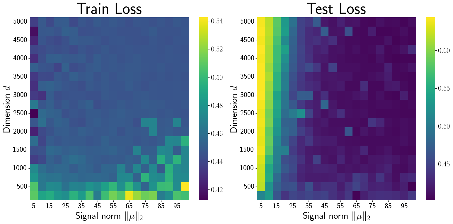
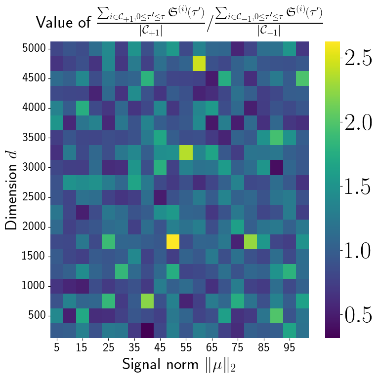
In this section, we provide the results of the additional experiments. Figure 6 shows the train and test loss when varying the dimension and the signal norm . Figure 6 shows the ratio of each class term in Eq.10, scaled by the number of clean data with the same label. In other words, it shows the following value:
| (276) |
The ratio was approximately in the range of to in the trials conducted under the different values of and ,