On the Implicit Relation between Low-Rank Adaptation and Differential Privacy

Abstract

A significant approach in natural language processing involves large-scale pre-training on general domain data followed by adaptation to specific tasks or domains. As models grow in size, full fine-tuning all parameters becomes increasingly impractical. To address this, some methods for low-rank task adaptation of language models have been proposed, e.g. LoRA and FLoRA. These methods keep the pre-trained model weights fixed and incorporate trainable low-rank decomposition matrices into some layers of the transformer architecture, called adapters. This approach significantly reduces the number of trainable parameters required for downstream tasks compared to full fine-tuning all parameters. In this work, we look at low-rank adaptation from the lens of data privacy. We show theoretically that the low-rank adaptation used in LoRA and FLoRA is equivalent to injecting some random noise into the batch gradients w.r.t the adapter parameters coming from their full fine-tuning, and we quantify the variance of the injected noise. By establishing a Berry-Esseen type bound on the total variation distance between the noise distribution and a Gaussian distribution with the same variance, we show that the dynamics of LoRA and FLoRA are very close to differentially private full fine-tuning the adapters, which suggests that low-rank adaptation implicitly provides privacy w.r.t the fine-tuning data. Finally, using Johnson-Lindenstrauss lemma, we show that when augmented with gradient clipping, low-rank adaptation is almost equivalent to differentially private full fine-tuning adapters with a fixed noise scale.

1 Introduction

Stochastic Gradient Descent (SGD) is the power engine of training deep neural networks, which updates parameters of a model by using a noisy estimation of the gradient. Modern deep learning models, e.g. GPT-3 (Brown et al., 2020) and Stable Diffusion (Rombach et al., 2022), have a large number of parameters, which induces a large space complexity for their training with SGD. Using more advanced methods, which track various gradient statistics to stabilize and accelerate training, exacerbates this space complexity (Duchi et al., 2011). For instance, momentum technique reduces variance by using an exponential moving average of gradients (Cutkosky and Orabona, 2019). Also, gradient accumulation (Wang et al., 2013) reduces variance by computing the average of gradients in the last few batches, which simulates a larger effective batch size. All these methods suffer from high space complexity during training/fine-tuning time.

Addressing the space complexity, some works try to reduce it by training a subset of parameters, and storing the information about only a portion of the existing parameters (Houlsby et al., 2019; Ben Zaken et al., 2022). LoRA is such an algorithm, which only updates some of the parameter matrices (called adapters), by restricting their update to be a low-rank matrix. This low-rank restriction considerably reduces the number of trainable parameters, at the cost of limiting the optimization space of the adapter parameters. Another parameter-efficient training technique, called ReLoRA (Lialin et al., 2023), utilizes low-rank updates to train high-rank networks to eliminate the constraint of LoRA mentioned above. Similarly, the work in (Hao et al., 2024) identifies that the dynamics of LoRA can be approximated by a random matrix projection. Based on this interesting finding, the work proposes to achieve high-rank updates by resampling the random projection matrices, while still enjoying the sublinear space complexity of LoRA.

On the other hand, from the lens of data privacy, the fine-tuning data often happens to be privacy sensitive. In such scenarios, Differentially Private (DP) fine-tuning algorithms have been used to provide rigorous privacy guarantees w.r.t the data. DP full fine-tuning runs DPSGD (Abadi et al., 2016) on the the fine-tuning data to update all the existing parameters in a model. However, due to the necessity of computing gradients and clipping them for every data sample, DPSGD also induces high space complexities, even worse than non-private full fine-tuning of all parameters. Despite this, DPSGD full fine-tuning provides rigorous privacy guarantees w.r.t the fine-tuning data.

In this work, we draw a connection between LoRA/FLoRA and DP full fine-tuning the adapters. We show that the random projection existing in the dynamics of LoRA/FLoRA is equivalent to injecting some random noise to the batch gradients coming from full fine-tuning adapters, which is very close to what DPSGD does for full fine-tuning adapters privately. We also quantify the variance of the injected noise, and show that it increases as the rank of adaptation decreases: the smaller the rank of adaptation, the larger the variance of the injected noise. Furthermore, in order to evaluate the closeness of this injected noise to Gaussian noise with the same variance, we bound the total variation (TV) distance between the distribution of the injected noise and the pure Gaussian noise used in DPSGD and show that this bound (dissimilarity) decreases as the rank used in LoRA/FLoRA increases. Our derivations suggest that, although not being exactly the same, low-rank adaptation and DP full fine-tuning adapters are very close to each other in terms of their dynamics. This implies that, besides reducing the space complexity for task adaptation of language models, low rank adaptation can provide privacy w.r.t the fine-tuning data implicitly without inducing the high space complexity of DP full-fine tuning all parameters.

The highlights of our contributions are the followings:

• We show that low-rank adaptation with LoRA/FLoRA is equivalent to injection of some random noise into the adapters’ batch gradients coming from their full fine-tuning (section 3).

• We find the variance of the noise injected into each row of the adapters’ full gradient matrix, and show that it approaches a Gaussian distribution as the number of inputs of the adaptation layer and the adaptation rank increase (lemma 3.1).

• We bound the total variation distance between the distribution of the injected noise and the pure Gaussian noise with the same mean and variance. The bound decreases as the number of inputs of the adaptation layer and the adaptation rank increase (lemma 4.2).

• Finally, we show that the dynamics of low-rank adaptation is very close to DP full fine-tuning adapters, and when it is augmented with gradient clipping, they are almost the same. This implies an implicit connection between LoRA/FLoRA and DPSGD: they are very close to DPSGD with a fixed noise scale, which depends on the adaptation rank, and the batch size used during fine-tuning (section 5).

2 Dynamics of Low-Rank Task Adaptation

We start by studying the dynamics of low-rank adaptation, and restate some of the findings in (Hao et al., 2024). In order to update a pre-trained adapter weight $W\in\mathbb{R}^{n\times m}$, LoRA incorporates low-rank decomposition matrices $B\in\mathbb{R}^{n\times r}$ and $A\in\mathbb{R}^{r\times m}$, where $r\ll\min\{n,m\}$, and performs the forward pass in an adapter layer as:

$$y=(W+BA)x=Wx+BAx,$$ (1)

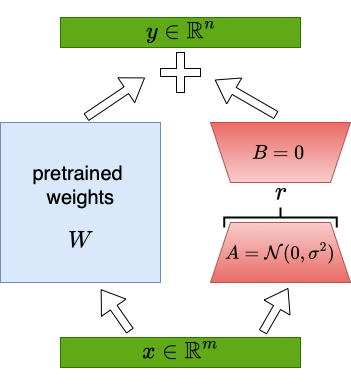
Figure 1: Low-rank decomposition of LoRA/FLoRA for task adaptation.

where $x\in\mathbb{R}^{m}$ is the input of the current layer and $y\in\mathbb{R}^{n}$ is the pre-activation output of the current layer (see fig. 1). It is common to initialize $B$ with an all-zero matrix and $A$ with a normal distribution. More specifically, the entries of $A$ are sampled from $\mathcal{N}(0,\sigma^{2})$ with $\sigma^{2}=\frac{1}{r}$. When back-propagating, gradient of the used loss function $\mathcal{L}$ w.r.t the matrix $W$ is

$$\nabla_{W}\mathcal{L}=\frac{\partial\mathcal{L}}{\partial y}\cdot\frac{\partial y}{\partial W}=\frac{\partial\mathcal{L}}{\partial y}\cdot x^{\top},$$ (2)

where $\frac{\partial\mathcal{L}}{\partial y}\in\mathbb{R}^{n\times 1}$ and $x^{\top}\in\mathbb{R}^{1\times m}$. However, LoRA calculates the gradients w.r.t only A and B, which can be found as follows:

$$\frac{\partial\mathcal{L}}{\partial A}=\frac{\partial BA}{\partial A}\cdot\frac{\partial\mathcal{L}}{\partial BA}=B^{\top}\cdot\frac{\partial\mathcal{L}}{\partial y}\cdot\frac{\partial y}{\partial BA}=B^{\top}\cdot\frac{\partial\mathcal{L}}{\partial y}\cdot x^{\top}=B^{\top}(\nabla_{W}\mathcal{L}).$$ (3)

Similarly,

$$\frac{\partial\mathcal{L}}{\partial B}=\frac{\partial\mathcal{L}}{\partial BA}\cdot\frac{\partial BA}{\partial B}=\frac{\partial\mathcal{L}}{\partial y}\cdot\frac{\partial y}{\partial BA}\cdot A^{\top}=\frac{\partial\mathcal{L}}{\partial y}\cdot x^{\top}\cdot A^{\top}=(\nabla_{W}\mathcal{L})A^{\top}.$$ (4)

Hence, $\frac{\partial\mathcal{L}}{\partial A}\in\mathbb{R}^{r\times m}$ and $\frac{\partial\mathcal{L}}{\partial B}\in\mathbb{R}^{n\times r}$. As observed in eq. 3 and eq. 4 and discussed in (Hao et al., 2024), LoRA down-projects the full gradient $\nabla_{W}\mathcal{L}$ from $\mathbb{R}^{n\times m}$ to a lower dimension, and updates the matrices $A$ and $B$ with the resulting projections of $\nabla_{W}\mathcal{L}$. In fact, it was found in (Hao et al., 2024) that LoRA recovers the well-known random projection method (Dasgupta, 2000; Bingham and Mannila, 2001). We restate the following thorem from (Hao et al., 2024) without restating the proof:

Theorem 2.1 ((Hao et al., 2024), Theorem 2.1).

Let LoRA update matrices $A$ and $B$ with SGD for every step $t$ by

$$A^{t+1}\leftarrow A^{t}-\eta\frac{\partial\mathcal{L}}{\partial A^{t}}=A^{t}-\eta B^{t}{{}^{\top}}(\nabla_{W}\mathcal{L}^{t}),$$ (5)

$$B^{t+1}\leftarrow B^{t}-\eta\frac{\partial\mathcal{L}}{\partial B^{t}}=B^{t}-\eta(\nabla_{W}\mathcal{L}^{t})A^{t}{{}^{\top}},$$ (6)

where $\eta$ is the learning rate. We assume $\|\sum_{t=0}^{T}\nabla_{W}\mathcal{L}^{t}\|_{F}\leq L$ for every $T$ during training, which implies that the model stays within a finite Euclidean ball. In this case, the dynamics of $A^{t}$ and $B^{t}$ are given by

$$A^{t}=A^{0}+\eta A^{0}f_{A}(t),\leavevmode\nobreak\ \leavevmode\nobreak\ \leavevmode\nobreak\ B^{t}=\eta f_{B}(t)A^{0}{{}^{\top}},$$ (7)

where the forms of $f_{A}(t)\in\mathbb{R}^{m\times m}$ and $f_{B}(t)\in\mathbb{R}^{n\times m}$ are expressed in the proof. In particular, $\|f_{A}(t)\|_{2}\leq\frac{\eta L^{2}\big{(}1-(\eta^{2}L^{2})^{t}\big{)}}{1-\eta^{2}L^{2}}$ for every $t$.

Let’s denote the total changes of $A$ and $B$ after $T$ steps as $\Delta A$ and $\Delta B$, respectively. Then, the forward pass eq. 1 changes to:

$$\big{(}W+(B^{0}+\Delta B)(A^{0}+\Delta A)\big{)}x=\big{(}W+\Delta BA^{0}+\Delta B\Delta A\big{)}x,$$ (8)

where we have substituted $B^{0}=\mathbf{0}\in\mathbb{R}^{n\times r}$. From eq. 7 and substituting the values of $\Delta A$ and $\Delta B$ after $T$ rounds of updating $A$ and $B$, we have:

$$W+\Delta BA^{0}+\Delta B\Delta A=W+\eta f_{B}(T)A^{0}{{}^{\top}}A^{0}+\eta^{2}f_{B}(T)A^{0}{{}^{\top}}A^{0}f_{A}(T).$$ (9)

Also, from theorem 2.1, we have $\|f_{A}(T)\|_{2}\leq\|f_{A}(T)\|_{F}\leq\frac{\eta L^{2}\big{(}1-(\eta^{2}L^{2})^{T}\big{)}}{1-\eta^{2}L^{2}}$, for every $T$. Hence, if $\eta\ll 1/L$, we have $\lim_{T\to\infty}\eta\|f_{A}(T)\|_{2}=\lim_{T\to\infty}\frac{(\eta L)^{2}\big{(}1-(\eta L)^{(2T)}\big{)}}{1-(\eta L)^{2}}\ll 1$. Therefore, the last term in eq. 9 is significantly smaller than the second term. Hence, the second term dominates the final update weight. Therefore, as suggested in (Hao et al., 2024) and confirmed with their experimental results, we can closely approximate LoRA by freezing $A$ at its initialized value $A^{0}$ and training only the matrix $B$. In this case,

$$W+\Delta BA^{0}+\Delta B\Delta A =W+\Delta BA^{0}=W+\eta\tilde{f}_{B}(T)A^{0}{{}^{\top}}A^{0},$$ (10)

where $\tilde{f}_{B}(0)=\mathbf{0}$ and $\tilde{f}_{B}(t+1)=\tilde{f}_{B}(t)-\nabla_{W}\mathcal{L}^{t}$. Equivalently, $\tilde{f}_{B}(T)=-\sum_{t=0}^{T-1}\nabla_{W}\mathcal{L}^{t}$. Substituting this into the equation above, we get:

$$W+\Delta BA^{0}+\Delta B\Delta A=W+\Delta BA^{0}=W-\eta\sum_{t=0}^{T-1}\big{[}(\nabla_{W}\mathcal{L}^{t})A^{0}{{}^{\top}}A^{0}\big{]},$$ (11)

where the last term shows the exact parameter change after $T$ rounds of performing SGD on the adapter matrix $B$. Therefore, low rank adaptation with LoRA can be viewed as performing a random projection of stochastic batch gradient $\nabla_{W}\mathcal{L}^{t}$ in every step $t$ by matrix $A^{0}{{}^{\top}}$ and projecting it back by matrix $A^{0}$. FLoRA (Hao et al., 2024) proposes to resample the random matrix $A^{0}$ at each step to get a high rank update $\Delta B$ for the matrix $B$. Hence, FLoRA can also be viewed as performing a random projection of stochastic batch gradient $\nabla_{W}\mathcal{L}^{t}$ in every step $t$ by a different random matrix $A{{}^{\top}}$ and projecting it back by its transpose.

Having understood the connection between low-rank adaptation in LoRA/FLoRA and random projection, in the next section, we show that this random projection and back projection performed in each time step is equivalent to adding some random noise to each element of $\nabla_{W}\mathcal{L}^{t}$. This is our first step towards establishing the connection between low-rank adaptation and differential privacy.

3 Random Noise Injected by Low-Rank Adaptation

In this section, we present our analysis based on LoRA, which employs a fixed projection matrix $A^{0}$. Our analysis holds for various LoRA variants, including FLoRA. As illustrated in section 3, the parameter update after $T$ rounds of stochastic gradient descent (SGD) is given by:

$$W+\Delta BA^{0}+\Delta B\Delta A =W-\eta\sum_{t=0}^{T-1}\bigg{[}(\nabla_{W}\mathcal{L}^{t})A^{0}{{}^{\top}}A^{0}\bigg{]}$$

$$=W-\eta\sum_{t=0}^{T-1}\bigg{[}\underbrace{\nabla_{W}\mathcal{L}^{t}}_{\textit{full fine-tuning}}\underbrace{-\nabla_{W}\mathcal{L}^{t}(A^{0}{{}^{\top}}A^{0}-\mathbb{I}_{m})}_{\textit{noise}\leavevmode\nobreak\ \in\leavevmode\nobreak\ \mathbb{R}^{n\times m}}\bigg{]},$$ (12)

The first term in the sum represents the batch gradient that would be obtained through full fine-tuning the adapter $W$. The second term represents the noise introduced by the low-rank adaptation. Thus, the low-rank adaptation introduces noise to each batch gradient $\nabla_{W}\mathcal{L}^{t}$, and the gradient step is taken with this noisy gradient. We are now particularly interested in the behavior of this noise term, which is added to each batch gradient $\nabla_{W}\mathcal{L}^{t}$ in every step $t$. Recall that the entries of $A^{0}$ were sampled from $\mathcal{N}(0,\frac{1}{r})$ (see fig. 1), and that each of the $r$ columns of $A^{0}{{}^{\top}}$ is an $m$-dimensional Gaussian random variable. Consequently, $A^{0}{{}^{\top}}A^{0}$ follows a Wishart distribution with $r$ degrees of freedom (Bhattacharya and Burman, 2016), which is the multivariate generalization of the chi-squared distribution. Therefore, for any $q\in\mathbb{R}^{1\times m}$, $q\cdot(A_{0}^{\top}A_{0}-\mathbb{I}_{m})$ is a weighted sum of multiple chi-squared random variables, which implies that the result follows a Gaussian distribution approximately, according to the Central Limit Theorem (CLT) (Bhattacharya et al., 2016). We prove the following lemma concerning the noise term in section 3.

Lemma 3.1.

Let $A\in\mathbb{R}^{r\times m}$ be a matrix with i.i.d entries sampled from $\mathcal{N}(0,\frac{1}{r})$. Given a fixed $q\in\mathbb{R}^{1\times m}$, the distributions of elements of $q\cdot(A^{\top}A-\mathbb{I}_{m})\in\mathbb{R}^{1\times m}$ approach the Gaussian distribution $\mathcal{N}(0,\frac{\|q\|^{2}}{r})$, as $m$ approaches infinity.

The result above can be extended to matrices multiplication, as in section 3: for a matrix $Q\in\mathbb{R}^{n\times m}$ and as $m\to\infty$, the product $G=Q\cdot(A^{\top}A-\mathbb{I}_{m})\in\mathbb{R}^{n\times m}$ approaches a Gaussian distribution, where $G_{i,j}$ ($1\leq i\leq n$) has distribution $\mathcal{N}(0,\frac{\|[Q]_{i,:}\|^{2}}{r})$, where $[Q]_{i,:}$ is the $i$-th row of $Q$. The lemma above shows that the last term in section 3 can indeed be looked at as a random noise term with mean $0$ and a variance depending on $\nabla_{w}\mathcal{L}^{t}$.

Although lemma 3.1 was proved for when $m$ approaches infinity, in practical scenarios it is limited. Hence, the distribution of the injected noise in not pure Gaussian. In the next section, we bound the deviation of the noise distribution from a pure Gaussian distribution.

4 Bounding the Distance to the Normal Law

Despite having proved lemma 3.1 when $m$ approaches infinity, yet we need to quantify the distance between the distribution of $q\cdot(A^{\top}A-\mathbb{I}_{m})\in\mathbb{R}^{1\times m}$ to the bona fide Gaussian distribution for limited values of $m$ in practical scenarios. In this section, we derive a closed form upper-bound for the total variation distance between the distribution of each element of $q\cdot(A^{\top}A-\mathbb{I}_{m})\in\mathbb{R}^{1\times m}$ and the Gaussian distribution with the same mean and variance.

Consistent with the notations in Theorem A.4 in the appendix, suppose $X_{1},\ldots,X_{n}$ are $n$ independent random variables with $\mathbb{E}[X_{i}]=0$ and $\texttt{Var}[X_{i}]=\sigma_{i}^{2}>0$. Define $S_{n}=\sum_{i=1}^{n}X_{i}$ and let $s_{n}^{2}=\sum_{i=1}^{n}\sigma_{i}^{2}$. Assuming $Z_{n}=\frac{S_{n}}{s_{n}}$, and having Lindeberg’s condition satisfied (see theorem A.3 and theorem A.4), the normalized sum $Z_{n}$ has standard normal distribution in a weak sense for a bounded $n$. More precisely, the closeness of the cumulative distribution function (CDF) $F_{n}(x)=\texttt{Pr}\{Z_{n}\leq x\}$ to the standard normal CDF

$$\Phi(x)=\frac{1}{\sqrt{2\pi}}\int_{-\infty}^{x}e^{-\frac{y^{2}}{2}}dy$$ (13)

has been studied intensively in terms of the Lyapounov ratios

$$L_{t}=\frac{\sum_{i=1}^{n}\mathbb{E}[|X_{i}|^{t}]}{s_{n}^{t}}.$$ (14)

Particularly, if all $X_{i}$ have a finite third absolute moment $\mathbb{E}[|X_{i}|^{3}]$, the classical Berry-Esseen theorem bounds the Kolmogrov distance between $F_{n}(x)$ and $\Phi(x)$:

$$\sup_{x}|F_{n}(x)-\Phi(x)|\leq CL_{3},$$ (15)

where $c$ is an absolute constant (see (gustav Esseen, 1945; Feller, 1971; Petrov, 1975)). In the general case of sum of independent random variables (and not necessarily i.i.d random variables), which we are interested in, the number of summand variables $n$ implicitly affects the value of $L_{3}$. For the sum of independent random variables, the work in (Bobkov et al., 2011) bounds the difference between $F_{n}(x)$ and $\Phi(x)$ in terms of generally stronger distances of total variation and entropic distances. Considering the $X_{i}$ above, let $D(X_{i})$ denote the KL divergence between distribution of $X_{i}$ and Gaussian distribution $\mathcal{N}(0,\sigma_{i}^{2})$, i.e. the KL divergence between $X_{i}$ and a Gaussian with the same variance. We have the following theorem about the total variation distance between $F_{n}$ and $\Phi$:

Theorem 4.1 ((Bobkov et al., 2011), theorem 1.1).

Assume that the independent random variables $X_{1},\ldots,X_{n}$ have finite third absolute moments, and that $D(X_{i})\leq D$, where $D$ is a non-negative number. Then,

$$\|F_{n}(x)-\Phi(x)\|_{TV}\leq C_{D}L_{3},$$ (16)

where the constant $C_{D}$ depends on $D$ only and $\|F_{n}(x)-\Phi(x)\|_{TV}=\sup_{A}\big{|}\int_{A}dF_{n}-\int_{A}d\Phi\big{|}$ is the total variation distance between $F_{n}$ and $\Phi$.

Having the theorem above, we can derive a Berry-Esseen type bound for the total variation distance between each element of $q\cdot(A^{\top}A-\mathbb{I}_{m})\in\mathbb{R}^{1\times m}$ in lemma 3.1 and the normal law $\mathcal{N}(0,\frac{\|q\|^{2}}{r})$: we need to find the third Lyapounov ratio for the summands contributing to each element, as in eq. 16. To this end, we state and prove the following lemma:

Lemma 4.2.

Let $A\in\mathbb{R}^{r\times m}$ be a matrix with i.i.d entries sampled from $\mathcal{N}(0,\frac{1}{r})$. Given a fixed $q\in\mathbb{R}^{1\times m}$ with elements $0<c\leq|q_{i}|\leq C$, let $u=q\cdot(A^{\top}A-\mathbb{I}_{m})\in\mathbb{R}^{1\times m}$. Let $u_{i}$ be the $i$-th element of $u$ and $Q_{m}(x)=\texttt{Pr}\{u_{i}\leq x\}$. Also, let $\Phi(x)$ be the CDF of normal variable $z\sim\mathcal{N}(0,\frac{\|q\|^{2}}{r})$. Then:

$$\|Q_{m}(x)-\Phi(x)\|_{TV}\in\mathcal{O}\bigg{(}\frac{1}{\sqrt{mr}}\bigg{)}.$$ (17)

The lemma above states that the distribution of each element of $q\cdot(A^{\top}A-\mathbb{I}_{m})\in\mathbb{R}^{1\times m}$ approaches to $\mathcal{N}(0,\frac{\|q\|^{2}}{r})$ with rate $\frac{1}{\sqrt{mr}}$ in terms of their total variation distance. This result shows the elements of $q\cdot(A^{\top}A-\mathbb{I}_{m})\in\mathbb{R}^{1\times m}$ approach to Gaussian $\mathcal{N}(0,\frac{\|q\|^{2}}{r})$ as $m$ and $r$ increase. Having the interesting result above, we can now benefit from the useful coupling characterization of the total variation distance to establish a more understandable relation between each element of the product above and the Gaussian distribution $\mathcal{N}(0,\frac{\|q\|^{2}}{r})$.

The coupling characterization of the total variation distance.

For two distributions $P$ and $Q$, a pair of random variables $(X,Y)$, which are defined on the same probability space, is called a coupling for $P$ and $Q$ if $X\sim P$ and $Y\sim Q$ (Levin et al., 2008; Devroye et al., 2023). A very useful property of total variation distance is the coupling characterization:

$\|P-Q\|_{TV}\leq t$ if and only if there exists a coupling $(X,Y)$ for them such that $\texttt{Pr}\{X\neq Y\}\leq t$ (see proposition 4.7 in (Levin et al., 2008)).

Hence, we can use the coupling characterization above and get to the following lemma directly from from lemma 4.2.

Lemma 4.3.

Let $A\in\mathbb{R}^{r\times m}$ be a matrix with i.i.d entries sampled from $\mathcal{N}(0,\frac{1}{r})$. Given a fixed $q\in\mathbb{R}^{1\times m}$ with elements $0<c\leq|q_{i}|\leq C$, let $u=q\cdot(A^{\top}A-\mathbb{I}_{m})\in\mathbb{R}^{1\times m}$. Let $u_{i}$ be the $i$-th element of $u$. Then there exists a coupling $(u_{i},z)$, where $z\sim\mathcal{N}(0,\frac{\|q\|^{2}}{r})$ and

$$\texttt{Pr}\{u_{i}\neq z\}\in\mathcal{O}\bigg{(}\frac{1}{\sqrt{mr}}\bigg{)}.$$ (18)

The lemma above means that each element $u_{i}$ follows a mixture of distributions: $\mathcal{N}(0,\frac{\|q\|^{2}}{r})$ with weight $w_{g}$ and another distribution $M$, which we dont know, with weight $(1-w_{g})\in\mathcal{O}\big{(}\frac{1}{\sqrt{mr}}\big{)}$. The larger $mr$, the closer the mixture distribution gets to pure Gaussian distribution $\mathcal{N}(0,\frac{\|q\|^{2}}{r})$. Having the results above, we can now draw a clear connection between low-rank adaptation and DP.

5 Connecting Low Rank Adaptation to DP with Gradient Clipping

Based on section 3 and our understandings from lemma 4.3, low rank adaptation (with rank $r$) of adapter parameter $W\in\mathbb{R}^{n\times m}$ at time step $t$ is equivalent to full fine-tuning it with the noisy stochastic batch gradients $\tilde{\nabla}_{W}\mathcal{L}^{t}=\nabla_{W}\mathcal{L}^{t}+N^{t}$, where $N^{t}\in\mathbb{R}^{n\times m}$ is a noise-term with Gaussian-like distribution: $\texttt{Pr}\{N_{i,j}^{t}\neq z_{i}^{t}\}\in\mathcal{O}\big{(}\frac{1}{\sqrt{mr}}\big{)}$, where $z_{i}^{t}\sim\mathcal{N}(0,\frac{\|[\nabla_{W}\mathcal{L}^{t}]_{i,:}\|^{2}}{r})$, and $[\nabla_{W}\mathcal{L}^{t}]_{i,:}$ is the $i$-th row of $\nabla_{W}\mathcal{L}^{t}$ ($1\leq i\leq n$). Asymptotically, as $mr$ grows, i.e. the input dimension of the adaptation layer ($m$) increases or the adaptation rank increases ($r<m$), the distribution of noise element $N_{i,j}^{t}$ gets closer to $\mathcal{N}(0,\frac{\|[\nabla_{W}\mathcal{L}^{t}]_{i,:}\|^{2}}{r})$. In other words, low-rank adaptation adds noise to each row of batch gradient $\nabla_{W}\mathcal{L}^{t}$, and the standard deviation of the noise added to the elements of the row $i$ is proportional to the $\ell_{2}$ norm of row $i$. This operation is very similar to what DPSGD (Abadi et al., 2016) does for adding noise to each element of the batch gradients w.r.t the adapter parameters: at the $t$-th gradient update step on a current adapter parameter $W$, DPSGD computes the following noisy batch gradient on a batch of size $b$:

$$\tilde{\nabla}_{W}\mathcal{L}^{t}=\frac{1}{b}\bigg{[}\Big{(}\sum_{i\in\mathcal{B}^{t}}\bar{\nabla}_{W}\mathcal{L}_{i}^{t}\Big{)}+\mathcal{N}(0,\sigma_{\texttt{DP}}^{2})\bigg{]},$$ (19)

where $\bar{\nabla}_{W}\mathcal{L}_{i}^{t}=\texttt{clip}(\nabla_{W}\mathcal{L}_{i}^{t},c)$, $c$ is a clipping threshold, and $\mathcal{B}^{t}$ is the batch of samples at time step $t$. Also, $\sigma_{\texttt{DP}}=c\cdot z$, where $z$ is the noise scale determining the resulting privacy guaranty parameters. The main difference between the noise addition mechanism in low-rank adaptation (section 3) and that in DPSGD (eq. 19) is that DPSGD adds noise with a fixed variance $\sigma_{\texttt{DP}}^{2}$ to all elements of the clipped batch gradient, and also there is no sample gradient clipping happening in low rank adaptation. In the following, we show that how this clipping can be introduced in low rank adaptation with almost no cost by using Johnson-Lindenstrauss Lemma. This also leads to the same noise variance for all elements. We first state a version of the lemma in the following.

Theorem 5.1 ((Matousek, 2008), Theorem 3.1).

Let $m$ be an integer, $\Delta\in(0,\frac{1}{2}]$, and $p\in(0,1)$. Also, let us set $r=\Delta^{-2}log(\frac{p}{2})$. Let us define a random linear map $T:\mathbb{R}^{m}\to\mathbb{R}^{r}$ by

$$T(x)_{i}=\frac{1}{\sqrt{r}}\sum_{j=1}^{m}R_{ij}x_{j},\leavevmode\nobreak\ \leavevmode\nobreak\ \leavevmode\nobreak\ i=1,\cdots,r$$ (20)

where the $R_{ij}$ are independent standard normal variables. Then for every $x\in\mathbb{R}^{m}$, we have:

$$\texttt{Pr}[(1-\Delta)\|x\|\leq\|T(x)\|\leq(1+\Delta)\|x\|]\geq 1-p.$$ (21)

or equivalently

$$\texttt{Pr}\bigg{[}\frac{\|T(x)\|}{(1+\Delta)}\leq\|x\|\leq\frac{\|T(x)\|}{(1-\Delta)}\bigg{]}\geq 1-p.$$ (22)

The theorem above directly relates to the random projection mapping $A^{\top}$ observed in LoRA/FLoRA: let us define the mapping $T$ in theorem 5.1 to be $T(x)=xA^{\top}$. Then we know that for a sample $i$ in a batch of samples with size $b$, $\nabla_{B^{t}}\mathcal{L}_{i}^{t}=T(\nabla_{W^{t}}\mathcal{L}_{i}^{t})$. Therefore, if we clip a row $l$ of $\nabla_{B^{t}}\mathcal{L}_{i}^{t}$ with a clipping threshold, it is almost equivalent to clipping the same row of $\nabla_{W^{t}}\mathcal{L}_{i}^{t}$ with the same clipping threshold. More precisely, let’s fix $\Delta$. Then, according to eq. 22, for every sample $i$ in a batch $\mathcal{B}^{t}$ and every row $l\in[1,n]$, we have:

$$\big{\|}[\nabla_{B^{t}}\mathcal{L}_{i}^{t}]_{l,:}\big{\|}=(1-\Delta)\sqrt{r}c\leavevmode\nobreak\ \Rightarrow\leavevmode\nobreak\ \texttt{Pr}\bigg{[}\frac{(1-\Delta)}{(1+\Delta)}\sqrt{r}c\leq\big{\|}[\nabla_{W^{t}}\mathcal{L}_{i}^{t}]_{l,:}\big{\|}\leq\sqrt{r}c\bigg{]}\geq 1-p,$$ (23)

where $r=\Delta^{-2}\log(\frac{2}{p})$. Therefore, if the left condition is satisfied for all samples $i$ in a batch of size $b$ and all rows $l$, then with probability at least $(1-nbp)$, the right bound holds for all samples $i$ and rows $l$. Equivalently, we have the following :

$$\big{\|}[\nabla_{B^{t}}\mathcal{L}_{i}^{t}]_{l,:}\big{\|}=(1-\Delta)\sqrt{r}c\leavevmode\nobreak\ \leavevmode\nobreak\ \leavevmode\nobreak\ (\forall\leavevmode\nobreak\ l,i)\Rightarrow\texttt{Pr}\bigg{[}\frac{(1-\Delta)}{(1+\Delta)}\sqrt{nr}c\leq\|\nabla_{W^{t}}\mathcal{L}_{i}^{t}\|_{F}\leq\sqrt{nr}c\bigg{]}\geq 1-nbp,$$ (24)

for all samples $i$ in a batch of size $b$. In other words, if we clip all the rows of sample gradients $\nabla_{B^{t}}\mathcal{L}_{i}^{t}$ in a batch to have norm $(1-\Delta)\sqrt{r}c$, then with probability at least $1-nbp$, all the sample gradients $\nabla_{W^{t}}\mathcal{L}_{i}^{t}$ in a batch have bounded frobenious norm $\sqrt{nr}c$. In that case, according to lemma 3.1, low rank adaptation of LoRA/FLoRA adds a random noise to each row of $\nabla_{W^{t}}\mathcal{L}_{i}^{t}$ based on the norm of the row. More precisely, low-rank adaptation adds a Gaussian-like noise with variance at least $\frac{(\frac{(1-\Delta)}{(1+\Delta)}\sqrt{r}c)^{2}}{r}=\frac{(1-\Delta)^{2}}{(1+\Delta)^{2}}c^{2}$ to each element of the clipped sample gradient $\nabla_{W^{t}}\mathcal{L}_{i}^{t}$, whose frobenious norm was bounded in eq. 24. Also, according to lemma 4.3, the noise added to each element follows Gaussian distribution $\mathcal{N}(0,\frac{(1-\Delta)^{2}}{(1+\Delta)^{2}}c^{2})$ with probability $w_{g}$, where $(1-w_{g})\in\mathcal{O}\big{(}\frac{1}{\sqrt{mr}}\big{)}$.

5.1 Connecting LoRA/FLoRA to DPSGD Algorithm

As described above, when augmented with clipping of the rows of sample gradients $\nabla_{B^{t}}\mathcal{L}_{i}^{t}\leavevmode\nobreak\ (i\in\mathcal{B}^{t})$, the dynamics of LoRA/FLoRA is very close to DPSGD. However, it is not exactly the same: first, the distribution that the injected noise is sampled from is not exactly the pure Gaussian $\mathcal{N}(0,\frac{(1-\Delta)^{2}}{(1+\Delta)^{2}}c^{2})$. Second, as seen in eq. 24, the gradient clipping is probabilistic, while in DPSGD, the sample gradient clipping is deterministic, as if $p=0$ in eq. 24. Despite this, we can think of an intuitive relation to DPSGD. If we assume that the noise distribution is very close to Gaussian distribution (i.e. $w_{g}\approx 1$), and also $nbp\ll 1$, then we can consider the following interpretation of the low-rank adaptation of LoRA/FLoRA:

When clipping all the rows of sample gradients $\nabla_{B^{t}}\mathcal{L}_{i}^{t}$ to have norm $(1-\Delta)\sqrt{r}c$, low-rank adaptation adds a Gaussian noise with variance at least $(\frac{(1-\Delta)}{(1+\Delta)}\sqrt{r}c)^{2}/r=\frac{(1-\Delta)^{2}}{(1+\Delta)^{2}}c^{2}$ to each element of the clipped sample gradients $\nabla_{W^{t}}\mathcal{L}_{i}^{t}$, whose frobenious norm is bounded by $\sqrt{nr}c$. This is equivalent to having a noise scale $z\geq\sqrt{b\frac{(1-\Delta)^{2}}{(1+\Delta)^{2}}c^{2}}/\sqrt{nr}c=\frac{(1-\Delta)}{(1+\Delta)}\sqrt{\frac{b}{nr}}$ for each batch of size $b$. The DP privacy parameters $\epsilon$ and $\delta$ resulting from this noise scale, which can be found by using a privacy accountant, e.g. moments accountant (Abadi et al., 2016), depend on the used batch size ratio (ratio of the batch size $b$ and the fine-tuning dataset size) and the number of steps $T$ taken during fine-tuning.

The connection drawn above is an approximate, yet meaningful, connection between LoRA/FLoRA and DPSGD, which provides a clear interpretation of what low-rank adaptation does. In fact, low-rank adaptation secretly approximates the mechanism of DPSGD during fine-tuning. Hence, we expect it to provide robustness against privacy attacks to the data used for fine-tuning large models. Indeed, such a behavior for low-rank adaptation has been observed implicitly in (Liu et al., 2024).

6 Conclusion

In this study, we establish an implicit connection between low-rank adaptation and differential privacy. We show that low-rank adaptation can be viewed as introducing random noise into the gradients w.r.t adapters coming from their full fine-tuning. By quantifying the variance of this noise and bounding its deviation from pure Gaussian noise with the same variance, we demonstrate that low-rank adaptation, when combined with gradient clipping, approximates full fine-tuning adapters with differential privacy. Although our theoretical analysis suggests that low-rank adaptation can provide implicit privacy similar to those of full fine-tuning with differential privacy at a lower computational cost, empirical evaluation is necessary to fully validate these claims. In our ongoing future direction, we will explore whether low-rank adaptation can effectively balance data privacy, security, and fine-tuning efficiency. Specifically, we aim to assess the practical performance of low-rank adaptation against security threats such as membership inference attacks (Zarifzadeh et al., 2024; Ye et al., 2022) and secret sharing scenarios (Carlini et al., 2019).

Appendix for on the Implicit Relation between Low-Rank Adaptation and Differential Privacy

Appendix A Useful Theorems

In this section, we mention some theorems, which we will use in our proofs.

Theorem A.1 (Chi-Squared distribution: [Mood and Franklin, 1974], Section 4.3, Theorem 7).

If the random variables $X_{i}$, $i=1,\ldots,k$, are normally and independently distributed with means $\mu_{i}$ and variances $\sigma_{i}^{2}$, then

$$U=\sum_{i=1}^{k}\big{(}\frac{X_{i}-\mu_{i}}{\sigma_{i}}\big{)}^{2}$$ (25)

has a chi-squared distribution with $k$ degrees of freedom: $U\sim\mathcal{X}_{k}^{2}$. Also, $\mathbb{E}[U]=k$ and $\texttt{Var}[U]=2k$.

The theorem above states that sum of the squares of $k$ standard normal random variables is a chi-squared distribution with $k$ degrees of freedom.

Lemma A.2 (Raw moment of Chi-Squared distribution).

Suppose $X\sim\mathcal{X}_{k}^{2}$. Then, the $m$-th raw moment of $X$ can be found as follows;

$$\mathbb{E}[X^{m}]=\prod_{i=0}^{m-1}(k+2i)$$ (26)

Proof.

From the definition of Chi-Squared distribution with $r$ degrees of reddom, $U$ has the following probability density function:

$$f_{X}(x)=\frac{1}{2^{\frac{k}{2}}\Gamma(\frac{k}{2})}x^{\frac{k}{2}-1}e^{-\frac{x}{2}}$$ (27)

Therefore, we have:

$$\mathbb{E}[X^{m}] =\frac{1}{2^{\frac{k}{2}}\Gamma(\frac{k}{2})}\int_{0}^{+\infty}x^{\frac{k}{2}+m-1}e^{-\frac{x}{2}}dx=\frac{2}{2^{\frac{k}{2}}\Gamma(\frac{k}{2})}\int_{0}^{+\infty}(2u)^{\frac{k}{2}+m-1}e^{-u}du$$

$$=\frac{2^{\frac{k}{2}+m-1+1}}{2^{\frac{k}{2}}\Gamma(\frac{k}{2})}\int_{0}^{+\infty}u^{\frac{k}{2}+m-1}e^{-u}du=\frac{2^{m}}{\Gamma(\frac{k}{2})}\Gamma(\frac{k}{2}+m)=\frac{2^{m}\Gamma(\frac{k}{2})}{\Gamma(\frac{k}{2})}\prod_{i=0}^{m-1}(\frac{k}{2}+i)$$

$$=\prod_{i=0}^{m-1}(k+2i).$$ (28)

Note that the fifth equality directly results from the property of gamma function that for $z>0$, $\Gamma(1+z)=z\Gamma(z)$. ∎

Theorem A.3 (Classical Central Limit Theorem: [Billingsley, 1995], Theorem 27.1).

Suppose that $\{X_{i}\}_{i=1}^{n}$, is an independent sequence of random variables having the same distribution with mean $\mu$ and positive variance $\sigma^{2}$. Define $S_{n}=\sum_{i=1}^{n}X_{i}$ as their sum. Let $Z_{n}$ be defined by

$$Z_{n}=\frac{S_{n}-n\mu}{\sqrt{n}\sigma}.$$ (29)

Then, the distribution of $Z_{n}$ approaches standard normal distribution as $n$ approaches infinity.

The theorem above states that $S_{n}$ is approximately, or asymptotically, distributed as a normal distribution with mean $n\mu$ and variance $n\sigma^{2}$.

The next theorem is about the Lindeberg’s condition, which is a sufficient (and under certain conditions also a necessary condition) for the Central Limit Theorem (CLT) to hold for a sequence of independent random variables $\{X_{i}\}_{i=1}^{n}$. Unlike the classical CLT stated above, which requires the sequence of random variables to have a finite variance and be both independent and identically distributed (i.i.d), Lindeberg’s CLT only requires the sequence of random variables to have finite variance, be independent and also satisfy the Lindeberg’s condition. The following states the theorem.

Theorem A.4 (Lindeberg and Lyapounov Theorem: [Billingsley, 1995], Theorem 27.2).

Suppose $X_{1},\ldots,X_{n}$ are $n$ independent random variables with $\mathbb{E}[X_{i}]=\mu_{i}$ and $\texttt{Var}[X_{i}]=\sigma_{i}^{2}>0$. Define $S_{n}=\sum_{i=1}^{n}X_{i}$ and let $s_{n}^{2}=\sum_{i=1}^{n}\sigma_{i}^{2}$. Also assume the following condition holds for all $\epsilon>0$:

$$\textit{Lindeberg's condition:}\leavevmode\nobreak\ \leavevmode\nobreak\ \leavevmode\nobreak\ \lim_{n\to\infty}\sum_{i=1}^{n}\frac{1}{s_{n}^{2}}\int_{|x-\mu_{i}|\geq\epsilon s_{n}}(x-\mu_{i})^{2}P_{X_{i}}(x)dx=0.$$ (30)

where $P_{X_{i}}$ is the pdf of variable $X_{i}$. Assuming $Z_{n}=\frac{S_{n}-\sum_{i=1}^{n}\mu_{i}}{s_{n}}$, the distribution of $Z_{n}$ approaches standard normal distribution as $n$ approaches infinity.

The theorem above states that, given that Lindeberg’s condition is satisfied, $S_{n}$ is approximately, or asymptotically, distributed as a normal distribution with mean $\sum_{i=1}^{n}\mu_{i}$ and variance $s_{n}^{2}$, even if the sequence of variables are not identically distributed.

Appendix B Proofs

Using the theorems above, we are now able to prove lemma 3.1. See 3.1

Proof.

From the theorem’s assumption, we know that elements of $A$ are from $\mathcal{N}(0,\frac{1}{r})$. Therefore, we can rewrite the product $q\cdot(A^{\top}A-\mathbb{I}_{m})\in\mathbb{R}^{1\times m}$ as the following product:

$$q\cdot(\frac{A^{\top}A}{r}-\mathbb{I}_{m})\in\mathbb{R}^{1\times m}$$ (31)

where the elements of $A$ are now from standard normal distribution. Let $a_{i,j}$ denote the element in $i$-th row and $j$-th column of this new $A$. Therefore, for all $i$ and $j$, $a_{i,j}$ has distribution $\mathcal{N}(0,1)$. Let $B=\frac{A^{\top}A}{r}-\mathbb{I}_{m}$. Also, let $A_{i,:}$ and $A_{:,j}$ denote the $i$-th row and $j$-th column of the new $A$, respectively. We have:

$$B_{i,i}=\frac{1}{r}[A^{\top}A]_{i,i}-1=\frac{1}{r}A_{:,i}^{\top}A_{:,i}-1=\frac{1}{r}\|A_{:,i}\|_{2}^{2}-1=(\frac{1}{r}\sum_{l=1}^{r}a_{l,i}^{2})-1$$ (32)

From eq. 31, we know that $a_{l,i}$ is from standard normal distribution. Hence, $a_{l,i}^{2}$ is a chi-squared with 1 degree of freedom: $a_{l,i}^{2}\sim\mathcal{X}_{1}^{2}$. Therefore, $\sum_{l=1}^{r}a_{l,i}^{2}$, which is the sum of $r$ independent chi-squared variables with 1 degree of freedom, is a chi-squared with $r$ degrees of freedom: $\sum_{l=1}^{r}a_{l,i}^{2}\sim\mathcal{X}_{r}^{2}$ (see theorem A.1). Therefore, for $i\in\{1,\ldots,m\}$, we have:

$$\mathbb{E}[B_{i,i}]=\mathbb{E}\big{[}\frac{\sum_{l=1}^{r}a_{l,i}^{2}}{r}\big{]}-1=\frac{r}{r}-1=0,$$

$$\texttt{Var}[B_{i,i}]=\texttt{Var}[\frac{\sum_{l=1}^{r}a_{l,i}^{2}}{r}]=\frac{\texttt{Var}(\mathcal{X}_{r}^{2})}{r^{2}}=\frac{2r}{r^{2}}=\frac{2}{r}.$$ (33)

Similarly, we find the mean and variance of the non-diagonal elements $B_{i,j}(i\neq j)$ of $B$. We have:

$$B_{i,j}=\frac{1}{r}[A^{\top}A]_{i,j}=\frac{1}{r}A_{:,i}^{\top}A_{:,j}=\frac{1}{r}\sum_{l=1}^{r}a_{l,i}a_{l,j},$$ (34)

where $a_{l,i}$ and $a_{l,j}$ are independent and standard normal. Therefore, $a_{l,i}+a_{l,j}\sim\mathcal{N}(0,2)$. Similarly, $a_{l,i}-a_{l,j}\sim\mathcal{N}(0,2)$. So we can rewrite $a_{l,i}a_{l,j}$ as:

$$a_{l,i}a_{l,j}=\frac{1}{4}(a_{l,i}+a_{l,j})^{2}-\frac{1}{4}(a_{l,i}-a_{l,j})^{2}=\frac{1}{2}z_{1}^{2}-\frac{1}{2}z_{2}^{2},$$ (35)

where $z_{1}$ and $z_{2}$ are from standard normal. Therefore, $a_{l,i}a_{l,j}=\frac{\nu_{1}-\nu_{2}}{2}$, where $\nu_{1},\nu_{2}\sim\mathcal{X}_{1}^{2}$. Also, $a_{l,i}+a_{l,j}$ and $a_{l,i}-a_{l,j}$ are independent variables. Hence, $z_{1}$ and $z_{2}$ are independent, and likewise $\nu_{1}$ and $\nu_{2}$ are independent. We conclude that:

$$a_{l,i}a_{l,j}=\frac{1}{2}(\nu_{1}-\nu_{2}),$$ (36)

where $\nu_{1},\nu_{2}\sim\mathcal{X}_{1}^{2}$, and are independent.

Now, lets assume $\nu_{1},\nu_{2}\sim\mathcal{X}_{k}^{2}$ (a more general case), and let $M_{\nu_{1}}(t)=\mathbb{E}[e^{t\nu_{1}}]$ be the moment generating function (MGF) of $\nu_{1}$. In this case, we know that $M_{\nu_{1}}(t)=M_{\nu_{2}}(t)=(1-2t)^{-\frac{k}{2}}$ (MGF of $\mathcal{X}_{k}^{2}$). Hence, $M_{\nu_{1}-\nu_{2}}(t)=M_{\nu_{1}}(t)\cdot M_{\nu_{2}}(-t)=(1-4t^{2})^{-\frac{k}{2}}=\big{(}\frac{\frac{1}{4}}{\frac{1}{4}-t^{2}}\big{)}^{\frac{k}{2}}$, which is the MGF of a symmetric about origin variance-gamma distribution with parameters $\lambda=\frac{k}{2},\alpha=\frac{1}{2},\beta=0,\mu=0,\gamma=\frac{1}{2}$. Therefore, when $\nu_{1},\nu_{2}\sim\mathcal{X}_{k}^{2}$, then $\nu_{1}-\nu_{2}$ has this distribution, which has mean $\mu+2\beta\lambda/\gamma^{2}=0$ and variance $2\lambda(1+2\beta^{2}/\gamma^{2})/\gamma^{2}=4k$.

In eq. 36, we had $k=1$, as we had $\nu_{1},\nu_{2}\sim\mathcal{X}_{1}^{2}$. Hence, based on the discussion above, we have:

$$\mathbb{E}[a_{l,i}a_{l,j}] =0$$ (37)

$$\texttt{Var}[a_{l,i}a_{l,j}] =\frac{1}{4}\texttt{Var}[\nu_{1}-\nu_{2}]=\frac{4k}{4}=1$$ (38)

Consequently, based on eq. 34 and from the results above, we can compute the mean and variance of the non-diagonal elements of $B$ ($i\neq j$):

$$\mathbb{E}[B_{i,j}]=\mathbb{E}\big{[}\frac{\sum_{l=1}^{r}a_{l,i}a_{l,j}}{r}\big{]}=\frac{\sum_{l=1}^{r}\mathbb{E}[a_{l,i}a_{l,j}]}{r}=0,$$

$$\texttt{Var}[B_{i,j}]=\texttt{Var}[\frac{\sum_{l=1}^{r}a_{l,i}a_{l,j}}{r}]=\frac{\sum_{l=1}^{r}\texttt{Var}[a_{l,i}a_{l,j}]}{r^{2}}=\frac{r}{r^{2}}=\frac{1}{r}.$$ (39)

So far, we have computed the mean and variance of each entry in $B=\frac{A^{\top}A}{r}-\mathbb{I}_{m}\in\mathbb{R}^{m\times m}$ in appendix B and appendix B. Now, for a given $q\in\mathbb{R}^{1\times m}$, we have:

$$q\cdot B=\sum_{l=1}^{m}q_{l}B_{l,:},$$ (40)

where $B_{l,:}$ is row $l$ of $B$. Let $u_{i}$ denote the $i$-th element of $q\cdot B$. Hence, for each element $u_{i}$ ($i\in\{1,\ldots,m\}$), we have:

$$\mathbb{E}[u_{i}] =\mathbb{E}\bigg{[}\sum_{l=1}^{m}q_{l}B_{l,i}\bigg{]}=\sum_{l=1}^{m}q_{l}\mathbb{E}[B_{l,i}]=0,$$

$$\texttt{Var}[u_{i}] =\texttt{Var}\bigg{[}\sum_{l=1}^{m}q_{l}B_{l,i}\bigg{]}=\sum_{l=1}^{m}q_{l}^{2}\texttt{Var}[B_{l,i}]=q_{i}^{2}\texttt{Var}[B_{i,i}]+\sum_{l\neq i}q_{l}^{2}\texttt{Var}[B_{l,i}]$$

$$=q_{i}^{2}\frac{2}{r}+\sum_{l\neq i}q_{l}^{2}\frac{1}{r}=\frac{q_{i}^{2}}{r}+\sum_{l=1}^{m}q_{l}^{2}\frac{1}{r}=\frac{q_{i}^{2}+\sum_{l=1}^{m}q_{l}^{2}}{r}\approx\frac{\sum_{l=1}^{m}q_{l}^{2}}{r}=\frac{\|q\|_{2}^{2}}{r},$$ (41)

where the approximation is indeed valid because $m$, which is the dimension of the input of the current layer (see fig. 1), is a large integer. Finally, according to eq. 40, each element $u_{i}$ of $qB$ is the sum of $m$ random variables, for which the Lindeberg’s condition is also satisfied: as $m\to\infty$, $s_{m}^{2}=\frac{\|q\|_{2}^{2}}{r}\to\infty$ ($m$ is the dimension of $q$, and $s_{m}$ is the sum of variances of the $m$ random variables, which we found in appendix B). Hence, $[|u_{i}-0|>\epsilon s_{m}]\downarrow\emptyset$ as $m\to\infty$. Therefore, from theorem A.4, we also conclude that as $m\to\infty$, each element of $qB$ approaches a Gaussian with the mean and variance found in appendix B. Therefore, we conclude that having an $A$, where the elements of $A$ are i.i.d and from $\mathcal{N}(0,\frac{1}{r})$, then as $m\to\infty$, $q\cdot(A^{\top}A-\mathbb{I}_{m})\in\mathbb{R}^{1\times m}$ approaches a Gaussian $\mathcal{N}(0,\frac{\|q\|^{2}}{r})$, which completes the proof.

∎

See 4.2

Proof.

From eq. 40, we had:

$$u_{i}=\sum_{l\neq i,l=1}^{m}q_{l}B_{l,i}+q_{i}B_{i,i},$$ (42)

where $B_{l,i}=\frac{1}{r}A^{\top}_{:,l}A_{:,i}=\frac{1}{2r}\sum_{t=1}^{r}V_{t}$, where $V_{t}\sim\texttt{Variance-Gamma}(\nu,\alpha,\beta,\mu)$ with $\nu=\beta=\mu=0$ and $\alpha=\frac{1}{2}$. Also $B_{i,i}=\frac{1}{r}A^{\top}_{:,i}A_{:,i}-1=\frac{\texttt{X}}{r}-1$, where $X\sim\mathcal{X}_{r}^{2}$. Therefore, we can rewrite the equation above for $u_{i}$ as:

$$u_{i}=\sum_{l\neq i,l=1}^{m}\frac{q_{l}}{2r}\sum_{t=1}^{r}V_{t}+q_{i}(\frac{\texttt{X}}{r}-1)=\sum_{l\neq i,l=1}^{m}\sum_{t=1}^{r}\frac{q_{l}}{2r}V_{t}+\frac{q_{i}}{r}(\texttt{X}-r),$$ (43)

where $V_{t}\sim\texttt{Variance-Gamma}(\nu,\alpha,\beta,\mu)$ with $\nu=\beta=\mu=0$ and $\alpha=\frac{1}{2}$ and $X\sim\mathcal{X}_{r}^{2}$. Hence, $V_{t}$ has mean $0$ and variance $4$ and $(\texttt{X}-r)$ has mean $0$ and variance $2r$. Also note that $X$ can be written as the summation of $r$ independent variables with distribution $\mathcal{X}_{1}^{2}$. Therefore, $u_{i}$ is the weighted sum of $mr$ independent random variables with mean $0$. Also, from appendix B in the proof of lemma 3.1, we know that $u_{i}$ has mean $0$ and variance $\frac{\|q\|_{2}^{2}}{r}$. Now, in order to bound the TV distance between the distribution of $u_{i}$ and $\mathcal{N}(0,\frac{\|q\|_{2}^{2}}{r})$, we have to use theorem 4.1 and eq. 14. More specifically, we have to find the third Lyapounov ratio $L_{3}=\frac{\sum_{i}\mathbb{E}[|X_{i}|^{3}]}{s_{n}^{3}}=\frac{\sum_{i}\mathbb{E}[|X_{i}|^{3}]}{\big{(}\sum_{i}\texttt{Var}[X_{i}]\big{)}^{3}}=\frac{\sum_{i}\mathbb{E}[|X_{i}|^{3}]}{\big{(}\sum_{i}\mathbb{E}[X_{i}^{2}]\big{)}^{3}}$, where $X_{i}$ is each of the $1+(m-1)r$ summands in eq. 43. First we note that, based on appendix B, $s_{n}^{3}=(\frac{\|q\|_{2}^{2}}{r})^{\frac{3}{2}}=\frac{\|q\|_{2}^{3}}{r\sqrt{r}}$. Now, we find the numerator $\sum_{i}\mathbb{E}[|X_{i}|^{3}]$. From [Gaunt, 2024], we know that for $V_{t}\sim\texttt{Variance-Gamma}(\nu,\alpha,0,0),\mathbb{E}[|V_{t}|^{r}]=\frac{2^{r}}{\sqrt{\pi}\alpha^{r}}\frac{\Gamma(\nu+(r+1)/2)\Gamma((r+1)/2)}{\Gamma(\nu+1/2)}$. Therefore, for $V_{t}\sim\texttt{Variance-Gamma}(0,\frac{1}{2},0,0),\mathbb{E}[|V_{t}|^{3}]=\frac{2^{6}}{\pi}$. On the other hand, we know that the skewness of $X\sim\mathcal{X}_{r}^{2}$ is equal to $\frac{\mathbb{E}[(X-\mathbb{E}[X])^{3}]}{\texttt{Var}[X]^{\frac{3}{2}}}=\frac{\mathbb{E}[(X-r)^{3}]}{(2r)^{\frac{3}{2}}}=\sqrt{\frac{8}{r}}$. Hence, $\mathbb{E}[(X-r)^{3}]=(2r)^{\frac{3}{2}}\sqrt{\frac{8}{r}}=8r$. Hence for $X\sim\mathcal{X}_{r}^{2}$, $\mathbb{E}[|X-r|^{3}]\geq\mathbb{E}[(X-r)^{3}]=8r$. Now, we can find the numerator $\sum_{i}\mathbb{E}[|X_{i}|^{3}]$ as:

$$\sum_{i}\mathbb{E}[|X_{i}|^{3}] =\sum_{l\neq i,l=1}^{m}\sum_{t=1}^{r}\frac{|q_{l}|^{3}}{8r^{3}}\mathbb{E}[|V_{t}|^{3}]+\frac{|q_{i}|^{3}}{r^{3}}\mathbb{E}[|\texttt{X}-r|^{3}]$$

$$=\sum_{l\neq i,l=1}^{m}\frac{|q_{l}|^{3}}{8r^{2}}\cdot\frac{2^{6}}{\pi}+\frac{|q_{i}|^{3}}{r^{3}}\mathbb{E}[|\texttt{X}-r|^{3}]$$

$$\approx\sum_{l\neq i,l=1}^{m}\frac{8|q_{l}|^{3}}{\pi r^{2}}+\frac{8|q_{i}|^{3}}{r^{2}}\approx\sum_{l=1}^{m}\frac{8|q_{l}|^{3}}{\pi r^{2}}=\frac{8}{\pi r^{2}}\|q\|_{3}^{3}.$$ (44)

Therefore, for the sum $u_{i}$ in eq. 43, we have the third Lyapounov ratio:

$$L_{3}=\frac{8}{\pi r^{2}}\|q\|_{3}^{3}\times\frac{r\sqrt{r}}{\|q\|_{2}^{3}}=\frac{8}{\pi\sqrt{r}}\bigg{(}\frac{\|q\|_{3}}{\|q\|_{2}}\bigg{)}^{3}.$$ (45)

Therefore, based on theorem 4.1, we have:

$$\|Q_{m}(x)-\Phi(x)\|_{TV}\leq\frac{8C_{D}}{\pi\sqrt{r}}\bigg{(}\frac{\|q\|_{3}}{\|q\|_{2}}\bigg{)}^{3},$$ (46)

where $C_{D}\leq\frac{\pi\sqrt{r}}{8}$ is a constant, which depends only on $D$, where $D$ is an upperbound for the KL divergence between each of the random variable summands in eq. 43 and a Gaussian with the same mean and variance. Now, assuming $0<c\leq|q_{i}|\leq C$ for the elements $q_{i}$ in $q$, we have $\bigg{(}\frac{\|q\|_{3}}{\|q\|_{2}}\bigg{)}^{3}\leq\bigg{(}\frac{|C|}{|c|}\bigg{)}^{3}\frac{1}{\sqrt{m}}$. Therefore:

$$\|Q_{m}(x)-\Phi(x)\|_{TV}\leq\frac{8C_{D}}{\pi}\bigg{(}\frac{|C|}{|c|}\bigg{)}^{3}\frac{1}{\sqrt{mr}}.$$ (47)

Therefore,

$$\|Q_{m}(x)-\Phi(x)\|_{TV}\in\mathcal{O}\bigg{(}\frac{1}{\sqrt{mr}}\bigg{)}.$$ (48)

∎

References

- Abadi et al. [2016] Martin Abadi, Andy Chu, Ian Goodfellow, H. Brendan McMahan, Ilya Mironov, Kunal Talwar, and Li Zhang. Deep learning with differential privacy. In Proceedings of the 2016 ACM SIGSAC Conference on Computer and Communications Security, 2016. URL http://dx.doi.org/10.1145/2976749.2978318.
- Ben Zaken et al. [2022] Elad Ben Zaken, Yoav Goldberg, and Shauli Ravfogel. BitFit: Simple parameter-efficient fine-tuning for transformer-based masked language-models. In Proceedings of the 60th Annual Meeting of the Association for Computational Linguistics (Volume 2: Short Papers), 2022. URL https://aclanthology.org/2022.acl-short.1.
- Bhattacharya and Burman [2016] P.K. Bhattacharya and Prabir Burman. Multivariate analysis. In Theory and Methods of Statistics, pages 383–429. Academic Press, 2016. ISBN 978-0-12-802440-9. URL https://www.sciencedirect.com/science/article/pii/B9780128024409000126.
- Bhattacharya et al. [2016] R. Bhattacharya, L. Lin, and V. Patrangenaru. A Course in Mathematical Statistics and Large Sample Theory. Springer Texts in Statistics. Springer New York, 2016. URL https://books.google.ca/books?id=AgTWDAAAQBAJ.
- Billingsley [1995] Patrick Billingsley. Probability and Measure. John Wiley & Sons, Inc., 1995. ISBN 0471007102. URL https://www.colorado.edu/amath/sites/default/files/attached-files/billingsley.pdf.
- Bingham and Mannila [2001] Ella Bingham and Heikki Mannila. Random projection in dimensionality reduction: applications to image and text data. In Proceedings of ACM Conference on Knowledge Discovery and Data Mining (KDD), 2001. URL https://doi.org/10.1145/502512.502546.
- Bobkov et al. [2011] Sergey G. Bobkov, Gennadiy P. Chistyakov, and Friedrich Götze. Berry–esseen bounds in the entropic central limit theorem. Probability Theory and Related Fields, pages 435–478, 2011. URL https://link.springer.com/content/pdf/10.1007/s00440-013-0510-3.pdf.
- Brown et al. [2020] Tom Brown, Benjamin Mann, Nick Ryder, Melanie Subbiah, Jared D Kaplan, Prafulla Dhariwal, Arvind Neelakantan, Pranav Shyam, Girish Sastry, Amanda Askell, Sandhini Agarwal, Ariel Herbert-Voss, Gretchen Krueger, Tom Henighan, Rewon Child, Aditya Ramesh, Daniel Ziegler, Jeffrey Wu, Clemens Winter, Chris Hesse, Mark Chen, Eric Sigler, Mateusz Litwin, Scott Gray, Benjamin Chess, Jack Clark, Christopher Berner, Sam McCandlish, Alec Radford, Ilya Sutskever, and Dario Amodei. Language models are few-shot learners. In Advances in Neural Information Processing Systems, 2020. URL https://proceedings.neurips.cc/paper_files/paper/2020/file/1457c0d6bfcb4967418bfb8ac142f64a-Paper.pdf.
- Carlini et al. [2019] Nicholas Carlini, Chang Liu, Úlfar Erlingsson, Jernej Kos, and Dawn Song. The secret sharer: Evaluating and testing unintended memorization in neural networks, 2019. URL https://arxiv.org/abs/1802.08232.
- Cutkosky and Orabona [2019] Ashok Cutkosky and Francesco Orabona. Momentum-based variance reduction in non-convex sgd. In Advances in Neural Information Processing Systems. Curran Associates, Inc., 2019. URL https://proceedings.neurips.cc/paper_files/paper/2019/file/b8002139cdde66b87638f7f91d169d96-Paper.pdf.
- Dasgupta [2000] Sanjoy Dasgupta. Experiments with random projection. In Proceedings of the 16th Conference on Uncertainty in Artificial Intelligence, 2000. URL https://arxiv.org/pdf/1301.3849.
- Devroye et al. [2023] Luc Devroye, Abbas Mehrabian, and Tommy Reddad. The total variation distance between high-dimensional gaussians with the same mean, 2023. URL https://arxiv.org/abs/1810.08693.
- Duchi et al. [2011] John Duchi, Elad Hazan, and Yoram Singer. Adaptive subgradient methods for online learning and stochastic optimization. Journal of Machine Learning Research, 2011. URL http://jmlr.org/papers/v12/duchi11a.html.
- Feller [1971] William Feller. An introduction to probability theory and its applications. John Wiley & Sons, Inc., 1971. URL https://www.google.ca/books/edition/An_Introduction_to_Probability_Theory_an/rxadEAAAQBAJ?hl=en&gbpv=0.
- Gaunt [2024] Robert E. Gaunt. Absolute moments of the variance-gamma distribution, 2024. URL https://arxiv.org/abs/2404.13709.
- gustav Esseen [1945] Carl gustav Esseen. Fourier analysis of distribution functions. a mathematical study of the laplace-gaussian law. Acta Mathematica, 77, 1945. URL https://link.springer.com/article/10.1007/BF02392223.
- Hao et al. [2024] Yongchang Hao, Yanshuai Cao, and Lili Mou. Flora: Low-rank adapters are secretly gradient compressors. In Proceedings of the 41st International Conference on Machine Learning (ICML), 2024. URL https://proceedings.mlr.press/v235/hao24a.html.
- Houlsby et al. [2019] Neil Houlsby, Andrei Giurgiu, Stanislaw Jastrzebski, Bruna Morrone, Quentin De Laroussilhe, Andrea Gesmundo, Mona Attariyan, and Sylvain Gelly. Parameter-efficient transfer learning for NLP. In Proceedings of the 36th International Conference on Machine Learning, pages 2790–2799. PMLR, 2019. URL https://proceedings.mlr.press/v97/houlsby19a.html.
- Levin et al. [2008] David A. Levin, Yuval Peres, and Elizabeth L. Wilmer. Markov chains and mixing times. American Mathematical Society, 2008. URL https://www.cs.cmu.edu/~15859n/RelatedWork/MarkovChains-MixingTimes.pdf.
- Lialin et al. [2023] Vladislav Lialin, Namrata Shivagunde, Sherin Muckatira, and Anna Rumshisky. Relora: High-rank training through low-rank updates, 2023. URL https://arxiv.org/abs/2307.05695.
- Liu et al. [2024] Ruixuan Liu, Tianhao Wang, Yang Cao, and Li Xiong. Precurious: How innocent pre-trained language models turn into privacy traps, 2024. URL https://arxiv.org/abs/2403.09562.
- Matousek [2008] Jiri Matousek. On variants of the johnson–lindenstrauss lemma. Random Structures & Algorithms, 2008. URL https://eclass.uoa.gr/modules/document/file.php/MATH506/03.%20Θέματα%20εργασιών/Matousek-VariantsJohnsonLindenstrauss.pdf.
- Mood and Franklin [1974] A. Mood and A. Franklin. Introduction to the Theory of Statistics. McGraw-Hill, Inc., 1974. ISBN 0070428646. URL https://sistemas.fciencias.unam.mx/~misraim/Mood.pdf.
- Petrov [1975] V. V. Petrov. Sums of Independent Random Variables. De Gruyter, 1975. URL https://doi.org/10.1515/9783112573006.
- Rombach et al. [2022] Robin Rombach, Andreas Blattmann, Dominik Lorenz, Patrick Esser, and Björn Ommer. High-resolution image synthesis with latent diffusion models. In Proceedings of the IEEE/CVF Conference on Computer Vision and Pattern Recognition (CVPR), 2022. URL https://openaccess.thecvf.com/content/CVPR2022/papers/Rombach_High-Resolution_Image_Synthesis_With_Latent_Diffusion_Models_CVPR_2022_paper.pdf.
- Wang et al. [2013] Chong Wang, Xi Chen, Alexander J Smola, and Eric P Xing. Variance reduction for stochastic gradient optimization. In Advances in Neural Information Processing Systems, 2013. URL https://proceedings.neurips.cc/paper_files/paper/2013/file/9766527f2b5d3e95d4a733fcfb77bd7e-Paper.pdf.
- Ye et al. [2022] Jiayuan Ye, Aadyaa Maddi, Sasi Kumar Murakonda, Vincent Bindschaedler, and Reza Shokri. Enhanced membership inference attacks against machine learning models. In Proceedings of the 2022 ACM SIGSAC Conference on Computer and Communications Security, page 3093–3106. Association for Computing Machinery, 2022. URL https://doi.org/10.1145/3548606.3560675.
- Zarifzadeh et al. [2024] Sajjad Zarifzadeh, Philippe Liu, and Reza Shokri. Low-cost high-power membership inference attacks, 2024. URL https://arxiv.org/abs/2312.03262.