Implicit Neural Representations for Simultaneous Reduction and Continuous Reconstruction of Multi-Altitude Climate Data
Abstract
The world is moving towards clean and renewable energy sources, such as wind energy, in an attempt to reduce greenhouse gas emissions that contribute to global warming. To enhance the analysis and storage of wind data, we introduce a deep learning framework designed to simultaneously enable effective dimensionality reduction and continuous representation of multi-altitude wind data from discrete observations. The framework consists of three key components: dimensionality reduction, cross-modal prediction, and super-resolution. We aim to: (1) improve data resolution across diverse climatic conditions to recover high-resolution details; (2) reduce data dimensionality for more efficient storage of large climate datasets; and (3) enable cross-prediction between wind data measured at different heights. Comprehensive testing confirms that our approach surpasses existing methods in both super-resolution quality and compression efficiency.
Index Terms— Multi-modal representation learning, continuous super-resolution, dimensionality reduction, cross-modal prediction, scientific data compression
1 Introduction
As the earth system faces increasing temperatures, rising sea levels, and extreme weather events, the shift toward renewable energy sources emerges as a crucial countermeasure. Among these, wind energy stands out for its potential to provide a clean, inexhaustible power supply that significantly reduces greenhouse gas emissions. However, the deployment and optimization of wind energy encounter a variety of challenges.
Challenge 1: Resolution Inadequacy. Identifying the most suitable sites for wind turbines necessitates data with a resolution as detailed as 1 square kilometer or finer [1, 2]. Yet, the resolution offered by most wind farm simulations and numerical models falls short of this requirement, thus hampering our ability to make decisions that optimize the efficiency and output of wind energy initiatives.
Challenge 2: Excessive Data Volume. It should be noted substantial memory and hardware requirements are needed to store and process the voluminous data generated from field measurements and enhanced simulations [3, 4].
Challenge 3: Cross-Modal Inference. Establishing wind measurement stations in specific areas can pose challenges due to the high expenses associated with transportation and maintenance, necessitating cross-modal inference, such as estimating wind speed at higher altitudes based on wind speed readings closer to the ground.
Fortunately, advancements in deep learning offer promising avenues to overcome these hurdles. Deep super-resolution techniques can enhance low-resolution data, providing the detailed representations needed for precise analysis [5, 6]. Concurrently, deep learning-based data reduction compresses extensive datasets into latent formats, easing memory and hardware demands. Nonetheless, most existing deep learning approaches are grid-based and fall short of offering a continuous representation of wind fields [7, 8]. Since wind fields are inherently continuous, there’s a critical need for methodologies that can generate and work with continuous data representations [9, 10]. As a result, to speed up the utilization of wind energy, there is a pressing need to estimate continuous wind pattern from reduced low dimensional, discontinuous data; and also achieve this in a cross modal fashion where we can estimate wind pattern at inaccessible or expensive spaces from available data at accessible spaces.
This study introduces a novel deep learning model tailored for efficient wind data reduction and reconstruction through super-resolution with implicit neural network, addressing challenges in climatological analysis for wind energy optimization in a multi-modal fashion. Due to the combined reduction and super-resolution aspects, our super-resolution task is more challenging in a practical sense. Overall, our contributions are as follows:
-
•
We introduce GEI-LIIF, an innovative super-resolution strategy that leverages implicit neural networks, along with global encoding to improve local methods, enabling the learning of continuous, high-resolution data from its discrete counterparts.
-
•
We propose a novel latent loss function to learn modality specific low-dimensional representations irrespective of the input modality, for cross-modal representation learning. Unlike unified latent representation learning [11], our approach bypasses the need for a modality classifier model by learning modality specific low dimensional representation.
2 Related Work
We briefly examine current studies across three pivotal areas: climate downscaling, super-resolution, and implicit neural representation.
Climate Downscaling, an essential task for assessing impacts of climate change on specific regions, allows the translation of global climate model outputs into finer, local-scale projections, either through dynamic simulation of local climate from high-resolution regional climate model, or through establishing empirical links between large-scale atmospheric conditions and local climate variables using historical data [12, 13]. Different variations of these traditional approaches face issues, either accurate modeling at the expense of significant computational power and heavy reliance on accurate global climate data, or computational efficiency at the expense of failing to capture climate variability and extremes [14, 15].
Super-Resolution, on the other hand, through deep learning is revolutionizing the enhancement of climate data, both in spatial and time domain, delivering unparalleled detail and precision [5, 6]. In spite of specializing in analysis of complex patterns in climate data through enhancing model accuracy and details beyond traditional downscaling, these methods often rely on fixed resolutions, highlighting the need for models that offer resolution-independent, continuous climate pattern representations [9].
Implicit Neural Representation (INR) uses neural networks to model continuous signals, transcending traditional discrete methods like pixel and voxel grids [16, 4]. This approach has recently made significant strides in climate data analysis, enabling high-resolution reconstructions beyond fixed enhancement scales [10, 17]. In spite of having capabilities in precise, scalable data representation, traditional INRs focus only on continuous representation of single modal data, such as wind speed data measured at a specific height, necessitating continuous representation learning in cross-modal scenarios.
3 Method
3.1 Problem Statement
Let, be a data instance of a multi-modal dataset with different modalities, . Let, be a discrete high resolution representation of this data instance with dimension in modality , where , and denote channel depth, height and width of the discrete high resolution data dimension. Now the targets to be achieved are listed below:
-
•
Dimension Reduction: Extract , a discrete low resolution representation of , with dimension , where , and denote channel depth, height and width of the discrete low resolution data dimension. With dimension reduction factor , .
-
•
Continuous Representation: Extract a continuous super-resolution representation from its corresponding discrete low representation , with dimension , where and denote height and width of the continuous super-resolution data dimension. If the the super-resolution scale is , then .
-
•
Modality Transfer: Extract from , where .
Super-resolution from a reduced data dimension across different modalities makes the task even more challenging compared to traditional super-resolution tasks.
3.2 Model Architecture
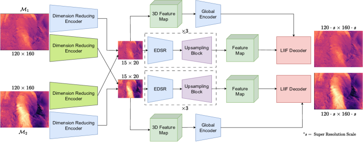
The model architecture constitutes (i) dimension reducing encoders to encode high resolution weather data into a low resolution space, (ii) feature encoders that learn the spatial features from the low resolution representations, and (iii) implicit neural network decoders that use the extracted features by the feature encoders and predicts the wind data for that specific coordinate. We worked with 2 different modalities, and . Figure 1 summarizes the proposed methodology. We define each modality as wind data at different heights from the ground. Specifically, weather data at units above from the ground is considered as modality , similarly constitutes data at units above the ground, conditioned on .
3.2.1 Dimension Reducing Encoder
Two different kinds of convolutional neural network based dimension reduction encoders, self-encoders and cross-modal encoders, with the similar architecture, encodes high resolution data to low resolution space. Self encoders convert the high resolution data from one modality to its corresponding low resolution representation, whereas the cross-modal encoders converts it into a different modality. Let and be the high resolution data space of and correspondingly. Similarly and be the low resolution data space of and correspondingly. Then, self encoders can be defined as
| (1) |
and the cross-modal encoders can be defined as
| (2) |
The architecture of the encoder is inspired from the architecture proposed in the downsampling part of the invertible UNet [18].
3.2.2 Local Implicit Image Function based Decoder
Local implicit image function (LIIF) based decoder is a coordinate based decoding approach which takes the coordinate and the deep features around that coordinate as inputs and outputs the value for that corresponding coordinate [19]. Due to the continuous nature of spatial coordinates, LIIF-based decoder can decode into arbitrary resolution.
| (3) |
Here, and are two EDSR-based [20] feature encoders for modalities and into the encoded feature space and respectively. We use , , to denote channel depth, height and width of the corresponding encoded feature space. Let be a 2-D coordinate space. We follow the feature extraction method discussed in LIIF [19]. Let the LIIF based feature extractor be
| (4) |
where is the extracted feature dimension, and extracted feature at coordinate is . Decoders are functions that take the encoded features, at specific coordinate, as input. For example,
| (5) |
are two coordinate based decoders for modalities and .
3.2.3 Global Encoding Incorporated LIIF
Global encoders are functions of the low-resolution representation. and are global encoders for modalities and , with as the dimension of the global encoding. Unlike the local implicit neural network based decoder proposed in LIIF [19], our proposed GEI-LIIF(Global Encoding Incorporated Local Implicit Image Function) based modality specific decoder, is a function of two features:
-
•
Extracted local feature at coordinate through
(6) -
•
Extracted global feature through
(7)
predicts the target value at coordinate for modality, .
3.2.4 Self & Cross Modality Prediction
Let be a data instance with high resolution in modality . With the self-encoder and cross-modal encoder we can get the low dimensional representation of this data instance in both modalities, and consequently achieve continuous super-resolution with the GEI-LIIF based decoder in both modalities, . For example, for a co-ordinate point ,
| (8) |
represents the prediction at modality or self-prediction and
| (9) |
represents the prediction at modality or cross-prediction. Similarly, for a data instance and for a co-ordinate point ,
| (10) |
represents the prediction at modality or self-prediction and
| (11) |
represents the prediction at modality or cross-prediction.
4 Results
4.1 Experimental Setup
• Data The data considered in this paper is generated from the National Renewable Energy Laboratory’s Wind Integration National Database (WIND) Toolkit. Specifically, we built the data set for multi-modal super-resolution tasks using simulated wind data. We randomly sampled data points from different timestamps among the total available instances for each height above from the ground (, , and ), with data points for training the models and data points for testing. We took wind data from two different heights from the pool of and as the two different modalities. We took two combinations: () and () for doing the experiments. We used bicubic interpolation to generate a pair of high-resolution and super-high-resolution samples for each instance. For example, if the input dimension at both modalities is , and the super-resolution scale is , then the output super-high-resolution dimension is .
• Training The loss function, combines two reconstruction terms, with a latent term,
| (12) |
The reconstruction terms enable the model to capture signals through both self-prediction and cross-prediction. The latent term promotes the learning of compact, low-dimensional representations.
| (13) |
| (14) |
| (15) |
Unlike CLUE [11], we do not enforce our model to learn a unified latent space representation which gives us the freedom to bypass the need for a modality classifier model and an adversarial loss function for optimization.
4.2 Observed Results
We tested the performance of our model at different super-resolution scales for both self and cross predictions on the test dataset consisting datapoints. The high resolution input dimension was set to and the low resolution representation had a dimension of . We used a pretrained ResNet18 [21] model as the global encoder that encodes the low dimensional representation and extracts the features as a vector, and finetuned the weights while optimizing the other parts of the model.
4.2.1 Super-Resolution Performance
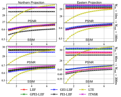
We tested the super-resolution performance of our designed GEI-LIIF decoder by replacing it with various other super-resolution models. We also made some modifications in our proposed methodology and compared the performances with these modified models. As the baseline, we chose LIIF based decoder for modality specific super-resolution where the decoder only takes the extracted local features as its input. Positional encoders are functions of the 2-D coordinates based on Fourier based positional encoding. is the positional encoder with as its input with as the dimension of the positional encoder output. We design PEI-LIIF (Positional Encoding Incorporated Local Implicit Image Function) decoder, and GPEI-LIIF (Global & Positional Encoding Incorporated Local Implicit Image Function), . PEI-LIIF uses extracted local features and positional encodings as its input, whereas GPEI-LIIF uses extracted local features, global features and positional encodings as its input. We also compared our designed decoder with local texture estimator based decoder (LTE) [22], and implicit transformer network based decoder (ITNSR) [23]. Figure 2 shows the comparative results for the cross-prediction scenarios where the input modality height is closer to the ground and the output modality height is much higher above from the ground.
4.2.2 Compression Performance
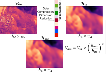
We tested our approach and compared its compression performance with other data compression methods. We used prediction by the partial matching (PPM) data compression algorithm with the -law based encoding at different quantization levels () to compress and reconstruct data [24]. We also tested bicubic interpolation to compress and decompress the data. For comparison of cross-modal predictions, we used the wind power law to transform the reconstructed data at one height to another height according to the equation, [25], with the PPM and bicubic methods. Figure 3 summarizes the cross-modal prediction performances by these methods. Table 1 shows the data compression performance for different methods. We set and for the PPM and bicubic methods. As this workflow is only capable of reconstructing the output as the same dimension of the input, we set the super-resolution scale for GEI-LIIF and GPEI-LIIF models for a fair comparison. Unlike super-resolution results, we also tested dimension reduction factor for bicubic, GEI-LIIF and GPEI-LIIF models to see how these methods perform compared to compression methods when dimension reduction factor is smaller.
| Northern Projection | |||
| Method | CR | PSNR | SSIM |
| 95.0584 | 24.1419 | 0.4104 | |
| 92.8557 | 28.3741 | 0.6147 | |
| 98.4375 | 28.6436 | 0.5506 | |
| 93.7500 | 29.4141 | 0.6157 | |
| 98.4375 | 29.2306 | 0.5996 | |
| 93.7500 | 29.6598 | 0.6407 | |
| 95.7176 | 24.2708 | 0.4699 | |
| 93.6066 | 29.2434 | 0.6793 | |
| 98.4375 | 29.8462 | 0.6144 | |
| 93.7500 | 31.0304 | 0.6917 | |
| 98.4375 | 29.4583 | 0.6342 | |
| 93.7500 | 30.7283 | 0.7049 | |
| Eastern Projection | |||
| Method | CR | PSNR | SSIM |
| 94.8006 | 23.8402 | 0.4493 | |
| 92.5589 | 28.4303 | 0.6527 | |
| 98.4375 | 28.4412 | 0.5379 | |
| 93.7500 | 29.5427 | 0.6191 | |
| 98.4375 | 29.433 | 0.5959 | |
| 93.7500 | 30.4430 | 0.6646 | |
| 95.3462 | 23.6018 | 0.5028 | |
| 93.2222 | 29.3593 | 0.7089 | |
| 98.4375 | 29.3787 | 0.5887 | |
| 93.7500 | 30.8214 | 0.6800 | |
| 98.4375 | 30.3195 | 0.6522 | |
| 93.7500 | 30.8097 | 0.6818 | |
4.3 Discussion
Figure 2 shows the super-resolution performances for different decoders for 8 different cases (2 projections, 2 different cross-modal scenarios for each projection, 2 metrics for each cross-modal scenario). Among them, GEI-LIIF comes out to be the best performing one in 4 cases, whereas ITNSR decoder does the best in the other 4 cases. At some extreme scales, LTE beats other models but performs poorly in other super-resolution scales. In terms of compression performance, our proposed model (either with GEI-LIIF or GPEI-LIIF decoder) outperforms PPM or Bicubic models in terms of compression ratio. The compression models achieve high PSNR and SSIM only when the compression ratios are the lowest. These models are not capable of achieving the best performance in all three metrics simultaneously. Due to space limitations, we do not show the model performance in other cross-modal scenarios where the input height modality is much higher above the ground and the output modality is much closer to the ground as those cases are not of greater concern compared to its counterpart, nor the self prediction cases. But the results in those cases are similar to what we see in this cross-modal scenario, both in terms of super-resolution and compression performance. In terms of super-resolution performance, GEI-LIIF is not always beating its counterparts, rather ITNSR comes out to be the champion in the same number of cases. This indicates that there should be a better way of fusing the global and local features at the decoding stage to achieve better super-resolution performance, and it still remains an open question.
5 Conclusion
We proposed a novel deep learning solution for simultaneous continuous super-resolution, data dimensionality reduction, and multi-modal learning of climatological data. We specifically developed a local implicit neural network model for learning continuous, rather than discrete, representations of climate data, such as wind velocity fields used for wind farm power modeling across the continental United States, along with multi-modal dimension reducing encoder that facilitates dimension reduction and cross modality extrapolation. We also introduced a latent loss function to ensure cross modality learning. Obtained results have shown the promising potential to solve real-world scenarios in wind energy resource assessment for electricity generation, efficient storage of huge amount of data by dimensionality reduction, and extrapolation of data to inaccessible spatial spaces (e.g., specific altitudes) from available wind data. However, our model is feasible only for a small number of modalities as the total number of encoders will increase quadratically with the increase of modalities. Designing a more scalable model that can handle a higher number of modalities is a topic for future research.
References
- [1] Christopher Irrgang et al., “Towards neural earth system modelling by integrating artificial intelligence in earth system science,” Nature Machine Intelligence, vol. 3, no. 8, pp. 667–674, 2021.
- [2] Karthik Kashinath et al., “Physics-informed machine learning: case studies for weather and climate modelling,” Philosophical Transactions of the Royal Society A, vol. 379, no. 2194, pp. 20200093, 2021.
- [3] Milan Klöwer et al., “Compressing atmospheric data into its real information content,” Nature Computational Science, vol. 1, no. 11, pp. 713–724, 2021.
- [4] Langwen Huang and Torsten Hoefler, “Compressing multidimensional weather and climate data into neural networks,” in The Eleventh International Conference on Learning Representations, 2023.
- [5] Zhihan Gao et al., “Earthformer: Exploring space-time transformers for earth system forecasting,” Advances in Neural Information Processing Systems, vol. 35, pp. 25390–25403, 2022.
- [6] Codruț-Andrei Diaconu et al., “Understanding the role of weather data for earth surface forecasting using a convlstm-based model,” in Proceedings of the IEEE/CVF Conference on Computer Vision and Pattern Recognition, 2022, pp. 1362–1371.
- [7] Tung Nguyen et al., “Climax: A foundation model for weather and climate,” arXiv preprint arXiv:2301.10343, 2023.
- [8] Christian Requena-Mesa et al., “Earthnet2021: A large-scale dataset and challenge for earth surface forecasting as a guided video prediction task.,” in Proceedings of the IEEE/CVF Conference on Computer Vision and Pattern Recognition, 2021, pp. 1132–1142.
- [9] Xihaier Luo et al., “Reinstating continuous climate patterns from small and discretized data,” in 1st Workshop on the Synergy of Scientific and Machine Learning Modeling@ ICML2023, 2023.
- [10] Xihaier Luo et al., “Continuous field reconstruction from sparse observations with implicit neural networks,” arXiv preprint arXiv:2401.11611, 2024.
- [11] Xinming Tu et al., “Cross-linked unified embedding for cross-modality representation learning,” in Advances in Neural Information Processing Systems, Alice H. Oh, Alekh Agarwal, Danielle Belgrave, and Kyunghyun Cho, Eds., 2022.
- [12] Arturo A Keller et al., “Downscaling approaches of climate change projections for watershed modeling: Review of theoretical and practical considerations,” PLoS Water, vol. 1, no. 9, pp. e0000046, 2022.
- [13] Paula Harder et al., “Hard-constrained deep learning for climate downscaling,” Journal of Machine Learning Research, vol. 24, no. 365, pp. 1–40, 2023.
- [14] Brian Groenke et al., “Climalign: Unsupervised statistical downscaling of climate variables via normalizing flows,” in Proceedings of the 10th International Conference on Climate Informatics, 2020, pp. 60–66.
- [15] Yumin Liu et al., “Climate downscaling using ynet: A deep convolutional network with skip connections and fusion,” in Proceedings of the 26th ACM SIGKDD International Conference on Knowledge Discovery & Data Mining, 2020, pp. 3145–3153.
- [16] Yiheng Xie et al., “Neural fields in visual computing and beyond,” Computer Graphics Forum, vol. 41, no. 2, pp. 641–676, 2022.
- [17] Jonathan Richard Schwarz et al., “Modality-agnostic variational compression of implicit neural representations,” arXiv preprint arXiv:2301.09479, 2023.
- [18] Christian Etmann et al., “iunets: learnable invertible up-and downsampling for large-scale inverse problems,” in 2020 IEEE 30th International Workshop on Machine Learning for Signal Processing (MLSP). IEEE, 2020, pp. 1–6.
- [19] Yinbo Chen et al., “Learning continuous image representation with local implicit image function,” in Proceedings of the IEEE/CVF Conference on Computer Vision and Pattern Recognition, 2021, pp. 8628–8638.
- [20] Bee Lim et al., “Enhanced deep residual networks for single image super-resolution,” in The IEEE Conference on Computer Vision and Pattern Recognition (CVPR) Workshops, July 2017.
- [21] Kaiming He et al., “Deep residual learning for image recognition,” in Proceedings of the IEEE Conference on Computer Vision and Pattern Recognition (CVPR), June 2016.
- [22] Jaewon Lee et al., “Local texture estimator for implicit representation function,” in Proceedings of the IEEE/CVF Conference on Computer Vision and Pattern Recognition (CVPR), June 2022, pp. 1929–1938.
- [23] Jingyu Yang et al., “Implicit transformer network for screen content image continuous super-resolution,” in Advances in Neural Information Processing Systems, A. Beygelzimer, Y. Dauphin, P. Liang, and J. Wortman Vaughan, Eds., 2021.
- [24] A. Moffat, “Implementing the ppm data compression scheme,” IEEE Transactions on Communications, vol. 38, no. 11, pp. 1917–1921, 1990.
- [25] Jawad S. Touma, “Dependence of the wind profile power law on stability for various locations,” Journal of the Air Pollution Control Association, vol. 27, no. 9, pp. 863–866, 1977.