Self-organization and memory in an amorphous solid subject to random loading
Abstract
We consider self-organization and memory formation of a sheared amorphous solid subject to a random shear strain protocol confined to a strain range . We show that, as in the case of applied cyclic shear, the response of the driven system retains a memory of the strain range that can subsequently be retrieved. Our findings suggest that self-organization and memory formation of disordered materials can emerge under more general conditions, such as a system interacting with its fluctuating environment.
Consider two pairs of identical shoes: one has been worn by you over an extended period, while the other has never been worn and is therefore kept in pristine condition. An example is shown in Fig. 1(a). The one that has been broken-in will reflect features of you: your gait and, more generally, aspects of your lifestyle, perhaps an active one where you frequently run or jump or a more leisurely one where you walk. Next, consider a friend who has the same shoe size as you and imagine what would happen if you invited him/her to wear your worn pair. To your friend, the shoes will probably not feel right at first and will require being broken-in once again. As wearers of the shoes, each of you subjects them to mechanical deformations that are unique to you. As a result, the way you wear the shoes leaves an imprint – or memory – on them. Having someone else wear your own shoes will eventually cause some loss of this memory.
Likewise, disordered materials exhibit a memory of their mechanical past. In experiments on athermal disordered systems driven by oscillatory deformations, such as colloidal suspensions Keim and Nagel (2011); Paulsen et al. (2014); Keim and Arratia (2014); Keim et al. (2020) or crumpled thin elastic sheets Shohat et al. (2022); Mungan (2022), it is found that after several driving cycles, such systems self-organize into a periodic response that retains a memory of the deformation amplitude, which can subsequently be read-out Keim et al. (2019); Paulsen and Keim (2024). Self-organization and memory formation under cyclic shear has also been observed in numerical simulations of atomistic as well as mesoscopic models of sheared amorphous solids Fiocco et al. (2014); Regev et al. (2015); Priezjev (2016); Yeh et al. (2020); Bhaumik et al. (2021); Liu et al. (2022); Khirallah et al. (2021); Kumar et al. (2022, 2024).
How can one retrieve the amplitude of past oscillatory driving? An experimentally realizable read-out protocol consists of subjecting the “trained” system to single cycles of oscillatory deformations, with the amplitude after each driving cycle being incremented by a fixed amount. By comparing the configuration state of the system prior to the read-out with the ones obtained at the end of each driving cycle, it is found that the discrepancy between these two is minimal when read-out and training amplitude match. Moreover, this discrepancy rises sharply once the read-out amplitude exceeds the training amplitude Keim et al. (2019); Paulsen and Keim (2024).
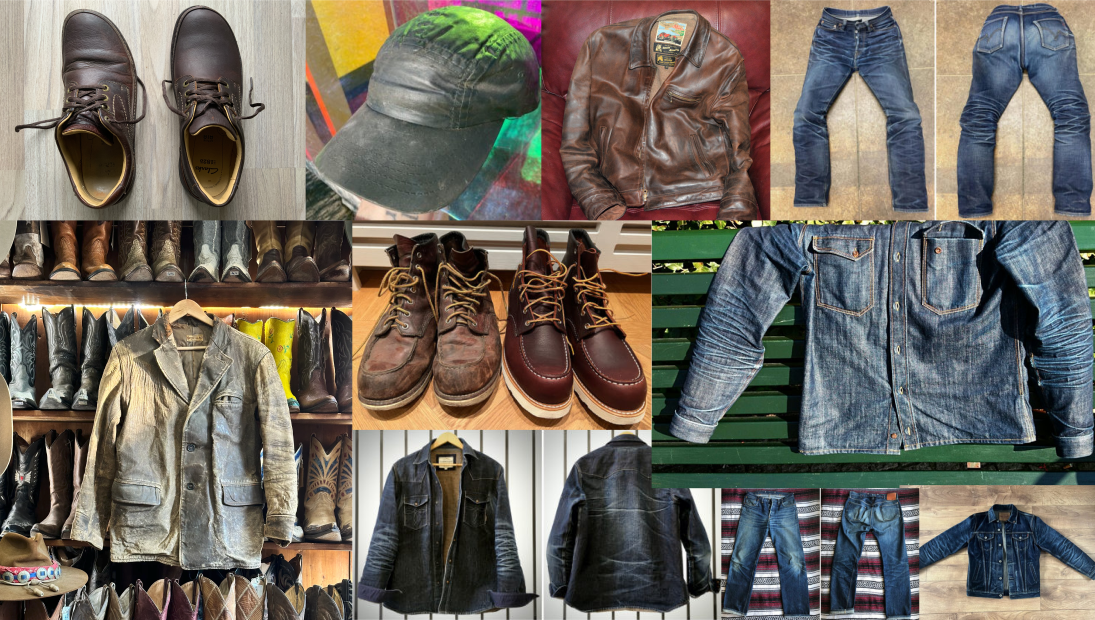
The example of the broken-in shoe, and more generally of worn clothes as illustrated in Fig. 5, suggests that the mechanical deformation does not have to be strictly oscillatory for a memory of the driving to be imprinted on it. Here, we present simulations of a 2d elastoplastic model of an amorphous solid subject to a random shear strain protocol and show that such driving can also cause the solid to self-organize into a state that retains memory, similar to the case of driving by oscillatory shear.
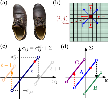
Elastoplastic Model of a Sheared Amorphous Solid – We consider the 2d Quenched Mesoscopic Elasto Plastic (QMEP) model of an amorphous solid introduced in Refs. Kumar et al. (2022, 2024), and which qualitatively reproduces the response of sheared amorphous solids to oscillatory shear. The sample is coarse-grained into mesoscale blocks, each of which can yield and redistribute local stresses in response to an applied shear strain Nicolas et al. (2018). In particular, we associate a stack of local elastic branches with each mesoscale block, labeled by an integer , as illustrated in Fig. 1 (b) and (c). Under athermal quasistatic (AQS) loading, the internal stress and strain of each block follow their branch segment until its termination at or , depending on the shearing direction. At this point, the mesoscopic block yields, and a transition to one of the corresponding neighbouring branches occurs. During the local yield event, the internal stresses are redistributed among the other blocks. The stress redistribution follows a quadrupolar pattern, mimicking the effect of an Eshelby inclusion on the surrounding elastic matrix Eshelby (1957). Note that each elastic branch is assigned a given pair of thresholds , hence the quenched character of the disorder: the same thresholds can be visited several times in a back and forth motion (refer to Kumar et al. (2022) for details on the elastic interaction and the threshold disorder).
At the macroscopic scale, the stress response to an externally applied strain consists of a sequence of global elastic branches punctuated by stress drops. Each elastic branch has a stability range which is determined by the local branch configurations with the requirement that under elastic deformations, each cell , experiencing the local stress , remains on its local branch Kumar et al. (2022). We will call these global elastic branches mesostates and label them in capital letters. In Fig. 1(d), we illustrate the transitions out of the elastic branch to branches and upon the increase, respectively decrease, of the applied shear strain.
Random Driving Protocol – While loading by simple cyclic shear cycles is unambiguously defined, a wide variety of random loading protocols can be considered. Here, we consider a simple random walk along the strain axis with reflective boundaries at shear strains . Starting at the origin , our random driving consists of taking finite strain steps of size with , so that it takes at least steps for the walker to reach one of the reflecting boundaries from the origin. In the following, we deal with strain steps of magnitude larger than the typical stability range of mesostates. In the case the walker lands in a mesostate whose stability range is larger than the strain step, i.e. when , we first choose randomly a direction and then apply a strain in that direction, with such that the resulting strain is closest yet outside the corresponding end of the elastic branch, as illustrated in Fig. 2(a). This implementation minimizes the time the walker spends on elastic branches and ensures the symmetry of the random walk since, by design, it is equally likely to leave the elastic branch from either end. Let us emphasize that our primary goal is to demonstrate memory formation under driving conditions as unbiased and random as possible.
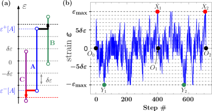
In analogy with driving by cyclic shear, we next define a cycle for our random driving protocol. The system starts in a freshly prepared glass at zero applied strain and is then subject to a random walk along the strain axis, as described. Fig. 2(b) shows a typical deformation path. In this example, the boundary is hit first. We, therefore, define the direction of negative strain as the forward shearing direction and label the corresponding mesostate when this boundary is hit as . We next track the first time the system reaches the opposite boundary after and label the corresponding mesostate . The first cycle completes with the first return to zero strain at mesostate , as indicated in Fig. 2(b). Next, the mesostate corresponds to the first time the system hits the forward boundary again after reaching , etc. Our training protocol consists of applying random cycles to a fresh glass . 111Note that the forward passages or require far more steps than the reverse ones, i.e. and . This is a direct consequence of the Bauschinger effect Patinet-Bauschinger-PRL20.
Simulation Details – We generated poorly annealed (PA) glasses of size mesoscale blocks and subjected them to random driving. Details of the sample preparation protocol can be found in Kumar et al. (2022), where it was shown that for PA samples, a cyclic response can be obtained with high probability up to a strain amplitude of Kumar et al. (2022). This value marks the onset of the irreversibility transition Pine et al. (2005); Corte et al. (2008); Keim and Nagel (2011); Denisov et al. (2015); Lavrentovich et al. (2017); Yeh et al. (2020); Bhaumik et al. (2021); Sastry (2021); Mungan and Sastry (2021); Parley et al. (2022); Kumar et al. (2022); Reichhardt et al. (2023).
We considered random driving protocols with maximum strain values of and , using random walk step sizes of , , and . We drove the system for a maximum number of random cycles. As we describe next, we find that memory features already establish themselves after about 10 driving cycles. In addition, our results on memory encoding and retrieval turn out to be qualitatively similar for all the strain ranges and step sizes we considered. In the following, we therefore show only results for glasses driven for cycles with and . The appendix contains results for the other strain ranges.
Read-out Protocols – Having trained our system for a given number of driving cycles, we denote the mesostate reached at the end of the driving as the trained state . We perform a read-out protocol on by applying a single cycle of simple oscillatory shear at a read-out amplitude , i.e. , with depending on whether at the beginning of read-out we increase or decrease the strain first.
Suppose that at this stage, we have the knowledge of the sense of the driving established during training, i.e. we know whether the or boundary was reached first. We can have a read-out that is in-phase with the sense of training Kumar et al. (2024), which we will call the forward (FWD) read-out, where the direction in which the read-out strain initially changes is towards the boundary hit first. Conversely, if the direction of read-out strain initially points opposite to it, and hence it is out-of-phase with the training, this will be referred to as a reverse (REV) read-out. For the example shown in Fig. 2(b), where the boundary was reached first, correspond to a FWD read-out protocol, while is a REV read-out. Regardless of the sense of direction, we will denote the state reached at the end of the first read-out cycle as .
Next, we define a distance between the two mesostates and by comparing their corresponding sets of local branch indices and as follows:
| (1) |
i.e. we count the number of mesoscale blocks for which the local branch numbers are different and divide by the total number of blocks.
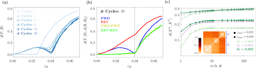
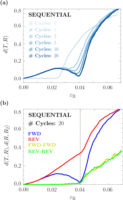
Memory after Random Driving – Fig 3(a) shows the behavior of with FWD read-out at various amplitudes and for different numbers of driving cycles for glasses trained at . The data points are averaged over realizations, and we consider a parallel read-out protocol: for each glass, we keep a copy of and then apply the read-outs at different amplitudes to the same . An experimentally realizable sequential read-out protocol leads to similar results and is presented in the appendix, Fig. A2.
As a control, we also performed a read-out on the freshly prepared glasses , i.e. a state without prior shear. The distance remains zero up to a read-out strain of . This value is consistent with the typical stability range of the trained state, indicating that over this range of read-outs our glass will likely respond purely elastically and return to the initial configuration after one read-out cycle. The remaining graphs in Fig 3(a) show the results of read-outs after and random driving cycles. Already for , a local minimum of appears near the training amplitude . With increasing , this dip becomes cusp-like and moves towards . Note that the corresponding curves are nearly indistinguishable for and . We have verified that this behavior does not change when the random driving is further increased up to cycles.
We performed the read-out in the FWD direction to recover the training amplitude . As mentioned earlier, this requires knowing which of the two reflecting boundaries was hit first during training. We next ask how behaves if we use the reverse read-out protocol REV instead. This is shown in Fig 3(b), where we compare the results of the FWD (blue) and REV (red) read-out protocols applied to . We see that the REV protocol is not able to detect 222In the case of simple oscillatory shear and for training amplitudes well below the irreversibility transition, a memory of the shear amplitude can be detected in REV read-outs, as revealed by a sudden increase of the slope of Kumar et al. (2024). Similarly, in Fig. A3(a) for and , a kink of at is clearly discernible, but gets fainter with increasing .. This finding is consistent with our recent work on memory formation in the QMEP model under simple oscillatory shear Kumar et al. (2024).
RPM-based Read-out Protocols – A read-out protocol that can detect without a knowledge of the FWD sense of driving could be defined if the response of the amorphous solid were to possess the return-point memory (RPM) property. RPM is the property of a system to be able to return to a state at which the direction of driving has been reverted and leads to a nested hierarchy of hysteresis cycles Sethna et al. (1993); Mungan and Terzi (2019); Terzi and Mungan (2020). It is a property of magnets with ferromagnetic spin interactions and elastic manifolds driven through random disorder Middleton (1992), where the stress distribution upon triggering an instability is systematically destabilizing. Owing to the anisotropic nature of stress distribution in sheared amorphous solids, localized yielding events can destabilize and destabilize other parts of the sample. Hence, RPM is not expected to hold a priori in such systems. Nevertheless, recent work on driven disordered systems has demonstrated experimentally as well as numerically that these systems can exhibit near-perfect RPM Keim et al. (2020); Mungan et al. (2019); Shohat et al. (2022); Shohat and Lahini (2023).
We, therefore, define a read-out protocol that is sensitive to RPM. Denote by the mesostate reached when applying to an additional read-out cycle at the same amplitude and sense of direction. If RPM were to hold then Middleton (1992); Sethna et al. (1993); Mungan and Terzi (2019) (see also 333More precisely, over a range of driving amplitudes. In the case of ferromagnets, one would not expect a bound on the applied field due to the possibility of magnetization saturation. However, in the case of a driven elastic manifold, this range would be limited by the onset of depinning, beyond which quasi-static configurations are not attainable anymore.). Thus, instead of considering , we observe the behavior of with read-out amplitude. Depending on the sense chosen, we will refer to these as the FWD-FWD and REV-REV read-out protocols. The ocher (green) curve in Fig 3(b) shows the read-outs under the FWD-FWD (REV-REV) protocols. Note that both protocols are insensitive to the driving direction and exhibit near indistinguishable behavior of with . Moreover, up to the training amplitude , after which it rises sharply. Thus, when restricted to , we find that the trained glasses exhibit a response highly reminiscent of RPM. In the absence of any information on the training direction, the application of this RPM-inspired reading protocol allows us to retrieve the maximum amplitude of the material’s past random driving.
Ensemble of Trained States and Self-Organization – For each glass , applying simple oscillatory shear cycles of fixed amplitude leads to a unique trained state . This is, of course, not the case for random driving: given a glass and , each random driving protocol will mechanically anneal the glass differently and, therefore, lead to a different trained state. The random driving provides us with an ensemble of trained glasses that all originated from the common glass , equivalent to an isoconfigurational ensemble Widmer-Cooper et al. (2004) employed in supercooled liquids to quantify what part of the dynamics can be ascribed to the structure. We next characterize its properties.
We considered a single poorly-aged glass and formed ensembles of and random training protocols that were applied to with and , respectively. We track the evolution over cycles, and in each cycle , we record for each member the configurations at position , cf. Fig. 2(b).
First, we split the ensemble according to whether its members hit or first. For the sake of simplicity, we only consider the larger of the two groups and calculate the pair-distances among its members, using (1). The main panel of Fig. 3(c) shows the evolution of the ensemble-averaged pair-distance with cycle number for different random walk step-sizes , as indicated in the legend. Irrespective of training amplitude and step size, the pair distance approaches saturation rather quickly. This approach becomes somewhat slower with decreasing . Nevertheless, the ensemble of trained configurations appears to be asymptotically equidistant.
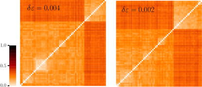
The inset of Fig. 3(c) shows a hierarchical clustering of the members of the ensemble trained at and using (color coding of distance as indicated by color bar). The clustering was based on the pair-distances at cycle 20, which can be regarded as an overlap Jaiswal et al. (2016). We see that the trained glasses break into two large clusters and , as indicated. Not surprisingly, this grouping turns out to be according to the boundary they hit first. However, within each of these two clusters, there is visible sub clustering, indicating the presence of clusters of trained glasses that are closer to each other than the rest. Strikingly, subclustering becomes less pronounced with decreasing , as shown in Fig. A4.
Discussion – Our findings show that memory formation and retrieval in amorphous solids can be achieved under random driving. It is qualitatively very similar to its counterpart of applying simple oscillatory shear, as was studied recently in Kumar et al. (2024). Thus it is not the driving protocol itself but the range of applied strains, as captured by , that encodes the memory. A natural setting of random driving is that of a system interacting with its fluctuating environment, and our results imply that the latter can leave an imprint on the former.
The random driving protocol leads to a self-organization of the response of the amorphous solid. In the spirit of the limit cycles obtained under simple oscillatory driving, we can think of this self-organization as leading to a collection of mesostates that can be repeatedly revisited under the various read-out protocols. This collection of states is marginally stable in the sense that the self-organization results in the accessibility of these states only if the time-dependent driving protocol is confined to stay below the training amplitude, i.e. . This is most clearly seen from the RPM-like behavior observed under the FWD-FWD or REV-REV read-outs persisting up to read-out amplitudes , cf. Fig. 3(b), as well as Figs. A2(b) and A3(b) in the appendix.
More generally, we may ask for the nature of the self-organization that emerges under the random driving protocol. In particular, the possibility of dynamical attractors into which the driving may lead and trap the system, as well as the questions of reversibility underlying the memory formation are most conveniently addressed within the perspective of the transition graph (-graph) description of the response of driven systems under general AQS driving protocolsMungan et al. (2019); Regev et al. (2021); Kumar et al. (2022). A discussion of our results from this perspective is given in the Appendix.
We considered a simple random walk with finite strain steps and reflecting boundaries at well-defined strains . The nature of the real fluctuations experienced by materials in working conditions is obviously far more complex. A natural perspective of this work would consist of relaxing the boundary condition and testing the effect of spatial and temporal correlations in random driving or testing the effect of thermal noise in the broader context of aging. In the present case, energy is injected at a large scale. In a complementary view, active matter can be seen as random driving operating at a small scale Agoritsas and Morse (2024); Goswami et al. (2023); Alert et al. (2022). It would be instructive to compare the self-adaptation process and the memory behavior obtained in these contrasting conditions. It would also be of interest to probe the adaptive response of active biological tissues to random mechanical actuation, building, for example, on work in Laplaud et al. (2021). Other natural perspectives of this work deal with the learning of disordered networks Stern et al. (2024) and the fatigue behavior of engineering materials under service Morrow (1965).
The daily life example of worn shoes naturally motivates experimental testing of mechanical memory due to random driving. The RPM-inspired sequential read-out protocol proposed here should immediately apply to driven colloidal suspensions or crumpled sheets. Keeping with the theme of breaking-in shoes, it would also be of obvious interest to test these ideas on fabric materials, e.g. the fading of jeans by natural (or artificial) wear.
Acknowledgements.
The authors would like to thank Srikanth Sastry, Yoav Lahini, Dor Shohat and Elisabeth Agoritsas for useful discussions. MM also acknowledges PMMH and ESPCI for their kind hospitality during multiple stays, which were made possible by Chaire Joliot grants awarded to him. MM was supported by the Deutsche Forschungsgemeinschaft (DFG, German Research Foundation) under Projektnummer 398962893. This project has received funding from the European Union’s Horizon 2020 research and innovation programme under the Marie Sklodowska-Curie grant agreement No. 754387.References
- Keim and Nagel (2011) N. C. Keim and S. R. Nagel, Phys. Rev. Lett. 107, 010603 (2011).
- Paulsen et al. (2014) J. D. Paulsen, N. C. Keim, and S. R. Nagel, Phys. Rev. Lett 113, 068301 (2014).
- Keim and Arratia (2014) N. C. Keim and P. E. Arratia, Phys. Rev. Lett. 112, 028302 (2014).
- Keim et al. (2020) N. C. Keim, J. Hass, B. Kroger, and D. Wieker, Phys. Rev. Res. 2, 012004 (2020).
- Shohat et al. (2022) D. Shohat, D. Hexner, and Y. Lahini, Proc. Nat. Acad. of Sci. 119, e2200028119 (2022), https://www.pnas.org/doi/pdf/10.1073/pnas.2200028119 .
- Mungan (2022) M. Mungan, Proc. Nat. Acad. Sci. 119, e2208743119 (2022).
- Keim et al. (2019) N. C. Keim, J. D. Paulsen, Z. Zeravcic, S. Sastry, and S. R. Nagel, Rev. Mod. Phys. 91, 035002 (2019).
- Paulsen and Keim (2024) J. D. Paulsen and N. C. Keim, arXiv preprint arXiv:2405.08158 (2024).
- Fiocco et al. (2014) D. Fiocco, G. Foffi, and S. Sastry, Phys. Rev. Lett. 112, 025702 (2014).
- Regev et al. (2015) I. Regev, J. Weber, C. Reichhardt, K. A. Dahmen, and T. Lookman, Nat. Commun. 6, 8805 (2015).
- Priezjev (2016) N. V. Priezjev, Phys. Rev. E 93, 013001 (2016).
- Yeh et al. (2020) W.-T. Yeh, M. Ozawa, K. Miyazaki, T. Kawasaki, and L. Berthier, Phys. Rev. Lett. 124, 225502 (2020).
- Bhaumik et al. (2021) H. Bhaumik, G. Foffi, and S. Sastry, P. Natl Acad. Sci. 118, e2100227118 (2021).
- Liu et al. (2022) C. Liu, E. E. Ferrero, E. A. Jagla, K. Martens, A. Rosso, and L. Talon, J. Chem. Phys. 156, 104902 (2022).
- Khirallah et al. (2021) K. Khirallah, B. Tyukodi, D. Vandembroucq, and C. E. Maloney, Phys. Rev. Lett. 126, 218005 (2021).
- Kumar et al. (2022) D. Kumar, S. Patinet, C. E. Maloney, I. Regev, D. Vandembroucq, and M. Mungan, J. Chem. Phys. 157, 174504 (2022).
- Kumar et al. (2024) D. Kumar, M. Mungan, S. Patinet, M. M. Terzi, and D. Vandembroucq, arXiv:2409.07621 (2024), 10.48550/arXiv.2409.07621.
- Nicolas et al. (2018) A. Nicolas, E. E. Ferrero, K. Martens, and J.-L. Barrat, Rev. Mod. Phys. 90, 045006 (2018).
- Eshelby (1957) J. D. Eshelby, Proc. R. Soc. Lond. A 241, 376 (1957).
- Note (1) Note that the forward passages or require far more steps than the reverse ones, i.e. and . This is a direct consequence of the Bauschinger effect Patinet-Bauschinger-PRL20.
- Pine et al. (2005) D. J. Pine, J. P. Gollub, J. Brady, and A. M. Leshansky, Nature 438, 997 (2005).
- Corte et al. (2008) L. Corte, P. M. Chaikin, J. P. Gollub, and D. J. Pine, Nature Physics 4, 420 (2008).
- Denisov et al. (2015) D. V. Denisov, M. T. Dang, B. Struth, A. Zaccone, G. H. Wegdam, and P. Schall, Sci. Rep. 5, 14359 (2015).
- Lavrentovich et al. (2017) M. O. Lavrentovich, A. J. Liu, and S. R. Nagel, Phys. Rev. E 96, 020101 (2017).
- Sastry (2021) S. Sastry, Phys. Rev. Lett. 126, 255501 (2021).
- Mungan and Sastry (2021) M. Mungan and S. Sastry, Phys. Rev. Lett. 127, 248002 (2021).
- Parley et al. (2022) J. T. Parley, S. Sastry, and P. Sollich, Phys. Rev. Lett. 128, 198001 (2022).
- Reichhardt et al. (2023) C. Reichhardt, I. Regev, K. Dahmen, S. Okuma, and C. J. O. Reichhardt, Phys. Rev. Res. 5, 021001 (2023).
- Note (2) In the case of simple oscillatory shear and for training amplitudes well below the irreversibility transition, a memory of the shear amplitude can be detected in REV read-outs, as revealed by a sudden increase of the slope of Kumar et al. (2024). Similarly, in Fig. A3(a) for and , a kink of at is clearly discernible, but gets fainter with increasing .
- Sethna et al. (1993) J. P. Sethna, K. Dahmen, S. Kartha, J. A. Krumhansl, B. W. Roberts, and J. D. Shore, Phys. Rev. Lett. 70, 3347 (1993).
- Mungan and Terzi (2019) M. Mungan and M. M. Terzi, Ann. Henri Poincaré 20, 2819 (2019).
- Terzi and Mungan (2020) M. M. Terzi and M. Mungan, Phys. Rev. E 102, 012122 (2020).
- Middleton (1992) A. A. Middleton, Phys. Rev. Lett. 68, 670 (1992).
- Mungan et al. (2019) M. Mungan, S. Sastry, K. Dahmen, and I. Regev, Phys. Rev. Lett. 123, 178002 (2019).
- Shohat and Lahini (2023) D. Shohat and Y. Lahini, Phys. Rev. Lett. 130, 048202 (2023).
- Note (3) More precisely, over a range of driving amplitudes. In the case of ferromagnets, one would not expect a bound on the applied field due to the possibility of magnetization saturation. However, in the case of a driven elastic manifold, this range would be limited by the onset of depinning, beyond which quasi-static configurations are not attainable anymore.
- Widmer-Cooper et al. (2004) A. Widmer-Cooper, P. Harrowell, and H. Fynewever, Phys. Rev. Lett. 93, 135701 (2004).
- Jaiswal et al. (2016) P. K. Jaiswal, I. Procaccia, C. Rainone, and M. Singh, Phys. Rev. Lett. 116, 085501 (2016).
- Regev et al. (2021) I. Regev, I. Attia, K. Dahmen, S. Sastry, and M. Mungan, Phys. Rev. E 103, 062614 (2021).
- Agoritsas and Morse (2024) E. Agoritsas and P. K. Morse, arXiv preprint arXiv:2403.11701 (2024).
- Goswami et al. (2023) Y. Goswami, G. Shivashankar, and S. Sastry, arXiv preprint arXiv:2312.01459 (2023).
- Alert et al. (2022) R. Alert, J. Casademunt, and J.-F. Joanny, Annual Review of Condensed Matter Physics 13, 143 (2022).
- Laplaud et al. (2021) V. Laplaud, N. Levernier, J. Pineau, M. S. Roman, L. Barbier, P. J. Sáez, A.-M. Lennon-Duménil, P. Vargas, K. Kruse, O. Du Roure, M. Piel, and J. Heuvingh, Sci. Adv. 7, eabe3640 (2021).
- Stern et al. (2024) M. Stern, A. J. Liu, and V. Balasubramanian, Phys. Rev. E 109, 024311 (2024).
- Morrow (1965) J. Morrow, ASTM Spec. Techn. 378, 45 (1965).
Appendix
Breaking-in of clothing
Random driving with sequential read-outs
The read-out protocols defined in the main text are parallel: it is assumed that we can retrieve the trained state for each read-out amplitude. Experimentally, this is not easy to achieve. An alternative is to perform sequential read-outs. We start with the trained state and consider a sequence of increasing read-out amplitudes . Specifically, we start our read-out with applied to : we apply two cycles of cyclic shear and record the configurations and at the end of the first and second read-out cycle. We then increase the read-out amplitude to and apply the two-cycle read-out to and continue in this manner through our list of amplitudes. As shown in Fig. A2(a) and (b), this type of read-out gives qualitatively similar results as the parallel case that was shown in Fig. 3 (a) and (b).
Parallel read-outs at different
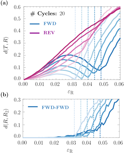
Keeping the step size at , we subjected the poorly-aged glasses to random driving protocols confined by the following maximal strains: and . Fig. A3(a) and (b) show the results of performing parallel read-outs of type FWD, REV and FWD-FWD. Shades of darker colors denote larger values of . Vertical dashed lines indicate the latter.
The FWD read-outs in panel (a) show a local minimum of the read-out distance at read-out amplitudes close to the maximum strain of the random driving. With increasing , the distance at the local minimum starts to depart from a value close to zero. The distances of the REV protocol increase monotonically with , however for , they show a discernible kink at .
Panel (b) of Fig. A3 shows the evolution of under the FWD-FWD read-out protocol. For maximum strain values up to , the distances remain small and close to zero. This behavior continues up to , beyond which starts to increase abruptly, giving rise to a kink in the read-out curves. The REV-REV read-outs show statistically similar behavior.
Attractors of the random driving protocols and the -graph representation of AQS driven systems.
We provide additional remarks on the nature of the self-organization that emerges under the random driving protocol, the possibility of dynamical attractors into which the driving may lead and trap the system, and the plastic reversibility underlying the observed formation of memory. In order to elucidate these questions, it is helpful to recall the perspective of the transition graph (-graph) description of the response of driven systems under general AQS driving protocols. Referring to Fig. 2(a) of the main text, each mesostate corresponds to an elastic branch with an upper and lower stability limit , out of which it transits into some elastic branches and . This relation can be captured by a directed graph whose vertices are the mesostates and out of which there are two transitions, leading to some other mesostates, and which we denote as the up- and down-transition and , respectively. Such -graphs can be sampled numerically, starting from the mesostate of a glass, as described in Mungan et al. (2019); Regev et al. (2021); Kumar et al. (2022). Any deformation protocol applied to thus corresponds to a specific directed path on the -graph. In this way, the dynamics of the driven system is encoded in the -graph topology.
The notion of mutual reachability decomposes such graphs into their strongly connected components (SCCs). A pair of mesostates and is mutually reachable if deformation paths exist from to as well as from to . Mutual-reachability is an equivalence relation and hence partitions the graph’s vertices into disjoint equivalence classes, namely the SCCs. Any reversible response – under oscillatory or arbitrary driving protocols – must be confined to a single SCC. Hence, the sizes of the SCCs limit the driving protocols that they can confine Regev et al. (2021).
The random driving protocol that we implemented corresponds to some unbiased random walk on the -graph. Let us consider the case where we take individual - or -steps in a random yet unbiased way and call this the -graph random walk (-RW) limited by , i.e. we do not perform - or -transitions that would require the application of a strain whose magnitude is larger than . The attractors of -RWs – if they exist – are, therefore, SCCs that can be exited only by applying strains whose magnitude exceeds . Thus, once the system is driven into such an SCC, it will be trapped there.
The random walk we implemented in the main text is different from the -RW walk described above since we restrict the applicable strains to a set of discrete values while also requiring that , cf. Fig. 2(b). Due to this restriction, these random walks will sample a subset of the mesostates that -RWs can sample, and we will call these -RWs. We can think of the graphs sampled by -RWs as coarse-grained versions of their underlying -graphs. Consequently, the trapping attractors of -RWs have lesser restrictions, as it suffices that they cannot be exited via strains that are multiples of .
Note that as , the -RWs become -RWs. Moreover, the case of simple cyclic shear corresponds to -RWs where , so that we drive the system monotonously from one boundary to the other and the driving has become deterministic.
Thus, It is interesting to study the absorption capabilities of SCCs sampled by the various random walk protocols. Size distributions of SCCs sampled from -graphs have been extracted for the QMEP model as well as from atomistic simulations Regev et al. (2021); Kumar et al. (2022) and are found to be rather broad, exhibiting power-law behavior Regev et al. (2021); Kumar et al. (2022). It was observed in Regev et al. (2021); Kumar et al. (2022) that with increasing , SCCs that can trap cyclic shear at that driving amplitudes become increasingly rare. At the same time, it was found that many of the SCCs trapping cyclic shear at an amplitude also happened to trap -RWs at this amplitude, meaning that an escape from SCCs could only happen by applying strain magnitudes larger than . These findings thus provide numerical evidence for -RW trapping SCCs. Moreover, given a limiting strain , an SCC that traps a -RW necessarily will also trap -RW. Thus, one would expect that -RW trapping SCCs might be more prevalent but will become rare as is decreased.
Lastly, in Regev et al. (2021); Kumar et al. (2022), it was observed that trapping SCCs reached under simple oscillatory shear, even if not being trapping -RWs, nevertheless have typically few escape routes compared to the number of states these SCC confine. Such transitions out of SCCs are, by definition, irreversible and have been called rabbit holes in Mungan et al. (2019). These “leaky” SCCs might nevertheless play a role in the transient dynamics towards trapping SCCs. The relatively few out of such SCCs could have a focusing or canalizing effect on the dynamics. Once such SCCs are entered, many driving trajectories within them will eventually leave from a few exits. The clustering of independent -RW see in the inset of Fig. 3(c) of the main text and Fig. A4 may be indicative of such a process. This type of canalizing might even be part of a process in which the SCCs that are entered and left are similar but whose leaky exits are successively plugged.