Humps on the profiles of the radial-velocity distribution and the age of the Galactic bar
Abstract
We studied the model of the Galaxy with a bar which reproduces well the distributions of the observed radial, , and azimuthal, , velocities derived from the Gaia DR3 data along the Galactocentric distance . The model profiles of the distributions of the velocity demonstrate a periodic increase and the formation of a hump (elevation) in the distance range of 6–7 kpc. The average amplitude and period of variations in the velocity are km s-1 and Gyr. We calculated angles , and which determine orientations of orbits relative to the major axis of the bar at the time intervals: 0–1, 1–2 and 2–3 Gyr from the start of simulation. Stars whose orbits change orientations as follows: , and , make a significant contribution to the hump formation. The fraction of orbits trapped into libration among orbits lying both inside and outside the Outer Lindblad Resonance (OLR) is 28%. The median period of long-term variations in the angular momentum and total energy of stars increases as Jacobi energy approaches the values typical for the OLR but then sharply drops. The distribution of model stars over the period has two maxima located at and Gyr. Stars with orbits lying both inside and outside the corotation radius (CR) concentrate to the first maximum. The distribution of stars whose orbits lie both inside and outside the OLR depends on their orientation: orbits elongated perpendicular to the bar concentrate to the first maximum but those stretched parallel to the bar concentrate to the second maximum. The fact that the observed profile of the -velocity distribution derived from the Gaia DR3 data does not show a hump suggests that the age of the Galactic bar, counted from the moment of reaching its full power, must lie near one of two values: or Gyr.
keywords:
Galaxy: kinematics and dynamics, galaxies with bars, Gaia DR320245081[21]
September 2, 2024; in final form, September 12, 2024
1 1. Introduction
Infrared observations provide irrefutable evidence that the Galaxy includes a bar. The position angle of the bar relative to the Sun amounts to (Dwek et al., 1995; Benjamin et al., 2005; Cabrera-Lavers et al., 2007; González-Fernández et al., 2012; Ness & Lang, 2016). Estimates of the angular velocity of the bar rotation, , obtained, among other things, from kinematical data, give a value of in the range of 40–60 km s-1 kpc-1 (Kalnajs, 1991; Dehnen, 2000; Minchev et al., 2007; Gerhard, 2011; Antoja et al., 2014; Monari et al., 2017; Melnik, 2019; Melnik et al., 2021; Asano et al., 2022, and other papers).
The positions of the resonances of the bar in the Galactic disk are determined from the following condition:
| (1) |
where is the number of full epicyclic oscillations that a star makes during revolutions relative to the bar. The ratio corresponds to the position of the Inner Lindblad Resonance (ILR) and the ratio determines the radius of the Outer Lindblad Resonance (OLR). The ultraharmonic resonances 4/1 are also important (Contopoulos, 1983; Contopoulos & Grosbol, 1989; Athanassoula, 1992).
Estimates of the age of the Galactic bar differ significantly. Cole & Weinberg (2002) studied the distribution of carbon stars in the Galaxy and estimated the age of the Galactic bar to be less than 3 Gyr. The studies of stellar ages in the Galactic bulge showed the presence of a noticeable fraction of stars of intermediate ages (2–5 Gyr) (Nataf, 2016; Bensby et al., 2017; Hasselquist et al., 2020, and other papers). The resent episodes of star formation in the bar region can be triggered by the formation of a strong bar. Nepal et al. (2024) studied a sample of super-metal-rich stars in the solar neighborhood and found a sharp change in the age-metallicity relation Gyr ago which can indicate the end of the bar formation era. Bovy et al. (2019) estimated the age of the Galactic bar to be Gyr. Debattista et al. (2019) modelled the X-shape for stars of varying ages and found the age of the Galactic bar to be greater than 5 Gyr. Sanders et al. (2024) studied Mira variables in the nuclear stellar disk and obtained the age of the Galactic bar to be greater than 8 Gyr.
Many galaxies with a bar include outer elliptical resonance rings forming near the OLR of the bar. There are two types of the outer rings: rings elongated perpendicular to the bar and rings elongated parallel to the bar. The outer ring lies a bit closer to the galactic center than the ring (Schwarz, 1981; Buta & Crocker, 1991; Byrd et al., 1994; Buta, 1995; Buta & Combes, 1996; Rautiainen & Salo, 1999, 2000). The outer rings are supported by stable periodic orbits which are followed by numerous quasi-periodic orbits (Contopoulos & Papayannopoulos, 1980; Contopoulos & Grosbol, 1989).
Data from the Gaia satellite give a unique opportunity to study the motions of stars in a wide solar neighborhood (Gaia Collaboration, Prusti, de Bruijne et al., 2016; Gaia Collaboration, Katz, Antoja et al., 2018; Gaia Collaboration, Brown, Vallenari et al., 2021; Lindegren, Klioner, Hernandez et al., 2021; Gaia Collaboration, Vallenari, Brown et al., 2023).
Many stars in the Galaxy move in orbits that lie both inside and outside the resonances. Weinberg (1994) showed that there are two types of orbits near the ILR and OLR: orbits that change their orientation relative to the bar in a certain range of angles and orbits precessing without any angular restrictions. Struck (2015a, b) showed that the eccentricity of orbits slightly shifts the resonance positions. In the last decade, study of stellar movements near the resonances has attracted special attention (Monari et al., 2017; Trick et al., 2021; Chiba, Friske & Schönrich, 2021, and other papers)
Studies of the kinematics and distribution of young stars provided evidence of the presence of a double outer ring in the Galactic disk (Melnik & Rautiainen, 2009, 2011; Rautiainen & Melnik, 2010; Melnik et al., 2015, 2016). A comparison between model velocities and velocities of OB associations in the Perseus, Sagittarius and Local system star-gas complexes showed that the angular velocity and position angle of the bar must be equal to km s-1 kpc-1 and –52∘, respectively (Melnik, 2019).
Using Gaia EDR3 data, we built the distribution of the velocities of old disk stars along the Galactocentric distance and found that the best agreement between the model and observed velocities corresponds to the angular velocity of km s-1 kpc-1, position angle of and the age of the Galactic bar equal to Gyr (Melnik et al., 2021). We found periodic enhancement of either trailing or leading segments of the resonance elliptical rings. In the region of the inner ring, the period of morphological changes is Gyr, which is very close to the revolution period along the long-term orbits around the equilibrium points and . In the region of the outer rings, the period of morphological changes is Gyr which is probably related to the orbits trapped into librations near the OLR (Melnik et al., 2023).
The solar Galactocentric distance is adopted to be kpc (Glushkova et al., 1998; Nikiforov, 2004; Eisenhauer et al., 2005; Bica et al., 2006; Nishiyama et al., 2006; Feast et al., 2008; Groenewegen, Udalski & Bono, 2008; Reid et al., 2009; Dambis et al., 2013; Francis & Anderson, 2014; Boehle et al., 2016; Branham, 2017; Iwanek et al., 2023). On the whole, the choice of the value of within the limits 7–9 kpc has practically no effect on our results.
In this paper we study the formation of the humps (elevations) on the profiles of the -velocity distribution along the Galactocentric distances . The period of the hump formation is Gyr, and the height of the humps decreases with time. We show that the formation of the humps is connected with orbits trapped into libration near the OLR which change their orientation with a period of Gyr.
The paper is organized as follows. Section 2 describes the dynamic model. The formation of the humps on the profiles of the -velocity distribution is discussed in Section 3. The sample of stars creating the humps is considered in Section 4. Section 5 gives the examples of orbits supporting the humps. The order of symmetry and orientation of orbits as well as the fraction of librating orbits near the OLR are discussed in Section 6. Section 7 studies the distribution of stars in the plane (, ), where is the Jacobi integral and is the period of long-term oscillations in the angular momentum and energy. The contribution of hump-creating stars into the oscillations of the velocities and is studied in Section 8. Section 9 presents the distribution of stars of the model disk over the period . The age of the Galactic bar is discussed in Section 10. The main conclusions are given in Section 11.
2 2. Model
We use a 2D model of the Galaxy with an analytical Ferrers bar (de Vaucouleurs & Freeman, 1972; Athanassoula et al., 1983; Pfenniger, 1984; Sellwood & Wilkinson, 1993; Binney & Tremaine, 2008) which reproduces well the distributions of the radial, , and azimuthal, , velocities along the Galactocentric distance derived from Gaia EDR3 and Gaia DR3 data. The semi-major and semi-minor axes of the bar are and kpc. The angular velocity of the bar is km s-1 kpc-1 which corresponds to the positions of the CR and OLR at the distances and kpc. The ultraharmonic resonance is located at the distance of kpc. The mass of the bar is M⊙. At the initial moment the model disk is axisymmetric and the non-axisymmetric components of the bar grow slowly. The bar gains its full strength during 4 bar rotation periods which corresponds to the time Gyr. This duration of the bar growth is consistent with estimates obtained for disk-dominated galaxies in N-body simulations (Rautiainen & Salo, 2000; Rautiainen & Melnik, 2010). During the growth, the mass of the bar is conserved. The bar strength corresponding to its full power is which matches strong bars (Block et al., 2001; Buta, Laurikainen & Salo, 2004; Díaz-García et al., 2016).
The position angle of the Sun relative to the direction of the bar major axis is adopted to be . Since our model has the order of symmetry , then both values of the position angle and are equivalent.
The model includes an exponential disk with a characteristic scale of kpc and a mass of M⊙. The total mass of the bar and disk is M⊙, which is consistent with estimates of the mass of the Galactic disk (Shen et al., 2010; Fujii et al., 2019).
The model also includes a classical bulge with a mass of M⊙ (Nataf, 2017; Fujii et al., 2019) and the isothermal halo (Binney & Tremaine, 2008).
The total rotation curve of the model Galaxy is flat on the periphery. The angular velocity of the disk rotation at the distance of the Sun is km s-1 kpc-1 which corresponds to the value derived from the analysis of the kinematics of OB associations (Melnik & Dambis, 2020). A more detailed description of the model is given in Melnik et al. (2021).
The model disk includes massless particles. The time of simulation is 6 Gyr. We increased the simulation time from 3 to 6 Gyr to show that the formation of the humps in the radial velocity profile is a periodic process.
3 3. Humps on the profiles of the -velocity distributions
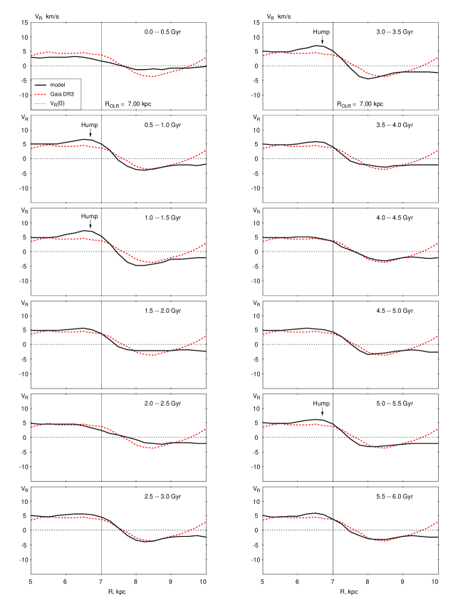
Figure 1 shows the distributions of the model radial velocities along the Galactocentric distance averaged over the time intervals of 0.5 Gyr (50 time instants separated by 10 Myr). Also shown is the distribution of observed velocities derived from the Gaia DR3 data. For building the observed profiles, we used Gaia DR3 stars lying near the Galactic plane, pc, and in a narrow sector of the azimuthal angles, , with known radial velocities and proper motions, the parallax-to-parallax error ratio and the error . To construct the model profiles of the velocity distribution, we used stars of the model disk lying in the sector at different time instants. The median velocities are calculated in -pc wide bins. The method of the determination of the median velocities and their errors is described in Melnik et al. (2021, section 2). The random error in the determination of the observed median velocities calculated in bins in the distance range of 5–10 kpc is, on average, 0.1 km s-1. The similar error calculated for instantaneous model velocities is 0.6 km s-1 but it is reduced to 0.1 km s-1 after averaging over time. On the whole, the profiles show a plateau with km s-1 in the distance range of 5–7 kpc, followed by a smooth fall to the value of km s-1 at the distance of kpc and then a growth or a plateau. We can clearly see that the model velocity increases at the distances 6–7 kpc and forms the hump (elevation) during the time periods 0.5–1.0, 1.0–1.5, 3.0–3.5 and 5.0–5.5 Gyr. The first appearance of the hump lasts long, from 0.6 to 1.8 Gyr, but next humps appear through Gyr and live Gyr. Besides, the height of the humps decreases with time.
We do not present the distributions of the azimuthal velocities here, although they also form humps, which are discussed below.
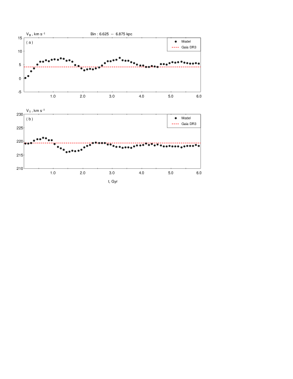
Figure 2 shows the median radial, , and azimuthal, , velocities of model stars in the sector of the azimuthal angles and in one distance bin ( kpc) at different times. The middle of the bin considered is located at the distance kpc. It is this bin where the amplitude of the velocity variations achieves maximum value. We consider all stars of the model disk that fall onto the outlined segment at different time instants. The median velocities and are calculated for 601 time instants separated from each other by 10 Myr and then are averaged over the periods of 100 Myr.
The variations of the velocities are approximated by harmonic oscillations with the period , amplitude , initial phase and the average velocity . The parameters of oscillations of the velocity are derived from the solution of the system of equations:
| (2) |
where are the velocity at the time instants , , .., 60. Eq. (2) can be rewritten in the following way:
| (3) |
We use the standard least square method to solve the system of 61 equations, which are linear in the parameters , and for each value of the nonlinear parameter , and then determine the value of that minimizes the sum of squared normalized deviations . The amplitude and phase are determined by the following expressions:
| (4) |
and
| (5) |
The uncertainty in can be estimated with the use of the uncertainties, and , in the parameters and , respectively:
| (6) |
The parameters of the -velocity oscillations are calculated in a similar way.
Figure 2(a) shows the median velocity of stars lying in the outlined segment of the model disk at different time moments. The average amplitude and initial phase of the -velocity oscillations calculated over the 6 Gyr period is km s-1 and . The average velocity at the 6 Gyr interval is km s-1 which slightly exceeds the velocity derived from the Gaia DR3 data, km s-1. Maximum height of the hump is km s-1. The humps appear for the first, second and third time during the time periods –1.8 Gyr, 3.0–3.8 Gyr and 5.0–5.8 Gyr from the start of simulation, respectively. The height of the humps decreases with time. The period of the -velocity variations is Gyr.
Figure 2(b) shows variations of the median velocity of stars in the indicated segment of the model disk. The average amplitude and initial phase of the -velocity oscillations are km s-1 and . The average velocity is km s-1 which is slightly less than the value derived from Gaia DR3 data, km s-1. The height of the humps also decreases with time. The period of the -velocity variations is Gyr.
Thus, the velocities and calculated for the outlined segment of the model disk, and kpc, demonstrate variations with the period of Gyr. The amplitudes of the velocity variations are 1–2 km s-1 but their statistical significance (the ratio of the amplitude to its uncertainty) exceeds 8.
4 4. Sample of stars creating the humps
4.1 4.1 Selection criterion
We found stars that create the humps on the profiles of the -velocity distributions. Stars captured by the Lindblad resonances often demonstrate the periodic changes in the direction of orbit elongation with respect to the bar major axis (Weinberg, 1994). We selected stars whose orbits are oriented in such a way that they create negative velocities in the region: and –7 kpc, during the certain time periods, and leave this region at other periods.
We calculated the angles , and which determine orbit elongation relative to the bar major axis during the time periods 0–1, 1–2 and 2–3 Gyr from the start of modeling, respectively. Stars that change their orientation as follows: , and appear to contribute significantly in the formation of the humps. Our sample includes 26308 stars, which is only 9% of all stars whose orbits lie both inside and outside the OLR radius.
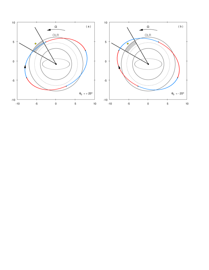
Figure 3 shows two elliptical orbits oriented at the angles (a) and (b) to the major axis of the bar. The change in the orientation of the orbits causes the formation of the humps. The Galaxy rotates counterclockwise, but in the reference system rotating with the bar angular velocity, stars located beyond the CR move clockwise. Orbital segments where stars are approaching () and moving away () from the Galactic center are shown by different colors. The azimuthal angle of the Sun relative to the bar is supposed to be . Also shown is the sector of the azimuthal angles where the velocities are calculated. The segment 6–7 kpc where the humps are forming is highlighted in gray color. We can clearly see that a star moving along the orbit oriented at the angle (Fig. 3a) passes through the region where the humps are forming with a negative radial velocity (). Consequently, such stars “pull” the median velocities towards more negative values and produce pits. When the orbit is oriented at the angle (Fig. 3b), the star passes the Sun at the distance and simply leaves the segment where the humps are forming. It is the escape of stars with the negative velocities, , from the region considered that causes the formation of the humps (see also Section 8).
If a star moves along the elliptical orbit oriented at the angle to the bar major axis, it crosses the Sun–Galactic center line with a zero radial velocity, (Fig. 3). If the orbit is oriented at the angle (), then the star passes the Sun with a negative (positive) radial velocity. The humps appear to be created by stars moving in orbits oriented as follows: , and at the time periods 0–1, 1–2 and 2–3 Gyr, respectively. In other words, these orbits create pits at the time periods 0–1 and 2–3 Gyr and their departure from the region considered causes an increase in the median velocity and the formation of the hump.
Note that the same requirement for the orientation of orbits during the time periods 0–1 Gyr () and 2–3 Gyr () favours selection of orbits with a period of oscillations close, but not strictly equal, to 2 Gyr.
The requirement for the orbit orientation to be at the angle during the time period 1–2 Gyr causes an additional number of stars with negative radial velocities () to appear just outside the OLR, (Fig. 3b). These stars “pull” the median radial velocity calculated in the sector towards more negative values. But the median velocity demonstrates a smooth fall in the distance range kpc (Fig. 1). So the appearance of additional stars with in this area makes this fall sharper.
4.2 4.2 Initial coordinates and velocities of stars creating the humps
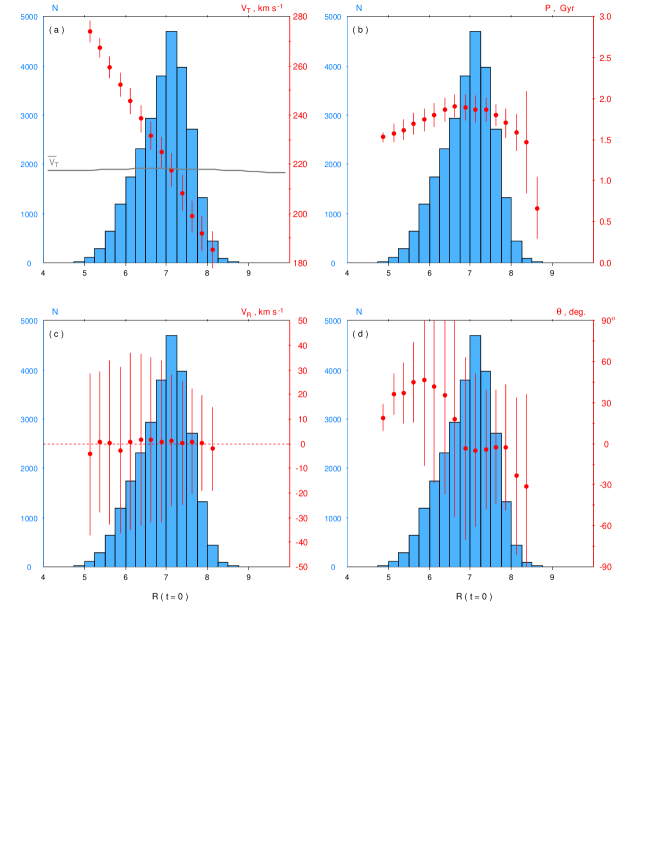
Figure 4 shows the different dependencies obtained for the initial coordinates and velocities of stars creating the humps. It presents the histograms of the star distribution over the distance at the initial time moment () with the distributions of other parameters superimposed upon them. In each bin over , we calculated (a) the median initial azimuthal velocity , (b) the median period of variations of the angular momentum and energy, (c) the median initial radial velocity , and (d) the median initial azimuthal angle . The red vertical lines show median values of dispersion for the corresponding quantities (half central interval containing 67% of objects).
Figure 4(a) shows the dependence of the initial azimuthal velocity, , from the distance . We can clearly see that decreases with increasing . The gray line shows the average initial azimuthal velocity which is calculated from the Jeans equation and is related to all stars located at a given distance at (Melnik et al., 2021, section 3.2). Due to asymmetric drift, the velocity is everywhere less than the velocity of the rotation curve, , and at the OLR radius, their difference amounts to km s-1. The intersection of the gray line and the line drawn through the red circles corresponds to the bin –7.25 kpc, where the majority of stars creating the humps lie at the initial moment.
In general, the decrease in with increasing (Fig. 4a) is easy to understand. Stars creating the humps must cross the OLR radius. So stars located at the smaller (greater) distance than the OLR radius at must “go up” (“go down”) to the OLR radius. So they must have on average greater (smaller) angular momentum, and therefore greater (smaller) azimutulal velocity , than other stars at the corresponding distance.
Figure 4(b) shows changes in the period of variations in the angular momentum and energy obtained for hump-creating stars (see also Section 5). The median period calculated in bins at the distance interval –8.00 kpc lies in the range –1.91 Gyr. The median period calculated for all hump-creating stars is 1.85 Gyr.
Figure 4(c) shows the distribution of the median initial radial velocities, , of hump-creating stars. It is clearly seen that the median velocities are close to zero and lie in the range [, +2] km s-1 at the distance interval –8.50 kpc. As for the dispersion of the radial velocities, it is km s-1 and decreases with increasing distance , which is consistent with the general tendency for the velocity dispersion to decrease on the periphery.
Figure 4(d) shows the median values of the initial azimuthal angles calculated in each bin over the distance . We can clearly see that the angle changes jerkily from +45 to at the distance interval –8.5 kpc, but near the OLR ( kpc), the median angle is close to zero.
5 5. Examples of orbits supporting the humps
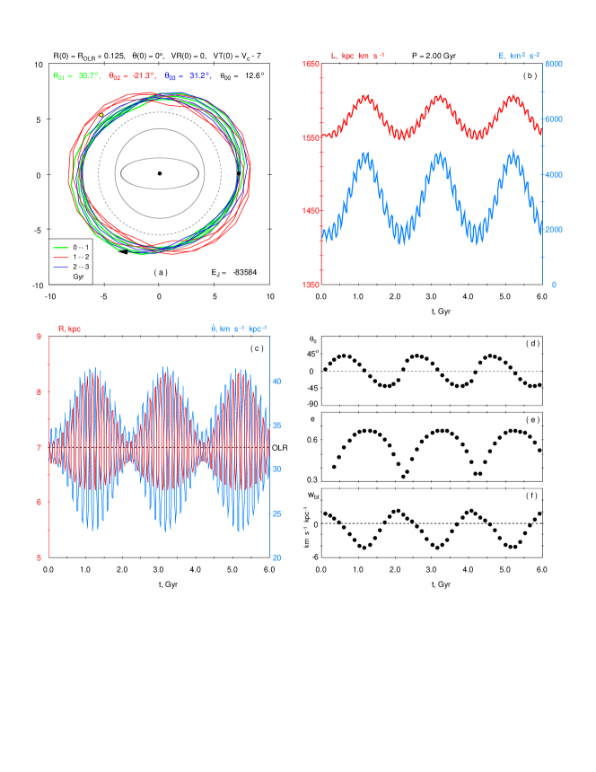
Figure 5(a) shows a typical orbit supporting the humps. The orbit is shown in the reference frame of the rotating bar in which the star considered rotates in the sense opposite that of Galactic rotation. The supposed position of the Sun is shown by the yellow circle. At the initial moment the star is located at the distance of kpc in the direction of the major axis of the bar (black circle) and has radial and azimuthal velocities of and km s-1, which are the most probable values of the velocities and at the given distance at . The angles , and determine the orientation of the orbit relative to the major axis of the bar during the time periods 0–1, 1–2 and 2–3 Gyr, respectively, and satisfy the requirement: , and , which is required for a star to be included in the sample of hump-creating stars. We can clearly see that the orbit of the star is tilted to the right (clockwise) during the time periods 0–1 and 2–3 Gyr and to the left during the period 1–2 Gyr.
The angle determines the orientation of the orbit during the entire time period 0–3 Gyr (Fig. 5a). Since is small, i. e. , we can conclude that the orbit considered generally supports the outer ring stretched parallel to the bar.
In barred galaxies, neither the angular momentum of a star, , nor its total energy, , are conserved, but in the case of a stationary bar, their linear combination is conserved in the form of the Jacobi integral (for example, Binney & Tremaine, 2008):
| (7) |
In our model, the Jacobi integral keeps its value after the bar reaches its full power, , where Gyr. The star considered has km2 s-2, which is saved up to the last digit at .
Figure 5(b) shows variations in the specific angular momentum, , and specific total energy, , of the star considered during the time period 0–6 Gyr. We can clearly see the short- and long-term oscillations in and with the periods of Myr and Myr, respectively. The short-term oscillations arise for all stars and occur twice during a period of revolution of a star relative to the bar. The long-term oscillations have a larger amplitude and arise for stars near the resonances.
Figure 5(c) shows variations in the distance and instantaneous angular velocity . It is clearly seen that the variations in and have the form of beats, which are characterized by periodic changes in amplitudes of oscillations. The star considered crosses the OLR radius at each radial oscillation but the average values of and also demonstrate slow oscillations. Variations in and occur in antiphase.
We divided oscillations of the star into the time intervals from one intersection of the OLR radius with the negative radial velocity, , to another, and calculated the average values of and . An example of such oscillations of and can be found in Melnik et al. (2023, Fig. 11e).
Figure 5(d) shows variations in the angle which determines the direction of the orbit elongation at the time interval of one radial oscillation. The angle is measured from the direction of the bar major axis. It is clearly seen that the angle slowly changes from +45 to and then quickly back.
Figure 5(e) shows variations in the orbital eccentricity, , calculated at the interval of one radial oscillation. The eccentricity takes values in the range –0.67. Note that minimum eccentricity corresponds to minimum average distance .
Figure 5(f) shows variations in the angular frequency of beats, , calculated at the intervals of one radial oscillation. The beat frequency is determined from the relation:
| (8) |
where and change with time. The beat frequency, , is a particular case of the frequency of the resonance (e.g. Chiba, Friske & Schönrich, 2021). For calculation of the epicyclic frequency, , we took into account the correction related to orbital eccentricity (Struck, 2015a, b). Maximum correction to is 0.59 km s-1 kpc-1 which is small compared to the values, –46.4 km s-1 kpc-1. It is seen that takes both positive and negative values which means the change of the sense of the angle shift (see also Section 6.2).
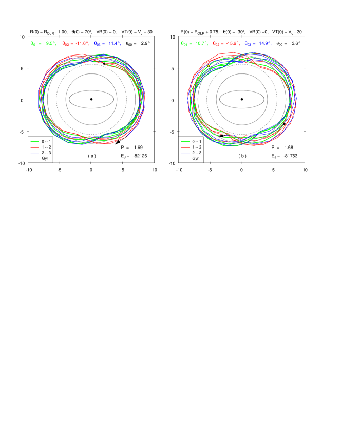
Figure 6 shows two additional examples of hump-creating orbits. Orientations of both orbits during the time periods 0–1, 1–2 and 2–3 Gyr satisfy the criterion , and . At the initial moment, both stars are located at some distance away from the radius OLR: the first star (a) lies closer to the Galactic center, kpc, while the second star (b) lies further away from the center, kpc. To satisfy the above criterion, the initial azimuthal velocities of these stars must differ strongly from the velocity of the rotation curve, . Note that the first (second) star has the initial velocity by 30 km s-1 higher (smaller) than the velocity of the rotation curve at the corresponding distance which reflects the general trend (Fig. 4a).
Figure 6 also shows the periods of variations in the angular momentum and energy of the stars considered which amount to and 1.68 Gyr. Note that these values are a bit smaller than the period of Gyr found for the star shown in Figure 5. This difference also reflects the general trend: the median period decreases as the initial distance of a stars moves away from the OLR radius (Fig. 4b).
Figure 6 also shows the values of the Jacobi integral of the stars considered: and km2 s-2 which have a bit larger values than km2 s-2 of the star shown in Figure 5 (see also Section 7).
Note that the choice of the initial values of the radial velocity and azimuthal angle also affect the period and average orientation of the orbit.
6 6. Statistics of orbits near the OLR
6.1 6.1 Order of symmetry and orientation
We selected 289062 stars whose orbits lie both inside and outside the OLR radius and do not intersect the CR and determined their order of symmetry and, if it is an elliptical orbit (), the direction of the orbit elongation.
To determine the order of symmetry of a stellar orbit, we used the following system of equations:
| (9) |
where and are the Galactocentric distance and the azimuthal angle of the star relative to the major axis of the bar at time moments Myr, where ,.., 300. The values and determine the average Galactocentric distance and average orientation during the time period 0–3 Gyr. This system of equations can be rewritten as follows:
| (10) |
where the angle is derived from the following expression:
| (11) |
and characterizes the average direction of the orbit elongation relative to the major axis of the bar during the time period –3 Gyr. The angle lies in the range and is related to the angle (Section 5) as follows:
| (12) |
We considered the following values of the order of symmetry: , 3, 4 and 5, and calculated the corresponding values of the function (). The value of was adopted to be kpc for all . If one of the four (), for example (), took a value less than other three values by some critical value :
| (13) |
then the order of symmetry of the orbit was chosen to be . If this condition is not satisfied for any then we believed that the shape of the orbit is close to circular, i.e. . The critical value was adopted to be which allows us to select orbits with a certain shape and exclude combined orbits with elements corresponding to different values of .
Table 1 lists the number of orbits with the order of symmetry , 2, 3, 4 and 5 and their fraction from the total sample. For , it also gives the number of orbits oriented in the following sectors: , , , and . For each sample of stars, we calculated the median period and its dispersion, . Table 1 consists of two parts: Part I studies stars whose orbits lie both inside and outside the OLR (289062 stars) and Part II considers the hump-creating stars (26308 stars).
Table 1 (Part I) shows that the majority of orbits, 33.4%, lying both inside and outside the OLR are oriented, on average, perpendicular to the major axis of the bar, , i. e are elongated along the minor axis of the bar. However, the median period calculated for this stars is Myr, therefore, they cannot create the humps with a period of Myr. In addition, the dispersion of periods is Myr here, so this subset of stars cannot produce some organized variations in orbital orientation for a long time.
Quite a lot of stars, 11.1%, have orbits oriented at the angles in the range to the major axis of the bar. The median period and its dispersion are and Myr here. This sample of stars may well create the humps with a period of Myr. The total fraction of orbits oriented along the major axis of the bar, i.e. at the angle in the range is 16.6%.
We paid special attention to orbits with the order of symmetry , as the resonance ( kpc), like the OLR, lies close to the radius where the humps are forming. Table 1 (Part I) shows that the fraction of orbits with is 7.7% which is considerably smaller than the fraction of orbits with (54.8%). The median period for orbits with is Myr. Therefore, these stars cannot create humps with a period of Myr.
The fraction of orbits with the order of symmetry is only 5.7% of all stars near the OLR (Table 1, Part I). However, the median period is quite large, Myr, here. On the other hand, the dispersion of is quite large too, Myr. Generally, these stars can create the humps with a period of Myr but they must quickly dissolve with time.
For completeness, we considered the order of symmetry . The fraction of these orbits is only 3.3% and they do not play a significant role in the hump-formation (Table 1, Part I).
A fairly large fraction of stars, 28.6%, have orbits with the order of symmetry (Table 1, Part I). This means that none of the values of from the range –5 describes these orbits significantly better than others. The median period and dispersion are and Myr here. So this sample of stars cannot create oscillations with a period of Myr.
A different picture is observed for hump-creating stars (Table 1, Part II). Here 71.6% of orbits are stretched in the range of angles . These orbits are, on average, elongated along the major axis bar and support the ring . The median period and dispersion are and Myr here. It is clearly seen that this sample of stars can support the humps with a period of Myr for a long time.
| Part I | ||||
| All orbits lying both in- and outside OLR | ||||
| Myr | Myr | |||
| All | 289062 | 100.0% | 910 | 715 |
| m=2 | ||||
| All | 158332 | 54.8% | 1320 | 695 |
| 32212 | 11.1% | 1730 | 220 | |
| 10122 | 3.5% | 2020 | 210 | |
| 96650 | 33.4% | 780 | 745 | |
| 3316 | 1.1% | 2030 | 560 | |
| 16032 | 5.5% | 1720 | 270 | |
| m=3 | ||||
| All | 22226 | 7.7% | 490 | 130 |
| m=4 | ||||
| All | 16406 | 5.7% | 1930 | 795 |
| m=5 | ||||
| All | 9480 | 3.3% | 650 | 80 |
| m=0 | ||||
| All | 82618 | 28.6% | 720 | 590 |
| Part II | ||||
| Orbits creating the humps | ||||
| Myr | Myr | |||
| All | 26308 | 100.0% | 1850 | 170 |
| m=2 | ||||
| All | 23310 | 88.6% | 1850 | 165 |
| 18824 | 71.6% | 1820 | 155 | |
| 4054 | 15.4% | 1990 | 125 | |
| 0 | 0.0% | – | – | |
| 0 | 0.0% | – | – | |
| 432 | 1.6% | 1460 | 40 | |
| m=3 | ||||
| All | 24 | 0.1% | 650 | 5 |
| m=4 | ||||
| All | 1764 | 6.7% | 1810 | 150 |
| m=5 | ||||
| All | 8 | 0.0% | 1630 | 40 |
| m=0 | ||||
| All | 1202 | 4.6% | 1880 | 555 |
6.2 6.2 Fraction of librating orbits near the OLR
We tried to separate orbits librating within certain angles from orbits which have the direction of elongation shifting only in one direction without any angular restriction. A necessary condition for an orbit to be captured into libration is that it must lie both inside and outside the radius of the resonance. For each of 289062 stars whose orbits lie both inside and outside the OLR, we calculated the values of the beat frequency (Eq. 8). Criterion for orbital libration is following: maximum and minimum values of the beat frequency must be of different signs, and , i.e. the beat frequency must change sign within one oscillation. If does not change sign, then the direction of orbit elongation shifts only in one direction: for – in the sense of Galactic rotation and for – in the opposite sense. The fraction of orbits trapped into libration near the OLR appears to be 28% of orbits lying both inside and outside the OLR.
7 7. Distribution of stars in the plane (, )
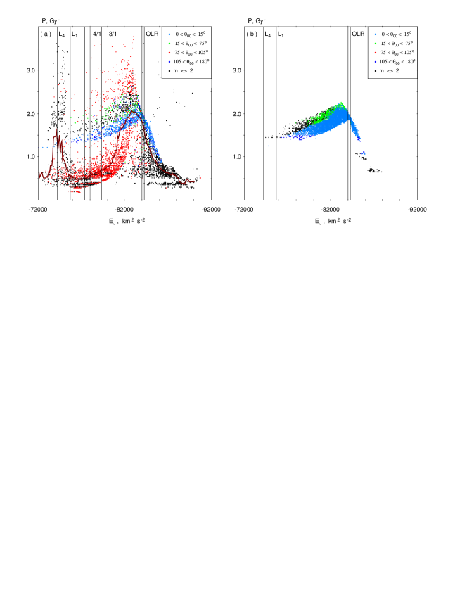
Figure 7 shows the distribution of stars in the plane (, ), where is the Jacobi integral (Eq. 7) and is the period of variations in the angular momentum and total energy. Orientation of orbits with the order of symmetry is shown in color: (blue), (green), (red), (dark blue), where the angle determines the direction of elongation of the orbit relative to the major axis of the bar during the time period 0–3 Gyr. Orbits with the order of symmetry are shown in black.
Figure 7(a) shows the distribution in the plane (, ) built for stars whose orbits lie both inside and outside the OLR (289062 stars). To prevent the overload of the drawing, we present only 2% of stars chosen at random. The solid red curve shows the median period calculated in 100-km2 s-2 wide bins along . The vertical lines show the values of calculated for imaginary stars located at the points and and at the radii of the resonances , and OLR with the velocities and , where is the velocities of the rotation curve at the corresponding radii. The double lines show the values of calculated for stars located on the major (more negative values) and minor axes of the bar. The values of calculated for the OLR radius are (major axis) and km2 s-2 (minor axis). It is clearly seen that the median period increases near the OLR and reaches the value of Gyr and then quickly falls. Also, note a small increase in the median period near the value km2 s-2 corresponding to the equilibrium point .
Figure 7(b) shows the distribution of hump-creating stars (26308 stars) in the plane (, ). It is seen that the majority of stars have orbits oriented at the angle (blue dots) and form a structure resembling an angle: the median period increases practically linearly from to 2.00 Gyr with decreasing from to km2 s-2 and then quickly drops.
8 8. Contribution of hump-creating stars to the oscillations of the velocities and
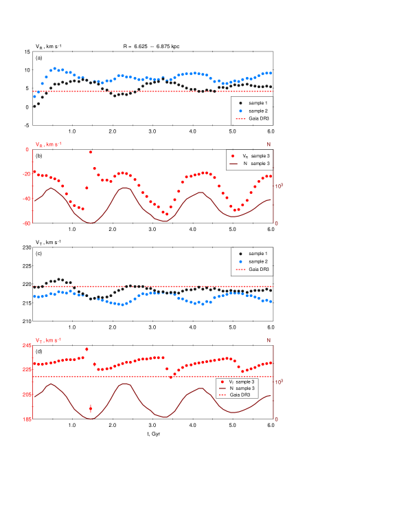
Figure 8 shows the median (a, b) radial and (c, d) azimuthal velocities of model stars lying in the sector of the azimuthal angles and distance bin kpc at different time instants. We consider three samples of stars: (1) all stars of the model disk that fall onto the outlined segment at the moments considered (black circles), (2) all stars of the model disk without hump-creating stars (blue circles), and (3) stars creating the humps (red circles). Also shown are variations in the number of hump-creating stars, , located in the outlined segment of the disk at different times (solid dark-red line).
Figure 8(a) shows variations in the velocity calculated for all stars of the model disk and for the sample without hump-creating stars. We can clearly see that the exclusion of hump-creating stars changed significantly the phase of oscillations of the velocity : pits appear in places of the humps, except for the first one, and humps appear in places of pits.
Let us consider a quantitative criterion characterizing the influence of hump-creating stars on the oscillations of the velocity . A good one is the ratio of the amplitude to its uncertainty . Note that the ratio calculated for all stars located in the outlined segment is (). However, the amplitude computed without hump-creating stars but at the fixed values of the period and phase, i. e. at Gyr and , which determine the positions of the humps and pits for the sample of all stars, is km s-1. We can see that in this case, the amplitude has a value close to its uncertainty and the ratio is . Therefore, variations in the velocity obtained for all stars located in the indicated segment practically disappear after the exclusion of hump-creating stars. However, we can see the appearance of other oscillations in the velocity with humps and pits corresponding to other time moments.
Figure 8(b) shows variations in the velocity and the number of stars obtained for the sample of hump-creating stars (26308 stars). Let us pay attention to the range of the velocity variations: from to 0 km s-1. Besides, minimum velocities correspond to minimum values of . In this case, oscillations of the velocity have the following parameters: Gyr, km s-1, km s-1 and .
A comparison between Fig. 8(a) and Fig. 8(b) shows that the median velocities of hump-creating stars (red circles) are always smaller than the median velocities of all stars in the outlined segment (black circles). The average velocities in the first and second case equal and km s-1, respectively. It means that hump-creating stars “pull” the median velocities towards more negative values. When the number (solid dark-red line) of hump-creating stars increases, their influence becomes more noticeable, and as a result, the median velocities of all stars decrease. Thus, it is the periodic variations in the number of hump-creating stars, , that cause oscillations of the velocity in the outlined segment.
Figure 8(c) shows variations in the velocity calculated for all stars located in the outlined segment (black circles) and for the sample that does not include hump-creating stars (blue circles). It is clearly seen that the exclusion of hump-creating stars shifts, except for the first hump, the phase of oscillations by .
Figure 8(d) shows variations in the median velocity and the number of stars, , calculated for hump-creating stars. We can see that the velocities (red points) lie in the range from 220 to 245 km s-1 except for one time moment ( km s-1) and are shifted towards higher values compared to obtained for all stars lying in the outlined segment. The parameters of the -velocity oscillations calculated for hump-creating stars are follows: Myr, km s-1, km s-1 and . Note that the average velocity , calculated for hump-creating stars ( km s-1) is larger by 11 km s-1 than that obtained for all stars lying in the outlined segment ( km s-1).
A comparison between Fig. 8(c) and Fig. 8(d) shows that variations in the velocity calculated for all stars in the indicated segment (black dots) are in good agreement with oscillations in the number of hump-creating stars (solid dark-red line) which “pull” the median velocity towards higher values. Therefore, an increase in causes a shift in the velocity towards positive values.
The influence of hump-creating stars on the positions of the maxima and minima of the velocity can also be estimated through the ratio of the amplitude to its error . The amplitude calculated for all stars lying in the outlined segment is km s-1 while its value computed without hump-creating stars but at the fixed values of the period and phase, i.e. at Gyr and , is only km s-1. Thus, the ratio drops from 8.9 to 1.4 after the exclusion of hump-creating stars.
Therefore, it is hump-creating stars that cause the variations in the radial and azimuthal velocities with a period of Gyr.
9 9. Distribution of model stars over the period
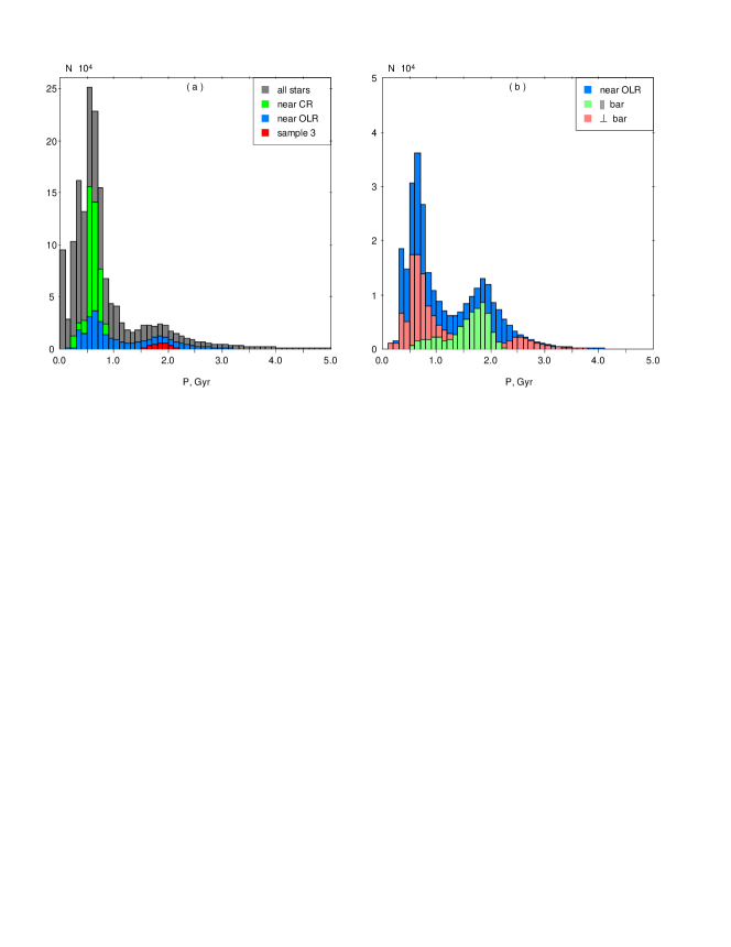
Figure 9 shows the distribution of stars of the model disk over , where is the period of variations in the angular momentum and total energy. Figure 9(a) shows the distributions built for several samples: all stars lying in the model disk; stars whose orbits lie both inside and outside the CR; stars with orbits lying both inside and outside the OLR; and stars creating the humps. We can see two maxima in the distribution of all stars over the period located at and 1.9 Gyr. Stars whose orbits lie both inside and outside the CR concentrate to the first maximum. Note that the period of long-term oscillations near the equilibrium points and equals Myr in our model (Melnik et al., 2023), so the first maximum is likely connected with so-called banana-shaped orbits near the points and . Hump-creating stars concentrate to the second maximum. The distribution of stars whose orbits lie both inside and outside the OLR (289062 stars) also has two maxima. It is shown in an enlarged scale in the right frame.
Figure 9(b) shows that the distribution of stars with orbits lying both inside and outside the OLR also has two maxima located at and Gyr. We identified orbits with the order of symmetry which are oriented perpendicular to the bar () and parallel to the bar (), where the angle determines the average direction of orbit elongation relative to the major axis of the bar during the time period 0–3 Gyr. It is clearly seen that orbits elongated perpendicular to the bar (light-red columns) concentrate to the period while orbits elongated along the bar (light-green columns) – to Gyr. Note that these subsets of orbits support the outer rings and , respectively.
10 10. Age of the Galactic bar
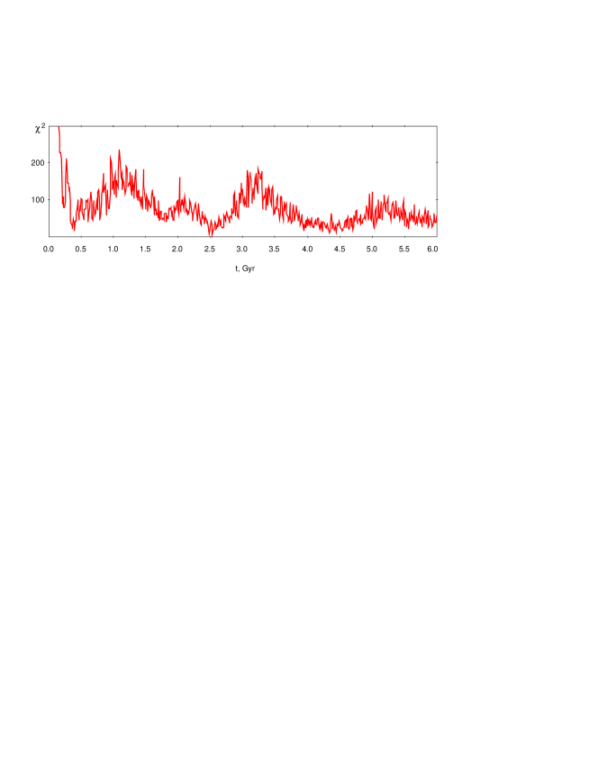
We compared the observed distribution of the median velocity derived from the Gaia DR3 data at the distance interval –9 kpc with the similar model distribution at different time moments and calculated statistics (t). Figure 10 shows the function at the time period 0–6 Gyr. The uncertainty in the median velocity calculated in bins was adopted to be km s-1 (see Section 3). We can see that the function has two minima at the time interval 0.5–6.0 Gyr corresponding to the moments and Gyr. These minima arise due to the disappearance of the humps on the model profiles of the -velocity distributions at the corresponding time periods (Fig. 1). We do not consider the minimum at Gyr, because the bar has not reached its full power by this moment.
The presence or absence of the humps on the model profiles of the -velocity distribution can serve as an indicator of model-observation fit. The observed profile of the -velocity distribution derived from Gaia DR3 data has no hump at the distance interval –7 kpc (Fig. 1). On the other side, the model profiles have the humps at the time periods 0.6–1.8, 3.0–3.8, 5.0–5.8 Gyr. Thus, the best agreement between the model and observations at the time interval 0.5–6.0 Gyr corresponds to the time moments: and Gyr.
From what time moment should we count the age of the bar? In our simulation, there are two critical moments: the start of simulation and the moment when the bar reaches its full power. Real disk galaxies almost always have at least a small oval perturbation in the center, which can exist for a long time. So we will count the age of the bar from the moment it reaches its full power. Since the bar-growth time in our model is Gyr, the age of the bar should be shifted by Gyr towards smaller values with respect to the time moments corresponding to the best agreement between the model and observations. Thus, the age of the Galactic bar counted from the moment of its reaching full strength should be close to one of two values: or Gyr.
11 11. Conclusions
We studied the model of the Galaxy with a bar which reproduces well the distributions of the observed radial, , and azimuthal, , velocities of stars along the Galactocentric distance derived from Gaia DR3 data. For building the observed profiles of the velocity distributions, we used stars lying near the Galactic plane, pc, and in a narrow sector of the azimuthal angles, . The median velocities and were calculated in -pc wide bins. The best agreement between the model and observed velocity profiles corresponds to the angular velocity of the bar km s-1 kpc-1 and the position angle of the bar . In our model the radius of the OLR and the solar Galactocentric radius are located at the distances of and kpc, respectively (Melnik et al., 2023).
We found that the model profiles of the -velocity distribution demonstrate a periodic increase in the velocity at the distance interval 6–7 kpc (Fig. 1). Maximum height of the hump on the -profile equals km s-1 and corresponds to the distance kpc. The height of the humps decreases with time. We studied variations in the velocity in the bin kpc. The average amplitude of the -velocity variations at the time period 0–6 Gyr is km s-1. The period of the hump formation is Gyr (Fig. 2a).
The azimuthal velocity also shows periodic changes in the distance bin kpc. The amplitude and period of the -velocity variations are km s-1 and Gyr (Fig. 2b).
Thus, the velocities and calculated for the segment of the model disk, and kpc, show oscillations with a period of Gyr.
Orbits trapped into librations near the ILR and OLR demonstrate the periodic changes in the direction of orbit elongation (Weinberg, 1994). We calculated the angles , and which determine the direction of orbit elongation relative to the major axis of the bar during the time periods 0–1, 1–2 and 2–3 Gyr from the start of modeling, respectively. We found that stars whose orbits change orientation as follows: , and , make significant contribution to the formation of the humps. During the time periods 0–1 and 2–3 Gyr, the orbits of these stars create negative velocities in the sector and distance range –7 kpc while during the period of 1–2 Gyr, they change their orientation and simply leave the region considered (Fig. 3). The sample of hump-creating stars includes 26308 stars which is only 9% of all stars whose orbits lie both inside and outside the OLR.
We studied the distribution of initial coordinates and velocities of hump-creating stars (Fig. 4). The maximum of the distribution of stars over the initial distance corresponds to the bin –7.25 kpc where maximum number of hump-creating stars is located at . We found the decrease in the initial azimuthal velocity, , with increasing initial distance, . The median initial radial velocities of hump-creating stars are close to zero with the dispersion km s-1.
A typical orbit of hump-creating star is shown in Figure 5. Variations in the angular momentum and total energy demonstrate short- and long-term oscillations with the periods of 0.13 and 2.0 Gyr, respectively. Variations in the distance and instantaneous angular velocity have the form of beats. The angle , which determines the direction of orbit elongation with respect to the major axis of the bar during one radial oscillation, changes in the range from to . The angle , average distance , average angular velocity , orbital eccentricity, and beat frequency, (Eq. 8), change with a period of Gyr.
We studied the order of symmetry and orientation of orbits near the OLR. We selected orbits that lie both inside and outside the OLR and do not cross the CR (289062 stars). Of these, 54.8% have the order of symmetry ; 7.7% – 3; 5.7% – 4 and 3.3% – 5; 28.6% orbits have the shape close to circular. The majority of orbits with the order of symmetry are stretched perpendicular to the bar () which amounts to 33.4% of the total sample. The fraction of orbits elongated along the bar () is only 16.6% (Table 1, Part I).
Among hump-creating stars (26308 stars), 88.6% have orbits with the order of symmetry . The majority (71.6%) of orbits with are oriented along the bar at the angle . Thus, the majority of hump-creating stars support the outer ring . The median period calculated for hump-creating stars is Gyr (Table 1, Part II).
The fraction of librating orbits that change the direction of their elongation within a certain range of angles, , amounts to 28% of all orbits lying both inside and outside the OLR (Section 6.2).
We studied the distribution of stars whose orbits lie both inside and outside the OLR in the plane (, ). It appears that the median period increases with decreasing and approaching the OLR and then drops sharply. Hump-creating stars demonstrate this tendency even more clearly (Fig. 7).
We explored the influence of hump-creating stars on the oscillations of the median radial velocity of stars lying in the disk segment: and kpc (Fig. 8). The exclusion of hump-creating stars significantly changes the phase of the oscillations: pits appear in places of the humps, except for the first one, and humps arises in places of the pits. The ratio of the amplitude and its uncertainty, , calculated for the sample without hump-creating stars under the fixed period and phase equals which is significantly smaller than the ratio obtained for all stars lying in the outlined segment, .
A similar test made for the azimuthal velocity showed that the exclusion of hump-creating stars under the fixed period and phase leads to a decrease in the ratio from 8.9 to 1.4.
The distribution of stars of the model disk over the period has two maxima lying at and 1.9 Gyr (Fig. 9a). Stars whose orbits lie both inside and outside the CR concentrate to the first maximum. Note that the period of Gyr practically coincides with the period of long-term oscillations around the equilibrium points and , so the first maximum is likely connected with so-called banana-shaped orbits. The distribution of stars whose orbits lie both inside and outside the OLR also has two maxima: at and 1.9 Gyr. Among them, orbits elongated perpendicular and parallel to the bar concentrate to the first and second maxima, respectively. These orbits support the outer rings and , respectively (Fig. 9b).
A comparison between the model and observed distributions of the velocity showed that the function has two minima corresponding to the time moments and Gyr (Fig. 10) which arise due to the disappearance of the humps on the model profiles of the -velocity distribution. Thus, the age of the Galactic bar counted from the moment of its reaching full power must lie near one of two values: or Gyr.
Acknowledgements
We thank the anonymous referees for useful remarks
and interesting discussion. This work has made use of data from the
European Space Agency (ESA) mission Gaia
(https://www.cosmos.esa.int/gaia), processed by the Gaia
Data Processing and Analysis Consortium (DPAC, https:
//www.cosmos.esa.int/web/gaia/dpac/consortium). Funding for
the DPAC has been provided by national institutions, in particular
the institutions participating in the Gaia Multilateral
Agreement. E.N. Podzolkova is a scholarship holder of the Foundation
for the Advancement of Theoretical Physics and Mathematics ”BASIS”
(Grant No. 21-2-2-44-1).
References
- Antoja et al. (2014) Antoja, T. ; Helmi, A. ; Dehnen, W., et al., 2014, A&A, 563, 60
- Asano et al. (2022) Asano, T., Fujii, M. S., Baba, J., Bédorf, J., Sellentin, E., Portegies Zwart, S., 2022, MNRAS, 514, 460
- Athanassoula (1992) Athanassoula E. 1992, MNRAS, 259, 328
- Athanassoula et al. (1983) Athanassoula, E., Bienayme, O., Martinet, L., Pfenniger, D., 1983, A&A, 127, 349
- Benjamin et al. (2005) Benjamin, R. A., Churchwell, E., Babler, B. L., et al. 2005, ApJ, 630, L149
- Bensby et al. (2017) Bensby, T., Feltzing, S., Gould, A., et al., 2017, A&A, 605 A89
- Bica et al. (2006) Bica, E., Bonatto, C., Barbuy, B., Ortolani, S., 2006, A&A, 450, 105
- Binney & Tremaine (2008) Binney, J., Tremaine, S., Galactic Dynamics, Second Edition, Princeton Univ. Press, Princeton, New Jersey, 2008.
- Block et al. (2001) Block, D. L., Puerari, I., Knapen, J. H., et al., 2001, A&A, 375, 761
- Boehle et al. (2016) Boehle, A., Ghez, A. M., Schödel, R. et al. 2016, ApJ, 830, 17
- Bovy et al. (2019) Bovy, J., Leung, H. W., Hunt, J. A., et al., 2019, MNRAS, 490, 4740
- Branham (2017) Branham, R. L. 2017, Ap&SS, 362, 29
- Buta (1995) Buta, R. 1995, ApJS, 96, 39
- Buta & Combes (1996) Buta, R., Combes, F. 1996, Fund. Cosmic Physics, 17, 95
- Buta & Crocker (1991) Buta, R., Crocker, D. A. 1991, AJ, 102, 1715
- Buta, Laurikainen & Salo (2004) Buta, R., Laurikainen, E., Salo, H. 2004, AJ, 127, 279
- Byrd et al. (1994) Byrd, G., Rautiainen, P., Salo, H., Buta, R., Crocker, D. A. 1994, AJ, 108, 476
- Cabrera-Lavers et al. (2007) Cabrera-Lavers, A., Hammersley, P. L., González-Fernández, C., et al. 2007, A&A, 465, 825
- Chiba, Friske & Schönrich (2021) Chiba, R., Friske, J., Schönrich, R. 2021, MNRAS, 500, 4710
- Cole & Weinberg (2002) Cole, A. A., Weinberg, M. D., 2002, ApJ, 574, L43
- Contopoulos (1983) Contopoulos, G. 1983, Celest. Mechan., 31, 193
- Contopoulos & Grosbol (1989) Contopoulos, G., Grosbol, P. 1989, A&AR, 1, 261
- Contopoulos & Papayannopoulos (1980) Contopoulos, G., Papayannopoulos, Th. 1980, A&A, 92, 33
- Dambis et al. (2013) Dambis, A. K., Berdnikov, L. N., Kniazev, A. Y., et al. 2013, MNRAS, 435, 3206
- Debattista et al. (2019) Debattista, V. P., Gonzalez, O. A., Sanderson, R. E., et al., 2019, MNRAS, 485, 5073
- Dehnen (2000) Dehnen, W., 2000 AJ, 119, 800
- de Vaucouleurs & Freeman (1972) de Vaucouleurs, G., Freeman, K. C. 1972, Vis. in Astron., 14, 163
- Díaz-García et al. (2016) Díaz-García, S., Salo, H., Laurikainen, E., Herrera-Endoqui, M. 2016, A&A, 587, 160
- Dwek et al. (1995) Dwek, E., Arendt, R. G., Hauser, M. G., et al. 1995, ApJ, 445, 716
- Eisenhauer et al. (2005) Eisenhauer, F., Genzel, R., Alexander, T., et al. 2005, ApJ, 628, 246
- Feast et al. (2008) Feast, M. W., Laney, C. D., Kinman, T. D., van Leeuwen, F., Whitelock, P. A. 2008, MNRAS, 386, 2115
- Francis & Anderson (2014) Francis, Ch., Anderson, E. 2014, MNRAS, 441, 1105
- Fujii et al. (2019) Fujii, M. S., Bédorf, J., Baba, J., Portegies Zwart, S. 2019, MNRAS, 482, 1983
- Gaia Collaboration, Brown, Vallenari et al. (2021) Gaia Collaboration, Brown, A. G. A., Vallenari, A., et al. 2021, A&A, 649, A1
- Gaia Collaboration, Katz, Antoja et al. (2018) Gaia Collaboration, Katz, D., Antoja, T., et al. 2018, A& A, 616, A11
- Gaia Collaboration, Prusti, de Bruijne et al. (2016) Gaia Collaboration, Prusti, T., de Bruijne, J. H. J., et al. 2016, A&A, 595, A1
- Gaia Collaboration, Vallenari, Brown et al. (2023) Gaia Collaboration, Vallenari, A., Brown, A. G. A., et al. 2023, A&A, 674, A1
- Gerhard (2011) Gerhard, O. 2011, Mem. S. A. It. Suppl., 18, 185
- Glushkova et al. (1998) Glushkova, E. V., Dambis, A. K., Melnik, A. M., Rastorguev, A. S. 1998, A&A, 329, 514
- González-Fernández et al. (2012) González-Fernández, C., López-Corredoira, M., Amôres, E. B., Minniti, D., Lucas, P., Toledo, I. 2012, A&A, 546, 107
- Groenewegen, Udalski & Bono (2008) Groenewegen, M. A. T., Udalski, A., Bono, G. 2008, A&A, 481, 441
- Hasselquist et al. (2020) Hasselquist, S., Zasowski, G., Feuillet, D. K., et al., 2020, ApJ, 901, 109
- Iwanek et al. (2023) Iwanek, P., Poleski, R., Kozlowski, S., et al. 2023, ApJS, 264, 20
- Kalnajs (1991) Kalnajs, A. J., 1991, in Sundelius B., ed., Dynamics of Disc Galaxies. Göteborgs Univ., Göthenburg, p. 323
- Lindegren, Klioner, Hernandez et al. (2021) Lindegren, L., Klioner, S. A., Hernandez, J., et al. 2021, A&A, 649, A2
- Melnik (2019) Melnik, A. M. 2019, MNRAS, 485, 2106
- Melnik & Dambis (2020) Melnik, A. M., Dambis, A. K., 2020, Ap&SS, 365, 112
- Melnik et al. (2021) Melnik, A. M., Dambis, A. K., Podzolkova, E. N., Berdnikov, L. N. 2021, MNRAS, 507, 4409
- Melnik et al. (2023) Melnik, A. M., Podzolkova, E. N., Dambis, A. K. 2023, MNRAS, 525, 3287
- Melnik & Rautiainen (2009) Melnik, A. M., Rautiainen, P. 2009, Astron. Lett., 35, 609
- Melnik & Rautiainen (2011) Melnik, A. M., Rautiainen, P. 2011, MNRAS, 418, 2508
- Melnik et al. (2015) Melnik, A. M., Rautiainen, P., Berdnikov, L. N., Dambis, A. K., Rastorguev, A. S. 2015, AN, 336, 70
- Melnik et al. (2016) Melnik, A. M., Rautiainen, P., Glushkova, E. V., Dambis, A. K. 2016, Ap&SS, 361, 60
- Minchev et al. (2007) Minchev, I., Nordhaus, J., Quillen, A. C., 2007, ApJ, 664, L31
- Monari et al. (2017) Monari, G., Famaey, B., Siebert, A., Duchateau, A., Lorscheider, T., Bienayme, O. 2017, MNRAS, 465, 1443
- Nataf (2016) Nataf D. M. 2016, PASA, 33, 23
- Nataf (2017) Nataf D. M. 2017, PASA, 34, 41
- Nepal et al. (2024) Nepal, S., Chiappini, C., Guiglion, G., et al., 2024, A&A, 681, L8
- Ness & Lang (2016) Ness, M., Lang, D. 2016, AJ, 152, 14
- Nikiforov (2004) Nikiforov, I. I. 2004, ASP Conf. Ser. Vol. 316, Astron. Soc. Pac., San Francisco, p. 199
- Nishiyama et al. (2006) Nishiyama, S., Nagata, T., Sato, S., et al. 2006, ApJ, 647, 1093
- Pfenniger (1984) Pfenniger, D. 1984, A&A, 134, 373
- Rautiainen & Melnik (2010) Rautiainen, P., Melnik, A. M. 2010, A&A, 519, 70
- Rautiainen & Salo (1999) Rautiainen, P., Salo, H. 1999, A&A, 348, 737
- Rautiainen & Salo (2000) Rautiainen, P., Salo, H. 2000, A&A, 362, 465
- Reid et al. (2009) Reid, M. J., Menten, K. M., Zheng, X. W., Brunthaler, A., Xu, Y. 2009, ApJ, 705, 1548
- Sanders et al. (2024) Sanders, J. L., Kawata, D., Matsunaga, N., Sormani, M. C., Smith, L. C., Minniti, D., Gerhard, O. 2024, MNRAS, 530, 2972
- Schwarz (1981) Schwarz, M. P. 1981, ApJ, 247, 77
- Sellwood & Wilkinson (1993) Sellwood, J. A., Wilkinson, A. 1993, Rep. on Prog. in Phys., 56, 173
- Shen et al. (2010) Shen, J., Rich, R. M., Kormendy, J., et al. 2010, ApJ, 720, L72
- Struck (2015a) Struck, C. 2015, MNRAS, 446, 3139
- Struck (2015b) Struck, C. 2015, MNRAS, 450, 2217
- Trick et al. (2021) Trick, W. H., Fragkoudi, F., Hunt, J. A. S., Mackereth, J. T., White, S. D. M. 2021, MNRAS, 500, 2645
- Weinberg (1994) Weinberg, M. D. 1994, ApJ, 420, 597