Accumulator-Aware Post-Training Quantization

Abstract

Several recent studies have investigated low-precision accumulation, reporting improvements in throughput, power, and area across various platforms. However, the accompanying proposals have only considered the quantization-aware training (QAT) paradigm, in which models are fine-tuned or trained from scratch with quantization in the loop. As models continue to grow in size, QAT techniques become increasingly more expensive, which has motivated the recent surge in post-training quantization (PTQ) research. To the best of our knowledge, ours marks the first formal study of accumulator-aware quantization in the PTQ setting. To bridge this gap, we introduce AXE—a practical framework of accumulator-aware extensions designed to endow overflow avoidance guarantees to existing layer-wise PTQ algorithms. We theoretically motivate AXE and demonstrate its flexibility by implementing it on top of two state-of-the-art PTQ algorithms: GPFQ and OPTQ. We further generalize AXE to support multi-stage accumulation for the first time, opening the door for full datapath optimization and scaling to large language models (LLMs). We evaluate AXE across image classification and language generation models, and observe significant improvements in the trade-off between accumulator bit width and model accuracy over baseline methods.

1 Introduction

Modern deep learning models have scaled to use billions of parameters, requiring billions (or even trillions) of multiply-accumulate (MAC) operations during inference. Their enormous size presents a major obstacle to their deployment as their compute and memory requirements during inference often exceed the budgets of real-world systems. As a result, model compression has emerged as an active area in deep learning research, with quantization being among the most prevalent techniques studied in literature [1, 2, 3] and applied in practice [4, 5, 6].

Quantization techniques commonly reduce the inference costs of a deep learning model by restricting the precision of its weights and activations. Although substituting the standard 32-bit floating-point operands for low-precision counterparts can drastically reduce the cost of multiplications, this only accounts for part of the core MAC operation; the resulting products are often still accumulated using 32-bit additions. Recent studies have demonstrated that also restricting the precision of the accumulator can yield significant benefits [7, 8, 9, 10, 11]. For example, de Bruin et al. [8] and Xie et al. [9] both show that 16-bit integer accumulation on ARM processors can yield nearly a $2\times$ throughput increase over 32-bit, and Ni et al. [7] show that further reducing to 8-bit accumulation on custom ASICs can improve energy efficiency by over $4\times$. However, exploiting such an optimization is non-trivial in practice as reducing the width of the accumulator exponentially increases the risk of numerical overflow, which is known to introduce arithmetic errors that significantly degrade model accuracy [7, 12].

To address this, recent work has proposed an accumulator-aware quantization paradigm that entirely eliminates the risk of numerical overflow via strict learning constraints informed by theoretical guarantees [12]. The resulting scope of investigations has been limited to the quantization-aware training (QAT) setting in which models are trained from scratch or fine-tuned from checkpoints with quantization in the loop [12, 13]. With the rising training costs of modern deep learning models (e.g., large language models), it is important to develop methods that are equally as effective in the post-training quantization (PTQ) setting, where pre-trained models are directly quantized and calibrated using relatively modest resources. However, as further discussed in Section 2, controlling the accumulator bit width in such a scenario is non-trivial. In this work, we characterize and address these challenges, introduce a practical framework for their investigation, and establish a new state-of-the-art for accumulator-aware quantization in the PTQ setting.

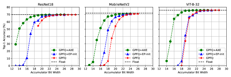
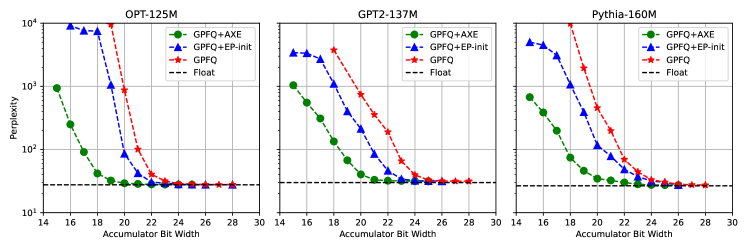
Figure 1: To reduce the minimum accumulator bit width required to avoid overflow during inference, one could heuristically manipulate the weight and activation bit widths according to the data type bound derived in [12]. To date, Euclidean projection-based initialization (EP-init) [13] serves as the best alternative to this approach, but, as the name suggests, it has only been studied as an initialization strategy for QAT. When applied to GPFQ [14], our framework (green circles) significantly improves the trade-off between accumulator bit width and model accuracy when compared to EP-init [13] (blue triangles) and naïve bit width manipulation (red stars) on image classification models evaluated on ImageNet [15] (top) and language generation models evaluated on WikiText2 [16] (bottom).

Contribution. We introduce AXE, a framework of accumulator-aware extensions designed to endow overflow avoidance guarantees to any layer-wise PTQ algorithm that greedily quantizes weights one at a time, provided the base algorithm is also amenable to activation quantization. We theoretically motivate AXE and demonstrate its flexibility by presenting accumulator-aware variants of both GPFQ [14] and OPTQ [17]. We evaluate AXE across pre-trained image classification and language generation models and show that it significantly improves the trade-off between accumulator bit width and model accuracy when compared to baseline methods. We visualize this trade-off using Pareto frontiers, as in Figure 1 with GPFQ, which provide the maximum observed model accuracy for a given target accumulator bit width; we provide additional results with OPTQ in Section 4.1. Furthermore, unlike prior accumulator-aware quantization methods, which assume a monolithic accumulator, we generalize AXE to support multi-stage accumulation and extend accumulator-aware quantization to large language models (LLMs) for the first time. Indeed, our results show that AXE scales extremely well within the Pythia model suite [18] when targeting multi-stage accumulation, supporting the scaling hypothesis proposed in [13].

Broader Impact. Just as the benefits of reducing weight and activation bit widths are non-uniform across platforms (e.g., 3-bit weights are hard to accelerate on conventional platforms), the benefits of reduced accumulator bit widths often depend on some combination of compiler-level software support, instruction sets of the target platform, and availability of suitable datapaths in hardware. Prior works have motivated accumulator bit width reduction and characterized inference cost improvements across many dimensions on different platforms, as we discuss further in Section 2.2. Our intention in this work is to directly extend the scope of accumulator-aware quantization to the PTQ setting without dependence on the capabilities of a single target platform. We hope that our work will stimulate further research in both accumulator-aware quantization and low-precision accumulation.

2 Preliminaries

We denote the intermediate activations of a neural network with $L$ layers as $\{\bm{x}^{(l)}\}_{l=1}^{L}$, where $\bm{x}^{(l)}\in\mathbb{R}^{K_{l}}$ denotes the $K_{l}$-dimensional input activations to layer $l$, and $\bm{X}^{(l)}\in\mathbb{R}^{K_{l}\times D}$ denotes a matrix of $D$ such inputs. The set of weights for the network is similarly denoted as $\{\bm{W}^{(l)}\}_{l=1}^{L}$, where $\bm{W}^{(l)}\in\mathbb{R}^{C_{l}\times K_{l}}$ denotes the weight matrix for layer $l$ with $K_{l}$ input neurons and $C_{l}$ output neurons; its quantized counterpart is denoted as $\bm{Q}^{(l)}\in\mathcal{A}^{C_{l}\times K_{l}}_{M}$, where we adopt the notation $\mathcal{A}^{m\times n}_{b}$ to denote the space of all $m\times n$ matrices whose elements are part of a fixed $b$-bit alphabet defined by the target quantization space. For example, $\mathcal{A}_{b}:=\{k:-2^{b-1}+1\leq k\leq 2^{b-1}-1,k\in\mathbb{Z}\}$ is the alphabet of signed $b$-bit integers, assuming a sign-magnitude representation, where $\mathbb{Z}$ is the space of all scalar integers.

For layer $l$, our notation yields $C_{l}$ independent dot products of depth $K_{l}$ for each of the $D$ inputs. For clarity, and without loss of generality, we often assume $C_{l}=1$ when focusing on a single layer $l$ so that we can use $\bm{w}^{(l)}$ to denote the weight matrix for layer $l$, with $w_{i}^{(l)}$ denoting a single weight element. When dropping their superscript, $\bm{x}$ and $\bm{w}$ denote generic inputs and weights in $\mathbb{R}^{K}$, and $\bm{\tilde{x}}$ and $\bm{q}$ denote their quantized counterparts.

2.1 Post-Training Quantization

Standard quantization operators, referred to as quantizers, are commonly parameterized by zero-point $z$ and strictly positive scaling factor $s$, as shown in Eq. 1 for weight tensor $\bm{w}$. Our work focuses on uniform integer quantization, where $z$ is an integer value that ensures that zero is exactly represented in the quantized domain, and $s$ is a strictly positive scalar that corresponds to the resolution of the quantizer. Scaled values are commonly rounded to the nearest integer, denoted by $\lceil\cdot\rfloor$, and elements that exceed the representation range of the quantized domain $\mathcal{A}_{b}$ are clipped.

$$\mathcal{Q}(\bm{w}):=s\cdot\left(\text{clip}\left(\left\lceil\frac{\bm{w}}{s}\right\rfloor+z;\min\mathcal{A}_{b},\max\mathcal{A}_{b}\right)-z\right)$$ (1)

Methods for tuning these quantizers broadly fall into two paradigms: quantization-aware training (QAT) and post-training quantization (PTQ). QAT methods train or fine-tune a neural network with quantization in the loop, which often requires significant compute resources and sufficiently large datasets [2, 3]. Our work focuses on PTQ methods, which directly cast and calibrate pre-trained models and often rely on little to no data without end-to-end training [2, 3]. PTQ methods tend to follow a similar general structure [14, 17, 19], greedily casting and calibrating quantized models layer-by-layer or block-by-block while seeking to approximate the minimizer of the reconstruction error

$$\bm{q}^{*}=\operatorname*{arg\,min}_{\bm{q}}\frac{1}{2}\|\bm{X}^{T}\bm{w}-\bm{\tilde{X}}^{T}\bm{q}\|^{2}_{2}$$ (2)

where $\bm{q}^{*}$ is the optimal quantized weights and $\bm{\tilde{X}}$ is the quantized counterpart of $\bm{X}$. Recent PTQ methods concentrate on “weight-only quantization”, where $\bm{\tilde{X}}=\bm{X}$, to solely minimize memory storage and transfer costs [14, 17, 19], and for good reason—the ever-increasing weight volume of state-of-the-art neural networks has rendered many hyper-scale transformer models memory-bound [20, 18, 21, 22]. In such a scenario, weight-only quantization algorithms can better preserve model quality and still realize end-to-end throughput gains just by reducing data transfer costs, even with high-precision computations (usually FP16) [17, 23]. However, weight-only quantization provides limited opportunity to accelerate compute-intensive operations such as matrix multiplications, which is the focus of this work. Thus, we investigate methods that are amenable to quantizing both weights and activations to low precision integers, which can realize throughput gains from both accelerated computation and reduced data traffic [24, 25]. Some methods aim to solve this problem by tuning quantization parameters through iterative graph equalization [26, 27, 24, 28] or local gradient-based reconstruction [29, 30, 31], other methods such as GPFQ [14] and OPTQ [17] (formally GPTQ) quantize weights one-by-one while greedily adjusting for quantization error. We find that these greedy sequential quantization algorithms are particularly amenable to accumulator-awareness, as we discuss further in Section 3.

2.2 Low-Precision Accumulation

The majority of neural network quantization research targeting compute acceleration emphasizes low-precision weights and activations. While this can significantly reduce the costs of multiplications, the resulting products are often still accumulated using high-precision additions. As lower precision integer representations continue to increase in popularity [32, 33], one can expect a focus skewed towards weight and activation quantization to yield diminishing returns as high-precision additions can bottleneck throughput, power, and area [7, 8, 9, 13]. For example, Ni et al. [7] show that when constraining weights and activations to 3-bit $\times$ 1-bit multipliers, the cost of 32-bit accumulation consumes nearly 75% of the total power and 90% of the total area of their custom MAC unit; they report up to 4$\times$ power savings and 5$\times$ area reduction when reducing to 8-bit accumulation.

Reducing the accumulator bit width is non-trivial in practice as it exponentially increases the risk of numerical overflow [12], often introducing arithmetic errors that degrade model accuracy [7, 12]. Existing methods to prepare quantized neural networks (QNNs) for low-precision accumulation often aim to either reduce the risk of numerical overflow [9, 34, 35] or mitigate its impact on model accuracy [7, 36, 37]. These empirical approaches rely on several assumptions that limit their real-world applicability. For one, as discussed in [13], empirical estimates of overflow rely on a priori knowledge of the input distribution, which is impractical to assume in many real-world scenarios and can even introduce vulnerabilities [38]. Furthermore, overflow behavior can vary across platforms and programming languages, so designing methods to mitigate the detrimental impact of one particular overflow behavior (e.g., wraparound two’s complement arithmetic) limits portability across applications and accelerators. Finally, empirical approaches are unable to support applications that require guaranteed arithmetic correctness, such as encrypted inference [39, 40], and are known to break down when overflows occur too frequently [7]. To address these concerns, recent work has proposed to avoid overflow altogether using accumulator-aware quantization (A2Q) [12, 13].

2.3 Accumulator-Aware Quantization

Let $P^{*}$ denote the minimum accumulator bit width required to guarantee overflow avoidance for a given dot product. Aside from universally fixing the accumulator at 32 bits (or any other arbitrary maximum number of bits imposed by a given processor), the most conservative method to calculate $P^{*}$ considers the data types of the dot product operands, i.e., weights and activations. Given inputs $\tilde{\bm{x}}\in\mathcal{A}^{K}_{N}$ and weights $\bm{q}\in\mathcal{A}^{K}_{M}$, $P^{*}$ is given by Eq. 3 as derived in [12], where $\mathbbm{1}_{\text{signed}}(\tilde{\bm{x}})$ is an indicator function that returns 1 if $\tilde{\bm{x}}$ is signed and 0 otherwise.

$$P^{*}=\left\lceil\log_{2}\left(2^{\log_{2}(K)+N+M-1-\mathbbm{1}_{\text{signed}}(\tilde{\bm{x}})}+1\right)+1\right\rceil$$ (3)

Note that $P^{*}$ increases linearly with the bit widths of the operands and logarithmically with the depth of the dot product. Thus, for a fixed neural architecture, one could heuristically manipulate the weight and activation bit widths according to Eq. 3 to reduce $P^{*}$. However, the quantization design space ultimately limits the minimum attainable accumulator bit width, as well as the maximum attainable model accuracy for any target accumulator bit width [12, 13].

Colbert et al. [13] show that one can directly target the accumulator bit width as an independent dimension of the quantization design space while still theoretically guaranteeing overflow avoidance. When accumulating $\tilde{\bm{x}}^{T}\bm{q}$ into a signed $P$-bit accumulator, one need only constrain $\|\bm{q}\|_{1}$ according to Eq. 4, assuming that $\textstyle\sum_{i}q_{i}=0$.

$$\|\bm{q}\|_{1}\leq\frac{2^{P}-2}{2^{N}-1}$$ (4)

Motivated by this result, accumulator-aware QAT methods avoid overflow by constraining the $\ell_{1}$-norm of weights during training to ultimately restrict the range of dot product outputs during inference [12, 13]. These approaches rely on weight normalization-based quantizers infused with strict accumulator-aware learning constraints. Although these approaches have yielded promising results in low-precision accumulation scenarios, the scope of their success is limited to the QAT setting [12, 13]. However, from this family of QAT methods, one can apply the Euclidean projection-based initialization strategy (EP-init) to the PTQ setting without modification as proposed in [13]. However, we find that EP-init has two shortcomings in the PTQ setting: (1) it universally relies on the round-to-zero rounding function to ensure that $|Q(w_{i})|\leq|w_{i}|$ for all $i$ [12, 13]; and (2) it is a vector-wise projection operation that is not amenable to error correction (see Appendix C.2). We address both of these shortcomings in this work.

3 Accumulator-Aware Post-Training Quantization

The standard problem for neural network quantization aims to map high-precision values (e.g., 32-bit floating-point) to low-precision counterparts (e.g., 4-bit scaled integers) while locally minimizing the discrepancy between the output of the original model and that of the compressed one, as formalized by Eq. 2 in Section 2.1. In the post-training quantization (PTQ) setting, one often assumes the quantizer parameters (i.e., scaling factor $s$ and zero point $z$) are fixed and that the individual weights can move freely, as in [14, 17, 41]. Building from this, we formalize accumulator-aware quantization as a constrained variant of the standard reconstruction problem in which the optimal quantized weights $\bm{q}^{*}$ minimize local quantization error while also satisfying a strict $\ell_{1}$-norm constraint, as defined below.

$$\bm{q}^{*}=\operatorname*{arg\,min}_{\bm{q}}\frac{1}{2}\|\bm{X}^{T}\bm{w}-\bm{\tilde{X}}^{T}\bm{q}\|^{2}_{2}\quad\textrm{s.t.}\quad\|\bm{q}\|_{1}\leq Z$$ (5)

To approximately solve this accumulator-constrained reconstruction problem, we introduce AXE, a practical low-overhead framework of general accumulator-aware extensions that endow guaranteed overflow avoidance to layer-wise quantization algorithms that greedily assign bits element-by-element, e.g., GPFQ [14] and OPTQ [17]. AXE is built on two accumulator-aware constraints: (1) a soft global constraint that discourages the underlying algorithm from opportunistically selecting quantized weights with high magnitudes; and (2) a strict local constraint that greedily limits the range of each selected quantized weight while error is iteratively corrected. In its standard form, AXE applies these constraints per-channel (or per-neuron) so that each dot product in the network is guaranteed to independently avoid overflow. Furthermore, without violating our constraints, we generalize our framework to also support multi-stage accumulation in the form of tiled dot products by applying our constraints in finer granularities. We first theoretically justify our solution using GPFQ, then provide accumulator-aware variants of both GPFQ and OPTQ.

3.1 Accumulator Constraints without Zero-Centering

Our goal is to provide a theoretical guarantee of overflow avoidance when accumulating the dot product of $\bm{q}$ by any $\tilde{\bm{x}}\in\mathcal{A}^{K}_{N}$ into a signed $P$-bit register. As discussed in Section 2.3, if $\bm{q}$ is a zero-centered vector such that $\textstyle\sum_{i}q_{i}=0$, then it is sufficient to constrain $\|\bm{q}\|_{1}$ to satisfy the upper bound given by Eq. 4 in order to guarantee overflow avoidance. However, enforcing such a zero-centering constraint on a vector of integers is non-trivial in practice. Rather than directly enforcing this constraint on $\bm{q}$, A2Q+ [13] enforces these constraints on its floating-point counterpart $\bm{w}$ and relies on the symmetry of the quantizer and the round-to-zero operator to ensure that $|Q(w_{i})|\leq|w_{i}|$ for all $i$. We detach our solution from the zero-centering, round-to-zero, and symmetrical constraints of A2Q+.

For any $\tilde{\bm{x}}\in\mathcal{A}^{K}_{N}$, each element $\tilde{x}_{i}$ lies within the closed interval $[\mu,\nu]$ for all $i=\{1,\cdots,K\}$, and $\nu-\mu=2^{N}-1$. It follows that the maximizing vector, $\bm{u}=\operatorname*{arg\,max}_{\tilde{\bm{x}}}\tilde{\bm{x}}^{T}\bm{q}$, and the minimizing vector, $\bm{v}=\operatorname*{arg\,min}_{\tilde{\bm{x}}}\tilde{\bm{x}}^{T}\bm{q}$, are:

$$u_{i}=\begin{cases}\nu,\quad\text{where }q_{i}\geq 0\\ \mu,\quad\text{where }q_{i}<0\end{cases}\quad\quad v_{i}=\begin{cases}\mu,\quad\text{where }q_{i}\geq 0\\ \nu,\quad\text{where }q_{i}<0\end{cases}$$ (6)

Fundamentally, to avoid overflow when accumulating $\tilde{\bm{x}}^{T}\bm{q}$ into a $P$-bit register, the result needs to fall within the register’s representation range for any $\tilde{\bm{x}}\in\mathcal{A}^{K}_{N}$. Without loss of generality, we derive our algorithm assuming a sign-magnitude accumulator for clarity and conciseness. Thus, to safely use a signed $P$-bit accumulator without overflow, the following inequalities need to be satisfied:

$$\bm{u}^{T}\bm{q} \leq 2^{P-1}-1$$ (7)

$$-\bm{v}^{T}\bm{q} \leq 2^{P-1}-1$$ (8)

To avoid zero-centering, one could generalize the result derived in [13] such that the bound relies on a variable center, e.g., $\textstyle\sum_{i}q_{i}=\epsilon$. However, such a solution would still rely on the round-to-zero constraint. Furthermore, it precludes the use of greedy sequential algorithms where $\epsilon$ would be unknown a priori and just as difficult to enforce as zero-centering, i.e., $\epsilon=0$. Thus, rather than constraining the center, we greedily constrain the boundaries, as further discussed in Section 3.2.

3.2 Accumulator-Aware GPFQ

The greedy path following quantization (GPFQ) algorithm [14] approaches the standard quantization problem by traversing the neural network graph to sequentially quantize each element in each layer while iteratively correcting for quantization error. Formally, GPFQ sequentially quantizes $\{\bm{w}^{(l)}\}_{l=1}^{L}$ to construct $\{\bm{q}^{(l)}\}_{l=1}^{L}$ such that

$$\sum_{i=1}^{K_{l}}q^{(l)}_{i}\bm{\tilde{X}}^{(l)}_{i}\approx\sum_{i=1}^{K_{l}}w^{(l)}_{i}\bm{X}^{(l)}_{i}$$ (9)

where $\bm{\tilde{X}}^{(l)}_{i}$ denotes samples for the $i$-th input neuron to the $l$-th layer assuming the first $l-1$ layers are quantized.

At the $l$-th layer, this is done by greedily selecting each element ${q}_{i}$ to minimize the squared distance between the running sum $\textstyle\sum_{j=1}^{i}q_{j}\bm{\tilde{X}}_{j}$ and its analog $\textstyle\sum_{j=1}^{i}w_{j}\bm{X}_{j}$ such that

$$q_{i}^{(l)}=\operatorname*{arg\,min}_{p\in\mathcal{A}_{M}}\left\|\sum_{j=1}^{i}w^{(l)}_{j}\bm{X}^{(l)}_{j}-\sum_{j=1}^{i-1}q^{(l)}_{j}\bm{\tilde{X}}^{(l)}_{j}-p\bm{\tilde{X}}^{(l)}_{i}\right\|_{2}$$ (10)

where $\mathcal{A}_{M}$ is an $M$-bit fixed alphabet defined by the target quantization space. For $i=\{1,\cdots,K_{l}\}$, this simplifies to the following iteration rule as derived in [14], where $u^{(l)}_{0}=0$.

$$q_{i}^{(l)} =\mathcal{Q}\left(\frac{\langle\bm{\tilde{X}}^{(l)}_{i},u^{(l)}_{i-1}+w^{(l)}_{i}\bm{X}^{(l)}_{i}\rangle}{\|\bm{\tilde{X}}^{(l)}_{i}\|_{2}^{2}}\right)$$ (11)

$$u^{(l)}_{i} =u^{(l)}_{i-1}+w^{(l)}_{i}\bm{X}^{(l)}_{i}-q^{(l)}_{i}\bm{\tilde{X}}^{(l)}_{i}$$ (12)

To add accumulator-awareness, we introduce two constraints that are agnostic to the symmetry of the quantizer and rounding function while still guaranteeing overflow avoidance. First, we introduce a soft $\ell_{1}$-norm regularization penalty that discourages the underlying algorithm (e.g., GPFQ) from opportunistically selecting weights with high magnitudes. Second, we introduce a strict constraint that greedily limits the range of $q_{i}$ as error is iteratively corrected. This strict constraint is recursively applied element-by-element to ensure that Eqs. 7 and 8 are independently satisfied, which ultimately guarantees that Eq. 4 is satisfied without requiring a zero-centering constraint.

Soft $\ell_{1}$-norm regularization penalty. By design, greedy sequential quantization algorithms (e.g., GPFQ and OPTQ) opportunistically alter weights to correct for as much error as possible in each step, often yielding high-magnitude quantized weights. However, this is unfavorable in the accumulator-aware quantization setting as high-magnitude weights consume more of the $\ell_{1}$-norm budget allocated per-channel (see Eq. 4). To address this, we penalize high-magnitude weights during error correction. We build from the sparse GPFQ formulation proposed by Zhang et al. [42] as given by Eq. 13; the solution is given by Eq. 14, where $\Pi_{\lambda}(\bm{x}):=\textrm{sign}(\bm{x})(|\bm{x}|-\lambda)_{+}$, $(\cdot)_{+}$ denotes the rectified linear unit (ReLU), and $\lambda>0$ is an arbitrary tuneable regularization parameter.

$$q_{i}^{(l)} =\operatorname*{arg\,min}_{p\in\mathcal{A}_{M}}\left(\frac{1}{2}\bigg{\|}\sum_{j=1}^{i}w^{(l)}_{j}\bm{X}^{(l)}_{j}-\sum_{j=1}^{i-1}q^{(l)}_{j}\bm{\tilde{X}}^{(l)}_{j}-p\bm{\tilde{X}}^{(l)}_{i}\bigg{\|}_{2}^{2}+\lambda|p|\bigg{\|}\bm{\tilde{X}}^{(l-1)}_{i}\bigg{\|}^{2}_{2}\right)$$ (13)

$$=\mathcal{Q}\circ\Pi_{\lambda}\left(\frac{\langle\bm{\tilde{X}}^{(l)}_{i},u^{(l)}_{i-1}+w^{(l)}_{i}\bm{X}^{(l)}_{i}\rangle}{\|\bm{\tilde{X}}^{(l)}_{i}\|_{2}^{2}}\right)$$ (14)

Noticeably, this formulation is perfectly amenable to leverage the Euclidean projection-based weight initialization (EP-init) strategy proposed in [13], which takes the same functional form. Thus, we tune our selection of $\lambda$ to be the optimal Lagrangian scalar derived from the solution to the constrained convex optimization problem formulated by Eq. 15. Here, the objective is to find the optimal Euclidean projection of $\bm{w}$ onto the $\ell_{1}$ ball of radius $Z$, where $Z$ is the scaled accumulator-aware $\ell_{1}$-norm target given, up to a scaling, by the upper bound in Eq. 4. Thus, $\bm{v}^{*}$ is the weight vector that minimizes the Euclidean projection onto the boundary of our constrained set before quantization.

$$\bm{v}^{*}=\min_{\bm{v}}\frac{1}{2}\|\bm{v}-\bm{w}\|^{2}_{2}\quad\textrm{ subject to }\quad\|\bm{v}\|_{1}\leq Z$$ (15)

Define $\rho$ as the number of non-zero elements in the optimal solution and $\bm{\mu}$ as the result of sorting $\bm{w}$ by magnitude in descending order. The Lagrange multiplier $\lambda$ associated with the solution to the optimization problem is given by

$$\lambda=\frac{1}{\rho}\left(\sum_{i=1}^{\rho}\mu_{i}-Z\right),$$ (16)

which can be interpreted as the average difference between our scaled accumulator-aware $\ell_{1}$-norm target and the magnitudes of all non-zero elements in the optimal Euclidean projection $\bm{v}^{*}$. We direct the reader to [13] and [43] for the associated proofs and derivations. It is important to note that because this projection is derived before quantization it cannot guarantee overflow avoidance on its own; both error correction and rounding errors may violate our constraint. However, we observe that it consistently yields improvements in model quality (see Appendix C.2).

Strict accumulator-aware constraint. For clarity, and without loss of generality, we motivate our strict accumulator-aware constraint using the special case where $\tilde{\bm{x}}$ is represented with unsigned integers such that $\mu=0$ and $\nu=2^{N}-1$. Note that this setting is common when following activation functions with non-negative dynamic ranges (e.g., ReLUs), or when an appropriate non-zero-valued zero-point is adopted (i.e., asymmetric quantization) [3, 44, 45].

Let $\alpha$ denote the sum of all negative elements in $\bm{q}$, and let $\beta$ denote the sum of all positive elements in $\bm{q}$. From Eq. 7, we can derive the upper bound on $\beta$ given by Eq. 17, which can similarly be derived for $-\alpha$ from Eq. 8 in the case of sign-magnitude representations. Indeed, $\bm{u}^{T}\bm{q}\leq 2^{P-1}-1$ is guaranteed whenever $\beta\nu+\alpha\mu\leq 2^{P-1}-1$, which in turn holds in the case of unsigned activations if

$$\beta \leq\frac{2^{P-1}-1}{2^{N}-1}.$$ (17)

Therefore, to quantize layer $l$ for a target $P$-bit accumulator, we introduce a practical mechanism to control the range of the dot product based on the following modified GPFQ scheme:

$$q^{(l)}_{i} =\mathcal{Q}\circ\Psi_{a^{(l)}_{i-1},b^{(l)}_{i-1}}\circ\Pi_{\lambda}\left(\frac{\langle\bm{\tilde{X}}^{(l)}_{i},u^{(l)}_{i-1}+w^{(l)}_{i}\bm{X}^{(l)}_{i}\rangle}{\|\bm{\tilde{X}}^{(l)}_{i}\|_{2}^{2}}\right)$$ (18)

$$a^{(l)}_{i} =A^{(l)}-\alpha_{i}$$ (19)

$$b^{(l)}_{i} =B^{(l)}-\beta_{i}$$ (20)

where $\alpha_{i}$ denotes the sum of all negative elements in $\bm{q}$ whose index is less than $i$ and $\beta_{i}$ is its positive counterpart, $A^{(l)}$ and $B^{(l)}$ (defined in Eq. 21) are respectively the upper limits of $\alpha_{i}$ and $\beta_{i}$, and the closed interval $[a_{i}^{(l)},b_{i}^{(l)}]$ is the range greedily enforced on $q_{i}$ as error is iteratively corrected. We use $\Psi_{a,b}$ to denote the clipping function $\Psi_{a,b}(x):=\text{clip}\left(x;a,b\right)$, which is effectively a no-op when the range $[a_{i}^{(l)},b_{i}^{(l)}]$ exceeds that of the quantized domain $\mathcal{A}_{M}$. This has the desired feature of being functionally equivalent to GPFQ when the accumulator is large enough (e.g., 32 bits). Finally, recall that $u^{(l)}_{i}$ is given by Eq. 12 with $u^{(l)}_{0}=0$, which remains unchanged.

By independently constraining the upper and lower limits of $q_{i}$, our accumulator-aware GPFQ variant avoids overflow without explicit zero-centering requirements. To ensure rounding errors do not compromise our bounds, we use

$$-A^{(l)}=B^{(l)}=\frac{2^{P-1}-1}{2^{N}-1}-\max\left(\Delta\right)$$ (21)

where $\max\left(\Delta\right)$ denotes the worst-case difference in raw magnitude caused by rounding; for example, $\max\left(\Delta\right)=0.5$ for round-to-nearest and $\max\left(\Delta\right)=0$ for round-to-zero. Thus, our formulation and resulting iteration rules are also agnostic to the symmetry of the quantizer and its choice of rounding function. We also note that, while our derivation considers the sign-magnitude representation for the clarity that its symmetry provides, the separate consideration of $A^{(l)}$ and $B^{(l)}$ is useful for asymmetric representations (e.g., two’s complement).

3.3 AXE: Accumulator-Aware Extensions

While the theoretical justification we presented is tied to the formulation of GPFQ and its derivations, we can extract our constraints to construct a generalized framework that enables the investigation of accumulator-aware PTQ with any iterative algorithm that sequentially assigns bits, assuming the algorithm is also amenable to activation quantization. Our framework consists of two steps: (1) accumulator-aware projection based on our soft $\ell_{1}$-norm regularization penalty; and (2) greedy accumulator-aware clipping based on our strict range limits. We further generalize AXE to support multi-stage accumulation, which has implications for tiled dot products and SIMD parallelization.

We present the pseudocode for our accumulator-aware GPFQ variant in Algorithm 1 in Appendix A. There, we similarly present the psuedocode for our accumulator-aware OPTQ [17] variant in Algorithm 2. In both cases, $\lambda$ is derived per-channel before quantization. Adjusted weight values are greedily projected on the $\ell_{1}$ ball accordingly, then clipped to the difference between the cumulative sum of positive and negative elements and their respective limits. The resulting set of quantized weights $\bm{Q}\in\mathcal{A}_{M}^{K\times C}$ is then guaranteed to avoid overflow when accumulating its inner product with any $\bm{\tilde{X}}\in\mathcal{A}^{K\times D}_{N}$ into $P$-bit signed registers. Note that, unlike the base GPFQ and OPTQ algorithms, our accumulator-aware variants require quantized activations to calculate the accumulator-aware limits in Eq. 21.

Multi-Stage Accumulation. Our accumulator-aware constraints can be generalized to target customized datapaths beyond user-specific accumulator bit widths. Unlike A2Q and A2Q+, which assume a monolithic accumulator for each dot product [12, 13], we generalize our framework to support multi-staged accumulation as visualized in Figure 2. In such a scenario, our constraints are enforced on the quantized weights in tiles of size $T$ so that each partial dot product can be concurrently computed by an atomic MAC unit. We refer to the accumulator of this atomic MAC unit as the “inner” accumulator and denote its bit width as $P_{I}$. Conversely, we refer to the accumulator of the resulting partial sums as the “outer” accumulator and denote its bit width as $P_{O}$. Given that a $K$-dimensional dot product is executed in tiles of size $T$, where each tile is constrained to a $P_{I}$-bit accumulator, we can calculate the minimum bit width required to guarantee overflow avoidance for the outer accumulator as:

$$P_{O}=\left\lceil P_{I}+\log_{2}(K)-\log_{2}(T)\right\rceil$$ (22)

While we are the first to our knowledge to target multi-stage accumulation while guaranteeing overflow avoidance, accumulating in multiple stages is not new. Quantized inference libraries such as FBGEMM [46], QNNPACK [47], XNNPACK [48], and Ryzen AI [49] have employed multi-staged accumulation to exploit a 16-bit inner accumulator (i.e., $P_{I}=16$) to realize performance benefits, albeit without any theoretical guarantees of overflow avoidance. For example, Khudia et al. [50] use FBGEMM to realize nearly a $2\times$ throughput uplift on compute-bound workloads by accumulating at 16 bits in tiles of 64 elements rather than accumlating at 32 bits. Currently, these libraries typically disable this optimization if overflow is observed too often during testing. However, AXE provides a mechanism to simultaneously quantize and constrain a pre-trained model for low-precision multi-staged accumulation while guaranteeing overflow avoidance, enabling co-design for this optimization for the first time. As shown in Section 4, this generalization is critical in maintaining the quality of billion-parameter large language models, which often have dot products containing more than ten thousand elements.

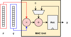
(a) Atomic MAC Unit

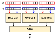
(b) Multi-Staged Accumulation

Figure 2: We visualize (a) an atomic MAC unit and (b) parallelized multi-staged accumulation.

4 Experiments

Models & Datasets. Our experiments consider two fundamental deep learning tasks: image classification and autoregressive language generation. For image classification, we evaluate the top-1 test accuracy of MobileNetV2 [51], ResNet18 [52], and ViT-B-32 [53] on the ImageNet dataset [15] using the pre-trained models made publicly available by the TorchVision library [54]. For language generation, we evaluate the perplexity (PPL) of OPT-125M [20], Pythia-160M [18], and GPT2 [55] on the WikiText2 dataset [16] using the pre-trained models made publicly available by the HuggingFace libraries [56, 57]. Finally, we evaluate multi-staged accumulation on the Pythia model suite [18].

Quantization Design Space. We constrain our quantization design space to uniform-precision models such that every hidden layer has the same weight, activation, and accumulator bit width, respectively denoted as $M$, $N$, and $P$. We consider 3- to 8-bit integers for both weights and activations, unlike [17] and [42], which focused on weight-only quantization. Rather than evaluating each combination of $M$ and $N$, we restrict ourselves to configurations where $N\geq M$ to reduce the cost of experimentation as such configurations tend to dominate the Pareto frontiers [13]. We implement our methods in PyTorch [58] using the Brevitas quantization library [59]. We include all hyperparameter details in Appendix C. All models are quantized using a single AMD MI210 GPU with 64 GB of memory.

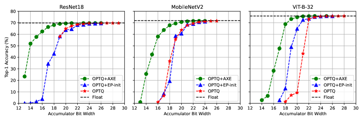
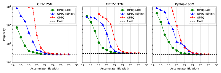
Figure 3: When applied to OPTQ [17], our framework (green circles) significantly improves the trade-off between accumulator bit width and model accuracy when compared to EP-init [13] (blue triangles) and naïve bit width manipulation (red stars) on image classification models evaluated on ImageNet [15] (top) and language generation models evaluated on WikiText2 [16] (bottom).

4.1 Optimizing for Accumulator Constraints

Following [12] and [13], we first consider the scenario in which QNNs are optimized for accumulator-constrained processors. However, unlike prior work, we focus our analysis on the PTQ setting. As discussed in Section 2.3, one could heuristically manipulate the $M$ and $N$ according to the data type bound derived in [12]; however, the quantization design space ultimately limits the minimum attainable accumulator bit width. To the best of our knowledge, Euclidean projection-based initialization (EP-init) [13] serves as the best alternative to this bit width manipulation approach in the PTQ setting (see Section 2.3). Therefore, we use EP-init and naïve bit width manipulation as our baselines.

In Figures 1 and 3, we use Pareto frontiers to visually characterize the trade-off between accumulator bit width and model accuracy for both GPFQ and OPTQ, respectively. For each model and each PTQ algorithm, the Pareto frontier shows the best model accuracy observed for a target accumulator bit width $P$ when varying $M$ and $N$ within our design space, with the 32-bit floating-point model accuracy provided for reference. We provide a detailed breakdown of each Pareto frontier in Appendix D, where we report the accuracy of each Pareto-dominant model, their weight and activation bit widths, and resulting unstructured unstructured weight sparsity. We observe similar trends as reported in [13]; the Pareto-optimal activation bit width $N$ decreases as $P$ is reduced, and the unstructured weight sparsity conversely increases. This suggests that our accumulator-aware boundary constraints obey similar mechanics as the $\ell_{1}$-norm constraints of A2Q [12] and A2Q+ [13], as our theoretical justification predicts (see Section 3.3). Recall that accumulator-aware quantization requires both the weights and activations to be quantized (see Section 3.2); therefore, this is not a direct comparison against the original GPFQ and OPTQ proposals, which only quantized weights.

4.2 Low-Precision Accumulation for Large Language Models

As discussed in [13], the $\ell_{1}$-norm of an unconstrained weight vector inherently grows as its dimensionality increases. This suggests that accumulator-aware quantization scales well to strictly deeper neural architectures since the constraints tighten with width rather than depth; experimental results on the ResNet family support this hypothesis [13]. However, this also suggests that accumulator-aware quantization scales poorly in neural network families that grow in width, as is the case in transformer architectures [20, 18]. Thus, to scale our accumulator-aware PTQ framework to billion-parameter language models, we turn to our multi-stage accumulation variant of AXE (see Section 3.3). Note that this scenario has implications for accelerating inference via software-based compute tiling [60] and hardware-based datapath optimizations [61]. In these examples, one assumes the partial sums of a dot product are concurrently computed in fixed-length tiles of size $T$, which can effectively be interpreted as smaller dot products within our framework. Thus, our goal in this setting is to maximize model accuracy for a target inner accumulator bit width $P_{I}$ that is assumed to be universal across all tiles. In such a setting, our accumulator width is fixed even as models grow wider.

Rather than exploring the full quantization design space, we focus on 4-bit weights and 8-bit activations (W4A8) to maximize utility across platforms with a reasonable number of experiments, as prior studies have suggested this configuration is generally useful [25, 32]. We evaluate AXE on top of both GPFQ and OPTQ using tiles of 64 or 128 elements under 16-bit accumulator constraints (note that $P_{I}^{*}=20$ when $T=128$ for W4A8 via Eq. 3). For each model, we provide the perplexity of both the unconstrained baseline algorithm (e.g., GPFQ or OPTQ with activation quantization) and the original 32-bit floating-point model. We report our results in Table 1. We find that the peak memory utilization of GPFQ precludes its evaluation on billion-parameter LLMs. Thus, we introduce a functionality equivalent memory-efficient reformulation to enable the algorithm to scale to larger models (see Appendix B).

We observe that, as model size increases, the quality of the accumulator-constrained models approaches that of the unconstrained baselines. Under the A2Q scaling hypothesis, this suggests the narrowing accuracy gap is in part because model capacity is growing without tightening the constraints since $T$ is held constant even as $K$ increases. In Appendix C.2, we provide an ablation study targeting a monolithic 16-bit accumulator (i.e., $P_{O}=16$). There, we show the accuracy gap conversely increases as $K$ increases, confirming that fixing $P_{I}$ improves scaling.

Table 1: We evaluate AXE using Pythia models quantized to W4A8 for 16-bit accumulation. For each algorithm, we compare against the unconstrained baseline (Base) and evaluate $T\in\{64,128\}$. We use our memory-efficient GPFQ formulation, which is functionally equivalent to the standard formulation (see Appendix B).

Algorithm		70M (Float: 45.2)	160M (Float: 26.7)	410M (Float: 15.9)	1B (Float: 13.2)	1.4B (Float: 11.8)	2.8B (Float: 10.2)	6.9B (Float: 9.2)
GPFQ*	Base	61.7	40.1	23.0	14.7	15.7	13.3	14.2
	64x16b	61.5	39.8	22.8	14.7	15.7	13.2	14.2
	128x16b	81.9	47.1	25.9	15.4	16.8	14.3	15.2
OPTQ	Base	65.4	46.6	28.9	14.7	15.7	17.3	13.5
	64x16b	66.4	47.8	29.3	14.8	15.5	17.4	16.2
	128x16b	201.4	131.8	60.7	16.2	18.6	16.6	16.2

5 Discussion and Conclusions

As neural networks continue to increase in size, and their weights and activations are increasingly being represented with fewer bits, we anticipate the accumulator to play a larger role in hardware-software co-design (see Section 2.2). While prior work on accumulator-aware quantization has been limited to the quantization-aware training (QAT) setting (see Section 2.3), ours marks the first to extend accumulator-awareness to the post-training quantization (PTQ) setting. To do so, we introduce AXE—a practical low-overhead framework of accumulator-aware extensions designed to endow overflow avoidance guarantees to any layer-wise PTQ algorithm that greedily assign bits element-by-element, provided the base algorithm is also amenable to activation quantization. We demonstrate the flexibility of AXE by presenting accumulator-aware variants of GPFQ [14] and OPTQ [17] with principled overflow avoidance guarantees. Furthermore, unlike prior accumulator-aware quantization methods, which assume a monolithic accumulator, we generalize AXE to support multi-stage accumulation for the first time. Our experiments are designed to investigate two research questions: (1) does AXE fundamentally improve the trade-off between accumulator bit width and model accuracy? and (2) can multi-stage accumulation extend the A2Q scaling hypothesis to large language models (LLMs)?

Our experiments in Section 4.1 show that AXE significantly improves the trade-off between accumulator bit width and model accuracy when compared to existing baselines. This has a direct application to hardware-software co-design, where QNNs are optimized for accumulator-constrained processors, and has implications for accelerating inference on general-purpose platforms [9, 34], reducing the computational overhead of encrypted computations [39, 40], and improving the fault tolerance of embedded deep learning applications [62, 63]. In these examples, one maximizes model accuracy for a known target accumulator bit width, and the chosen PTQ method must be able to guarantee overflow avoidance during inference. As has been shown before in the QAT setting [12, 13], exposing control over the accumulator bit width allows one to reduce $P$ further than what is attainable via naïve bit width manipulations while also maintaining model accuracy. Moreover, we observe that AXE universally yields marked improvement over EP-init across both models and datasets, establishing a new state-of-the-art for accumulator-aware quantization in the PTQ setting. Although EP-init and AXE are both derived from the same convex optimization problem (see Eq. 15), EP-init is a vector projection that is applied after quantization and relies on the round-to-zero rounding function to ensure the $\ell_{1}$-norm constraints are respected. Previous reports had suspected EP-init is limited by this reliance on round-to-zero [12, 13]; we provide an ablation study in Appendix C.2 that supports this hypothesis but also suggests error correction is critical. For GPFQ, we observe error correction to be more important than round-to-nearest, but we observe the opposite for OPTQ, although a more exhaustive analysis in future work may uncover more insights.

Our experiments in Section 4.2 show that our generalized multi-stage accumulation enables the A2Q scaling hypothesis to extend to LLMs in the Pythia model suite. However, while we observe that the perplexity gap shrinks between the constrained and unconstrained quantized models, we also observe that the perplexity gap between the quantized models and their 32-bit floating-point counterparts begins to increase as the model size increases. We note that this is consistent with the findings of Li et al. [25], who conclude that while larger models tend to have a higher tolerance for weight quantization, they also tend to have a lower tolerance for activation quantization. Thus, there exists two diametrically opposing trends in superposition. For the Pythia model suite, we observe Pythia-1B to be the equilibrium point where the costs of weight and activation quantization are balanced. While it is orthogonal to the scope of this study, we expect the emerging rotation-based quantization schemes (e.g., QuaRot [64], SpinQuant [65]) to impact this equilibrium point and reduce the gap between accumulator-constrained quantized models and their 32-bit floating-point counterparts. We leave such investigations for future work.

Appendix A Psuedo-code for Accumulator-Aware Variants of GPFQ and OPTQ

We present the pseudo-code for our accumulator-aware variants of GPFQ [14] and OPTQ [17] in Algorithms 1 and 2, respectively, where we define $\Psi_{\bm{a},\bm{b}}(\bm{v})$ to denote the clipping function applied elementwise so that $(\Psi_{\bm{a},\bm{b}}(\bm{v}))_{j}=\Psi_{{a_{j}},{b_{j}}}({v_{j}})$. We direct the reader to Section 3 for theoretical justification for these algorithms.

Algorithm 1 Accumulator-Aware GPFQ. Our accumulator-aware GPFQ variant [14] quantizes $\bm{W}$ to $M$ bits given input activations $\bm{X}$ and their $N$-bit quantized counterparts $\tilde{\bm{X}}$. Note that $\bm{W}_{i},\bm{V}_{i}\in\mathbb{R}^{C}$, $\bm{Q}_{i}\in\mathcal{A}^{C}_{M}$, $\bm{X}_{i}\in\mathbb{R}^{D}$, and $\bm{\tilde{X}}_{i}\in\mathcal{A}^{D}_{N}$, all interpreted as row vectors.

1:$\bm{W}\in\mathbb{R}^{K\times C}$, $\bm{X}\in\mathbb{R}^{K\times D}$, $\tilde{\bm{X}}\in\mathcal{A}^{K\times D}_{N}$

2:$\bm{Q}\leftarrow 0\in\mathcal{A}^{K\times C}_{M}$. // Quantized output

3:$\bm{U}\leftarrow 0\in\mathbb{R}^{D\times C}$ // Per-sample quantization error

4:$\bm{a}\leftarrow A\in\mathbb{R}^{C}$, $\bm{b}\leftarrow B\in\mathbb{R}^{C}$ // Initialize running sums

5:$\lambda\leftarrow\textrm{deriveThreshold}(\bm{W})$ // Derive per-channel Lagrangian thresholds

6:for $i=1,...,K$ do

7:     $\bm{V}_{i}\leftarrow\bm{W}_{i}\frac{\langle\tilde{\bm{X}}_{i},\bm{X}_{i}\rangle}{\|\tilde{\bm{X}}_{i}\|^{2}_{2}}+\frac{\tilde{\bm{X}}_{i}\bm{U}}{\|\tilde{\bm{X}}_{i}\|^{2}_{2}}$ // Adjust for quantization error

8:     $\bm{V}_{i}\leftarrow\Psi_{\bm{a},\bm{b}}\circ\Pi_{\lambda}(\bm{V}_{i})$ // Accumulator-aware projection & clipping

9:     $\bm{Q}_{i}\leftarrow\mathcal{Q}(\bm{V}_{i})$ // Quantize weight

10:     $\bm{a}\leftarrow\bm{a}-\bm{Q}_{i}\odot\mathbbm{1}_{\bm{Q}_{i}\geq 0}$ // Update positive range

11:     $\bm{b}\leftarrow\bm{b}-\bm{Q}_{i}\odot\mathbbm{1}_{\bm{Q}_{i}\leq 0}$ // Update negative range

12:     $\bm{U}\leftarrow\bm{U}+\bm{X}_{i}^{T}\bm{W}_{i}-\tilde{\bm{X}}_{i}^{T}\bm{Q}_{i}$ // Update quantization error

13:end for

14:return $\bm{Q}$

Algorithm 2 Accumulator-Aware OPTQ. Our accumulator-aware OPTQ variant [17] quantizes $\bm{W}$ to $M$ bits given $\bm{H}^{-1}=\textrm{Cholesky}((2\tilde{\bm{X}}\tilde{\bm{X}}^{T}+\eta\bm{I})^{-1})$, where $\eta$ is a small dampening factor to avoid numerical issues. Following [17], we set $\eta$ to be $1\%$ of the average diagonal value. Note that $\bm{W}_{i},\bm{V}_{i}\in\mathbb{R}^{C}$ and $\bm{Q}_{i}\in\mathcal{A}^{C}_{M}$, all interpreted as row vectors.

1:$\bm{W}\in\mathbb{R}^{K\times C}$, $\bm{H}^{-1}\in\mathbb{R}^{K\times K}$

2:$\bm{Q}\leftarrow 0\in\mathcal{A}^{K\times C}_{M}$ // Quantized output

3:$\bm{E}\leftarrow 0\in\mathbb{R}^{C}$ // Per-channel quantization errors

4:$\bm{a}\leftarrow A\in\mathbb{R}^{C}$, $\bm{b}\leftarrow B\in\mathbb{R}^{C}$ // Initialize running sums

5:$\lambda\leftarrow\textrm{deriveThreshold}(\bm{W})$ // Derive per-channel Lagrangian thresholds

6:for $i=1,...,K$ do

7:     $\bm{V}_{i}\leftarrow\Psi_{\bm{a},\bm{b}}\circ\Pi_{\lambda}(\bm{W}_{i})$ // Accumulator-aware projection & clipping

8:     $\bm{Q}_{i}\leftarrow\mathcal{Q}(\bm{V}_{i})$ // Quantize processed weight

9:     $\bm{E}\leftarrow(\bm{W}_{i}-\bm{Q}_{i})/\bm{H}^{-1}_{i,i}$ // Calculate quantization error

10:     $\bm{W}_{i:K}\leftarrow\bm{W}_{i:K}-\bm{E}\cdot\bm{H}^{-1}_{i,i:K}$ // Update weights

11:     $\bm{a}\leftarrow\bm{a}-\bm{Q}_{i}\odot\mathbbm{1}_{\bm{Q}_{i}\geq 0}$ // Update positive range

12:     $\bm{b}\leftarrow\bm{b}-\bm{Q}_{i}\odot\mathbbm{1}_{\bm{Q}_{i}\leq 0}$ // Update negative range

13:end for

14:return $\bm{Q}$

Appendix B Memory-Efficient GPFQ

As discussed in Section 3.2, GPFQ approaches the standard quantization problem by traversing the neural network graph to sequentially quantize each element in each layer while iteratively correcting for quantization error. The derived iteration rule is formalized by Eqs. 11 and 12. In this standard formulation, the $i$-th quantized weight $q_{i}$ depends on the inner product

$$\langle\tilde{\bm{X}}^{(l)}_{i},\bm{u}^{(l)}_{i-1}+w^{(l)}_{i}\bm{X}^{(l)}_{i}\rangle$$

where $\bm{X}^{(l)}_{i},\bm{\tilde{X}}^{(l)}_{i}\in\mathbb{R}^{D}$ are samples for the $i$-th neuron of the inputs to layer $l$, and $\bm{u}_{i-1}^{(l)}\in\mathbb{R}^{D}$ is the running error from quantizing the first $i-1$ weights. Thus, at layer $l$, GPFQ requires collecting and storing $2D$ samples for the $K_{l}$ input neurons, and updating the running quantization error for each sample for the $C_{l}$ output neurons. This implies poor scaling to larger models and larger calibration sets as the memory requirements are $O(D\times(2K_{l}+C_{l}))$. Indeed, assuming 128 samples with a sequence length of 2048 at 32-bit precision, Pythia-6.9B [18] requires a peak memory usage of roughly 30 GB at the first FFN layer excluding pre-trained weights. We set out to reduce this overhead.

We start with the observation that OPTQ is far more memory efficient. OPTQ uses the Hessian proxy $2\bm{X}\bm{X}^{T}$, which can be efficiently computed one sample at a time and stored as a $K_{l}\times K_{l}$ square matrix, an $O(K_{l}\times K_{l})$ memory requirement that is $36\times$ less than GPFQ for Pythia-6.9B. Thus, we reformulate GPFQ to use square matrices via mathematical manipulation of singular value decompositions. We present the following theorem:

Theorem B.1.

Let $\bm{H}=\left(\tilde{\bm{X}}\tilde{\bm{X}}^{T}\right)^{1/2}$ and $\bm{G}=\bm{X}\tilde{\bm{X}}^{T}$. For pre-trained weights $\bm{W}\in\mathbb{R}^{K\times C}$, quantization alphabet $\mathcal{A}$, and GPFQ function of the form of Algorithm 1, it follows that:

$$\textrm{GPFQ}(\bm{W},\bm{X},\bm{\tilde{X}},\mathcal{A})=\textrm{GPFQ}(\bm{W},\bm{G}\bm{H}^{-1},\bm{H},\mathcal{A})$$ (23)

Proof.

According to the iteration steps in Algorithm 1, it suffices to show that the argument of quantizer $\mathcal{Q}$ is unchanged after substituting $\bm{X}_{i}$, $\tilde{\bm{X}}_{i}$ with $(\bm{G}\bm{H}^{-1})_{i}$ and $\bm{H}_{i}$ respectively. Specifically, at the $i$-th iteration of $\textrm{GPFQ}(\bm{W},\bm{G}\bm{H}^{-1},\bm{H},\mathcal{A})$, we have

$$\bm{V}_{i}\leftarrow\bm{W}_{i}\frac{\langle\bm{H}_{i},(\bm{G}\bm{H}^{-1})_{i}\rangle}{\|\bm{H}_{i}\|^{2}_{2}}+\frac{\bm{H}_{i}\bm{U}_{i-1}}{\|\bm{H}_{i}\|^{2}_{2}}$$ (24)

where the quantization error is given by

$$\bm{U}_{i-1}=\sum_{j=1}^{i-1}(\bm{G}\bm{H}^{-1})_{j}^{T}\bm{W}_{j}-\bm{H}_{j}^{T}\bm{Q}_{j}.$$ (25)

Let $\bm{e}_{i}\in\mathbb{R}^{K}$ denote the vector with a $1$ in the $i$-th coordinate and $0$’s elsewhere. It follows from $\bm{H}=\left(\tilde{\bm{X}}\tilde{\bm{X}}^{T}\right)^{1/2}$ and $\bm{G}=\bm{X}\tilde{\bm{X}}^{T}$ that

$$\|\bm{H}_{i}\|_{2}^{2}=\|\bm{e}_{i}^{T}\bm{H}\|_{2}^{2}=\bm{e}_{i}^{T}\bm{H}^{2}\bm{e}_{i}=\bm{e}_{i}^{T}\tilde{\bm{X}}\tilde{\bm{X}}^{T}\bm{e}_{i}=\|\tilde{\bm{X}}_{i}\|_{2}^{2},$$

$$\bm{H}_{i}(\bm{G}\bm{H}^{-1})_{j}^{T}=\bm{e}_{i}^{T}\bm{H}(\bm{e}_{j}^{T}\bm{G}\bm{H}^{-1})^{T}=\bm{e}_{i}^{T}\bm{G}^{T}\bm{e}_{j}=\bm{e}_{i}^{T}\tilde{\bm{X}}\bm{X}^{T}\bm{e}_{j}=\tilde{\bm{X}}_{i}\bm{X}_{j}^{T},$$

and

$$\bm{H}_{i}\bm{H}_{j}^{T}=\bm{e}_{i}^{T}\bm{H}(\bm{e}_{j}^{T}\bm{H})^{T}=\bm{e}_{i}^{T}\bm{H}^{2}\bm{e}_{j}=\bm{e}_{i}^{T}\tilde{\bm{X}}\tilde{\bm{X}}^{T}\bm{e}_{j}=\tilde{\bm{X}}_{i}\tilde{\bm{X}}_{j}^{T}.$$

Plugging above identities into (24) and (25), we obtain

$$\bm{V}_{i}\leftarrow\bm{W}_{i}\frac{\langle\tilde{\bm{X}}_{i},\bm{X}_{i}\rangle}{\|\tilde{\bm{X}}_{i}\|^{2}_{2}}+\frac{\tilde{\bm{X}}_{i}\hat{\bm{U}}_{i-1}}{\|\tilde{\bm{X}}_{i}\|^{2}_{2}}$$ (26)

with $\hat{\bm{U}}_{i-1}=\sum_{j=1}^{i-1}\bm{X}_{j}^{T}\bm{W}_{j}-\tilde{\bm{X}}_{j}^{T}\bm{Q}_{j}$. Since $\bm{V}_{i}$ in (26) is identical with the $i$-th quantization argument in $\textrm{GPFQ}(\bm{W},\bm{X},\bm{\tilde{X}},\mathcal{A})$, both algorithms derive the same quantized weights $\bm{Q}_{i}=\mathcal{Q}(\bm{V}_{i})$. This completes the proof. ∎

At layer $l$, this memory-efficient GPFQ formulation requires collecting and storing $G$, $H$, and $U$, which are each $K_{l}\times K_{l}$ matrices, reducing to an $O(K_{l}\times K_{l})$ memory requirement that is $12\times$ less than the standard GPFQ formulation for Pythia-6.9B. We leverage this functionally equivalent formulation for our LLM evaluations in Section 4.2.

Appendix C Experimental Details & Ablations

C.1 Hyperparameters & Quantization Schemes

Below, we provide a detailed description of the quantization schemes and the specific hyperparameters used in our experiments. As discussed in Section 4, we consider pre-trained image classification and language models that are respectively made publicly available via the TorchVision [54] and HuggingFace [56] libraries. All models are quantized via the Brevitas [59] quantization library using a single AMD MI210 GPU with 64 GB of memory.

Image Classification Models. We leverage the unmodified implementations of ResNet18 [52], MobileNetV2 [51], and ViT-B-32 [53] as well as their floating-point checkpoints pre-trained on ImageNet [15]. We use drop-in replacements for all convolution and linear layers in each network while universally holding the input and output layers to 8-bit weights and activations, as is common practice [3]. We build our calibration set from the ImageNet training dataset by randomly sampling one image per class, resulting in a calibration set of 1000 images.

Large Language Models (LLMs). We leverage the unmodified implementations of the various LLMs discussed in Section 4 as provided by HuggingFace [56], as well as their pre-trained floating-point checkpoints and datasets [57]. We use drop-in replacements for all linear layers in the networks except the embedding layer or final prediction head, leaving them at 32-bit floating-point. As is common practice [17], we build our calibration set using 128 samples randomly selected from the WikiText2 dataset [16] without replacement using a fixed sequence length of 2048 tokens for all models except GPT2 [55], which is restricted to a maximum sequence length of 1024 by the library.

Quantization Scheme. As discussed in Section 2, we adopt the standard uniform integer quantizer parameterized by scaling factor $s$ and zero-point $z$. We quantize activations asymmetrically, tuning $z$ to the lowest 99-th percentile based on the calibration data. While AXE is not reliant on symmetric weight quantization, we eliminate zero-points in all weight quantizers such that $z=0$, as is common practice so as to avoid computational overhead of cross-terms [2, 44]. Throughout our experiments, we adopt 32-bit floating-point scaling factors that take the form of Eq. 27, where $\max(\bm{w})$ is calculated per-channel for the weights and per-tensor for the activations quantized to $b$ bits.

$$s=\frac{\max(\bm{w})}{2^{b-1}-1}$$ (27)

Quantization Process. To quantize our models, we first load the pre-trained checkpoint and merge batch normalization layers if they exist, then we apply graph equalization before calibrating the scaling factors and zero-points. We apply graph equalization as proposed by Nagel et al. [26] for image classification models (i.e., weight equalization) and graph equalization as proposed by Xiao et al. [24] for language models (i.e., SmoothQuant), the only difference being the optimization criteria; weight equalization is derived to maximize the per-channel precision while SmoothQuant is derived to migrate quantization difficulty from the activations to the weights. We then apply either GPFQ [14] or OPTQ [17] (with or without AXE) before finally applying bias correction [26]. When sequentially quantizing weights element-by-element, we do so in descending order according to the diagonal value of the Hessian proxy ($2\bm{X}\bm{X}^{T}$ by our notation in Section 2), which was originally implemented in [66] and reported to yield superior results in [19, 28]. When evaluating EP-init in the PTQ setting, we do so after OPTQ or GPFQ but before bias correction. Because bias correction does not adjust weight values, this allows us to at least perform some form of error correction with EP-init while still ensuring guaranteed overflow avoidance.

C.2 Ablation Studies

Impact of error correction, choice of rounding function, and soft thresholding. Previous reports had suspected EP-init is limited by its reliance on the round-to-zero (RTZ) rounding function [12, 13], which has been shown to be a poor choice [67]. AXE removes this reliance and also enables greedy error correction. We design an ablation study to isolate the impact of RTZ and error correction. We quantize OPT-125M [20] and Pythia-160M [18] to 4-bit weights and 8-bit activations while targeting 20-bit accumulation since our Pareto front shows this configuration to be both reasonable and challenging. We evaluate AXE with round-to-zero (AXE-RTZ) and AXE with round-to-nearest (AXE-RTN). We report the results in Table 2. We interpret the gap between EP-init and AXE-RTZ as the benefit of error correction, and the gap between AXE-RTZ and AXE-RTN as the benefit of rounding function. We observe that error correction has a greater impact than rounding function selection for GPFQ, but we observe the opposite for OPTQ. Finally, we evaluate AXE with our hard constraint only (AXE-HCO) to isolate the impact of our soft constraint, which is not necessary for guaranteeing overflow avoidance. We interpret the gap between AXE-RTN and AXE-HCO as the impact of our soft constraint, which consistently provides improved or maintained performance.

Table 2: We evaluate round-to-nearest (RTN) and round-to-zero (RTZ) within our AXE framework to directly compare against EP-init. We also evaluate AXE with our hard constraint only (HCO) to isolate the impact of our soft constraint. All models are quantized to W4A8 while targeting a 20-bit accumulator.

Algorithm	Model	EP-init	AXE-RTZ	AXE-RTN	AXE-HCO
GPFQ	OPT-125M	8828.3	165.2	31.9	31.9
	Pythia-160M	2500.2	211.0	43.0	49.2
OPTQ	OPT-125M	998.6	539.3	37.1	70.0
	Pythia-160M	4524.4	1798.7	84.9	194.8

Multi-stage vs. monolithic accumulation. In Section 4.2, we analyze how our accumulator constraints scale to increasingly large language models within the Pythia model suite [18]. There, we discuss our observation that, as model size increases, the quality of the accumulator-constrained models approaches that of the unconstrained baselines for both GPFQ and OPTQ. Under the A2Q scaling hypothesis, this suggests the narrowing accuracy gap is in part because model capacity is growing without tightening the constraints. To verify this, we perform an ablation study targeting a monolithic 16-bit accumulator (i.e., $P_{0}=16$). We quantize all Pythia models up to Pythia-1B, which we had observed to be the equilibrium point between weight and activation quantization scaling trends (see Section 5). Not only do we observe significant instability, we also observe a $7.4\times$ regression in perplexity between Pythia-70M and Pythia-1B, confirming that fixing $P_{I}$ improves scaling as models grow wider.

Table 3: We evaluate AXE using Pythia models quantized to W4A8 when targeting a monolithic 16-bit accumulator (i.e., $P_{O}=16$). Note that this is in direct contrast with Table 1, which targets multi-stage accumulation.

Algorithm	70M (Float: 45.2)	160M (Float: 26.7)	410M (Float: 15.9)	1B (Float: 13.2)
GPFQ	4397	7135	10496	32601
OPTQ	2438	4439	9759	34387

Appendix D Pareto Frontier Details

We provide the detailed Pareto frontiers visualized in Figures 1 and 3 for GPFQ and OPTQ, respectively. For each model, we report the model accuracy, quantization configuration, and resulting unstructured weight sparsity.

D.1 GPFQ

Table 4: Image Classification (GPFQ). We provide the top-1 test accuracy and quantization configuration of the Pareto-optimal models that form the frontiers visualized in Figure 1. Note that $M$ and $N$ respectively denote the weight and activation bit widths.

Model	P	GPFQ			GPFQ+EP-init			GPFQ+AXE
		Top-1	$(M,N)$	Sparsity	Top-1	$(M,N)$	Sparsity	Top-1	$(M,N)$	Sparsity
ResNet18 (Float: 69.8)	14	-	-	-	0.2	(3,3)	83.5	50.8	(3,3)	56.9
	15	-	-	-	1.0	(3,3)	74.3	58.1	(3,4)	58.6
	16	-	-	-	10.8	(3,3)	62.3	63.3	(4,4)	40.4
	17	-	-	-	43.9	(4,4)	57.2	66.5	(4,4)	29.9
	18	-	-	-	59.6	(4,4)	43.5	67.9	(4,5)	30.7
	19	54.5	(3,3)	47.4	62.0	(4,5)	44.1	68.9	(5,5)	16.7
	20	62.0	(3,4)	49.5	67.3	(5,5)	27.6	69.3	(5,6)	16.8
	21	66.5	(4,4)	29.8	67.9	(5,6)	27.8	69.5	(6,6)	8.7
	22	67.9	(4,5)	30.5	69.1	(6,6)	15.7	69.7	(6,7)	8.7
	32	69.8	(8,8)	2.3	69.7	(8,8)	4.4	69.8	(8,8)	2.3
MobileNetV2 (Float: 71.9)	14	-	-	-	-	-	-	5.2	(4,4)	17.6
	15	-	-	-	-	-	-	35.1	(4,5)	16.7
	16	0.1	(3,3)	33.8	0.3	(4,4)	26.5	51.4	(4,6)	16.6
	17	0.9	(3,4)	30.2	18.2	(5,5)	16.7	61.7	(5,6)	9.6
	18	6.4	(3,5)	28.8	49.0	(5,6)	16.8	67.2	(5,7)	9.7
	19	37.6	(4,5)	15.2	60.9	(6,6)	10.1	68.3	(5,7)	7.9
	20	54.1	(4,6)	14.9	66.7	(6,7)	10.3	69.9	(6,8)	5.9
	21	64.3	(5,6)	8.0	68.2	(7,7)	6.5	70.6	(7,8)	4.2
	22	68.3	(5,7)	7.9	69.7	(7,8)	6.4	70.7	(7,8)	2.3
	32	71.0	(8,8)	1.4	70.8	(8,8)	2.7	71.0	(8,8)	1.4
ViT-B-32 (Float: 75.9)	16	-	-	-	0.1	(3,3)	89.0	64.1	(3,5)	46.9
	17	-	-	-	0.4	(3,4)	67.5	69.1	(4,5)	31.3
	18	0.2	(3,3)	51.2	6.4	(4,5)	47.5	72.9	(3,7)	46.0
	19	35.7	(3,4)	47.1	41.7	(4,5)	43.4	75.1	(4,7)	30.0
	20	64.9	(3,5)	45.0	66.6	(5,5)	27.8	75.3	(4,8)	29.2
	21	70.0	(4,5)	28.7	69.1	(4,7)	40.2	75.7	(5,8)	18.8
	22	73.2	(3,7)	43.6	72.7	(5,8)	27.3	75.8	(6,8)	12.3
	23	75.2	(4,7)	27.4	75.1	(6,8)	17.2	75.8	(6,8)	9.3
	24	75.6	(5,7)	16.5	75.6	(6,8)	15.1	75.9	(8,8)	6.3
	32	75.9	(8,8)	5.4	75.9	(8,8)	5.2	75.9	(8,8)	5.4

Table 5: Language Generation (GPFQ). We provide the test perplexity (PPL) and quantization configuration of the Pareto-optimal models that form the frontiers visualized in Figure 1. Note that $M$ and $N$ respectively denote the weight and activation bit widths.

Model	P	GPFQ			GPFQ+EP-init			GPFQ+AXE
		PPL	$(M,N)$	Sparsity	PPL	$(M,N)$	Sparsity	PPL	$(M,N)$	Sparsity
OPT-125M (Float: 27.7)	16	-	-	-	9148.8	(3,4)	76.5	249.8	(3,6)	55.6
	17	-	-	-	7624.6	(3,4)	72.7	91.2	(4,6)	37.9
	18	11007.2	(3,3)	58.3	7471.2	(3,5)	75.5	41.8	(4,6)	27.8
	19	9567.6	(3,4)	54.5	1059.3	(5,6)	39.1	32.3	(4,7)	27.0
	20	874.4	(3,5)	50.5	86.1	(5,6)	29.8	29.3	(5,7)	15.7
	21	101.0	(3,6)	46.4	42.4	(5,7)	28.1	28.6	(5,8)	15.6
	22	40.5	(4,6)	26.3	30.4	(6,7)	16.0	28.1	(6,8)	9.6
	23	31.8	(4,7)	25.9	29.5	(6,8)	15.9	27.9	(6,8)	8.6
	24	29.0	(5,7)	14.7	28.2	(7,8)	9.5	27.8	(7,8)	5.4
	32	27.8	(8,8)	3.8	27.8	(8,8)	5.3	27.8	(8,8)	3.8
GPT2-137M (Float: 29.9)	16	-	-	-	3345.8	(3,3)	93.2	552.4	(3,6)	55.4
	17	-	-	-	2705.3	(3,6)	75.1	310.1	(3,7)	52.8
	18	3760.3	(3,3)	82.3	1100.5	(4,5)	52.9	134.3	(4,7)	34.9
	19	2782.2	(3,4)	43.9	402.9	(4,6)	47.3	67.5	(4,7)	25.6
	20	742.4	(3,5)	55.3	213.2	(4,7)	44.3	40.4	(4,8)	24.5
	21	356.2	(3,6)	48.8	85.2	(5,7)	24.9	33.2	(5,8)	13.2
	22	189.9	(4,6)	26.4	46.3	(5,8)	23.8	32.1	(6,8)	7.3
	23	65.8	(4,7)	24.7	34.2	(6,8)	13.0	31.8	(6,8)	6.3
	24	39.8	(4,8)	23.8	32.1	(7,8)	7.1	31.5	(7,8)	3.2
	32	31.5	(8,8)	1.6	31.6	(8,8)	3.2	31.5	(8,8)	1.6
Pythia-160M (Float: 26.7)	16	-	-	-	4501.1	(3,4)	76.8	386.0	(3,6)	53.2
	17	-	-	-	3095.1	(3,5)	72.5	198.6	(3,6)	46.3
	18	9887.1	(3,3)	49.4	1070.2	(4,5)	46.7	74.5	(4,6)	25.1
	19	1946.8	(3,4)	49.8	391.7	(4,6)	42.9	46.2	(4,7)	24.4
	20	456.2	(3,5)	47.8	117.5	(5,6)	23.6	34.6	(5,7)	13.3
	21	198.3	(3,6)	45.1	78.5	(5,7)	23.4	32.4	(5,8)	13.3
	22	69.6	(4,6)	23.5	48.6	(5,7)	21.2	30.1	(6,8)	7.8
	23	44.4	(4,7)	22.6	37.2	(6,8)	13.0	28.2	(6,8)	5.5
	24	33.2	(5,7)	11.3	31.8	(7,8)	7.4	27.6	(7,8)	2.8
	32	27.4	(8,8)	1.4	27.5	(8,8)	2.7	27.4	(8,8)	1.4

D.2 OPTQ

Table 6: Image Classification (OPTQ). We provide the top-1 test accuracy and quantization configuration of the Pareto-optimal models that form the frontiers visualized in Figure 3. Note that $M$ and $N$ respectively denote the weight and activation bit widths.

Model	P	OPTQ			OPTQ+EP-init			OPTQ+AXE
		Top-1	$(M,N)$	Sparsity	Top-1	$(M,N)$	Sparsity	Top-1	$(M,N)$	Sparsity
ResNet18 (Float: 69.8)	14	-	-	-	0.1	(3,3)	82.6	51.9	(3,3)	58.9
	15	-	-	-	1.5	(3,3)	71.6	57.7	(3,4)	59.9
	16	-	-	-	3.8	(3,4)	72.0	62.5	(4,4)	39.1
	17	-	-	-	34.4	(4,4)	55.6	66.4	(4,4)	32.0
	18	-	-	-	43.1	(4,4)	49.9	68.1	(4,5)	32.0
	19	58.0	(3,3)	54.1	58.2	(5,5)	37.7	69.1	(5,5)	17.1
	20	64.9	(3,4)	54.1	63.7	(5,5)	30.3	69.4	(5,6)	17.0
	21	67.2	(4,4)	31.9	64.5	(6,6)	25.0	69.5	(6,6)	8.7
	22	68.6	(4,5)	31.9	68.2	(6,6)	16.9	69.6	(6,7)	8.7
	32	69.7	(8,8)	2.3	69.7	(8,8)	4.4	69.7	(8,8)	2.3
MobileNetV2 (Float: 71.9)	14	-	-	-	-	-	-	25.2	(4,4)	16.2
	15	-	-	-	-	-	-	42.5	(4,5)	16.4
	16	1.0	(3,3)	26.6	0.1	(4,4)	32.4	58.0	(5,5)	9.5
	17	6.6	(3,4)	26.5	8.4	(5,5)	17.0	63.7	(5,5)	8.0
	18	36.6	(4,4)	28.8	19.4	(5,6)	17.2	67.8	(5,6)	7.9
	19	55.6	(4,5)	15.2	58.5	(6,6)	10.2	69.4	(5,7)	8.0
	20	63.7	(5,5)	14.9	60.6	(6,7)	10.2	70.7	(6,7)	4.2
	21	67.8	(5,6)	7.9	68.5	(7,7)	6.5	71.2	(7,7)	2.4
	22	69.4	(5,7)	7.9	69.0	(7,8)	6.5	71.5	(7,8)	2.4
	32	71.6	(8,8)	1.4	71.1	(8,8)	2.9	71.6	(8,8)	1.4
ViT-B-32 (Float: 75.9)	16	-	-	-	0.1	(3,3)	89.0	28.3	(3,6)	63.2
	17	-	-	-	2.7	(3,5)	66.8	47.4	(3,6)	53.0
	18	1.4	(3,3)	52.5	13.0	(3,6)	65.4	68.8	(3,7)	53.1
	19	7.1	(3,4)	50.8	48.9	(4,6)	48.1	73.3	(3,7)	48.2
	20	10.2	(3,5)	54.1	64.8	(4,7)	47.3	74.8	(4,7)	32.8
	21	47.7	(3,6)	53.0	72.6	(5,7)	33.6	75.6	(4,8)	32.4
	22	73.3	(3,7)	48.2	73.5	(5,8)	33.2	75.7	(6,8)	22.0
	23	74.8	(4,7)	32.8	75.0	(6,8)	23.2	75.9	(6,8)	14.4
	24	75.6	(4,8)	32.4	75.6	(6,8)	21.5	75.9	(8,8)	9.4
	32	75.9	(8,8)	8.6	75.8	(8,8)	10.0	75.9	(8,8)	8.6

Table 7: Language Generation (OPTQ). We provide the test perplexity (PPL) and quantization configuration of the Pareto-optimal models that form the frontiers visualized in Figure 1. Note that $M$ and $N$ respectively denote the weight and activation bit widths.

Model	P	OPTQ			OPTQ+EP-init			OPTQ+AXE
		PPL	$(M,N)$	Sparsity	PPL	$(M,N)$	Sparsity	PPL	$(M,N)$	Sparsity
OPT-125M (Float: 27.7)	16	-	-	-	3333.8	(4,5)	62.2	225.0	(3,6)	52.8
	17	-	-	-	1722.6	(4,5)	53.6	80.2	(3,6)	45.7
	18	9942.5	(3,3)	54.5	409.8	(5,5)	36.1	41.3	(4,6)	26.6
	19	8278.3	(3,4)	47.5	136.0	(5,6)	35,7	35.0	(5,6)	15.1
	20	281.1	(3,5)	45.5	46.9	(5,6)	26.8	31.3	(5,6)	14.2
	21	60.4	(3,6)	44.7	40.1	(5,7)	26.8	29.0	(5,7)	14.2
	22	35.7	(4,6)	25.8	30.3	(6,7)	15.6	28.5	(5,8)	14.2
	23	31.5	(5,6)	14.6	29.7	(6,8)	15.6	28.0	(6,8)	8.6
	24	29.2	(5,7)	14.6	28.1	(7,8)	9.5	27.8	(7,8)	5.4
	32	27.8	(8,8)	2.2	27.8	(8,8)	5.6	27.8	(8,8)	2.2
GPT2-137M (Float: 29.9)	16	-	-	-	2765.6	(4,4)	52.6	1513.6	(4,5)	34.0
	17	-	-	-	2465.0	(4,4)	49.0	496.4	(3,6)	43.4
	18	4140.7	(3,3)	59.3	2465.0	(4,4)	49.0	117.9	(4,6)	24.2
	19	2782.2	(3,4)	43.9	1108.4	(5,6)	34.5	59.9	(4,7)	24.2
	20	2149.8	(4,4)	26.0	361.7	(4,7)	43.6	45.5	(5,7)	13.1
	21	1153.8	(4,5)	24.7	73.1	(5,7)	24.7	37.3	(5,8)	13.2
	22	176.9	(4,6)	24.0	42.7	(5,8)	24.5	33.1	(6,8)	12.2
	23	50.1	(4,7)	23.2	33.5	(6,8)	13.4	32.1	(6,8)	6.2
	24	37.4	(5,7)	12.2	32.0	(7,8)	7.3	31.8	(7,8)	3.1
	32	31.8	(8,8)	1.6	31.7	(8,8)	3.3	31.7	(8,8)	1.6
Pythia-160M (Float: 26.7)	16	-	-	-	6739.6	(4,6)	79.7	1521.2	(3,5)	41.7
	17	-	-	-	5345.7	(4,5)	49.9	311.7	(4,5)	22.9
	18	27098.1	(3,3)	40.5	1372.4	(4,5)	41.1	126.1	(4,6)	23.1
	19	5644.0	(3,4)	40.3	641.2	(4,6)	41.0	61.4	(4,6)	21.3
	20	948.4	(3,5)	40.1	132.9	(5,6)	23.4	43.5	(5,6)	10.9
	21	151.3	(4,5)	21.4	108.5	(5,7)	23.5	32.8	(5,7)	10.9
	22	61.4	(4,6)	21.3	74.1	(5,7)	22.0	30.0	(5,8)	10.9
	23	43.3	(5,6)	10.9	40.4	(6,8)	13.0	28.0	(6,8)	5.5
	24	32.8	(5,7)	10.9	32.1	(7,8)	7.5	27.4	(7,8)	2.7
	32	27.2	(8,8)	1.4	27.6	(8,8)	2.9	27.2	(8,8)	1.4

References

- [1] H. Wu, P. Judd, X. Zhang, M. Isaev, and P. Micikevicius, “Integer quantization for deep learning inference: Principles and empirical evaluation,” arXiv preprint arXiv:2004.09602, 2020.
- [2] M. Nagel, M. Fournarakis, R. A. Amjad, Y. Bondarenko, M. Van Baalen, and T. Blankevoort, “A white paper on neural network quantization,” arXiv preprint arXiv:2106.08295, 2021.
- [3] A. Gholami, S. Kim, Z. Dong, Z. Yao, M. W. Mahoney, and K. Keutzer, “A survey of quantization methods for efficient neural network inference,” in Low-Power Computer Vision, pp. 291–326, Chapman and Hall/CRC, 2022.
- [4] S. Han, X. Liu, H. Mao, J. Pu, A. Pedram, M. A. Horowitz, and W. J. Dally, “EIE: Efficient inference engine on compressed deep neural network,” ACM SIGARCH Computer Architecture News, vol. 44, no. 3, pp. 243–254, 2016.
- [5] V. Sze, Y.-H. Chen, T.-J. Yang, and J. S. Emer, “Efficient processing of deep neural networks: A tutorial and survey,” Proceedings of the IEEE, vol. 105, no. 12, pp. 2295–2329, 2017.
- [6] M. Blott, T. B. Preußer, N. J. Fraser, G. Gambardella, K. O’brien, Y. Umuroglu, M. Leeser, and K. Vissers, “FINN-R: An end-to-end deep-learning framework for fast exploration of quantized neural networks,” ACM Transactions on Reconfigurable Technology and Systems (TRETS), vol. 11, no. 3, pp. 1–23, 2018.
- [7] R. Ni, H.-m. Chu, O. Castañeda, P.-y. Chiang, C. Studer, and T. Goldstein, “Wrapnet: Neural net inference with ultra-low-resolution arithmetic,” arXiv preprint arXiv:2007.13242, 2020.
- [8] B. de Bruin, Z. Zivkovic, and H. Corporaal, “Quantization of deep neural networks for accumulator-constrained processors,” Microprocessors and microsystems, vol. 72, p. 102872, 2020.
- [9] H. Xie, Y. Song, L. Cai, and M. Li, “Overflow aware quantization: Accelerating neural network inference by low-bit multiply-accumulate operations,” in Proceedings of the Twenty-Ninth International Conference on International Joint Conferences on Artificial Intelligence, pp. 868–875, 2021.
- [10] I. Colbert, A. Pappalardo, and J. Petri-Koenig, “Quantized neural networks for low-precision accumulation with guaranteed overflow avoidance,” arXiv preprint arXiv:2301.13376, 2023.
- [11] J. Yang, X. Wang, and Y. Jiang, “CANET: Quantized neural network inference with 8-bit carry-aware accumulator,” IEEE Access, 2024.
- [12] I. Colbert, A. Pappalardo, and J. Petri-Koenig, “A2Q: Accumulator-aware quantization with guaranteed overflow avoidance,” in Proceedings of the IEEE/CVF International Conference on Computer Vision, pp. 16989–16998, 2023.
- [13] I. Colbert, A. Pappalardo, J. Petri-Koenig, and Y. Umuroglu, “A2Q+: Improving accumulator-aware weight quantization,” in Forty-first International Conference on Machine Learning, 2024.
- [14] E. Lybrand and R. Saab, “A greedy algorithm for quantizing neural networks,” The Journal of Machine Learning Research, vol. 22, no. 1, pp. 7007–7044, 2021.
- [15] J. Deng, W. Dong, R. Socher, L.-J. Li, K. Li, and L. Fei-Fei, “ImageNet: A large-scale hierarchical image database,” in 2009 IEEE conference on computer vision and pattern recognition, pp. 248–255, Ieee, 2009.
- [16] S. Merity, C. Xiong, J. Bradbury, and R. Socher, “Pointer sentinel mixture models,” arXiv preprint arXiv:1609.07843, 2016.
- [17] E. Frantar, S. Ashkboos, T. Hoefler, and D. Alistarh, “OPTQ: Accurate quantization for generative pre-trained transformers,” in The Eleventh International Conference on Learning Representations, 2022.
- [18] S. Biderman, H. Schoelkopf, Q. G. Anthony, H. Bradley, K. O’Brien, E. Hallahan, M. A. Khan, S. Purohit, U. S. Prashanth, E. Raff, et al., “Pythia: A suite for analyzing large language models across training and scaling,” in International Conference on Machine Learning, pp. 2397–2430, PMLR, 2023.
- [19] J. Chee, Y. Cai, V. Kuleshov, and C. M. De Sa, “QuIP: 2-bit quantization of large language models with guarantees,” Advances in Neural Information Processing Systems, vol. 36, 2024.
- [20] S. Zhang, S. Roller, N. Goyal, M. Artetxe, M. Chen, S. Chen, C. Dewan, M. Diab, X. Li, X. V. Lin, et al., “OPT: Open pre-trained transformer language models,” arXiv preprint arXiv:2205.01068, 2022.
- [21] H. Touvron, L. Martin, K. Stone, P. Albert, A. Almahairi, Y. Babaei, N. Bashlykov, S. Batra, P. Bhargava, S. Bhosale, et al., “Llama 2: Open foundation and fine-tuned chat models,” arXiv preprint arXiv:2307.09288, 2023.
- [22] A. Yang, B. Yang, B. Hui, B. Zheng, B. Yu, C. Zhou, C. Li, C. Li, D. Liu, F. Huang, et al., “Qwen2 technical report,” arXiv preprint arXiv:2407.10671, 2024.
- [23] A. Tseng, J. Chee, Q. Sun, V. Kuleshov, and C. De Sa, “QuIP#: Even better llm quantization with hadamard incoherence and lattice codebooks,” arXiv preprint arXiv:2402.04396, 2024.
- [24] G. Xiao, J. Lin, M. Seznec, H. Wu, J. Demouth, and S. Han, “SmoothQuant: Accurate and efficient post-training quantization for large language models,” in International Conference on Machine Learning, pp. 38087–38099, PMLR, 2023.
- [25] S. Li, X. Ning, L. Wang, T. Liu, X. Shi, S. Yan, G. Dai, H. Yang, and Y. Wang, “Evaluating quantized large language models,” arXiv preprint arXiv:2402.18158, 2024.
- [26] M. Nagel, M. v. Baalen, T. Blankevoort, and M. Welling, “Data-free quantization through weight equalization and bias correction,” in Proceedings of the IEEE/CVF International Conference on Computer Vision, pp. 1325–1334, 2019.
- [27] E. Meller, A. Finkelstein, U. Almog, and M. Grobman, “Same, same but different: Recovering neural network quantization error through weight factorization,” in International Conference on Machine Learning, pp. 4486–4495, PMLR, 2019.
- [28] J. Lin, J. Tang, H. Tang, S. Yang, X. Dang, and S. Han, “AWQ: Activation-aware weight quantization for LLM compression and acceleration,” arXiv preprint arXiv:2306.00978, 2023.
- [29] Y. Li, R. Gong, X. Tan, Y. Yang, P. Hu, Q. Zhang, F. Yu, W. Wang, and S. Gu, “Brecq: Pushing the limit of post-training quantization by block reconstruction,” arXiv preprint arXiv:2102.05426, 2021.
- [30] W. Shao, M. Chen, Z. Zhang, P. Xu, L. Zhao, Z. Li, K. Zhang, P. Gao, Y. Qiao, and P. Luo, “OmniQuant: Omnidirectionally calibrated quantization for large language models,” in The Twelfth International Conference on Learning Representations, 2023.
- [31] H. Badri and A. Shaji, “Half-quadratic quantization of large machine learning models,” November 2023.
- [32] T. Dettmers and L. Zettlemoyer, “The case for 4-bit precision: k-bit inference scaling laws,” in International Conference on Machine Learning, pp. 7750–7774, PMLR, 2023.
- [33] S. Ma, H. Wang, L. Ma, L. Wang, W. Wang, S. Huang, L. Dong, R. Wang, J. Xue, and F. Wei, “The era of 1-bit LLMs: All large language models are in 1.58 bits,” arXiv preprint arXiv:2402.17764, 2024.
- [34] H. Li, J. Liu, L. Jia, Y. Liang, Y. Wang, and M. Tan, “Downscaling and overflow-aware model compression for efficient vision processors,” in 2022 IEEE 42nd International Conference on Distributed Computing Systems Workshops (ICDCSW), pp. 145–150, IEEE, 2022.
- [35] A. Azamat, J. Park, and J. Lee, “Squeezing accumulators in binary neural networks for extremely resource-constrained applications,” in Proceedings of the 41st IEEE/ACM International Conference on Computer-Aided Design, pp. 1–7, 2022.
- [36] C. Sakr, N. Wang, C.-Y. Chen, J. Choi, A. Agrawal, N. Shanbhag, and K. Gopalakrishnan, “Accumulation bit-width scaling for ultra-low precision training of deep networks,” arXiv preprint arXiv:1901.06588, 2019.
- [37] Y. Blumenfeld, I. Hubara, and D. Soudry, “Towards cheaper inference in deep networks with lower bit-width accumulators,” arXiv preprint arXiv:2401.14110, 2024.
- [38] L. Baier, F. Jöhren, and S. Seebacher, “Challenges in the deployment and operation of machine learning in practice.,” in ECIS, vol. 1, 2019.
- [39] Q. Lou and L. Jiang, “She: A fast and accurate deep neural network for encrypted data,” Advances in neural information processing systems, vol. 32, 2019.
- [40] A. Stoian, J. Frery, R. Bredehoft, L. Montero, C. Kherfallah, and B. Chevallier-Mames, “Deep neural networks for encrypted inference with tfhe,” in International Symposium on Cyber Security, Cryptology, and Machine Learning, pp. 493–500, Springer, 2023.
- [41] I. Hubara, Y. Nahshan, Y. Hanani, R. Banner, and D. Soudry, “Accurate post training quantization with small calibration sets,” in International Conference on Machine Learning, pp. 4466–4475, PMLR, 2021.
- [42] J. Zhang, Y. Zhou, and R. Saab, “Post-training quantization for neural networks with provable guarantees,” SIAM Journal on Mathematics of Data Science, vol. 5, no. 2, pp. 373–399, 2023.
- [43] J. Duchi, S. Shalev-Shwartz, Y. Singer, and T. Chandra, “Efficient projections onto the l 1-ball for learning in high dimensions,” in Proceedings of the 25th international conference on Machine learning, pp. 272–279, 2008.
- [44] X. Zhang, I. Colbert, and S. Das, “Learning low-precision structured subnetworks using joint layerwise channel pruning and uniform quantization,” Applied Sciences, vol. 12, no. 15, p. 7829, 2022.
- [45] Y. Bhalgat, J. Lee, M. Nagel, T. Blankevoort, and N. Kwak, “LSQ+: Improving low-bit quantization through learnable offsets and better initialization,” in Proceedings of the IEEE/CVF conference on computer vision and pattern recognition workshops, pp. 696–697, 2020.
- [46] D. Khudia, P. Basu, and S. Deng, “Open-sourcing FBGEMM for state-of-the-art server-side inference.” https://engineering.fb.com/2018/11/07/ml-applications/fbgemm/, 2018. [Accessed 06-30-2024].
- [47] M. Dukahn, Y. Wu, and H. Lu, “QNNPACK: Open source library for optimized mobile deep learning.” https://ai.meta.com/blog/qnnpack-open-source-library-for-optimized-mobile-deep-learning/, 2018. [Accessed 06-30-2024].
- [48] M. Dukahn and F. Barchard, “Faster quantized inference with XNNPACK.” https://blog.tensorflow.org/2021/09/faster-quantized-inference-with-xnnpack.html, 2021. [Accessed 06-30-2024].
- [49] AMD, “Ryzen AI column architecture and tiles.” https://riallto.ai/3_2_Ryzenai_capabilities.html, 2024. [Accessed 06-30-2024].
- [50] D. S. Khudia, P. Basu, and S. Deng, “Open-sourcing fbgemm for state-of-the-art server-side inference,” 2018.
- [51] M. Sandler, A. Howard, M. Zhu, A. Zhmoginov, and L.-C. Chen, “MobileNetV2: Inverted residuals and linear bottlenecks,” in Proceedings of the IEEE conference on computer vision and pattern recognition, pp. 4510–4520, 2018.
- [52] K. He, X. Zhang, S. Ren, and J. Sun, “Deep residual learning for image recognition,” in Proceedings of the IEEE conference on computer vision and pattern recognition, pp. 770–778, 2016.
- [53] A. Dosovitskiy, L. Beyer, A. Kolesnikov, D. Weissenborn, X. Zhai, T. Unterthiner, M. Dehghani, M. Minderer, G. Heigold, S. Gelly, et al., “An image is worth 16x16 words: Transformers for image recognition at scale,” arXiv preprint arXiv:2010.11929, 2020.
- [54] T. maintainers and contributors, “TorchVision: Pytorch’s computer vision library.” https://github.com/pytorch/vision, 2016.
- [55] A. Radford, J. Wu, R. Child, D. Luan, D. Amodei, I. Sutskever, et al., “Language models are unsupervised multitask learners,” OpenAI blog, vol. 1, no. 8, p. 9, 2019.
- [56] T. Wolf, L. Debut, V. Sanh, J. Chaumond, C. Delangue, A. Moi, P. Cistac, T. Rault, R. Louf, M. Funtowicz, et al., “Transformers: State-of-the-art natural language processing,” in Proceedings of the 2020 conference on empirical methods in natural language processing: system demonstrations, pp. 38–45, 2020.
- [57] Q. Lhoest, A. V. del Moral, Y. Jernite, A. Thakur, P. von Platen, S. Patil, J. Chaumond, M. Drame, J. Plu, L. Tunstall, et al., “Datasets: A community library for natural language processing,” arXiv preprint arXiv:2109.02846, 2021.
- [58] A. Paszke, S. Gross, F. Massa, A. Lerer, J. Bradbury, G. Chanan, T. Killeen, Z. Lin, N. Gimelshein, L. Antiga, et al., “PyTorch: An imperative style, high-performance deep learning library,” Advances in neural information processing systems, vol. 32, 2019.
- [59] A. Pappalardo, “Xilinx/brevitas,” 2023.
- [60] V. Bandishti, I. Pananilath, and U. Bondhugula, “Tiling stencil computations to maximize parallelism,” in SC’12: Proceedings of the International Conference on High Performance Computing, Networking, Storage and Analysis, pp. 1–11, IEEE, 2012.
- [61] C. Zhang, P. Li, G. Sun, Y. Guan, B. Xiao, and J. Cong, “Optimizing FPGA-based accelerator design for deep convolutional neural networks,” in Proceedings of the 2015 ACM/SIGDA international symposium on field-programmable gate arrays, pp. 161–170, 2015.
- [62] E. Ozen and A. Orailoglu, “SNR: Squeezing numerical range defuses bit error vulnerability surface in deep neural networks,” ACM Transactions on Embedded Computing Systems (TECS), vol. 20, no. 5s, pp. 1–25, 2021.
- [63] F. Su, C. Liu, and H.-G. Stratigopoulos, “Testability and dependability of AI hardware: Survey, trends, challenges, and perspectives,” IEEE Design & Test, vol. 40, no. 2, pp. 8–58, 2023.
- [64] S. Ashkboos, A. Mohtashami, M. L. Croci, B. Li, M. Jaggi, D. Alistarh, T. Hoefler, and J. Hensman, “Quarot: Outlier-free 4-bit inference in rotated llms,” arXiv preprint arXiv:2404.00456, 2024.
- [65] Z. Liu, C. Zhao, I. Fedorov, B. Soran, D. Choudhary, R. Krishnamoorthi, V. Chandra, Y. Tian, and T. Blankevoort, “SpinQuant–llm quantization with learned rotations,” arXiv preprint arXiv:2405.16406, 2024.
- [66] IST-DASLab, “gptq.” https://github.com/ist-daslab/gptq, 2022.
- [67] M. Nagel, R. A. Amjad, M. Van Baalen, C. Louizos, and T. Blankevoort, “Up or down? adaptive rounding for post-training quantization,” in International Conference on Machine Learning, pp. 7197–7206, PMLR, 2020.