Quantum Advantage in Distributed Sensing with Noisy Quantum Networks

Abstract

We show that quantum advantage in distributed sensing can be achieved with noisy quantum networks. When using depolarized GHZ states as the probe, we derive a closed-form fidelity threshold to achieve advantage over the optimal local sensing strategy. The threshold indicates that while entanglement is needed for this quantum advantage, genuine multipartite entanglement is generally unnecessary. We further explore the impacts from imperfect local entanglement generation and local measurement constraint, and our results imply that the quantum advantage is more robust against quantum network imperfections than local operation errors. Finally, we demonstrate that the quantum advantage in distributed sensing can be achieved with a three-node quantum network using practical protocol stacks through simulations with SeQUeNCe, an open-source, customizable quantum network simulator.

Introduction.—Distributed quantum sensing (DQS)[1, 2, 3] is one of the most important applications of quantum networks [4, 5]. It is expected to surpass classical sensing techniques in areas ranging from magnetometry [6, 7, 8, 9], phase imaging [10], precision clocks [11], energy applications [12], all the way to the exploration of fundamental physics [13, 14], including search for dark matter [15] and measuring stability of fundamental constants [16].

Over the past decade, DQS has attracted great efforts on the derivation of its ultimate limit [17, 18, 19, 20, 21, 22]. Various DQS protocols have also been proposed under ideal conditions [23, 24, 25, 26]. On the other hand, as the principle of DQS has been experimentally demonstrated in small-scale matter-based quantum systems [27], and the experimental implementation of entanglement distribution networks is quickly advancing [28, 29, 30], it is crucial to analyze the feasibility of DQS with realistic, noisy quantum networks. Despite its importance and necessity, the analysis of DQS with imperfection, especially the state preparation error that is unavoidable in realistic quantum networks, has only emerged in recent years and is insufficient. For instance, Sekatski et al. [31] and some later works [32, 33, 34] considered DQS with noise in signals, rather than the unavoidable state preparation error over a realistic quantum network. Fadel et al. [35] studied partitioning atomic ensembles for DQS, but again did not consider state preparation noise, and the assumed physical scenario is still small-scale. Van Milligen et al. [36] considered a quantum network scenario with focus on the probabilistic nature of network operations.

In this work, we focus on practical DQS scenarios and study the possibility of realizing quantum advantage in DQS with noisy quantum networks. We first specify the initial probe state, the parameter encoding process, and the estimation objective. We then derive closed-form upper bounds for DQS estimation accuracy and theoretically demonstrate the possibility of quantum advantage over the optimal local sensing protocol. The impacts from imperfect local entanglement generation when scaling up the number of local sensors, and local measurement constraint are also analyzed. In addition, we perform a quantum network simulation which shows that DQS quantum advantage can in principle be achieved by realistic quantum network configurations.

Problem formulation.—We consider estimating the average of spatially distributed parameters [37]. This task can be decomposed into three steps: (i) preparation of the initial probe state, (ii) encoding the parameters on the probe state, and (iii) performing measurement on the encoded state to extract information about the parameters. We assume unitary parameter encoding in the standard phase accumulation form: $U(x)=\exp\left[-i\left(\sum_{i=0}^{d-1}x_{i}H_{i}\right)\right]$, where $x=(x_{1},\dots,x_{d})^{T}\in\mathbb{R}^{d}$ is an array of $d$ parameters located at $d$ sensor nodes in the network, and $H_{i}=\frac{1}{2}\sum_{k=0}^{n-1}\sigma^{(i,k)}_{z}$ is the z-component of collective spin for the $n$ local qubit sensors on node $i$. Although in practice there will always be decoherence during quantum dynamics, in a DQS setup the time scale for quantum network operations could be significantly longer than local quantum operations, and therefore the local parameter encoding process could be much less noisy than the initial probe state preparation over the quantum network. By assuming a noiseless encoding process, it is also easier to study the impact of network imperfections and distinguish it from the effect of the encoding process on the DQS performance.

Under the aforementioned unitary encoding channel, the optimal probe state for this problem has been shown to be the global GHZ state  [2, 1]. Therefore, we choose this global GHZ state as the target initial probe state to prepare in the quantum network of sensors. The preparation of the probe state over a quantum network can be decomposed into two steps. Firstly the quantum network will distribute a $d$-qubit GHZ state across all $d$ sensor nodes, with each node having one qubit. Each node can then perform local entanglement generation [38, 39, 40, 41, 42, 43, 44, 45, 46, 47, 48] to extend the size of the global GHZ state: By entangling $(n-1)$ additional quantum sensors per node, the global GHZ state will have $nd$ qubits in total. Given noisy quantum networks, we consider that the prepared initial probe state is mixed. Motivated by Pauli twirling [49, 50, 51] which is able to transform error channels into Pauli channels, and stabilizer twirling [52] which can cancel off-diagonal density matrix elements under a stabilizer basis, we assume that the initial probe state is GHZ-diagonal: $\rho_{0}=\sum_{a}\lambda_{a}|\psi_{a0}\rangle\langle\psi_{a0}|$ with all $\lambda_{a}$ being non-zero, where $a$ is the index of the pure GHZ basis state $|\psi_{a0}\rangle$. This Pauli error model has also been utilized in a recent study of single-parameter quantum metrology with graph states [53]. According to the assumed GHZ-diagonal form of initial probe state, we can analytically derive the quantum Fisher information (QFI) [54] which characterizes the lower bound of parameter estimation variance, the quantum Cramér-Rao bound (QCRB).

Quantum Fisher information.—To derive the QFI for the average of all local parameters, we start with the QFI matrix (QFIM) [55, 56, 57, 58] for the $d$ local parameters. According to the assumed parametrization unitary, for a general GHZ-diagonal $nd$-qubit initial probe state $\rho_{0}$ where each of the $d$ sensor nodes holds $n$ qubit sensors, the QFIM is always proportional to a matrix of ones:

$$\mathcal{F}(x)=(1-C)n^{2}\begin{pmatrix}1&1&\dots&1\\ 1&1&\dots&1\\ \vdots&\vdots&\ddots&\vdots\\ 1&1&\dots&1\\ \end{pmatrix},$$ (1)

where $\mathcal{F}(x)$ denotes the QFIM for parameters $x$, and $C$ captures the quality of the initial probe state, and it is analytically calculated as:

$$C=\sum_{(a,b)\in\mathcal{S}}\frac{2\lambda_{a0}\lambda_{b0}}{\lambda_{a0}+\lambda_{b0}},$$ (2)

where $\lambda_{a0}$ is the eigenvalue corresponding to GHZ basis state $|\psi_{a0}\rangle$, and $\mathcal{S}$ denotes the set of index pairs $(a,b)$ with double counting, such that $|\psi_{a0}\rangle$ and $|\psi_{b0}\rangle$ are GHZ states expressed as superpositions of the same pair of computational basis states but with opposite relative phase. For instance, for 3-qubit GHZ states $(|000\rangle\pm|111\rangle)/\sqrt{2}$ is such a pair. Note that $C$ is not necessarily a constant and in general depends on $n$, and its dependence is determined by error models.

Our parameter to estimate is $\theta_{1}=v_{1}^{T}x$ where $v\propto(1,\dots,1)^{T}$. For concreteness, we follow the convention in [2, 1] and choose $v_{1}=(1,\dots,1)/\sqrt{d}$ which is normalized under the 2-norm. Then we are able to transform the QFIM for the new global parameter $\theta_{1}$, where the transformation could be operationally realized by constructing additional $(d-1)$ normalized vectors $v_{2},\dots,v_{d}$, s.t. $v_{i}^{T}v_{j}=\delta_{ij}$ [55]. Consequently, we have:

$$\mathcal{F}(\theta)=d(1-C)n^{2}\begin{pmatrix}1&0&\dots&0\\ 0&0&\dots&0\\ \vdots&\vdots&\ddots&\vdots\\ 0&0&\dots&0\\ \end{pmatrix},$$ (3)

where $\theta=(v_{1}^{T}x,\dots,v_{d}^{T}x)$, and the only non-zero entry is the QFI for $\theta_{1}$ of our interest: $\mathcal{F}(\theta_{1})=d(1-C)n^{2}$. The detailed derivation for the above results can be found in Sec. II of the Supplemental Material [59].

Condition for quantum advantage.—To demonstrate quantum advantage, the comparison baseline should be the optimal local sensing strategy where each sensor node can estimate the local parameter to the best accuracy possible under the resource constraints, and we then use the estimated values to approximate their average.

It is well known that the GHZ state is the optimal probe state for local phase estimation [60], and indeed using separate GHZ states on each sensor node is the best local strategy (without any quantum communication between sensor nodes) for estimating the average of local parameters [2, 1]. The variance of this indirect estimation can be calculated through propagation of error [57]: $\mathrm{Var}_{\mathrm{local}}(\hat{\theta}_{1})=\sum_{l=1}^{d}\left(\frac{\partial\theta_{1}}{\partial x_{l}}\right)^{2}\mathrm{Var}_{\mathrm{local}}(\hat{x}_{l})$, where we use the QCRB of local GHZ state with $n$ qubits so that $\mathrm{Var}_{\mathrm{local}}(\hat{x}_{l})=1/(n^{2}\mu)$, where $\mu$ is the number of samples. Noticing that $\partial\theta_{1}/\partial x_{l}=1/\sqrt{d}$, we immediately have $\mathrm{Var}_{\mathrm{local}}(\hat{\theta}_{1})=1/(n^{2}\mu)$. Therefore, a quantum advantage of entangling sensor nodes with quantum networks is achievable when:

$$\eta=d(1-C)>1.$$ (4)

Next, we will evaluate $\eta$ for $nd$-qubit GHZ state created from the initial noisy $d$-qubit GHZ state with noiseless and noisy local entanglement generation, respectively.

Noiseless local entanglement generation.—We first consider noiseless local entanglement generation, which can be interpreted as applying perfect CNOT gates between the qubit sensor initially entangled with other sensor nodes and other local qubit sensors prepared in $|0\rangle$ state to entangle, with the former being the control. This assumption allows us to further decouple the network imperfections and local errors, and thus to understand the limit on the amount of network imperfections beyond which there cannot be any quantum advantage for DQS. Without loss of generality, we assume that the initial noisy $d$-qubit GHZ state is full-rank, and in the form of a depolarized GHZ state, i.e. a mixture of pure GHZ state and maximally mixed state, $\rho_{\mathrm{dp}}(F)$, where $F$ is the fidelity to the pure GHZ state. We can then derive a closed-form fidelity threshold, below which there will be no quantum advantage in DQS:

$$F_{\mathrm{th,dp}}=2^{-d}+\frac{(2^{d}-1)\left(2^{d}-2+\sqrt{(2^{d}-2)^{2}+2^{d+3}d}\right)}{2^{2d+1}d}.$$ (5)

We see that in the asymptotic regime of large $d$, the above fidelity threshold reduces to $1/d$. Moreover, the quantum advantage in DQS has a close relationship with quantum entanglement, and the entanglement properties of the depolarized GHZ state have been well studied: $d$-qubit depolarized GHZ states are not completely separable if $F>3/(2^{d}+2)$ [61], and genuine multipartite entangled (GME) if $F>1/2$ [62]. It can be shown that $F_{\mathrm{th,dp}}>3/(2^{d}+2)$ for $d\geq 2$, which means that entanglement is necessary for DQS quantum advantage. Meanwhile, except for the special case of $\left.F_{\mathrm{th,dp}}\right|_{d=3}\approx 0.50963>1/2$, $F_{\mathrm{th,dp}}<1/2$ for $d>3$, which suggests that GME is in principle unnecessary to demonstrate quantum advantage in DQS. Further details can be found in Sec. III.A of the Supplemental Material [59].

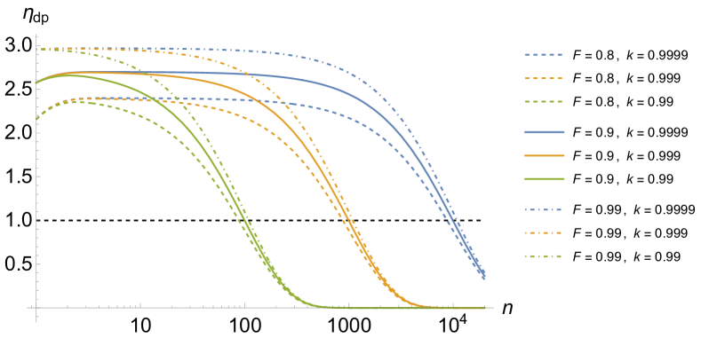
Figure 1: Visualization of $\eta_{\mathrm{dp}}$ as function of the number of local qubits $n$, for some choices of initial fidelity $F$ and local entanglement generation quality $k$. We fix $d=3$ while varying $F$ and $k$. Dashed curves correspond to $F=0.8$; solid curves correspond to $F=0.9$; dot-dashed curves correspond to $F=0.99$. Blue color represents $k=0.9999$; yellow color represents $k=0.999$; green color represents $k=0.99$.

Imperfect local entanglement generation.—We now start to include imperfections in local entanglement generation. Specifically, we consider the following phenomenological model to reflect the fidelity decrease when adding more qubits to the GHZ state: We assume that the state after local entanglement generation is an $nd$-qubit depolarized GHZ state, while the fidelity is modified according to the number of local qubits as $F(n)=k^{n-1}F$, where $F$ is the fidelity of the initial $d$-qubit GHZ state, and $k\in(0,1)$ is a parameter which describes the quality of local entanglement generation and thus the larger the better. The intuition behind this phenomenological model is the usage of noisy CNOT gates to generate GHZ states, and $k$ can be interpreted as gate fidelity. We can then express $C$ in Eqn. 2 as:

$$C_{\mathrm{dp}}(F,d,n,k)=\frac{(1-k^{n-1}F)(4^{nd}k^{n-1}F-2^{nd}-2)}{[(2^{nd}-2)k^{n-1}F+1](2^{nd}-1)}.$$ (6)

It can be shown that, as intuitively expected, $C_{\mathrm{dp}}$ decreases monotonically as initial fidelity $F$, number of local parameters $d$, and local entanglement generation quality $k$, increase for all $n\geq 1$, if $F,k>2^{-d}$. On the other hand, the dependence of $C_{\mathrm{dp}}$ on number of local quantum sensors $n$ is more complicated. We visualize $\eta_{\mathrm{dp}}=d(1-C_{\mathrm{dp}})$ with varying $n$ under different parameter choices in Fig. 1.

From the plot we can verify that the relative advantage $\eta_{\mathrm{dp}}$ is larger when $F,k$ increase. We can also see non-monotonic behavior of $\eta_{\mathrm{dp}}$ when $k$ is sufficiently high in comparison to $F$, which indicates an increase in relative advantage for small local sensor numbers. The intersection point at which $\eta_{\mathrm{dp}}=1$ determines the maximal number of local quantum sensors $n_{\mathrm{max}}$ for quantum advantage over the optimal local sensing strategy to be potentially demonstrated. We observe that $n_{\mathrm{max}}$ does not change much when varying $F$ given fixed $k$, but it changes significantly when fixing $F$ and varying $k$, which suggests that the initial fidelity $F$ has less impact on $n_{\mathrm{max}}$ than the local entanglement generation quality $k$. This can be understood by considering the fidelity threshold for the $nd$-qubit depolarized GHZ state to be advantageous over the optimal local strategy, which also scales as $1/d$ and is almost independent of $n$. Imperfect local entanglement generation will decrease the GHZ fidelity to the threshold at $n_{\mathrm{max}}$. Therefore, we expect $k^{n_{\mathrm{max}}-1}F\approx 1/d$, which gives $n_{\mathrm{max}}\approx-\ln(dF)/\ln(k)$. This also implies robustness of the quantum advantage in DQS against the imperfection of probe state generation over realitic quantum networks. See more details in Sec. III.B of the Supplemental Material [59].

Local measurement constraint.—It is possible that the optimal measurement to saturate the QCRB is entangling between the sensor nodes. In the DQS setup, entangling measurement needs additional remote entanglement as a resource to implement. Therefore, we want to use only local operations and classical communication (LOCC) [63] to extract information in DQS problems. However, in general LOCC is not guaranteed to saturate the QCRB in DQS [64]. Here we explicitly consider the local measurement constraint.

It is known that $M=\sigma_{x}^{\otimes nd}$ is the optimal observable for $nd$-qubit pure GHZ probe state under unitary z-direction phase accumulation [60], and in principle each sensor node only needs to perform measurement of the local observable $\sigma_{x}^{\otimes n}$. However, this optimal measurement under ideal conditions is genuinely useless whenever there is any noise in the GHZ state as probe. Specifically, the variance of parameter estimation will diverge when taking the limit of small local parameters. We note that this conclusion is also implied by numerical results in another recent work by Cao and Wu [65]. In Sec. IV.A of the Supplemental Material [59] we analytically demonstrate this property for the depolarized GHZ state, while it holds generally for any GHZ-diagonal state with non-unit fidelity.

Motivated by our problem formulation that the parameter to estimate is encoded through z-direction phase accumulation, we further explore the optimization over a subset of local measurements, i.e. the tensor product of single-qubit measurements along a direction on the equator of the Bloch sphere: $M(\alpha)=\left[O(\alpha)\right]^{\otimes nd}$ where $O(\alpha)=|\psi^{+}(\alpha)\rangle\langle\psi^{+}(\alpha)|-|\psi^{-}(\alpha)\rangle\langle\psi^{-}(\alpha)|$ with $|\psi^{\pm}(\alpha)\rangle=(|0\rangle\pm e^{i\alpha}|1\rangle)$ (thus $O(\alpha)=e^{i\alpha}|1\rangle\langle 0|+e^{-i\alpha}|0\rangle\langle 1|$), characterized by the azimuthal angle $\alpha$. For an $nd$-qubit depolarized GHZ state, the optimal azimuthal angle is $\alpha_{\mathrm{opt}}=\frac{2l+1}{2nd}\pi,\ l\in\mathbb{Z}$. Note that the optimal azimuthal angle depends on number of local quantum sensors $n$ and sensor node number $d$. Moreover, the estimation variance diverges quickly when $\alpha$ deviates from $\alpha_{\mathrm{opt}}$. This implies that the accuracy of local operation is extremely important, and potentially more important than the quality of the entangled states distributed by quantum networks.

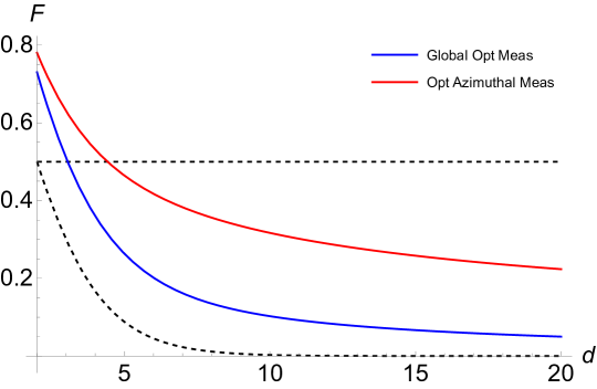
Figure 2: Visualization of fidelity thresholds. The blue solid curve denotes the fidelity threshold given by the QFI, and the threshold given by optimized local azimuthal measurement is shown as the red solid curve. The horizontal and curved black dashed lines again represent the fidelity thresholds for $d$-qubit depolarized GHZ state to be GME and non-fully separable, respectively.

The fidelity threshold for an $nd$-qubit depolarized GHZ state to be advantageous over the optimal local strategy when using the optimized azimuthal measurement is:

$$F_{\mathrm{th},M(\alpha_{\mathrm{opt}})}(n)=\frac{2^{nd}+\sqrt{d}-1}{2^{nd}\sqrt{d}}.$$ (7)

The case of $n=1$ for Eq. 7 corresponds to noiseless local entanglement generation, similar to Eq. 5. We thus visualize and compare both fidelity thresholds in Fig. 2. The fidelity threshold in Eq. 7 is always higher than that given by Eq. 5, suggesting that the optimized local azimuthal measurement does not saturate the QCRB. On the other hand, although for small problem sizes $d<5$ the initial GHZ state needs to be GME to demonstrate quantum advantage if we use the optimized azimuthal measurement, when the problem size grows the requirement of initial fidelity drops, and in general the initial $d$-qubit GHZ state does not have to be GME. More details on the azimuthal measurement optimization can be found in Sec. IV.B of the Supplemental Material [59].

Table 1: Simulation results for the three scenarios.

	$p$	$\eta$	$\tilde{\eta}$	$F$
Scenario 1	$\approx 0.02$	$\approx 0.95<1$	$\approx 0.02<1$	0.591
Scenario 2	$\approx 0.72$	$\approx 1.57>1$	$\approx 1.13>1$	0.732
Scenario 3	$\approx 0.81$	$\approx 2.19>1$	$\approx 1.77>1$	0.854

Quantum network simulation.—Following the above analytics, we simulate GHZ state distribution given realistic first-generation quantum repeater [66, 67, 68] protocol stacks with an open-source, customizable quantum network simulator, SeQUeNCe [69]. We consider a simple 3-node network with linear topology, where a center node directly connects the other two end nodes through optical fibers, with a Bell state measurement station in the middle of each fiber link. First, bipartite entanglement links are established between the center node and the other nodes. Then LOCC, such as gate teleportation [70, 71, 72] and graph state fusion [73, 74], are performed to generate a GHZ state across all network nodes.

In our simulations we consider three scenarios, and thus three sets of system parameter values: $\{0.01\mathrm{s},0.1\mathrm{s},1\mathrm{s}\}$ for memory coherence times, $\{0.05,0.1,0.5\}$ for memory efficiency, and $\{0.8,0.85,0.9\}$ for raw entanglement fidelity. The first simulation scenario uses the first value in each of the above sets, and so on. Meanwhile, we fix other system parameters, especially: a 1s time interval allowed for entanglement distribution, a 10km distance between the center node and end nodes, 10 memories per end node and 20 memories on the center node so that entanglement purification [75, 76] is possible. We emphasize that the parameter values are not chosen from a specific reported experiment, but are selected according to the general vision of the state of the art and the potential future development of various candidate platforms for quantum networking, including solid state systems [28, 30, 77], atomic systems [29, 78], and superconducting systems [79]. Details of our quantum network simulation can be found in Sec. VII of the Supplemental Material [59].

We characterize the performance of probe state distribution by three figures of merit, namely the success probability of distributing the 3-qubit GHZ state, $p$, the relative advantage, $\eta$, and the normalized relative advantage, $\tilde{\eta}=p\cdot\eta$, which takes into account failure in entanglement distribution (See Sec. V of the Supplemental Material [59]). For each scenario we repeat the simulation 1000 times, and $\eta$ is calculated based on the average of density matrices of successfully distributed GHZ states under ensemble interpretation. The results are collected in Table 1, from which it is clear that the most modest parameter choice does not permit quantum advantage, while when hardware performance improves quantum advantage becomes possible without changing the realistic quantum network protocol stack. We also note the average fidelity $F$ of the successfully generated states for each scenario; as expected, the fidelity increases as the network parameters improve.

Conclusion and discussion.—In summary, we perform extensive analytical studies on the impact of imperfect GHZ state distributed by noisy quantum networks on DQS. Our results offer new insights into realistic DQS, and reveal the relation between entanglement and DQS quantum advantage. We also simulate the GHZ state distribution process over a 3-node quantum network, demonstrating the possibility of DQS quantum advantage with realistic quantum network stacks. The new features we develop in SeQUeNCe to reflect imperfections in entanglement distribution are completely open-source [80], and can thus serve as valuable resources for future quantum network research. We leave more detailed quantum network simulation as a followup work.

We have primarily focused on probe state preparation errors, while the parameter encoding dynamics can also be noisy due to sensor decoherence. It could be interesting to evaluate the impact of sensor decoherence after state preparation [81], where the time dependence of estimation accuracy gain [82, 83, 84] becomes important. We note that quantum error correction [85, 86, 87, 88] offers a good opportunity in fighting against noise in sensing process. Meanwhile, protocols such as continuous entanglement distribution [89, 90, 91] might be necessary to reduce latency of probe state preparation over quantum networks. In addition, optimization of Bell-state-based graph state distribution [92, 93, 94, 95, 96, 97, 98, 99, 100] is important for larger scale DQS. Notably, privacy and security [101, 102, 103] is a potentially important aspect of realistic quantum sensor network as well. Finally, although we mainly assume finite-dimensional matter-based quantum sensors, photonic systems [104, 105, 106, 107, 108, 109] are also playing an important role in DQS.

Acknowledgments.—A.Z. would like to thank Tian-Xing Zheng and Boxuan Zhou for helpful discussions. This material is based upon work supported by the U.S. Department of Energy Office of Science National Quantum Information Science Research Centers. Work performed at the Center for Nanoscale Materials, a U.S. Department of Energy Office of Science User Facility, was supported by the U.S. DOE, Office of Basic Energy Sciences, under Contract No. DE-AC02-06CH11357. A.Z. and T.Z. are also supported by the NSF Quantum Leap Challenge Institute for Hybrid Quantum Architectures and Networks (NSF Grant No. 2016136), and the Marshall and Arlene Bennett Family Research Program.

The submitted manuscript has been created by UChicago Argonne, LLC, Operator of Argonne National Laboratory (“Argonne”). Argonne, a U.S. Department of Energy Office of Science laboratory, is operated under Contract No. DE-AC02-06CH11357. The U.S. Government retains for itself, and others acting on its behalf, a paid-up nonexclusive, irrevocable worldwide license in said article to reproduce, prepare derivative works, distribute copies to the public, and perform publicly and display publicly, by or on behalf of the Government. The Department of Energy will provide public access to these results of federally sponsored research in accordance with the DOE Public Access Plan. http://energy.gov/downloads/doe-public-access-plan.

Supplemental Material

I Multiparameter estimation

In this section we provide the background information for distributed quantum sensing problem, including multiparameter estimation, classical and quantum Fisher information matrix, classical and quantum Cramér-Rao bound, and estimating linear function of local parameters.

I.1 (Quantum) Cramér-Rao bound

In a general multiparameter estimation problem, there are $d$ parameters $x=(x_{1},\dots,x_{d})^{T}\in\mathbb{R}^{d}$ to be estimated. To perform the estimation, a collection of statistical data (sample) $s=(s_{1},\dots,s_{\mu})^{T}\in\mathbb{R}^{\mu}$ are accumulated from $\mu$ times of measurement. In the so-called probabilistic approach of estimation, it is assumed that the measured data are random numbers subject to a probability distribution $p(s|x)$ which is dependent on the parameters. An estimator $\hat{x}$ is a rule for calculating the estimate value of parameters based on the measured data. For an estimator, its quality can be characterized by the covariance matrix:

$$\left(\mathrm{Cov}(\hat{x})\right)_{ij}=\mathbb{E}\left[(\hat{x}_{i}-\mathbb{E}[\hat{x}_{i}])(\hat{x}_{j}-\mathbb{E}[\hat{x}_{j}])\right],$$ (8)

where $\mathbb{E}[\cdot]$ denotes the estimation value of a certain random variable. It is commonly assumed that the estimator is locally unbiased, i.e. $\mathbb{E}[\hat{x}_{i}]=x_{i}$. It is well known that the covariance matrix of any locally unbiased estimator obeys the Cramér-Rao bound (CRB):

$$\mathrm{Cov}(\hat{x})\succeq\frac{\mathcal{I}^{-1}}{\mu},$$ (9)

where for matrices $A\succeq B$ means that the matrix difference $(A-B)$ is positive semidefinite, $N$ is the number of data points in the sample, and $\mathcal{I}$ is the classical Fisher information matrix (CFIM):

$$\mathcal{I}_{ij}=\mathbb{E}\left[\frac{\partial\ln p(s|x)}{\partial x_{i}}\frac{\partial\ln p(s|x)}{\partial x_{j}}\right].$$ (10)

Note that the CRB holds when the CFIM is invertible, i.e. positive definite given its symmetric nature.

When performing multiparameter estimation using quantum mechanical systems, the parameters are usually encoded in the quantum state $\rho_{x}$. The process of obtaining data points through measurement can then be described by POVMs $\{\Pi_{s}\}$ which satisfy normalization $\sum_{s}(\int_{s})\Pi_{s}=I$. That is, now the probability distribution of sample data points is $p(s|x)=\mathrm{tr}(\rho_{x}\Pi_{s})$, from which the CFIM can be calculated.

The quantum Fisher information matrix (QFIM) $\mathcal{F}$ is defined through symmetric logarithmic derivatives (SLD) with respect to different single parameters:

$$\mathcal{F}_{ij}=\mathrm{Tr}\left(\rho\frac{L_{i}L_{j}+L_{j}L_{i}}{2}\right),$$ (11)

where $L_{i}$ is the SLD for parameter $x_{i}$, s.t.

$$\frac{\partial}{\partial x_{i}}\rho\coloneqq\partial_{i}\rho=\frac{1}{2}\{\rho,L_{i}\}.$$ (12)

The QFIM satisfies $\mathcal{F}\succeq\mathcal{I}_{\Pi}$, for arbitrary POVM $\{\Pi\}$ applied on $\rho_{x}$. Therefore, we can use the QFIM to bound the covariance matrix of any locally unbiased estimator $\hat{x}$:

$$\mathrm{Cov}(\hat{x})\succeq\frac{\mathcal{I}^{-1}}{\mu}\succeq\frac{\mathcal{F}^{-1}}{\mu},$$ (13)

which is known as the quantum Cramér-Rao bound (QCRB).

I.2 Estimating functions of parameters

Besides “naturally” encoded parameters, we might want to estimate functions of them. That is, we can consider $d$ new parameters $\theta=(f_{1}(x),\dots,f_{d}(x))^{T}\in\mathbb{R}^{d}$. It turns out that the QFIM of the derived parameters $\theta$ can be expressed in terms of the QFIM of the original parameters $x$ as [55]:

$$\mathcal{F}(\theta)=J^{T}\mathcal{F}(x)J,$$ (14)

where $J$ is the Jacobian matrix whose matrix elements are $J_{ij}=\partial x_{i}/\partial\theta_{j}$. Then the QCRB for the estimator $\hat{\theta}$ of the derived parameters becomes:

$$\mathrm{Cov}(\hat{\theta})\succeq\frac{\mathcal{F}^{-1}(\theta)}{\mu}.$$ (15)

In some cases such as this work, we may focus on linear functions of parameters:

$$\theta=Mx,$$ (16)

where without loss of generality we require that all rows of $M$ are linearly independent. Then the Jacobian is simply $J=M^{-1}$. Now consider the case where we are only interested in one specific parameter as a linear function of $d$ parameters, $\theta_{1}=v_{1}^{T}x$. We may construct $(d-1)$ additional vectors $v_{i}$, $i=2,\dots,d$ that are mutually linearly independent, and also linearly independent of $v_{1}$. Then we construct $M=(v_{1},\dots,v_{d})^{T}$ which determines $n$ derived parameters, with $\theta_{1}=(Mx)_{1}$. The variance of estimating the single derived parameter $\theta_{1}$ is then bounded from the QCRB [55]:

$$\mathrm{Var}(\hat{\theta}_{1})\geq\frac{\left(\mathcal{F}^{-1}(\theta)\right)_{11}}{\mu}=\frac{\left(J^{-1}\mathcal{F}^{-1}(x)(J^{T})^{-1}\right)_{11}}{\mu},$$ (17)

at fixed values of other derived parameters $\theta_{2},\dots,\theta_{n}$, which is valid in that the additional parameters are constructed to be linearly independent of the single parameter of our interest.

II Quantum Fisher information matrix under unitary encoding

Suppose the encoded state has spectral decomposition $\rho=\sum_{a}\lambda_{a}|\psi_{a}\rangle\langle\psi_{a}|$ with all $\lambda_{a}$ being non-zero. Then the QFIM can be expressed as [58]

$$\mathcal{F}_{ij}= \sum_{a}\frac{(\partial_{i}\lambda_{a})(\partial_{j}\lambda_{a})}{\lambda_{a}}+\sum_{a}4\lambda_{a}\mathrm{Re}(\langle\partial_{i}\psi_{a}|\partial_{j}\psi_{a}\rangle)-\sum_{a,b}\frac{8\lambda_{a}\lambda_{b}}{\lambda_{a}+\lambda_{b}}\mathrm{Re}(\langle\partial_{i}\psi_{a}|\psi_{b}\rangle\langle\psi_{b}|\partial_{j}\psi_{a}\rangle).$$ (18)

We note that there are different equivalent ways of calculating QFIM, as documented in some other extensive reviews, for instance [55, 56, 57].

Then we consider that the parameter dependence of $\rho$ comes from unitary encoding $U(x)$ of an $x$-independent initial state $\rho_{0}=\sum_{a}\lambda_{a0}|\psi_{a0}\rangle\langle\psi_{a0}|$, i.e. $\rho=U(x)\rho_{0}U(x)^{\dagger}$. Now the QFIM can be re-expressed in the convention of [58] as:

$$\mathcal{F}_{ij}=\sum_{a}4\lambda_{a0}\mathrm{cov}_{|\psi_{a0}\rangle}(G_{i},G_{j})-\sum_{a\neq b}\frac{8\lambda_{a0}\lambda_{b0}}{\lambda_{a0}+\lambda_{b0}}\mathrm{Re}(\langle\psi_{a0}|G_{i}|\psi_{b0}\rangle\langle\psi_{b0}|G_{j}|\psi_{a0}\rangle),$$ (19)

where $\mathrm{cov}_{|\psi\rangle}(A,B)$ denotes the covariance of observables $A$ and $B$ under a pure state $|\psi\rangle$:

$$\mathrm{cov}_{|\psi\rangle}(A,B)=\frac{1}{2}\langle\psi|\{A,B\}|\psi\rangle-\langle\psi|A|\psi\rangle\langle\psi|B|\psi\rangle,$$ (20)

and $G_{i}$ is the generator of parameter $x_{i}$:

$$G_{i}=i(\partial_{i}U^{\dagger})U=-iU^{\dagger}(\partial_{i}U).$$ (21)

II.1 GHZ-diagonal state with collective spin phase accumulation

Consider that the parameter encoding is through $U(x)=\exp\left[-i\left(\sum_{i=0}^{d-1}x_{i}H_{i}\right)\right]$, where $d$ denotes the total number of sensor nodes in the network, $H_{i}=\frac{1}{2}\sum_{k=0}^{n-1}\sigma^{(i,k)}_{z}$ is the local collective spin of $n$ qubit sensors on node $i$, and the parameters $x_{i}$ physically correspond to accumulated phases through Hamiltonian evolution. It can thus be easily verified that the generators according to the above definition are $G_{i}=-H_{i}$, where the negative sign does not matter as generators appear in pairs in Eqn. 19. Then for $\rho_{0}$ which is a GHZ-diagonal state, we have that:

$$\mathrm{cov}_{|\psi_{m0}\rangle}(G_{i},G_{j})= \mathrm{cov}_{|\psi_{m0}\rangle}(H_{i},H_{j})=\frac{1}{2}\langle\psi_{m0}|\{H_{i},H_{j}\}|\psi_{m0}\rangle,\ \forall m,$$ (22)

because weight-1 Pauli strings do not stabilize the standard GHZ states. Meanwhile, we have that:

$$\langle\psi|\sigma_{z}^{(a)}\sigma_{z}^{(b)}|\psi\rangle=1,\ \forall a,b,$$ (23)

where $a,b$ are indices for the qubits in $|\psi\rangle$ which is a GHZ-basis state. This is because weight-2 Pauli strings with only Pauli Z operators stabilize the standard GHZ states. Therefore, for any GHZ-diagonal $\rho_{0}$, the first single-index sum in Eqn. 19 is always a constant:

$$\sum_{a}4\lambda_{a0}\mathrm{cov}_{|\psi_{a0}\rangle}(G_{i},G_{j})= \sum_{a}4\lambda_{a0}\mathrm{cov}_{|\psi_{a0}\rangle}\left(\frac{1}{2}\sum_{k=0}^{n-1}\sigma^{(i,k)}_{z},\frac{1}{2}\sum_{l=0}^{n-1}\sigma^{(j,l)}_{z}\right)$$

$$= \sum_{a}\lambda_{a0}\sum_{k=0}^{n-1}\sum_{l=0}^{n-1}\mathrm{cov}_{|\psi_{a0}\rangle}\left(\sigma^{(i,k)}_{z},\sigma^{(j,l)}_{z}\right)=n^{2},\ \forall i,j,$$ (24)

which reveals the Heisenberg scaling with number of local qubit sensors. Then the derivation of the QFIM reduces to the second term in Eqn. 19.

There are $2^{nd}$ orthonormal $nd$-qubit GHZ states across $d$ sensor nodes where each node holds $n$ qubits, which can be labeled by the binary string from 0 through $2^{nd-1}-1$: These states are superpositions of two computational basis states which correspond to binary strings of $b\in\{0,1,\dots,2^{nd-1}-1\}$ and $2^{nd}-b-1$, respectively. The additional $2^{nd-1}$ states come from adding an additional $\pi$ relative phase between the two computational basis states. Notice that for any GHZ state $|\psi\rangle$, the application of a single Pauli Z operator on it will lead to a $\pi$ change in the relative phase between the two computational basis states in superposition. Therefore, $\langle\psi_{a0}|G_{i}|\psi_{b0}\rangle$ is either zero due to orthogonality between $|\psi_{a0}\rangle$ and $G_{i}|\psi_{b0}\rangle$, or one, and it takes unit value only when $|\psi_{a0}\rangle$ and $|\psi_{b0}\rangle$ correspond to the same length-$nd$ binary string and have relative phases which differ by $\pi$.

For a general $nd$-qubit GHZ-diagonal state $\rho_{0}=\sum_{a}\lambda_{a0}|\psi_{a0}\rangle\langle\psi_{a0}|$ where each node has $n$ qubits, we use $\mathcal{S}$ to denote the set of index pairs $(a,b)$ such that $|\psi_{a0}\rangle$ and $|\psi_{b0}\rangle$ are GHZ states as superposition of the same pair of computational basis states but with opposite relative phase. Note that for such pairs, $(a,b)$ and $(b,a)$ are both included in set $\mathcal{S}$. Then we have:

$$\sum_{a\neq b}\frac{8\lambda_{a0}\lambda_{b0}}{\lambda_{a0}+\lambda_{b0}}\mathrm{Re}(\langle\psi_{a0}|G_{i}|\psi_{b0}\rangle\langle\psi_{b0}|G_{j}|\psi_{a0}\rangle)=n^{2}\sum_{(a,b)\in\mathcal{S}}\frac{2\lambda_{a0}\lambda_{b0}}{\lambda_{a0}+\lambda_{b0}}=Cn^{2},\ \forall i,j,$$ (25)

which again does not depend on $i,j$, and will only modify the Heisenberg scaling factor, while we comment that in practice $C$ can be dependent on $n$. We may consider a special case as example: We assume noiseless local entanglement generation when extending any $d$-qubit GHZ state into $nd$-qubit GHZ state involving $n-1$ additional qubits per node, and the result is simply duplicating each binary digit of the binary strings that represent the computational basis. For instance, $(|000\rangle+|111\rangle)/\sqrt{2}$ will be extended to $(|\tilde{0}_{n}\tilde{0}_{n}\tilde{0}_{n}\rangle+|\tilde{1}_{n}\tilde{1}_{n}\tilde{1}_{n}\rangle)/\sqrt{2}$, where $\tilde{i}_{n}=\underbrace{i\dots i}_{\text{$n$ digits}}$. In this example $C$ is indeed a constant that only depends on the initial $d$-qubit GHZ state.

We also comment that the form of the series in Eqn. 25 implies that only Pauli Z errors affect the QFIM, which is a result of our assumed encoding channel, i.e. a z-axis coupling. Additionally, we note that the maximum value of $C$ is 1 for GHZ-diagonal states, and it is achieved if and only if every pair of states in set $\mathcal{S}$ have identical eigenvalues. This can be seen as follows:

$$C= \sum_{(a,b)\in\mathcal{S}}\frac{2\lambda_{a0}\lambda_{b0}}{\lambda_{a0}+\lambda_{b0}}=\frac{1}{2}\sum_{(a,b)\in\mathcal{S}}\frac{(\lambda_{a0}+\lambda_{b0})^{2}-(\lambda_{a0}-\lambda_{b0})^{2}}{\lambda_{a0}+\lambda_{b0}}$$

$$= \frac{1}{2}\sum_{(a,b)\in\mathcal{S}}(\lambda_{a0}+\lambda_{b0})-\frac{1}{2}\sum_{(a,b)\in\mathcal{S}}\frac{(\lambda_{a0}-\lambda_{b0})^{2}}{\lambda_{a0}+\lambda_{b0}}$$

$$= 1-\frac{1}{2}\sum_{(a,b)\in\mathcal{S}}\frac{(\lambda_{a0}-\lambda_{b0})^{2}}{\lambda_{a0}+\lambda_{b0}},$$ (26)

where the subtracted term is non-negative, and it becomes zero if and only if $\lambda_{a0}=\lambda_{b0}$, $\forall(a,b)\in\mathcal{S}$.

Combining the above results, we can explicitly write the QFIM with respect to local parameters $x=(x_{1},\dots,x_{d})^{T}$ as:

$$\mathcal{F}(x)=(1-C)n^{2}\begin{pmatrix}1&1&\dots&1\\ 1&1&\dots&1\\ \vdots&\vdots&\ddots&\vdots\\ 1&1&\dots&1\\ \end{pmatrix}.$$ (27)

According to the parameter estimation problem of our interest, we have that $v_{1}\propto(1,\dots,1)^{T}\in\mathbb{R}^{d}$. For concreteness, we may choose $v_{1}=(1,\dots,1)/\sqrt{d}$, which is a normalized vector under 2-norm. As now we only focus on estimating one parameter $v_{1}^{T}x$, we can construct an orthonormal matrix $M=(v_{1},\dots,v_{d})^{T}$ such that $v_{i}^{T}v_{j}=\delta_{ij}$. Then according to Eqn. 14 we have the QFIM with respect to new parameters $\theta=(v_{1}^{T}x,\dots,v_{d}^{T}x)$:

$$\mathcal{F}(\theta)= \sqrt{d}(1-C)n^{2}\begin{pmatrix}v_{1}^{T}\\ v_{2}^{T}\\ \vdots\\ v_{d}^{T}\\ \end{pmatrix}\begin{pmatrix}v_{1}&v_{1}&\dots&v_{1}\end{pmatrix}\begin{pmatrix}v_{1}&v_{2}&\dots&v_{d}\end{pmatrix}$$

$$= \sqrt{d}(1-C)n^{2}\begin{pmatrix}1&1&\dots&1\\ 0&0&\dots&0\\ \vdots&\vdots&\ddots&\vdots\\ 0&0&\dots&0\\ \end{pmatrix}\begin{pmatrix}v_{1}&v_{2}&\dots&v_{d}\end{pmatrix}$$

$$= d(1-C)n^{2}\begin{pmatrix}v_{1}^{T}\\ 0\\ \vdots\\ 0\\ \end{pmatrix}\begin{pmatrix}v_{1}&v_{2}&\dots&v_{d}\end{pmatrix}=d(1-C)n^{2}\begin{pmatrix}1&0&\dots&0\\ 0&0&\dots&0\\ \vdots&\vdots&\ddots&\vdots\\ 0&0&\dots&0\\ \end{pmatrix}.$$ (28)

II.2 Lower bound of QFI for a fixed fidelity

Given the analytical formula of calculating the $C$ term in QFI expression, we could evaluate the lower bound of QFI for all possible GHZ-diagonal states with a fixed fidelity. We could prove the following result.

Proposition II.1.

For $d$-qubit GHZ-diagonal states with a fixed fidelity $F\in(0,1)$, the lowest QFI for estimating the average of $d$ local parameters is $d(2F-1)^{2}$.

Proof.

We label the the eigenvalues of the density matrix in the following way. Consider that GHZ states can be expressed as a superposition of two computational basis states, which correspond to two binary strings, and one of the binary string corresponds to a smaller integer $n\in\{0,1,\dots,2^{d-1}-1\}$ while the other corresponds to a larger integer $m=2^{d}-n-1$. For a GHZ state expressed as a superposition of computational basis state corresponding to $n$ and $m$ with $n<m$, we let its index be $2n$ if the relative phase between two computational basis states is $0$, and $2n+1$ otherwise. For instance, the standard GHZ state $|\mathrm{GHZ}_{d}\rangle$ has index 0, and $Z|\mathrm{GHZ}_{d}\rangle$ has index 1. Then we have that the eigenvalue corresponding to $|\mathrm{GHZ}_{d}\rangle$ is $\lambda_{00}=F$. For the rest $2^{d}-1$ eigenvalues with $i\in\{1,2,\dots,2^{d}-1\}$, we can express them as $\lambda_{i0}=(1-F)p_{i}$, s.t. $p_{i}\in[0,1]$ and $\sum_{i=1}^{2^{d}-1}p_{i}=1$.

Then the objective is transformed to finding the combination of $(p_{1},\dots,p_{2^{d}-1})$ which gives the highest $C$ under the above constraints. The constraints clearly define a closed and compact region $\mathcal{R}$. Then according to the extreme value theorem, we are sure that there exists a maximum value and a minimum value for any continuous function of $(p_{1},\dots,p_{2^{d}-1})$ on $\mathcal{R}$, and the extreme values must be taken either on the boundary of $\mathcal{R}$, or at critical points inside $\mathcal{R}$.

Now $C$ can be re-written as:

$$C=\frac{4F(1-F)p_{1}}{F+(1-F)p_{1}}+\sum_{i=1}^{2^{d-1}-1}\frac{4(1-F)p_{2i}p_{2i+1}}{p_{2i}+p_{2i+1}},$$ (29)

which is obviously continuous on $\mathcal{R}$. We first take the partial derivatives with respect to $p_{i}$:

$$\frac{\partial}{\partial p_{1}}C=\frac{4(1-F)F^{2}}{\left[F+(1-F)p_{1}\right]^{2}}>0,$$ (30)

$$\frac{\partial}{\partial p_{i}}C=\frac{4(1-F)p_{i+(-1)^{i\,\mathrm{mod}\,2}}^{2}}{\left(p_{i}+p_{i+(-1)^{i\,\mathrm{mod}\,2}}\right)^{2}}\geq 0,~{}i>1,$$ (31)

which means that there is no critical point inside $\mathcal{R}$, so the maximum value can only be on the boundary of $\mathcal{R}$.

It is clear that the boundary of $\mathcal{R}$ can be divided into $2^{d}-1$ parts $\{B_{i}\}$, each determined by $p_{i}=0$ for a specific $i\in\{1,2,\dots,2^{d}-1\}$. Under the equality constraint $\sum_{i=1}^{2^{d}-1}p_{i}=1$, the above partial derivatives suggest that there is still no critical point inside any $B_{i}$. This means that the extreme values on the boundary should be on the boundary of $B_{i}$, i.e, $\{B_{ij}\}$, where the subscript means the $j$-th part of the boundary of $B_{i}$. The conclusion of no inside critical point holds until we have reduced the boundary into zero-dimension points, characterized by $p_{i}=1$.

Finally, we can compare the $C$ values for all the $2^{d}-1$ choices of $(p_{1},\dots,p_{2^{d}-1})$. It is obvious that if $p_{i}=1$ and $i>1$, $C=0$, and if $p_{1}=1$, $C=4F(1-F)>0$. Therefore, the maximal value of $C$ on $\mathcal{R}$ is $4F(1-F)$ corresponding to $\rho=F|\mathrm{GHZ}_{d}\rangle\langle\mathrm{GHZ}_{d}|+(1-F)Z|\mathrm{GHZ}_{d}\rangle\langle\mathrm{GHZ}_{d}|Z$, which gives the lowest QFI $\mathcal{F}=d(1-C)=d(2F-1)^{2}$. ∎

The physical interpretation of this result is clear. The worst-case scenario can be interpreted as that all probe state preparation error is indistinguishable from the signal of the parameter to estimate, because of our assumption that the parameter is encoded through z-component phase accumulation. On the other hand, the QFI for noisy GHZ state can be equal to that for noiseless GHZ state, and this can be interpreted as that when probe state error can be distinguished from the signal, it is still possible to extract the information encoded in the “noisy” components of the probe state.

III Analytics for depolarized GHZ state

III.1 Noiseless local entanglement generation

We consider $d$-qubit GHZ states under collective depolarizing channel which is characterized by a single parameter, the fidelity $F$: $\rho_{d,0}(F)=\frac{2^{d}F-1}{2^{d}-1}|\mathrm{GHZ}_{d}\rangle\langle\mathrm{GHZ}_{d}|+\frac{1-F}{2^{d}-1}I$. For this specific family of states, we can obtain the closed form expression of the constant $C$ in Eqn. 25:

$$C_{\mathrm{dp}}= 2\left[\frac{2F\frac{1-F}{2^{d}-1}}{F+\frac{1-F}{2^{d}-1}}+(2^{d-1}-1)\frac{2\left(\frac{1-F}{2^{d}-1}\right)^{2}}{2\frac{1-F}{2^{d}-1}}\right]=\frac{(1-F)(4^{d}F-2^{d}-2)}{[(2^{d}-2)F+1](2^{d}-1)}.$$ (32)

It is obvious that both the numerator and the denominator are positive, and then we take the difference between the numerator and the denominator:

$$(1-F)(4^{d}F-2^{d}-2)-[(2^{d}-2)F+1](2^{d}-1)=-(2^{d}F-1)^{2}<0,$$ (33)

which means that $0\leq C_{\mathrm{dp}}<1$. Then we examine $\eta_{\mathrm{dp}}=d(1-C_{\mathrm{dp}})$:

$$\frac{\partial}{\partial F}\eta_{\mathrm{dp}}=\frac{d\left[2-3\times 2^{d}+2^{2d+1}F+(2^{d}-2)4^{d}F^{2}\right]}{(2^{d}-1)\left[(2^{d}-2)F+1\right]^{2}},$$ (34)

whose sign is only determined by the numerator. It is easy to find that the above partial derivative equals zero at $F=2^{-d}$ and $F=(2-3\times 2^{d})/(4^{d}-2^{d+1})<0$. That is, the partial derivative is negative for $F\in[0,2^{-d})$ and positive for $F\in(2^{-d},1]$, which means that for fixed $d$ the minimal value of $\eta_{\mathrm{dp}}$ is taken at $F=2^{-d}$. This fidelity corresponds to a $d$-qubit maximally mixed state, and the minimal value is:

$$\left.\eta_{\mathrm{dp}}\right|_{F=2^{-d}}=0.$$ (35)

This is because unitary encoding does not vary the maximally mixed state and then any following measurement will not be able to extract information of the encoded parameters.

We solve the equation $C_{\mathrm{dp}}=(d-1)/d$, whose only positive solution is the fidelity threshold for depolarized GHZ states to demonstrate advantage in estimating the average of local parameters over the optimal local strategy:

$$F_{\mathrm{th,dp}}=2^{-d}+\frac{(2^{d}-1)\left(2^{d}-2+\sqrt{(2^{d}-2)^{2}+2^{d+3}d}\right)}{2^{2d+1}d}.$$ (36)

It can be shown that:

Proposition III.1.

$F_{\mathrm{th,dp}}>3/(2^{d}+2)$ for $d\geq 2$.

Proof.

First notice that $3/(2^{d}+2)<3/2^{d}$. Then we take the difference $F_{\mathrm{th,dp}}-3/2^{d}$ as:

$$F_{\mathrm{th,dp}}-\frac{3}{2^{d}}=\frac{(2^{d}-1)\left(2^{d}-2+\sqrt{(2^{d}-2)^{2}+2^{d+3}d}\right)-2^{d+2}d}{2^{2d+1}d},$$ (37)

whose positivity is only determined by the numerator. Then notice that $2^{d}-1\geq 2^{d}-2\geq 2^{d-1}$ for $d\geq 2$. Thus we can relax the first product in the numerator:

$$(2^{d}-1)\left(2^{d}-2+\sqrt{(2^{d}-2)^{2}+2^{d+3}d}\right)\geq 2^{d-1}(2^{d-1}+2^{d-1})=2^{2d-1}.$$ (38)

It is then easy to show that $2^{d-1}>4d$ for $d\geq 6$. Then with straightforward calculation, we can also verify that $F_{\mathrm{th,dp}}>3/(2^{d}+2)$ for $d=2,3,4,5$. ∎

III.1.1 Comment on rank-2 dephased GHZ state

We can also consider the worst-case scenario, i.e. the $d$-qubit rank-2 dephased GHZ state $\rho=F|\mathrm{GHZ}_{d}\rangle\langle\mathrm{GHZ}_{d}|+(1-F)Z|\mathrm{GHZ}_{d}\rangle\langle\mathrm{GHZ}_{d}|Z$. The fidelity threshold for this type of noisy GHZ state to be advantageous over the optimal sensing strategy is:

$$F_{\mathrm{th},r=2}=\frac{1+\sqrt{d}}{2\sqrt{d}}>\frac{1}{2}.$$ (39)

In fact, it can be easily shown using GME criterion in [62] that any rank-2 GHZ-diagonal state $\rho=F|\mathrm{GHZ}_{d}\rangle\langle\mathrm{GHZ}_{d}|+(1-F)P|\mathrm{GHZ}_{d}\rangle\langle\mathrm{GHZ}_{d}|P$, where $P$ is a $d$-qubit Pauli string that does not stabilize $|\mathrm{GHZ}_{d}\rangle$, is GME regardless of fidelity $F$. Therefore, although the rank-2 dephased GHZ state is always GME, it is not very metrologically useful for our task. However, in reality the prepared probe state is very unlikely to be rank-2.

III.2 Imperfect local entanglement generation

We first consider $nd$-qubit depolarized GHZ state with fidelity $F$, and the coefficient $C$ before $n^{2}$ for the second term in QFI derivation is:

$$C_{\mathrm{dp}}(F,d,n)=2\left[\frac{2F\frac{1-F}{2^{nd}-1}}{F+\frac{1-F}{2^{nd}-1}}+(2^{nd-1}-1)\frac{2\left(\frac{1-F}{2^{nd}-1}\right)^{2}}{2\frac{1-F}{2^{nd}-1}}\right]=\frac{(1-F)(4^{nd}F-2^{nd}-2)}{[(2^{nd}-2)F+1](2^{nd}-1)}.$$ (40)

Similar to perfect local entanglement generation case, we can derive the fidelity threshold for collectively depolarized $nd$-qubit GHZ state to demonstrate advantage in parameter average estimation as:

$$F_{\mathrm{th,dp}}(F,d,n)=2^{-nd}+\frac{(2^{nd}-1)\left(2^{nd}-2+\sqrt{(2^{nd}-2)^{2}+2^{nd+3}d}\right)}{2^{2nd+1}d}.$$ (41)

The threshold also quickly converges to $1/d$. Then we can express $C_{\mathrm{dp}}$ by substituting $F$ with $F(n)=k^{n-1}F$ in Eqn. 40:

$$C_{\mathrm{dp}}(F,d,n,k)=\frac{(1-k^{n-1}F)(4^{nd}k^{n-1}F-2^{nd}-2)}{[(2^{nd}-2)k^{n-1}F+1](2^{nd}-1)}.$$ (42)

We could easily prove some intuitive properties.

Proposition III.2.

Given the above model of imperfect local entanglement generation, $C_{\mathrm{dp}}$ decreases monotonically as initial fidelity $F$, number of local parameters $d$, and local entanglement generation quality $k$, increase for all $n\geq 1$, if $F,k>2^{-d}$.

Proof.

For instance, we could take its partial derivatives with respect to $F,d,k$:

$$\frac{\partial}{\partial F}C_{\mathrm{dp}}=\frac{k^{n}\left[1-(2^{d}k)^{n}\frac{F}{k}\right]\left[(3\times 2^{nd}-2)k+2^{nd}(2^{nd}-2)k^{n}F\right]}{(2^{nd}-1)\left[(2^{nd}-2)k^{n}F+k\right]^{2}},$$ (43)

$$\frac{\partial}{\partial d}C_{\mathrm{dp}}=\ln 2\frac{2^{nd}(k-k^{n}F)\left[1-(2^{d}k)^{n}\frac{F}{k}\right]\left[(3\times 2^{nd}-4)k^{n}F+k\right]n}{(2^{nd}-1)^{2}\left[(2^{nd}-2)k^{n}F+k\right]^{2}},$$ (44)

$$\frac{\partial}{\partial k}C_{\mathrm{dp}}=\frac{k^{n-1}F\left[1-(2^{d}k)^{n}\frac{F}{k}\right]\left[(3\times 2^{nd}-2)k+2^{nd}(2^{nd}-2)k^{n}F\right](n-1)}{(2^{nd}-1)\left[(2^{nd}-2)k^{n}F+k\right]^{2}}.$$ (45)

Notice that all the above partial derivatives have positive denominators for $n\geq 1$, $F\in(0,1]$, $k\in(0,1)$ and $d\geq 2$. The numerators all contain one term $\left[1-(2^{d}k)^{n}\frac{F}{k}\right]$ while the remaining terms are also positive under the parameter regime of our interest. Therefore, the positivity of the partial derivatives is only determined by the positivity of $\left[1-(2^{d}k)^{n}\frac{F}{k}\right]$. It can be easily determined that as long as $F,k>2^{-d}$ this term is negative for all $n\geq 1$. ∎

We consider the asymptotic limit of the QFI when the local entanglement generation is imperfect, i.e. $k<1$. Explicitly, we consider $\lim_{n\rightarrow\infty}d[1-C_{\mathrm{dp}}(F,d,n,k)]n^{2}$:

$$0\leq d[1-C_{\mathrm{dp}}(F,d,n,k)]n^{2}= \frac{d\left(k-2^{nd}k^{n}F\right)}{(2^{nd}-1)k\left[k+(2^{nd}-2)k^{n}F\right]}n^{2}$$

$$\leq \frac{4^{nd}k^{2n}F^{2}d}{(2^{nd}-1)k\left[k+(2^{nd}-2)k^{n}F\right]}n^{2}$$

$$= \frac{F^{2}d}{(1-2^{-nd})k\left[k^{1-n}2^{-nd}+(1-2^{1-nd})F\right]}k^{n}n^{2}.$$ (46)

Then taking the limit of $n\rightarrow\infty$ gives $\lim_{n\rightarrow\infty}d[1-C_{\mathrm{dp}}(F,d,n,k)]n^{2}=0$. This demonstrates that the Heisenberg scaling breaks down and the QFI vanishes when more sensors are entangled through imperfect local entanglement generation.

For the maximal number of local sensors per node, in the main text we estimate that $n_{\mathrm{max}}(d,F,k)\approx-\ln(dF)/\ln(k)$. We can explicitly take the partial derivatives with respect to $F$ and $k$ to evaluate the sensitivities of $n_{\mathrm{max}}$ to changes in $F$ and $k$.

$$S_{F}=\frac{\partial}{\partial F}n_{\mathrm{max}}\approx-\frac{\partial}{\partial F}\frac{\ln(dF)}{\ln(k)}=-\frac{1}{F\ln(k)},$$ (47)

$$S_{k}=\frac{\partial}{\partial k}n_{\mathrm{max}}\approx-\frac{\partial}{\partial k}\frac{\ln(dF)}{\ln(k)}=\frac{\ln(dF)}{k\ln^{2}(k)}.$$ (48)

We can then compare the sensitivities $S_{F}$ and $S_{k}$ by taking their ratio:

$$\frac{S_{k}}{S_{F}}\approx-\frac{F\ln(dF)}{k\ln(k)}.$$ (49)

We can visualize the behavior of the sensitivity ratio when $d=3$ in Fig. 3. It can be observed in general $S_{k}/S_{F}\gg 1$ for high $k$ which is needed for meaningful local entanglement generation.

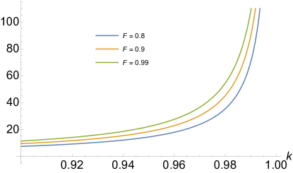
Figure 3: Ratio between $n_{\mathrm{max}}$’s sensitivity to $k$ and sensitivity to $F$, i.e. $S_{k}/S_{F}$. For this figure $d=3$ is fixed.

III.3 Comparison with local imperfect GHZ state

We have considered the global sensing strategy with imperfect initial $d$-qubit entanglement across the $d$ sensor nodes, together with imperfect local entanglement generation when extending the $d$-qubit probe state to the $nd$-qubit state. If we take into account imperfect local entanglement generation, it is natural to consider that the comparison baseline, the local strategy, will also need to utilize imperfect local entangled probe state.

We consider a specific local strategy, where each node will utilize $n$-qubit imperfect GHZ state to probe the single local parameter which is encoded through coupling with the $Z$ component of the collective spin. In such single-parameter estimation scenario for each node, the QFI be calculated through [57]:

$$F_{\rho_{0},H}= 2\sum_{a,b}\frac{(\lambda_{a0}-\lambda_{b0})^{2}}{\lambda_{a0}+\lambda_{b0}}|\langle\psi_{a0}|H|\psi_{b0}\rangle|^{2}$$

$$= 2\sum_{a,b}(\lambda_{a0}+\lambda_{b0})|\langle\psi_{a0}|H|\psi_{b0}\rangle|^{2}-\sum_{a,b}\frac{8\lambda_{a0}\lambda_{b0}}{\lambda_{a0}+\lambda_{b0}}|\langle\psi_{a0}|H|\psi_{b0}\rangle|^{2},$$ (50)

where $\lambda_{a0}$ are eigenvalues of local initial probe state $\rho_{0}=\sum_{a}\lambda_{a0}|\psi_{a0}\rangle\langle\psi_{a0}|$, and $H=\frac{1}{2}\sum_{i=0}^{n-1}\sigma^{(i)}_{z}$ is the local generator of the parameter-encoding unitary. Similar to the previous twirling argument, here without loss of generality, we consider local initial probe state to be in the form of GHZ-diagonal state. Then through analysis that is same to the multiparameter QFIM case, we can arrive at the analytical form of QFI for initial GHZ-state diagonal state which is identical to the QFIM in multiparameter case:

$$\mathcal{F}=n^{2}-n^{2}\sum_{(a,b)\in\mathcal{S}}\frac{2\lambda_{a0}\lambda_{b0}}{\lambda_{a0}+\lambda_{b0}}=(1-C)n^{2},$$ (51)

where $\mathcal{S}$ is again the set of index pairs $(a,b)$ such that $|\psi_{a0}\rangle$ and $|\psi_{b0}\rangle$ are superpositions of the same two computational basis states but with opposite relative phase, and we re-emphasize that for such pairs both $(a,b)$ and $(b,a)$ are included in $\mathcal{S}$.

We focus on the impact of imperfect initial probe state preparation, and thus assume that the optimal measurement on each local node can be performed, that is the QCRB for each sensor node’s local estimation can be achieved. Then according to the propagation of error, we have the estimation error for the average of all local parameters with the local strategy:

$$\mathrm{Var}_{\mathrm{local}}(\hat{\theta}_{1})= \sum_{l=1}^{d}\left(\frac{\partial\theta_{1}}{\partial x_{l}}\right)^{2}\mathrm{Var}(\hat{x}_{l})=\frac{1}{n^{2}N}\sum_{l=1}^{d}\frac{1}{d(1-C_{l})},$$ (52)

for $N$ repetitions of measurements, $d$ sensor nodes, and $n$ qubits per node.

We consider the following model of imperfect local entanglement generation: The generated local probe state at each node is an identical depolarized GHZ state with fidelity $F(n)=\tilde{k}^{n-1}$ as a function of the number of local sensors $n$, where $\tilde{k}\in(0,1)$ is a constant representing the quality of local entanglement generation and the higher the better. To make the comparison with the global strategy, we consider the following correspondence: $\tilde{k}=\sqrt[d]{k}$, where $k$ is the same constant as we used for the fidelity of the $nd$-qubit global probe state with imperfect local entanglement generation. This correspondence is motivated by the fact that when $n$ increases one, $d$ qubits are added to the global probe state, while only one qubit is added to each node’s local probe state. Given this model, we can further express $\mathrm{Var}_{\mathrm{local}}(\hat{\theta}_{1})$ as:

$$\mathrm{Var}_{\mathrm{local}}(\hat{\theta}_{1})=\frac{1}{(1-C_{\mathrm{local}})n^{2}N},$$ (53)

where

$$C_{\mathrm{local}}(d,n,k)=\frac{\left(1-k^{(n-1)/d}\right)\left[(2^{n}-2)k^{1/d}+4^{n}k^{n/d}\right]}{(2^{n}-1)\left[k^{1/d}+(2^{n}-2)k^{n/d}\right]}.$$ (54)

Then we can make the explicit comparison between $\eta_{\mathrm{global}}=d[1-C_{\mathrm{dp}}(F,d,n,k)]$ for the global strategy and $\eta_{\mathrm{local}}=(1-C_{\mathrm{local}})$ for the local strategy. As an example, we visualize the ratio $r=\eta_{\mathrm{global}}/\eta_{\mathrm{local}}$ when $F=0.9$, $d=3$, and $k=0.9999$, in Fig. 4. It can be observed that the threshold of local sensor number for advantage over imperfect local strategy is higher than the threshold for advantage over the optimal local strategy. This is intuitive as the baseline in the former scenario is worse. However, it is important to re-emphasize that the global strategy performance will become worse than the specific local strategy, even if imperfect local entanglement generation is included in the local strategy. This reinforces the fundamental limit in the advantage of global strategy when local entanglement generation is imperfect. In fact, this can be seen analytically through the asymptotic analysis of $\eta_{\mathrm{local}}$ and $\eta_{\mathrm{global}}$ (under the reasonable assumption of $1>k>1/2$):

$$\eta_{\mathrm{global}}\sim (dF)k^{n-1},$$ (55)

$$\eta_{\mathrm{local}}\sim \left(k^{1/d}\right)^{n-1},$$ (56)

which means that as $n$ increases $\eta_{\mathrm{global}}$ will always drop below $\eta_{\mathrm{local}}$.

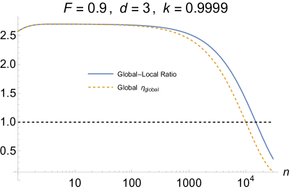
Figure 4: Visualization of the comparison between global and local sensing strategies with imperfect local entanglement generation, when $F=0.9$, $d=3$, and $k=0.9999$. The blue solid line denotes $r=\eta_{\mathrm{global}}/\eta_{\mathrm{local}}$, and the yellow dashed line denotes $\eta_{\mathrm{global}}$, which is identical to $\eta_{\mathrm{dp}}$ in the main text. The black dashed line marks the baseline value of 1: If $\eta_{\mathrm{global}}>1$ there is quantum advantage over the optimal local strategy, and if $r>1$ there is advantage of using global strategy over local strategy when local entanglement generation is imperfect for both.

IV Local measurement for entangled sensors

According to propagation of error, we can obtain the variance of estimating a certain parameter encoded in a quantum state from the measurement results of an observable $M$ [57]:

$$\mathrm{Var}_{M}(\hat{\theta}_{1})=\frac{\langle M^{2}\rangle-\langle M\rangle^{2}}{\left|\frac{\partial}{\partial\theta_{1}}\langle M\rangle\right|^{2}},$$ (57)

where the expectation value $\langle M\rangle$ is taken under the encoded state $\rho_{x}$ and thus is a function of local parameters $x_{i}$. We note that in quantum sensing, the values of parameters to estimate are usually small. Therefore, when using the propagation of error formula we may take the limit of $\theta\rightarrow 0$. It is straightforward to use the aforementioned orthogonal transformation to convert $x_{i}$ into linear combinations of derived parameters that include the parameter of interest $\theta_{1}$. Gram-Schmidt process can be used to construct orthonormal basis which includes $v_{1}=(1,\dots,1)^{T}/\sqrt{d}$. For instance, for $d=3$ we can construct an orthonormal basis:

$$v_{1}=(1,1,1)^{T}/\sqrt{3},$$ (58)

$$v_{2}=(-1,2,-1)^{T}/\sqrt{6},$$ (59)

$$v_{3}=(-1,0,1)^{T}/\sqrt{2},$$ (60)

where $\theta_{i}=v_{i}^{T}x$, and in our scenario we are only interested in $\theta_{1}$. Given a specific $d$-dimensional orthonormal basis, we will be able to transform the $x$-dependence of $\langle M\rangle$ into $\theta$-dependence. Then the partial derivative with respect to $\theta_{1}$ will be straightforward.

IV.1 Optimal measurement for noiseless case is useless for noisy case

Recall that here the observable of our interest is $M=\sigma_{x}^{\otimes nd}$. For GHZ-diagonal states in general, the expectation value of observable is the average of expectation value under pure GHZ states weighted by the diagonal elements of density matrix in GHZ basis. Since $M^{2}=I^{\otimes nd}$ we always have $\langle M^{2}\rangle=1$. Consider GHZ states corresponding to the same binary string but with opposite relative phase $|\mathrm{GHZ}_{nd}^{\pm}(b)\rangle=(|b\rangle\pm|2^{nd}-b-1\rangle)/\sqrt{2}$, where $|x\rangle$ denote the computational basis state corresponding to the binary representation of integer $x=0,1,\dots,2^{nd}-1$ and $b=0,1,\dots,2^{nd-1}-1$. We have that:

$$\langle\mathrm{GHZ}_{nd}^{+}(b)|U^{\dagger}(x)MU(x)|\mathrm{GHZ}_{nd}^{+}(b)\rangle= \frac{1}{2}\left(\langle b|+e^{-i\phi(x)}\langle 2^{nd}-b-1|\right)\sigma_{x}^{\otimes nd}\left(|b\rangle+e^{i\phi(x)}|2^{nd}-b-1\rangle\right)$$

$$= \frac{1}{2}\left(e^{i\phi(x)}\langle b|\sigma_{x}^{\otimes nd}|2^{nd}-b-1\rangle+e^{-i\phi(x)}\langle 2^{nd}-b-1|\sigma_{x}^{\otimes nd}|b\rangle\right)$$

$$= \frac{1}{2}\left(e^{i\phi(x)}+e^{-i\phi(x)}\right)=\cos\left(\phi(x)\right)$$

$$= -\langle\mathrm{GHZ}_{nd}^{-}(b)|U^{\dagger}(x)MU(x)|\mathrm{GHZ}_{nd}^{-}(b)\rangle$$ (61)

Given the above properties of GHZ-diagonal state under the encoding channel and observable of our interest, the analysis of depolarized GHZ state becomes significantly simplified. Only $(|0\dots 0\rangle\pm|1\dots 1\rangle)/\sqrt{2}$ contribute to the expectation value $\langle M\rangle$, because other GHZ states corresponding to the same binary string have identical weights and thus their contributions cancel each other. Thus for depolarization error model we have:

$$\langle M\rangle_{n}(\theta_{1})=\left(F-\frac{1-F}{2^{nd}-1}\right)\cos\left(n\sqrt{d}\theta_{1}\right),$$ (62)

where $n$ denotes the number of sensors per node, and noiseless local entanglement generation corresponds to $n=1$. Then we can substitute the above into Eqn. 57:

$$\mathrm{Var}_{M}(\hat{\theta}_{1})=\frac{1-\left(F-\frac{1-F}{2^{nd}-1}\right)^{2}\cos^{2}\left(n\sqrt{d}\theta_{1}\right)}{dn^{2}\left(F-\frac{1-F}{2^{nd}-1}\right)^{2}\sin^{2}\left(n\sqrt{d}\theta_{1}\right)}$$ (63)

It is obvious that when taking the above function to the limit of $\theta_{1}\rightarrow 0$ it goes to infinity if $F<1$, which suggests that this specific measurement scheme is useless to estimate small values with high accuracy. We comment that the divergence of estimation variance in small local parameter regime is general for any GHZ-diagonal state with fidelity below 1, because the denominator in error propagation formula will approach zero, while the numerator will stay non-zero when the fidelity is not equal to 1.

IV.2 Optimization of restricted local measurement

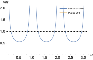
Figure 5: The estimation variance as a function of azimuthal angle $\alpha$ is shown as the blue solid curve, for $F=0.8,d=3,n=1$. The black dashed line denotes the baseline which can be achieved by the best local strategy. The yellow solid line demonstrates the inverse of the QFI, representing the ultimate estimation variance which requires some other measurement.

The space of local measurement schemes is large. For concreteness and simplicity, here we focus on a specific family of measurement characterized by one parameter $\alpha$: $M(\alpha)=\left[O(\alpha)\right]^{\otimes nd}$ where $O(\alpha)=|\psi^{+}(\alpha)\rangle\langle\psi^{+}(\alpha)|-|\psi^{-}(\alpha)\rangle\langle\psi^{-}(\alpha)|$ with $|\psi^{\pm}(\alpha)\rangle=(|0\rangle\pm e^{i\alpha}|1\rangle)$. That is, $O(\alpha)=e^{i\alpha}|1\rangle\langle 0|+e^{-i\alpha}|0\rangle\langle 1|$ while the optimal measurement in noiseless case is $M(0)$. Notice that $\left(O(\alpha)\right)^{2}=I$ and $O(\alpha)$ is always off-diagonal in computational basis. Thus we can still simplify its expectation values under GHZ-diagonal states, especially depolarized GHZ states with $nd$ qubits:

$$\mathrm{Var}_{M(\alpha)}(\hat{\theta}_{1})=\frac{1-\left(F-\frac{1-F}{2^{nd}-1}\right)^{2}\cos^{2}\left[n\sqrt{d}(\theta_{1}+\sqrt{d}\alpha)\right]}{dn^{2}\left(F-\frac{1-F}{2^{nd}-1}\right)^{2}\sin^{2}\left[n\sqrt{d}(\theta_{1}+\sqrt{d}\alpha)\right]}.$$ (64)

It is clear that the non-zero azimuthal angle $\alpha$ has the effect of modifying the undesired zero denominator when $\theta_{1}=0$. Then we can safely take $\theta_{1}=0$ and optimize $\alpha$:

$$\left.\mathrm{Var}_{M(\alpha)}(\hat{\theta}_{1})\right|_{\theta_{1}=0}=\frac{1-\left(F-\frac{1-F}{2^{nd}-1}\right)^{2}\cos^{2}\left(nd\alpha\right)}{dn^{2}\left(F-\frac{1-F}{2^{nd}-1}\right)^{2}\sin^{2}\left(nd\alpha\right)}.$$ (65)

The partial derivative with respect to $\alpha$ gives rise to:

$$\frac{\partial}{\partial\alpha}\left.\mathrm{Var}_{M(\alpha)}(\hat{\theta}_{1})\right|_{\theta_{1}=0}=-\frac{2^{nd+1}(1-F)\left[2^{nd}(1+F)-2\right]}{n\left(2^{nd}F-1\right)^{2}}\frac{\cos(nd\alpha)}{\sin^{3}(nd\alpha)}.$$ (66)

It is thus obvious that the variance takes the minimum values when $\cos(nd\alpha_{\mathrm{opt}})=0$, i.e. $\alpha_{\mathrm{opt}}=\frac{2l+1}{2nd}\pi$ with $l\in\mathbb{Z}$. The minimum value is:

$$\left.\mathrm{Var}_{M(\alpha_{\mathrm{opt}})}(\hat{\theta}_{1})\right|_{\theta_{1}=0}=\frac{1}{d\left(F-\frac{1-F}{2^{nd}-1}\right)^{2}n^{2}}=\frac{1}{\eta_{M(\alpha_{\mathrm{opt}})}n^{2}}.$$ (67)

Such periodicity of the optimal azimuthal angle echoes with previous numerical results [65]. We can visualize the parameter estimation variance with different $\alpha$ for $n=1$ in Fig. 5. The ratio between $\eta_{M(\alpha_{\mathrm{opt}})}$ and $\eta_{\mathrm{dp}}(k=1)$ is:

$$\frac{\eta_{M(\alpha_{\mathrm{opt}})}}{\eta_{\mathrm{dp}}(k=1)}=F+\frac{1-F}{2^{nd}-1},$$ (68)

which quickly converges to $F$ for larger $n$ and $d$. The fidelity threshold for $nd$-qubit depolarized GHZ state to be advantageous over the optimal local strategy when using the optimized azimuthal measurement is given by $\eta_{M(\alpha_{\mathrm{opt}})}=1$:

$$F_{\mathrm{th},M(\alpha_{\mathrm{opt}})}(n)=\frac{2^{nd}+\sqrt{d}-1}{2^{nd}\sqrt{d}}.$$ (69)

For $n=1$, we have the fidelity threshold for the initial depolarized GHZ state to demonstrate advantage when using the optimized azimuthal measurement, i.e. $\eta_{M(\alpha_{\mathrm{opt}})}>1$:

$$F_{\mathrm{th},M(\alpha_{\mathrm{opt}})}(1)=\frac{2^{d}+\sqrt{d}-1}{2^{d}\sqrt{d}},$$ (70)

which can be easily shown to be monotonically decreasing for the distributed regime $d\geq 2$ of our interest.

We re-emphasize that our optimization of the azimuthal measurement is not a global optimization, as it is locally separable when there are multiple sensor qubits per node. In principle we could utilize entangling measurement locally. However, the fact that when $n=1$ the optimized azimuthal measurement could not saturate the QCRB implies that the QCRB for this distributed quantum sensing problem is not achievable with local measurement. It is known that the QCRB can be achieved by projective measurement, and when $n=1$ the local projective measurement should be a tensor product of single-qubit projective measurements. Moreover, the assumed depolarization noise on the GHZ state guarantees symmetry among all qubits, so it suffices to consider identical projective measurement per qubit. Note that under our problem setup, z-direction projection is unable to extract the information of the parameter to estimate. Therefore, our optimization of azimuthal projective measurement should have covered the optimal local measurement, while as seen in the results they could not achieve the QCRB. On the other hand, suppose we insist on applying the global entangling measurement, it will need distribution of additional entangled state by the quantum network as resource to implement the measurement. Consequently, the performance of parameter estimation will be further limited by the fidelity of resource state for performing entangling measurement, and thus the fidelity of distributed entangled state by the network must be high. However, as we have seen that when the network is able to distributed high fidelity entangled state, performing local optimized azimuthal measurement can already achieve fairly low estimation variance, which is only $\sim 1/F$ times the ultimate achievable variance by the globally optimal measurement.

IV.2.1 Comment on rank-2 dephased GHZ state

We can also consider the azimuthal measurement for the $d$-qubit, i.e. $n=1$, rank-2 dephased GHZ state $\rho=F|\mathrm{GHZ}_{d}\rangle\langle\mathrm{GHZ}_{d}|+(1-F)Z|\mathrm{GHZ}_{d}\rangle\langle\mathrm{GHZ}_{d}|Z$. Then in the small parameter regime $\theta_{1}\rightarrow 0$, the parameter estimation variance as a function of the azimuthal angle $\alpha$ is:

$$\left.\mathrm{Var}_{M(\alpha),r=2}(\hat{\theta}_{1})\right|_{\theta_{1}=0}=\frac{1-\left(2F-1\right)^{2}\cos^{2}\left(d\alpha\right)}{d\left(2F-1\right)^{2}\sin^{2}\left(d\alpha\right)}.$$ (71)

Then we can take the partial derivative with respect to $\alpha$ to perform optimization:

$$\frac{\partial}{\partial\alpha}\left.\mathrm{Var}_{M(\alpha),r=2}(\hat{\theta}_{1})\right|_{\theta_{1}=0}=-\frac{8F(1-F)}{(2F-1)^{2}}\frac{\cos(d\alpha)}{\sin^{3}(d\alpha)}.$$ (72)

Therefore, the lowest variance is achieved when $\cos(d\alpha_{\mathrm{opt}})=0$, i.e. $\alpha_{\mathrm{opt}}=\frac{2l+1}{2d}\pi$ with $l\in\mathbb{Z}$, and this condition is exactly the same for the depolarized GHZ state with $n=1$. Then the minimal variance is:

$$\left.\mathrm{Var}_{M(\alpha_{\mathrm{opt}}),r=2}(\hat{\theta}_{1})\right|_{\theta_{1}=0}=\frac{1}{d(2F-1)^{2}}=\frac{1}{\mathcal{F}}.$$ (73)

This result means that the optimal azimuthal measurement is able to saturate the QCRB for rank-2 dephased GHZ state.

IV.3 Bell state fidelity requirement estimation

Moreover, we can estimate the fidelity requirement of bipartite entanglement (Bell pair) distribution network to achieve quantum advantage in the local parameter average estimation task, by taking the $(d-1)$-th root of the fidelity threshold. This estimation comes from the assumption that we need $(d-1)$ bipartite entangled states between the sensor nodes to assemble the desired $d$-qubit GHZ state, and the approximation that the final GHZ state has fidelity equal to the product of all Bell states’ fidelities. Specifically, for $n=1$ we have:

$$F_{\mathrm{th},M(\alpha_{\mathrm{opt}})}^{\mathrm{Bell}}=\left(\frac{2^{d}-1+\sqrt{d}}{2^{d}\sqrt{d}}\right)^{\frac{1}{d-1}},$$ (74)

$$F_{\mathrm{th,opt}}^{\mathrm{Bell}}=\left(2^{-d}+\frac{(2^{d}-1)\left(2^{d}-2+\sqrt{(2^{d}-2)^{2}+2^{d+3}d}\right)}{2^{2d+1}d}\right)^{\frac{1}{d-1}},$$ (75)

where we use the superscript “Bell” to emphasize that the above fidelity thresholds are for Bell states distributed by the quantum network. The two thresholds are visualized in Fig. 6(a). It can be seen that the fidelity threshold for the global optimal measurement slightly decreases when the number of sensor nodes $d$ is small. More specifically, we have:

$$F_{\mathrm{th,opt}}^{\mathrm{Bell}}(2)\approx 0.730,~{}F_{\mathrm{th,opt}}^{\mathrm{Bell}}(3)\approx 0.714,~{}F_{\mathrm{th,opt}}^{\mathrm{Bell}}(4)\approx 0.711,$$

$$F_{\mathrm{th,opt}}^{\mathrm{Bell}}(5)\approx 0.716,~{}F_{\mathrm{th,opt}}^{\mathrm{Bell}}(6)\approx 0.726,~{}F_{\mathrm{th,opt}}^{\mathrm{Bell}}(7)\approx 0.738.$$ (76)

Nevertheless, in general both the thresholds increase monotonically as the number of sensor nodes increases. Moreover, we can straightforwardly evaluate the asymptotic scaling of both thresholds:

$$F_{\mathrm{th},M(\alpha_{\mathrm{opt}})}^{\mathrm{Bell}}\sim d^{\frac{1}{2(1-d)}},$$ (77)

$$F_{\mathrm{th,opt}}^{\mathrm{Bell}}\sim d^{\frac{1}{1-d}}.$$ (78)

Very curiously, the Bell state fidelity threshold for the global optimal measurement is the square of the threshold for the optimized azimuthal measurement in the asymptotic limit of $d\rightarrow\infty$, i.e. $F_{\mathrm{th,opt}}^{\mathrm{Bell}}\sim\left(F_{\mathrm{th},M(\alpha_{\mathrm{opt}})}^{\mathrm{Bell}}\right)^{2}$. It is then easily seen that both fidelity thresholds converge to one in the large $d$ limit. To visualize the asymptotic scaling, we further plot the thresholds of infidelity $\epsilon=1-F$ in log-log coordinate in Fig. 6(b). It is clear that $\epsilon_{\mathrm{th,opt}}^{\mathrm{Bell}}/2$ is almost equal to $\epsilon_{\mathrm{th},M(\alpha_{\mathrm{opt}})}^{\mathrm{Bell}}$ when $d$ becomes large, which verifies the quadratic relation of the asymptotic scalings.

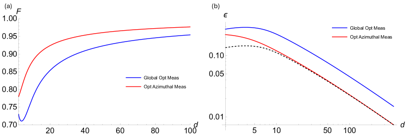
Figure 6: Estimation of Bell state fidelity thresholds for demonstrating quantum advantage in distributed quantum sensing, where the initial $d$-qubit GHZ state is assembled from $(d-1)$ Bell states distributed by the quantum network. (a) The Bell state fidelity threshold when the global optimal measurement is allowed is depicted by the blue curve, while the threshold when only the optimized azimuthal measurement can be performed is illustrated by the red curve. (b) The infidelity $\epsilon=1-F$ thresholds were plotted in the log-log coordinate for additional visualization insight. The blue curve again corresponds to the global optimal measurement and the red curve to the optimized azimuthal measurement. For reference, we plot the half of the infidelity threshold for the global optimal measurement in black dashed line, to better demonstrate the relationship between the asymptotic scalings of both thresholds.

V Parameter estimation with failure in entanglement distribution

In practical quantum networks, there is always non-zero probability to fail in the generation of the demanded entangled state. In our multiparameter estimation scenario where we want to estimate the average of all local parameters, and the probe state we want is a $d$-qubit GHZ state that entangles all $d$ sensor nodes. The state is generated through assembling bipartite entangled states distributed by the quantum network. What might happen is that some bipartite entangled states are not successfully generated within certain attempts.

V.1 Hybrid strategy

We consider a specific way of bipartite entangled state assembly to generate the GHZ state: We assume there is a center node, which will share bipartite entanglement with other nodes. Therefore, for the nodes which fail to establish entangled link with the center node, they will remain separable from other nodes, while all the nodes that successfully share entangled link with the center node will be entangled together. Let $\mathcal{N}$ s.t. $|\mathcal{N}|=d$ be the index set of all sensor noes, and $\mathcal{C}$ be the index set for the nodes which remain isolated, thus the set difference $\mathcal{N}\setminus\mathcal{C}$ denotes the index set of nodes that will be entangled. For the objective parameter to estimate $\theta_{1}=\sum_{i\in\mathcal{N}}x_{i}/\sqrt{d}$, it can be rewritten as:

$$\theta_{1}= \frac{1}{\sqrt{d}}\sum_{i\in\mathcal{C}}x_{i}+\sqrt{\frac{|\mathcal{N}\setminus\mathcal{C}|}{d}}\left(\frac{1}{\sqrt{|\mathcal{N}\setminus\mathcal{C}|}}\sum_{j\in\mathcal{N}\setminus\mathcal{C}}x_{j}\right)$$

$$= \frac{1}{\sqrt{d}}\sum_{i\in\mathcal{C}}x_{i}+\sqrt{\frac{|\mathcal{N}\setminus\mathcal{C}|}{d}}\theta^{\prime}_{1},$$ (79)

where the second term is proportional to the average of local parameters on all the nodes that are entangled, $\theta^{\prime}_{1}$. When not all sensor nodes are entangled, we consider that the sensor network will use the following hybrid strategy: The isolated nodes use local probe state to estimate the local parameters $x_{i},i\in\mathcal{C}$ individually, while the entangled nodes use a globally entangled probe state to estimate $\theta^{\prime}_{1}$. Then according to propagation of errors, we have the variance of estimating $\theta$ by such a hybrid strategy as:

$$\mathrm{Var}_{\mathrm{hybrid}}(\hat{\theta}_{1,\mathcal{C}})=\frac{1}{d}\sum_{i\in\mathcal{C}}\mathrm{Var}(\hat{x}_{i})+\frac{|\mathcal{N}\setminus\mathcal{C}|}{d}\mathrm{Var}(\hat{\theta}^{\prime}_{1}),$$ (80)

where the subscript $\mathcal{C}$ for estimator $\hat{\theta}_{1,\mathcal{C}}$ emphasizes that the estimator is uniquely determined by $\mathcal{C}$. We may also call $\mathcal{C}$ a configuration.

V.2 Combining different configurations

Due to the probabilistic nature of remote entanglement distribution over the quantum repeater networks under our consideration, for each attempt of probe state generation the configuration $\mathcal{C}$ can be different. Therefore, when we repeat the quantum sensing cycles for many shots to accumulate statistical data, the data may correspond to different configurations, and moreover, we know the correspondence exactly due to the heralded nature of quantum repeater network protocols. Let $\mathfrak{C}$ denotes the collection of all possible configurations $\mathcal{C}$. For the scenario with $d$ sensor nodes, we have that $|\mathfrak{C}|=\sum_{n=0}^{d-2}\binom{d}{n}+1=2^{d}-d$ without over-counting, because when $|\mathcal{C}|=d-1$ it is equivalent to that all nodes are isolated.

We would like to utilize all data to increase the estimation accuracy. Suppose we repeat the quantum sensing cycle for $N$ times so that we have $N$ data points, and each configuration $\mathcal{C}$ occurs with probability $p_{\mathcal{C}}$. That is, we may expect that there are $N_{\mathcal{C}}=p_{\mathcal{C}}N$ data points corresponding to configuration $\mathcal{C}$, then we have $\mathrm{Var}(\hat{\theta}_{1,\mathcal{C}})\propto 1/N_{\mathcal{C}}$. Given the assumption of (locally) unbiased estimators, we know that the normalized linear combination of $\hat{\theta}_{1,\mathcal{C}}$ still has the mean of $\theta_{1}$. Then our objective is to minimize the variance of the normalized linear combination:

$$\hat{\theta}_{1}=\sum_{\mathcal{C}\in\mathfrak{C}}w_{\mathcal{C}}\hat{\theta}_{1,\mathcal{C}},~{}\mathrm{s.t.}~{}\sum_{\mathcal{C}}w_{\mathcal{C}}=1.$$ (81)

We may further assume that $\hat{\theta}_{1,\mathcal{C}}$ are uncorrelated, which according to the Bienaymé’s identity gives us:

$$\mathrm{Var}(\hat{\theta}_{1})=\sum_{\mathcal{C}\in\mathfrak{C}}w_{\mathcal{C}}^{2}\mathrm{Var}(\hat{\theta}_{1,\mathcal{C}}).$$ (82)

Then it can be derived using Lagrange multiplier that the optimal weighting for the minimum variance is:

$$w_{\mathcal{C}}=\frac{1}{\mathrm{Var}(\hat{\theta}_{1,\mathcal{C}})}\left[\sum_{\mathcal{C}\in\mathfrak{C}}\frac{1}{\mathrm{Var}(\hat{\theta}_{1,\mathcal{C}})}\right]^{-1},$$ (83)

which is the so-called inverse-variance weighting that gives the minimum variance:

$$\mathrm{Var}_{\mathrm{min}}(\hat{\theta}_{1})= \sum_{\mathcal{C}\in\mathfrak{C}}\frac{1}{\mathrm{Var}^{2}(\hat{\theta}_{1,\mathcal{C}})}\left[\sum_{\mathcal{C}\in\mathfrak{C}}\frac{1}{\mathrm{Var}(\hat{\theta}_{1,\mathcal{C}})}\right]^{-2}\mathrm{Var}(\hat{\theta}_{1,\mathcal{C}})=\left[\sum_{\mathcal{C}\in\mathfrak{C}}\frac{1}{\mathrm{Var}(\hat{\theta}_{1,\mathcal{C}})}\right]^{-1}.$$ (84)

We comment that when the problem scale $d$ increases, the size of configuration space $\mathfrak{C}$ increases exponentially. Therefore, the minimization of estimation variance by combining the data from all possible configurations will become practically impossible eventually if the problem scale is large. However, when the quantum repeater network is low loss and low error, it is almost guaranteed that every attempt of probe state generation will succeed with a $d$-qubit GHZ state. In such cases, it is good enough to use only the data points which correspond to a complete $d$-qubit GHZ state to estimate $\theta_{1}$.

On the other hand, we may coarse grain the configurations to account only the number of nodes which are entangled for approximation. Thus the corresponding GHZ states are the ensemble average of the GHZ states in different configurations. Let $\mathfrak{C}_{n}$ denote the collection of $\mathcal{C}$ s.t. $|\mathcal{C}|=n$, where $n=0,1,\dots,d-2,d$. Specifically, we consider that $\mathrm{Var}(\hat{\theta}_{1,\mathcal{C}})=F_{\mathcal{C}}/N_{\mathcal{C}}$. In this way, we have the approximate minimum variance:

$$\mathrm{Var}_{\mathrm{min}}(\hat{\theta}_{1})= \left[\sum_{\mathcal{C}\in\mathfrak{C}}\frac{1}{\mathrm{Var}(\hat{\theta}_{1,\mathcal{C}})}\right]^{-1}=\left[\sum_{\mathcal{C}\in\mathfrak{C}}\frac{N_{\mathcal{C}}}{F_{\mathcal{C}}}\right]^{-1}$$

$$= \left[\frac{N_{d}}{F_{d}}+\sum_{n=0}^{d-2}\sum_{\mathcal{C}\in\mathfrak{C}_{n}}\frac{N_{\mathcal{C}}}{F_{\mathcal{C}}}\right]^{-1}$$

$$\approx \left[\frac{N_{d}}{F_{d}}+\sum_{n=0}^{d-2}\frac{\sum_{\mathcal{C}\in\mathfrak{C}_{n}}N_{\mathcal{C}}}{F_{n}}\right]^{-1}=\left[\frac{N_{d}}{F_{d}}+\sum_{n=0}^{d-2}\frac{N_{n}}{F_{n}}\right]^{-1},$$ (85)

where $F_{n}$ denotes the coefficient of variance for configurations with $n$ isolated nodes, and $N_{n}$ denotes the total number of data points for configurations with $n$ isolated nodes.

VI Probe state assembly from bipartite entanglement for DQS

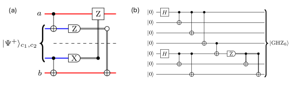
Figure 7: Circuits of (a) CNOT teleportation and (b) GHZ merging. The standard GHZ generation circuit is included in the GHZ merging circuit as the first part.

The preparation of the initial probe state for DQS is envisioned to be based on bipartite entanglement distributed between sensor nodes by quantum networks. Sensor nodes will perform local operations and classical communication (LOCC) to create multipartite entangled state across themselves as the probe state. In this section, we describe two methods to do so, namely gate teleportation and GHZ merging. Before going into details, we comment that in practice the quantum networks might be hybrid, in that different functions are realized by different physical systems. For instance, communication qubits which are in charge of generating and distributing entanglement might be different from the quantum sensors used for DQS. Therefore, to make DQS a reality, experimental development of quantum interconnects [110, 111] is indispensable.

VI.1 Gate teleportation

A Bell pair can be used to perform CNOT teleportation, and the circuit of CNOT teleportation is shown in Fig. 7(a). Then we can directly run the standard GHZ generation circuit, assuming the availability of two-qubit gates between communication qubits and sensor qubits. The standard GHZ generation circuit is shown in the first part of Fig. 7(b).

We can estimate the resources needed for this approach. All generated Bell pairs are consumed, and thus to generate probe state of size $N$, $N$ other sensor qubits (one of them is the center) need to be initialized when performing CNOT teleportation. According to GHZ state generation circuit, in total $(N-1)$ CNOTs are needed, equal to $(N-1)$ Bell pairs. During each gate teleportation after two single qubit measurements, (in ideal case) there are 1/4 probability that no local unitary correction is needed, 1/2 probability that one local unitary correction is needed, and 1/4 probability that two local unitary corrections are needed. Moreover, the two single qubit measurements are in different basis, observing that the physical implementation of (matter) qubit measurement is usually only native in one basis, we may consider that an additional single-qubit unitary is needed to transform measurement basis. Therefore, to generate $N$-qubit GHZ state in quantum networks based on gate teleportation: $(3N-2)$ qubits are needed, $(2N-2)$ of which are dedicated to $(N-1)$ Bell pairs; $(2N-2)$ single-qubit measurements are needed; $(2N-2)$ local CNOTs are needed; and on average $(N-1)$ (or $(2N-2)$) single-qubit gates are needed. The estimation is summarized in Table. 2.

VI.2 GHZ merging

Merging of two GHZ states can be achieved with local CNOT and measurement feedforward, as shown explicitly in the following where we consider the merging of two GHZ states with $N$ and $M$ qubits, respectively:

$$|\mathrm{GHZ}_{N}\rangle|\mathrm{GHZ}_{M}\rangle\propto(|\underbrace{0\dots 0}_{N\times~{}0}\rangle+|\underbrace{1\dots 1}_{N\times~{}1}\rangle)(|\underbrace{0\dots 0}_{M\times~{}0}\rangle+|\underbrace{1\dots 1}_{M\times~{}1})\rangle$$ (86)

$$\xrightarrow[]{\mathrm{CNOT}_{N,N+1}} (|\underbrace{0\dots 0}_{(N-1)\times~{}0}00\underbrace{0\dots 0}_{(M-1)\times~{}0}\rangle+|\underbrace{0\dots 0}_{(N-1)\times~{}0}01\underbrace{1\dots 1}_{(M-1)\times~{}1}\rangle+|\underbrace{1\dots 1}_{(N-1)\times~{}1}11\underbrace{0\dots 0}_{(M-1)\times~{}0}\rangle+|\underbrace{1\dots 1}_{(N-1)\times~{}1}10\underbrace{1\dots 1}_{(M-1)\times~{}1}\rangle).$$

Then it is obvious that if we measure the target qubit of CNOT (with index $N+1$ when all qubits are indexed from 1 through $N+M$) in computational basis, when the measurement outcome is 0, the post-measurement state is exactly a GHZ state with $N+M-1$ qubits, and when the outcome is 1, the post-measurement state can be transformed into a GHZ state with $N+M-1$ qubits by applying $\min[N,M-1]$ local X gates to flip the $|0\rangle$ and $|1\rangle$. An example circuit of GHZ merging is visualized in Fig. 7(b).

We can also estimate the resources needed for this approaches. Different from using gate teleportation, merging does not consume all qubits in generated Bell pairs. We need to perform $(N-1)$ mergings, and for each merging there is 1/2 probability that one local unitary correction is needed, and 1/2 probability that no local unitary correction is needed. Therefore, to generate $N$-qubit GHZ state in quantum networks based on merging: $(2N-2)$ qubits are needed, all of which are dedicated to $(N-1)$ Bell pairs; $(N-1)$ single-qubit measurements are needed; $(N-1)$ local CNOTs are needed; and on average $(N-1)/2$ single-qubit gates are needed. The estimation is summarized in Table. 2.

However, consider the separation between communication qubits and sensor qubits, we need to first generate the GHZ states across communication qubits from merging and then perform local SWAP gates to swap the GHZ state from communication qubits to the sensor qubits. In this case, we need $N$ sensor qubits, and $N$ local SWAP gate between communication and sensor qubits (which can be decomposed into 3 CNOTs).

Table 2: Resource estimation for $N$-qubit GHZ state assembly from $(N-1)$ Bell pairs by CNOT teleportation and GHZ merging.

	qubits	1-qubit measurements	2-qubit gates	1-qubit gates
CNOT teleportation	$3N-2$	$2N-2$	$2N-2$	$N-1$
GHZ merging	$2N-2$	$N-1$	$N-1$	$(N-1)/2$

VII Network simulation details

In this section we provide details of how we simulate the initial probe state preparation for DQS using SeQUeNCe.

VII.1 Entanglement distribution

The preparation of multipartite entangled probe state starts with the distribution of bipartite entangled states between pairs of network nodes. These bipartite entangle states will be assembled into multipartite entangled states using local operations and classical communication, such as gate teleportation and GHZ state merging (graph state fusion).

The distribution of bipartite entanglement involves remote entanglement generation between nearest network nodes that are directly connected by a physical implementation of quantum channels (e.g., optical fibers or free-space optics), entanglement swapping which extends the generated entangled states to more distant node pairs, and potentially entanglement purification which is expected to improve the quality (fidelity) of distributed entangled pairs.

For entanglement generation, in SeQUeNCe we implement a new abstract model of single-heralded entanglement generation protocol based on meet-in-the-middle photonic Bell state measurement. The underlying processes assumed for a single attempt of entanglement generation includes:

1. Local memory-photon entanglement on a network node is generated, and the photon is transmitted to a middle interference center via a lossy optical fiber to perform heralded measurement (Bell state measurement/BSM).

2. Two photons being transmitted from both nodes are expected to simultaneously arrive at the middle node at certain time determined by fiber lengths.

3. However, due to the existence of losses in optical fibers, it is possible that one or both photons are not successfully transmitted. We assume that the heralded measurement can only be successful if both photons arrive.

4. Moreover, we assume that the underlying implementation of heralded measurement consists of linear optics only, which fundamentally upper bounds the success probability of BSM to 1/2 [112].

According to the above description, the overall success probability of an entanglement generation attempt is $p_{t,l}p_{t,r}p_{m}$ where $p_{t,l(r)}$ is the probability for left (right) photon to arrive at the middle station and $p_{m}$ is the success probability of heralded measurement when both photons arrive, which in simulation is a positive, tunable parameter below 1/2. Additionally, the successfully generated entangled state, is assumed to be a Bell diagonal state (BDS).

Entanglement swapping involves three nodes, one middle node which will perform projective BSM, and two end nodes which will receive the BSM results from the middle node and perform local corrections accordingly. We consider the standard quantum circuit of BSM as shown in Fig. 8(a), where measurements are both in computational basis. We also consider that different physical implementation of entanglement swapping could lead to different success probability, and allow the success probability of each entanglement swapping to be tunable. Bipartite entanglement purification involves two nodes which share multiple entangled state. In SeQUeNCe, the default protocol is the BBPSSW/DEJMPS protocol based on bilocal CNOT, i.e. both nodes will perform CNOT on two qubits from two entangled states they hold, and perform single qubit computational basis measurement on one qubit per node, whose circuit is shown in Fig. 8(b). The measurement outcomes from both nodes are classically communicated to each other to determine if the purification attempt is successful.

Figure 8: Quantum circuits for (a) standard Bell state measurement (BSM), and (b) entanglement purification protocol based on bilocal CNOT, specifically the BBPSSW/DEJMPS protocol.

To increase the practicality in our simulation, we consider imperfections in single-qubit measurements and two-qubit gates (especially CNOT). However, we do not consider errors in single-qubit gates, because experimentally multi-qubit gates are much more noisy than single-qubit ones, with infidelity about one order of magnitude higher. As we assume entangled states are in BDS form, we perform offline analytical derivation of imperfect entanglement swapping results in Sec. VII.5.1, and imperfect entanglement purification results in Sec. VII.5.2. These allow us to avoid explicit tracking of density matrix under quantum operations during simulation of entanglement distribution. We assume a homogeneous model of gate and measurement imperfections on each node: On one specific node, the error model of multi-qubit gate is unchanged when applying to different qubits, and so is the error model of single-qubit measurement.

We note that when multiple entangled states (quantum memories) are available, the space of strategies for executing entanglement protocols (e.g., generation, swapping and purification) is large. Currently in SeQUeNCe, the strategy is determined by the priorities of each protocol in the stack. For concreteness, our implementation gives the highest priority to entanglement purification (i.e., purification will be performed ASAP), whenever multiple entangled states are available on a single link (between two network nodes). Entanglement swapping has the second highest priority, and it will be performed immediately when there is one entangled state established between a center node and each of its left and right neighbors (not necessarily nearest neighbors). We also emphasize that when taking into account quantum memory decoherence, and the non-universality of entanglement purification [113], the optimization of quantum protocol strategies/policies [114] will be very hard due to the large policy space, so this is beyond the scope of this work where simulation is for the demonstration of principle for DQS probe state preparation.

VII.2 Time-dependent quantum memory decoherence

Quantum memories inevitably undergo decoherence throughout the time after they are initialized. In quantum networks where communication takes longer time than local quantum information processing due to long distance between network nodes, the effect of memory idling decoherence can be even more significant. Therefore, besides imperfections in quantum operations such as gate and measurement, in this work we also implement time-dependent memory decoherence which is analytically modeled by continuous time Pauli channels [115] which is naturally compatible with the BDS assumption, to reflect the noise effect of storing entangled states in quantum memories before final usage. Note that besides idling decoherence, quantum states, especially entangled states distributed over the network, are changed only when quantum protocols are operated, such as entanglement swapping and entanglement purification. Therefore, memory idling decoherence effect only needs to be added to the quantum state prior to the quantum protocols, according to the duration of idling which can be calculated as the difference between the current time and the last time point when the quantum state is updated. In this way, the quantum memory decoherence over time smoothly fits in the discrete event simulation framework.

Due to the decoherence over time, one cannot use a certain quantum memory forever, and resetting is needed after a certain amount of time, which is the cutoff time for the storage of quantum states. In our simulation, we set the cutoff time to be proportional to quantum memory coherence time, while the coefficient is a tunable parameter. Specifically, for entangled states involving more than one quantum memories, the time for all involved memories to be reset is determined by the smallest reset time among the memories.

We also have additional comment on entanglement generation. Note that the quantum memories which store the successfully generated entangled states are initialized before the nodes receive the heralding signals. To account for the idling errors of quantum memories before the arrival of measurement results, we assume that the successfully generated entangled state starts from a certain BDS, specified by the entanglement generation protocol (parameters including the initial fidelity and relative strength of three Pauli error components). Then the entangled state will decohere under independent quantum memory decoherence channels which are dependent on idling time, and the decoherence time for each memory is determined by the time when the memory is initialized and the time when the heralding signal is received.

VII.3 Probe state preparation as network application

Our objective probe state is a global GHZ state of all sensors distributed in different spatial locations. The generation of this GHZ state requires entangling operation which is realized by distributed Bell pairs by the quantum network. Conceptually, we may view the process of generating global GHZ state as an application of the quantum network, which consumes distributed bipartite entangled states from the service of quantum network. More specifically, the application can be divided into two parts:

1. The involved $N$ sensor nodes in the network collectively establish this application, and decide one out of the $N$ nodes as the center node which corresponds to the center qubit of standard GHZ state preparation circuit. Then the rest $(N-1)$ nodes request bipartite entanglement, i.e. Bell pair, with the center node. This is standard bipartite entanglement distribution in quantum repeater network.

2. When bipartite entanglement has been established between the sensor nodes, it can be used to perform CNOT teleportation, or GHZ merging.

At the end of network simulation, the assembly process of all the distributed Bell pairs into a GHZ state is implemented with the help of functions from the open-source package QuTiP [116]. Specifically, we provide two implementations of the process, one using GHZ merging and the other using CNOT teleportation, where we explicitly simulate noisy CNOT gates and noisy single-qubit measurement, together with the classical feedforward correction based on single-qubit measurement outcome(s). Specifically, in this work we implement the assemble-in-the-end protocol, where bipartite entanglement between sensor nodes are requested within a fixed period of time, before they are assembled into a multipartite state. We note that the optimization of the assembly process, e.g. optimal time of assembly in analogy to optimal time of purification [115], can be interesting future work. It is then possible that more than one entangled link between two sensor nodes exist at the end the stage, and in such cases we perform a final round of purification before the assembly, so that between each pair of nodes there is at most one entangled link. The final purification is implemented in a fidelity-aware manner (assuming the capability of estimating entangled state fidelities based on information of system hardware and timing), due to the consideration of the non-universality of entanglement purification [113]: We always attempt to purify the two lowest-fidelity entanglement pairs in the entangled state ensemble, and we repeat this process until there are at most one entangled pair left. After this process, we utilize QuTiP functions to simulate the assembly of bipartite entangled states into a GHZ state.

We re-emphasize that the processes during bipartite entanglement distribution can be easily tracked with SeQUeNCe features, including noisy entanglement generation, swapping and purification, and time dynamics for noisy Bell state in BDS form under quantum memory idling channel. Moreover, the network simulation with SeQUeNCe is parallelizable [117], so in principle we can simulate bipartite entanglement distribution at large scale, which is physically allowed because in such scenarios entangled states are independent bipartite states. However, when we start to create multipartite entanglement, the necessity of storing larger quantum states and even quantum dynamics simulation will eventually limit the problem scale, especially for DQS where multipartite entangled resource state is desired.

VII.4 Network simulation parameters

Here we enumerator the key tunable system parameters of network simulation in this work.

VII.4.1 Protocol configuration

For the probe state generation protocol, there is mainly one parameter, the cutoff time $T_{\mathrm{pc}}$: The GHZ state generation protocol consists of generation of individual bipartite entanglement, and the final assembly of the GHZ state. All pairs of sensor nodes will attempt Bell state generation for $T_{\mathrm{pc}}$, before the final assembly.

VII.4.2 Network configuration

1. Network topology $\mathcal{G}$. It is a graph that determines how the nodes, including both sensor nodes themselves and potential intermediate repeater nodes in the network core, are directly connected with physical channels, e.g. optical fibers.

2. Channel length $L$. It is the length of a specific optical fiber, which will determine the loss of photons.

3. Classical communication time $T_{\mathrm{cc}}$. We consider that classical communication may require some higher level communication protocols, thus the time is not necessarily equal to length divided by the speed of light.

4. Number of quantum memories per node $M$. This represents how many quantum memories are available for bipartite entanglement generation attempts.

VII.4.3 Hardware configuration

1. Quantum memory coherence time $\tau_{m}$. It determines the time scale of how quantum states stored in quantum memories degrade over idling.

2. Quantum memory error pattern. It determines the ratio between three Pauli errors in the continuous time idling channel model.

3. Quantum memory frequency $f_{m}$. It determines how frequently the entanglement generation can be attempted.

4. Quantum memory efficiency $\eta_{m}$. It determines the probability of successfully establishing memory-photon entanglement in each entanglement generation attempt.

5. Memory cutoff ratio $r_{m}$. After a certain quantum memory has been initialized for $r_{m}\tau_{m}$ time, it will be reset.

6. Raw Bell state $\rho_{0}$. It is a BDS that is the initial state for entanglement generation, before any quantum memory decoherence occurs.

7. Two-qubit gate fidelity $\eta_{\mathrm{g}}$ and single-qubit measurement fidelity $\eta_{\mathrm{m}}$. They determine the performance of quantum operations in the quantum network, including entanglement swapping, entanglement purification, and GHZ merging or gate teleportation.

VII.5 Analytical modeling

Here we provide the analytical formulae which facilitate our simulation. They could also be of independent interest to other analytical studies. In the following, for both entanglement swapping and purification, we include imperfection in gates (we assume that single-qubit gate imperfections is negligible w.r.t. multi-qubit, especially two-qubit in our setup, gates and thus do not account them in the following) and measurements [66] involved in the teleportation protocol: $\tilde{U}_{ij}\rho\tilde{U}^{\dagger}_{ij}=pU_{ij}\rho U^{\dagger}_{ij}+\frac{1-p}{4}I_{ij}\otimes\mathrm{tr}_{ij}\rho$ and $\tilde{P}_{i=0,1}=\eta|i\rangle\langle i|+(1-\eta)|1-i\rangle\langle 1-i|$, where $\mathrm{tr}_{ij}(\cdot)$ represents partial tracing over qubits $i,j$, $U_{ij}$ is an ideal two-qubit unitary, and $\tilde{U}_{ij}$ is an imperfect implementation of $U_{ij}$, which has $p$ probability of perfect implementation and $(1-p)$ probability of resulting in depolarizing error. $\tilde{P}_{i=0,1}$ is the POVM corresponding to imperfect implementation of single-qubit projective measurement $P_{i}=|i\rangle\langle i|$, which has $\eta$ probability of giving a correct measurement outcome. We note that some of the results derived below have been used under specific settings in [118] written by part of the research team of this work, and the special case of identical measurement and gate error rates for two parties, i.e. $\eta_{1}=\eta_{2}=\eta$ and $p_{1}=p_{2}=p$, can be found in [119] without derivation. In the future we may consider other operation error models, which could make analytical derivation of results more complicated and thus explicit simulation of quantum operations [120] during network simulation might then be necessary.

VII.5.1 Entanglement swapping

Consider two Bell diagonal states, one between node A and node B and the other between node B and node C, where node B is the middle swapping station:

$$\rho_{\mathrm{A,B_{1}}}(\vec{\lambda})\otimes\rho_{\mathrm{B_{2},C}}(\vec{\lambda^{\prime}})=\left(\lambda_{1}\Phi^{+}+\lambda_{2}\Phi^{-}+\lambda_{3}\Psi^{+}+\lambda_{4}\Psi^{-}\right)_{\mathrm{A,B_{1}}}\otimes\left(\lambda_{1}^{\prime}\Phi^{+}+\lambda_{2}^{\prime}\Phi^{-}+\lambda_{3}^{\prime}\Psi^{+}+\lambda_{4}^{\prime}\Psi^{-}\right)_{\mathrm{B_{2},C}},$$ (87)

where $|\Phi^{\pm}\rangle=(|00\rangle\pm|11\rangle)/\sqrt{2}$, $|\Psi^{\pm}\rangle=(|01\rangle\pm|10\rangle)/\sqrt{2}$, and $\Phi^{\pm},\Psi^{\pm}$ are the projectors onto the corresponding pure Bell states. Entanglement swapping requires performing BSM on the two qubits held by node B, i.e. $\mathrm{B_{1},B_{2}}$. Conditioned on measurement outcome, single-qubit operation is further performed on qubit A (or C) to ensure that the resulting state is in a specific form of Bell state, and here we focus on $\Phi^{+}$ without loss of generality. Specifically, if the outcomes (in the order of $\mathrm{B_{1},B_{2}}$) are 00 do nothing; if the outcomes are 01, apply $X$ gate; if the outcomes are 10, apply $Z$ gate; if the outcomes are 11, apply $Y$ gate.

Through straightforward evaluation of CNOT on $\mathrm{B_{1},B_{2}}$ + Hadamard on $\mathrm{B_{1}}$ for tensor products of two pure Bell states, and the four imperfect POVM’s corresponding to four possible measurement outcomes, we can obtain that the final output state is:

$$\rho_{A,C}(\vec{\lambda},\vec{\lambda^{\prime}})= p[\eta_{1}\eta_{2}C_{I}+(1-\eta_{1})\eta_{2}C_{X}+\eta_{1}(1-\eta_{2})C_{Z}+(1-\eta_{1})(1-\eta_{2})C_{Y}]\Phi^{+}_{\mathrm{A,C}}$$

$$+p[(1-\eta_{1})\eta_{2}C_{I}+\eta_{1}\eta_{2}C_{X}+(1-\eta_{1})(1-\eta_{2})C_{Z}+\eta_{1}(1-\eta_{2})C_{Y}]\Phi^{-}_{\mathrm{A,C}}$$

$$+p[\eta_{1}(1-\eta_{2})C_{I}+(1-\eta_{1})(1-\eta_{2})C_{X}+\eta_{1}\eta_{2}C_{Z}+(1-\eta_{1})\eta_{2}C_{Y}]\Psi^{+}_{\mathrm{A,C}}$$

$$+p[(1-\eta_{1})(1-\eta_{2})C_{I}+\eta_{1}(1-\eta_{2})C_{X}+(1-\eta_{1})\eta_{2}C_{Z}+\eta_{1}\eta_{2}C_{Y}]\Psi^{-}_{\mathrm{A,C}}$$

$$+\frac{1-p}{4}(\Phi^{+}_{\mathrm{A,C}}+\Phi^{-}_{\mathrm{A,C}}+\Psi^{+}_{\mathrm{A,C}}+\Psi^{-}_{\mathrm{A,C}}),$$ (88)

where we have defined $C_{I}=\lambda_{1}\lambda_{1}^{\prime}+\lambda_{2}\lambda_{2}^{\prime}+\lambda_{3}\lambda_{3}^{\prime}+\lambda_{4}\lambda_{4}^{\prime},\ C_{X}=\lambda_{1}\lambda_{2}^{\prime}+\lambda_{2}\lambda_{1}^{\prime}+\lambda_{3}\lambda_{4}^{\prime}+\lambda_{4}\lambda_{3}^{\prime},\ C_{Y}=\lambda_{1}\lambda_{4}^{\prime}+\lambda_{4}\lambda_{1}^{\prime}+\lambda_{2}\lambda_{3}^{\prime}+\lambda_{3}\lambda_{2}^{\prime},\ C_{Z}=\lambda_{1}\lambda_{3}^{\prime}+\lambda_{3}\lambda_{1}^{\prime}+\lambda_{2}\lambda_{4}^{\prime}+\lambda_{4}\lambda_{2}^{\prime}$, and we assume CNOT error probability $(1-p)$ and single-qubit measurement error probabilities $(1-\eta_{1})$ and $(1-\eta_{2})$.

VII.5.2 Entanglement purification

Under these error models, consider that CNOT gates on both sides have different error probabilities $p_{A}$ and $p_{B}$, also measurements have different error probabilities $\eta_{A}$ and $\eta_{B}$. Then for two Bell diagonal states as input to the DEJMPS purification protocol, the (un-normalized) output state conditioned on success is:

$$\tilde{\rho}_{A_{1},B_{1}}(\vec{\lambda},\vec{\lambda^{\prime}})= p_{A}p_{B}\left[(1-\eta_{A}-\eta_{B}+2\eta_{A}\eta_{B})(\lambda_{1}\lambda_{1}^{\prime}+\lambda_{2}\lambda_{2}^{\prime})+(\eta_{A}+\eta_{B}-2\eta_{A}\eta_{B})(\lambda_{1}\lambda_{3}^{\prime}+\lambda_{2}\lambda_{4}^{\prime})\right]\Phi^{+}_{\mathrm{A_{1},B_{1}}}$$

$$+p_{A}p_{B}\left[(1-\eta_{A}-\eta_{B}+2\eta_{A}\eta_{B})(\lambda_{1}\lambda_{2}^{\prime}+\lambda_{2}\lambda_{1}^{\prime})+(\eta_{A}+\eta_{B}-2\eta_{A}\eta_{B})(\lambda_{1}\lambda_{4}^{\prime}+\lambda_{2}\lambda_{3}^{\prime})\right]\Phi^{-}_{\mathrm{A_{1},B_{1}}}$$

$$+p_{A}p_{B}\left[(1-\eta_{A}-\eta_{B}+2\eta_{A}\eta_{B})(\lambda_{3}\lambda_{3}^{\prime}+\lambda_{4}\lambda_{4}^{\prime})+(\eta_{A}+\eta_{B}-2\eta_{A}\eta_{B})(\lambda_{3}\lambda_{1}^{\prime}+\lambda_{4}\lambda_{2}^{\prime})\right]\Psi^{+}_{\mathrm{A_{1},B_{1}}}$$

$$+p_{A}p_{B}\left[(1-\eta_{A}-\eta_{B}+2\eta_{A}\eta_{B})(\lambda_{3}\lambda_{4}^{\prime}+\lambda_{4}\lambda_{3}^{\prime})+(\eta_{A}+\eta_{B}-2\eta_{A}\eta_{B})(\lambda_{3}\lambda_{2}^{\prime}+\lambda_{4}\lambda_{1}^{\prime})\right]\Psi^{-}_{\mathrm{A_{1},B_{1}}}$$

$$+\frac{1-p_{A}p_{B}}{8}(\Phi^{+}_{\mathrm{A_{1},B_{1}}}+\Phi^{-}_{\mathrm{A_{1},B_{1}}}+\Psi^{+}_{\mathrm{A_{1},B_{1}}}+\Psi^{-}_{\mathrm{A_{1},B_{1}}}),$$ (89)

where we use $A_{1},B_{1}$ to denote the two qubits of kept entangled pair and $A_{2},B_{2}$ have been measured (traced out), while the BDS density matrix elements with prime correspond to the measured entangled pair. Then the success probability is just the trace of the above un-normalized state

$$p_{s}= p_{A}p_{B}[\eta_{A}\eta_{B}+(1-\eta_{A})(1-\eta_{B})](\lambda_{1}\lambda_{1}^{\prime}+\lambda_{2}\lambda_{2}^{\prime}+\lambda_{1}\lambda_{2}^{\prime}+\lambda_{2}\lambda_{1}^{\prime}+\lambda_{3}\lambda_{3}^{\prime}+\lambda_{4}\lambda_{4}^{\prime}+\lambda_{3}\lambda_{4}^{\prime}+\lambda_{4}\lambda_{3}^{\prime})$$

$$+p_{A}p_{B}[\eta_{A}(1-\eta_{B})+(1-\eta_{A})\eta_{B}](\lambda_{1}\lambda_{3}^{\prime}+\lambda_{2}\lambda_{4}^{\prime}+\lambda_{1}\lambda_{4}^{\prime}+\lambda_{2}\lambda_{3}^{\prime}+\lambda_{3}\lambda_{1}^{\prime}+\lambda_{4}\lambda_{2}^{\prime}+\lambda_{3}\lambda_{2}^{\prime}+\lambda_{4}\lambda_{1}^{\prime})$$

$$+\frac{1-p_{A}p_{B}}{2},$$ (90)

from which we can explicitly obtain normalized output state conditioned upon success as $\rho_{A_{1},B_{1}}(\vec{\lambda},\vec{\lambda^{\prime}})=\tilde{\rho}_{A_{1},B_{1}}(\vec{\lambda},\vec{\lambda^{\prime}})/p_{s}$. Specifically, the first diagonal element in Bell basis corresponding to $\Phi^{+}_{\mathrm{A_{1},B_{1}}}$ is the fidelity

$$F_{s}=\frac{p_{A}p_{B}\left[\frac{\eta_{A}\eta_{B}+(1-\eta_{A})(1-\eta_{B})}{2}(\lambda_{1}\lambda_{1}^{\prime}+\lambda_{2}\lambda_{2}^{\prime})+\frac{\eta_{A}(1-\eta_{B})+(1-\eta_{A})\eta_{B}}{2}(\lambda_{1}\lambda_{3}^{\prime}+\lambda_{2}\lambda_{4}^{\prime})\right]+\frac{1-p_{A}p_{B}}{16}}{p_{s}/2}.$$ (91)

Additionally, we can prove that no matter what input (Bell diagonal) states are, no matter what CNOT infidelities and measurement infidelities are, the probability of getting measurement outcome indicating success is always not lower than 1/2:

Proposition VII.1.

Every trial of CNOT based recurrence entanglement protocol which has Bell diagonal states as input, using imperfect CNOT and single qubit measurement whose error models are described above, will get measurement outcome indicating success with probability not lower than 1/2.

Proof.

We use Equation 90 as the starting point. Notice that $\lambda_{1}+\lambda_{2}+\lambda_{3}+\lambda_{4}=\lambda_{1}^{\prime}+\lambda_{2}^{\prime}+\lambda_{3}^{\prime}+\lambda_{4}^{\prime}=1$ according to normalization and $1\geq\lambda_{1},\lambda_{1}^{\prime}\geq 1/2$ to ensure that the BDS’s are entangled. After some reorganization we have

$$p_{s}= \frac{1}{2}+p_{A}p_{B}[\eta_{A}(1-\eta_{B})+(1-\eta_{A})\eta_{B}]$$

$$+p_{A}p_{B}[ab+(1-a)(1-b)][\eta_{A}\eta_{B}+(1-\eta_{A})(1-\eta_{B})-\eta_{A}(1-\eta_{B})-(1-\eta_{A})\eta_{B}]-\frac{1}{2}p_{A}p_{B},$$ (92)

where we have defined $a\coloneqq\lambda_{1}+\lambda_{2}$, $b\coloneqq\lambda_{1}^{\prime}+\lambda_{2}^{\prime}$, and thus naturally $1\geq a,b\geq 1/2$. Then we have

$$p_{s}\geq \frac{1}{2}+p_{A}p_{B}\left([\eta_{A}(1-\eta_{B})+(1-\eta_{A})\eta_{B}]+\frac{1}{2}[\eta_{A}\eta_{B}+(1-\eta_{A})(1-\eta_{B})-\eta_{A}(1-\eta_{B})-(1-\eta_{A})\eta_{B}]-\frac{1}{2}\right)$$

$$= \frac{1}{2}+p_{A}p_{B}\left(\frac{1}{2}[\eta_{A}\eta_{B}+(1-\eta_{A})(1-\eta_{B})+\eta_{A}(1-\eta_{B})+(1-\eta_{A})\eta_{B}]-\frac{1}{2}\right)$$

$$= \frac{1}{2}+p_{A}p_{B}\left(\frac{1}{2}-\frac{1}{2}\right)=\frac{1}{2},$$ (93)

where for the first inequality we have used the fact that $ab+(1-a)(1-b)\geq 1/2$ for $1\geq a,b\geq 1/2$. ∎

References

- Proctor et al. [2017] T. Proctor, P. Knott, and J. Dunningham, Networked quantum sensing, arXiv preprint arXiv:1702.04271 (2017).
- Proctor et al. [2018] T. J. Proctor, P. A. Knott, and J. A. Dunningham, Multiparameter estimation in networked quantum sensors, Physical Review Letters 120, 080501 (2018).
- Rubio et al. [2020] J. Rubio, P. A. Knott, T. J. Proctor, and J. A. Dunningham, Quantum sensing networks for the estimation of linear functions, Journal of Physics A: Mathematical and Theoretical 53, 344001 (2020).
- Kimble [2008] H. J. Kimble, The quantum internet, Nature 453, 1023 (2008).
- Wehner et al. [2018] S. Wehner, D. Elkouss, and R. Hanson, Quantum internet: A vision for the road ahead, Science 362, eaam9288 (2018).
- Steinert et al. [2010] S. Steinert, F. Dolde, P. Neumann, A. Aird, B. Naydenov, G. Balasubramanian, F. Jelezko, and J. Wrachtrup, High sensitivity magnetic imaging using an array of spins in diamond, Review of Scientific Instruments 81 (2010).
- Pham et al. [2011] L. M. Pham, D. Le Sage, P. L. Stanwix, T. K. Yeung, D. Glenn, A. Trifonov, P. Cappellaro, P. R. Hemmer, M. D. Lukin, H. Park, et al., Magnetic field imaging with nitrogen-vacancy ensembles, New Journal of Physics 13, 045021 (2011).
- Hall et al. [2012] L. Hall, G. Beart, E. Thomas, D. Simpson, L. McGuinness, J. Cole, J. Manton, R. Scholten, F. Jelezko, J. Wrachtrup, et al., High spatial and temporal resolution wide-field imaging of neuron activity using quantum nv-diamond, Scientific Reports 2, 401 (2012).
- Rondin et al. [2014] L. Rondin, J.-P. Tetienne, T. Hingant, J.-F. Roch, P. Maletinsky, and V. Jacques, Magnetometry with nitrogen-vacancy defects in diamond, Reports on Progress in Physics 77, 056503 (2014).
- Humphreys et al. [2013] P. C. Humphreys, M. Barbieri, A. Datta, and I. A. Walmsley, Quantum enhanced multiple phase estimation, Physical Review Letters 111, 070403 (2013).
- Komar et al. [2014] P. Komar, E. M. Kessler, M. Bishof, L. Jiang, A. S. Sørensen, J. Ye, and M. D. Lukin, A quantum network of clocks, Nature Physics 10, 582 (2014).
- Crawford et al. [2021] S. E. Crawford, R. A. Shugayev, H. P. Paudel, P. Lu, M. Syamlal, P. R. Ohodnicki, B. Chorpening, R. Gentry, and Y. Duan, Quantum sensing for energy applications: Review and perspective, Advanced Quantum Technologies 4, 2100049 (2021).
- Barontini et al. [2022] G. Barontini, L. Blackburn, V. Boyer, F. Butuc-Mayer, X. Calmet, J. C. López-Urrutia, E. Curtis, B. Darquie, J. Dunningham, N. Fitch, et al., Measuring the stability of fundamental constants with a network of clocks, EPJ Quantum Technology 9, 12 (2022).
- Ye and Zoller [2024] J. Ye and P. Zoller, Essay: Quantum sensing with atomic, molecular, and optical platforms for fundamental physics, Physical Review Letters 132, 190001 (2024).
- Brady et al. [2022] A. J. Brady, C. Gao, R. Harnik, Z. Liu, Z. Zhang, and Q. Zhuang, Entangled sensor-networks for dark-matter searches, PRX Quantum 3, 030333 (2022).
- Roberts et al. [2020] B. M. Roberts, P. Delva, A. Al-Masoudi, A. Amy-Klein, C. Baerentsen, C. Baynham, E. Benkler, S. Bilicki, S. Bize, W. Bowden, et al., Search for transient variations of the fine structure constant and dark matter using fiber-linked optical atomic clocks, New Journal of Physics 22, 093010 (2020).
- Yue et al. [2014] J.-D. Yue, Y.-R. Zhang, and H. Fan, Quantum-enhanced metrology for multiple phase estimation with noise, Scientific Reports 4, 5933 (2014).
- Gessner et al. [2018] M. Gessner, L. Pezzè, and A. Smerzi, Sensitivity bounds for multiparameter quantum metrology, Physical Review Letters 121, 130503 (2018).
- Albarelli et al. [2019] F. Albarelli, J. F. Friel, and A. Datta, Evaluating the holevo cramér-rao bound for multiparameter quantum metrology, Physical Review Letters 123, 200503 (2019).
- Roy [2019] S. Roy, Fundamental noisy multiparameter quantum bounds, Scientific Reports 9, 1038 (2019).
- Albarelli and Demkowicz-Dobrzański [2022] F. Albarelli and R. Demkowicz-Dobrzański, Probe incompatibility in multiparameter noisy quantum metrology, Physical Review X 12, 011039 (2022).
- Yang et al. [2024] Y. Yang, B. Yadin, and Z.-P. Xu, Quantum-enhanced metrology with network states, Physical Review Letters 132, 210801 (2024).
- Qian et al. [2019] K. Qian, Z. Eldredge, W. Ge, G. Pagano, C. Monroe, J. V. Porto, and A. V. Gorshkov, Heisenberg-scaling measurement protocol for analytic functions with quantum sensor networks, Physical Review A 100, 042304 (2019).
- Qian et al. [2021] T. Qian, J. Bringewatt, I. Boettcher, P. Bienias, and A. V. Gorshkov, Optimal measurement of field properties with quantum sensor networks, Physical Review A 103, L030601 (2021).
- Bringewatt et al. [2021] J. Bringewatt, I. Boettcher, P. Niroula, P. Bienias, and A. V. Gorshkov, Protocols for estimating multiple functions with quantum sensor networks: Geometry and performance, Physical Review Research 3, 033011 (2021).
- Ehrenberg et al. [2023] A. Ehrenberg, J. Bringewatt, and A. V. Gorshkov, Minimum-entanglement protocols for function estimation, Physical Review Research 5, 033228 (2023).
- Malia et al. [2022] B. K. Malia, Y. Wu, J. Martínez-Rincón, and M. A. Kasevich, Distributed quantum sensing with mode-entangled spin-squeezed atomic states, Nature 612, 661 (2022).
- Knaut et al. [2024] C. Knaut et al., Entanglement of nanophotonic quantum memory nodes in a telecom network, Nature 629, 573 (2024).
- Liu et al. [2024] J.-L. Liu et al., Creation of memory–memory entanglement in a metropolitan quantum network, Nature 629, 579 (2024).
- Stolk et al. [2024] A. J. Stolk, K. L. van der Enden, M.-C. Slater, I. t. Raa-Derckx, P. Botma, J. van Rantwijk, B. Biemond, R. A. Hagen, R. W. Herfst, W. D. Koek, et al., Metropolitan-scale heralded entanglement of solid-state qubits, arXiv preprint arXiv:2404.03723 (2024).
- Sekatski et al. [2020] P. Sekatski, S. Wölk, and W. Dür, Optimal distributed sensing in noisy environments, Physical Review Research 2, 023052 (2020).
- Wölk et al. [2020] S. Wölk, P. Sekatski, and W. Dür, Noisy distributed sensing in the Bayesian regime, Quantum Science and Technology 5, 045003 (2020).
- Hamann et al. [2022] A. Hamann, P. Sekatski, and W. Dür, Approximate decoherence free subspaces for distributed sensing, Quantum Science and Technology 7, 025003 (2022).
- Hamann et al. [2024] A. Hamann, P. Sekatski, and W. Dür, Optimal distributed multi-parameter estimation in noisy environments, Quantum Science and Technology 9, 035005 (2024).
- Fadel et al. [2023] M. Fadel, B. Yadin, Y. Mao, T. Byrnes, and M. Gessner, Multiparameter quantum metrology and mode entanglement with spatially split nonclassical spin ensembles, New Journal of Physics 25, 073006 (2023).
- Van Milligen et al. [2024] E. A. Van Milligen, C. N. Gagatsos, E. Kaur, D. Towsley, and S. Guha, Utilizing probabilistic entanglement between sensors in quantum networks, arXiv preprint arXiv:2407.15652 (2024).
- Gross and Caves [2020] J. A. Gross and C. M. Caves, One from many: Estimating a function of many parameters, Journal of Physics A: Mathematical and Theoretical 54, 014001 (2020).
- Monz et al. [2011] T. Monz, P. Schindler, J. T. Barreiro, M. Chwalla, D. Nigg, W. A. Coish, M. Harlander, W. Hänsel, M. Hennrich, and R. Blatt, 14-qubit entanglement: Creation and coherence, Physical Review Letters 106, 130506 (2011).
- Song et al. [2019] C. Song, K. Xu, H. Li, Y.-R. Zhang, X. Zhang, W. Liu, Q. Guo, Z. Wang, W. Ren, J. Hao, et al., Generation of multicomponent atomic Schrödinger cat states of up to 20 qubits, Science 365, 574 (2019).
- Omran et al. [2019] A. Omran, H. Levine, A. Keesling, G. Semeghini, T. T. Wang, S. Ebadi, H. Bernien, A. S. Zibrov, H. Pichler, S. Choi, et al., Generation and manipulation of Schrödinger cat states in rydberg atom arrays, Science 365, 570 (2019).
- Ho et al. [2019] W. W. Ho, C. Jonay, and T. H. Hsieh, Ultrafast variational simulation of nontrivial quantum states with long-range interactions, Physical Review A 99, 052332 (2019).
- Pogorelov et al. [2021] I. Pogorelov, T. Feldker, C. D. Marciniak, L. Postler, G. Jacob, O. Krieglsteiner, V. Podlesnic, M. Meth, V. Negnevitsky, M. Stadler, et al., Compact ion-trap quantum computing demonstrator, PRX Quantum 2, 020343 (2021).
- Mooney et al. [2021] G. J. Mooney, G. A. White, C. D. Hill, and L. C. Hollenberg, Generation and verification of 27-qubit Greenberger-Horne-Zeilinger states in a superconducting quantum computer, Journal of Physics Communications 5, 095004 (2021).
- Zhao et al. [2021a] Y. Zhao, R. Zhang, W. Chen, X.-B. Wang, and J. Hu, Creation of Greenberger-Horne-Zeilinger states with thousands of atoms by entanglement amplification, npj Quantum Information 7, 24 (2021a).
- Comparin et al. [2022] T. Comparin, F. Mezzacapo, and T. Roscilde, Multipartite entangled states in dipolar quantum simulators, Physical Review Letters 129, 150503 (2022).
- Zhang et al. [2024] X. Zhang, Z. Hu, and Y.-C. Liu, Fast generation of GHZ-like states using collective-spin XYZ model, Physical Review Letters 132, 113402 (2024).
- Cao et al. [2024] A. Cao, W. J. Eckner, T. L. Yelin, A. W. Young, S. Jandura, L. Yan, K. Kim, G. Pupillo, J. Ye, N. D. Oppong, et al., Multi-qubit gates and ’Schrödinger cat’ states in an optical clock, arXiv preprint arXiv:2402.16289 (2024).
- Yin [2024] C. Yin, Fast and accurate GHZ encoding using all-to-all interactions, arXiv preprint arXiv:2406.10336 (2024).
- Dür et al. [2005] W. Dür, M. Hein, J. I. Cirac, and H.-J. Briegel, Standard forms of noisy quantum operations via depolarization, Physical Review A 72, 052326 (2005).
- Emerson et al. [2007] J. Emerson, M. Silva, O. Moussa, C. Ryan, M. Laforest, J. Baugh, D. G. Cory, and R. Laflamme, Symmetrized characterization of noisy quantum processes, Science 317, 1893 (2007).
- Dankert et al. [2009] C. Dankert, R. Cleve, J. Emerson, and E. Livine, Exact and approximate unitary 2-designs and their application to fidelity estimation, Physical Review A 80, 012304 (2009).
- Tóth and García-Ripoll [2007] G. Tóth and J. J. García-Ripoll, Efficient algorithm for multiqudit twirling for ensemble quantum computation, Physical Review A 75, 042311 (2007).
- Shettell and Markham [2020] N. Shettell and D. Markham, Graph states as a resource for quantum metrology, Physical Review Letters 124, 110502 (2020).
- Helstrom [1969] C. W. Helstrom, Quantum detection and estimation theory, Journal of Statistical Physics 1, 231 (1969).
- Paris [2009] M. G. Paris, Quantum estimation for quantum technology, International Journal of Quantum Information 7, 125 (2009).
- Petz and Ghinea [2011] D. Petz and C. Ghinea, Introduction to quantum Fisher information, in Quantum Probability and Related Topics (World Scientific, 2011) pp. 261–281.
- Tóth and Apellaniz [2014] G. Tóth and I. Apellaniz, Quantum metrology from a quantum information science perspective, Journal of Physics A: Mathematical and Theoretical 47, 424006 (2014).
- Liu et al. [2020] J. Liu, H. Yuan, X.-M. Lu, and X. Wang, Quantum Fisher information matrix and multiparameter estimation, Journal of Physics A: Mathematical and Theoretical 53, 023001 (2020).
- [59] Supplemental Material (SM), which includes Ref. [55, 58, 56, 57, 62, 65, 110, 111, 112, 113, 114, 115, 116, 117, 66, 118, 119, 120].
- Bollinger et al. [1996] J. J. Bollinger, W. M. Itano, D. J. Wineland, and D. J. Heinzen, Optimal frequency measurements with maximally correlated states, Physical Review A 54, R4649 (1996).
- Dür and Cirac [2000] W. Dür and J. I. Cirac, Classification of multiqubit mixed states: Separability and distillability properties, Physical Review A 61, 042314 (2000).
- Gühne and Seevinck [2010] O. Gühne and M. Seevinck, Separability criteria for genuine multiparticle entanglement, New Journal of Physics 12, 053002 (2010).
- Chitambar et al. [2014] E. Chitambar, D. Leung, L. Mančinska, M. Ozols, and A. Winter, Everything you always wanted to know about locc (but were afraid to ask), Communications in Mathematical Physics 328, 303 (2014).
- Zhou et al. [2020] S. Zhou, C.-L. Zou, and L. Jiang, Saturating the quantum Cramér–Rao bound using LOCC, Quantum Science and Technology 5, 025005 (2020).
- Cao and Wu [2023] Y. Cao and X. Wu, Distributed quantum sensing network with geographically constrained measurement strategies, in ICASSP 2023-2023 IEEE International Conference on Acoustics, Speech and Signal Processing (ICASSP) (IEEE, 2023) pp. 1–5.
- Briegel et al. [1998] H.-J. Briegel, W. Dür, J. I. Cirac, and P. Zoller, Quantum repeaters: The role of imperfect local operations in quantum communication, Physical Review Letters 81, 5932 (1998).
- Muralidharan et al. [2016] S. Muralidharan, L. Li, J. Kim, N. Lütkenhaus, M. D. Lukin, and L. Jiang, Optimal architectures for long distance quantum communication, Scientific Reports 6, 20463 (2016).
- Azuma et al. [2023] K. Azuma, S. E. Economou, D. Elkouss, P. Hilaire, L. Jiang, H.-K. Lo, and I. Tzitrin, Quantum repeaters: From quantum networks to the quantum internet, Reviews of Modern Physics 95, 045006 (2023).
- Wu et al. [2021] X. Wu, A. Kolar, J. Chung, D. Jin, T. Zhong, R. Kettimuthu, and M. Suchara, SeQUeNCe: a customizable discrete-event simulator of quantum networks, Quantum Science and Technology 6, 045027 (2021).
- Gottesman and Chuang [1999] D. Gottesman and I. L. Chuang, Demonstrating the viability of universal quantum computation using teleportation and single-qubit operations, Nature 402, 390 (1999).
- Eisert et al. [2000] J. Eisert, K. Jacobs, P. Papadopoulos, and M. B. Plenio, Optimal local implementation of nonlocal quantum gates, Physical Review A 62, 052317 (2000).
- Jiang et al. [2007] L. Jiang, J. M. Taylor, A. S. Sørensen, and M. D. Lukin, Distributed quantum computation based on small quantum registers, Physical Review A 76, 062323 (2007).
- Browne and Rudolph [2005] D. E. Browne and T. Rudolph, Resource-efficient linear optical quantum computation, Physical Review Letters 95, 010501 (2005).
- Pirker et al. [2018] A. Pirker, J. Wallnöfer, and W. Dür, Modular architectures for quantum networks, New Journal of Physics 20, 053054 (2018).
- Bennett et al. [1996] C. H. Bennett, G. Brassard, S. Popescu, B. Schumacher, J. A. Smolin, and W. K. Wootters, Purification of noisy entanglement and faithful teleportation via noisy channels, Physical Review Letters 76, 722 (1996).
- Deutsch et al. [1996] D. Deutsch, A. Ekert, R. Jozsa, C. Macchiavello, S. Popescu, and A. Sanpera, Quantum privacy amplification and the security of quantum cryptography over noisy channels, Physical Review Letters 77, 2818 (1996).
- Ruskuc et al. [2024] A. Ruskuc, C.-J. Wu, E. Green, S. L. Hermans, J. Choi, and A. Faraon, Scalable multipartite entanglement of remote rare-earth ion qubits, arXiv preprint arXiv:2402.16224 (2024).
- Krutyanskiy et al. [2023] V. Krutyanskiy, M. Galli, V. Krcmarsky, S. Baier, D. Fioretto, Y. Pu, A. Mazloom, P. Sekatski, M. Canteri, M. Teller, et al., Entanglement of trapped-ion qubits separated by 230 meters, Physical Review Letters 130, 050803 (2023).
- Sahu et al. [2023] R. Sahu, L. Qiu, W. Hease, G. Arnold, Y. Minoguchi, P. Rabl, and J. M. Fink, Entangling microwaves with light, Science 380, 718 (2023).
- seq [2023] SeQUeNCe: Simulator of QUantum Network Communication, https://github.com/sequence-toolbox/SeQUeNCe (2023).
- Huelga et al. [1997] S. F. Huelga, C. Macchiavello, T. Pellizzari, A. K. Ekert, M. B. Plenio, and J. I. Cirac, Improvement of frequency standards with quantum entanglement, Physical Review Letters 79, 3865 (1997).
- Chaves et al. [2013] R. Chaves, J. Brask, M. Markiewicz, J. Kołodyński, and A. Acín, Noisy metrology beyond the standard quantum limit, Physical Review Letters 111, 120401 (2013).
- Zheng et al. [2022] T.-X. Zheng, A. Li, J. Rosen, S. Zhou, M. Koppenhöfer, Z. Ma, F. T. Chong, A. A. Clerk, L. Jiang, and P. C. Maurer, Preparation of metrological states in dipolar-interacting spin systems, npj Quantum Information 8, 150 (2022).
- Saleem et al. [2023] Z. H. Saleem, A. Shaji, and S. K. Gray, Optimal time for sensing in open quantum systems, Physical Review A 108, 022413 (2023).
- Dür et al. [2014] W. Dür, M. Skotiniotis, F. Froewis, and B. Kraus, Improved quantum metrology using quantum error correction, Physical Review Letters 112, 080801 (2014).
- Kessler et al. [2014] E. M. Kessler, I. Lovchinsky, A. O. Sushkov, and M. D. Lukin, Quantum error correction for metrology, Physical Review Letters 112, 150802 (2014).
- Arrad et al. [2014] G. Arrad, Y. Vinkler, D. Aharonov, and A. Retzker, Increasing sensing resolution with error correction, Physical Review Letters 112, 150801 (2014).
- Zhou et al. [2018] S. Zhou, M. Zhang, J. Preskill, and L. Jiang, Achieving the Heisenberg limit in quantum metrology using quantum error correction, Nature Communications 9, 78 (2018).
- Chakraborty et al. [2019] K. Chakraborty et al., Distributed routing in a quantum internet, arXiv preprint arXiv:1907.11630 (2019).
- Kolar et al. [2022] A. Kolar, A. Zang, J. Chung, M. Suchara, and R. Kettimuthu, Adaptive, continuous entanglement generation for quantum networks, in IEEE INFOCOM 2022-IEEE Conference on Computer Communications Workshops (IEEE, 2022) pp. 1–6.
- Iñesta and Wehner [2023] Á. G. Iñesta and S. Wehner, Performance metrics for the continuous distribution of entanglement in multiuser quantum networks, Physical Review A 108, 052615 (2023).
- Meignant et al. [2019] C. Meignant, D. Markham, and F. Grosshans, Distributing graph states over arbitrary quantum networks, Physical Review A 100, 052333 (2019).
- de Bone et al. [2020] S. de Bone, R. Ouyang, K. Goodenough, and D. Elkouss, Protocols for creating and distilling multipartite GHZ states with Bell pairs, IEEE Transactions on Quantum Engineering 1, 1 (2020).
- Fischer and Towsley [2021] A. Fischer and D. Towsley, Distributing graph states across quantum networks, in 2021 IEEE International Conference on Quantum Computing and Engineering (QCE) (IEEE, 2021) pp. 324–333.
- Avis et al. [2023] G. Avis, F. Rozpędek, and S. Wehner, Analysis of multipartite entanglement distribution using a central quantum-network node, Physical Review A 107, 012609 (2023).
- Bugalho et al. [2023] L. Bugalho, B. C. Coutinho, F. A. Monteiro, and Y. Omar, Distributing multipartite entanglement over noisy quantum networks, Quantum 7, 920 (2023).
- Ghaderibaneh et al. [2023] M. Ghaderibaneh, H. Gupta, and C. Ramakrishnan, Generation and distribution of ghz states in quantum networks, in 2023 IEEE International Conference on Quantum Computing and Engineering (QCE), Vol. 1 (IEEE, 2023) pp. 1120–1131.
- Fan et al. [2024] X. Fan, C. Zhan, H. Gupta, and C. Ramakrishnan, Optimized distribution of entanglement graph states in quantum networks, arXiv preprint arXiv:2405.00222 (2024).
- Shimizu et al. [2024] H. Shimizu, W. Roga, D. Elkouss, and M. Takeoka, Simple loss-tolerant protocol for GHZ-state distribution in a quantum network, arXiv preprint arXiv:2404.19458 (2024).
- Negrin et al. [2024] R. Negrin, N. Dirnegger, W. Munizzi, J. Talukdar, and P. Narang, Efficient multiparty entanglement distribution with DODAG-X protocol, arXiv preprint arXiv:2408.07118 (2024).
- Shettell et al. [2022] N. Shettell, M. Hassani, and D. Markham, Private network parameter estimation with quantum sensors, arXiv preprint arXiv:2207.14450 (2022).
- Bugalho et al. [2024] L. Bugalho, M. Hassani, Y. Omar, and D. Markham, Private and robust states for distributed quantum sensing, arXiv preprint arXiv:2407.21701 (2024).
- Hassani et al. [2024] M. Hassani, S. Scheiner, M. G. Paris, and D. Markham, Privacy in networks of quantum sensors, arXiv preprint arXiv:2408.01711 (2024).
- Zhang and Zhuang [2021] Z. Zhang and Q. Zhuang, Distributed quantum sensing, Quantum Science and Technology 6, 043001 (2021).
- Xia et al. [2020] Y. Xia, W. Li, W. Clark, D. Hart, Q. Zhuang, and Z. Zhang, Demonstration of a reconfigurable entangled radio-frequency photonic sensor network, Physical Review Letters 124, 150502 (2020).
- Guo et al. [2020] X. Guo, C. R. Breum, J. Borregaard, S. Izumi, M. V. Larsen, T. Gehring, M. Christandl, J. S. Neergaard-Nielsen, and U. L. Andersen, Distributed quantum sensing in a continuous-variable entangled network, Nature Physics 16, 281 (2020).
- Zhao et al. [2021b] S.-R. Zhao, Y.-Z. Zhang, W.-Z. Liu, J.-Y. Guan, W. Zhang, C.-L. Li, B. Bai, M.-H. Li, Y. Liu, L. You, et al., Field demonstration of distributed quantum sensing without post-selection, Physical Review X 11, 031009 (2021b).
- Liu et al. [2021] L.-Z. Liu, Y.-Z. Zhang, Z.-D. Li, R. Zhang, X.-F. Yin, Y.-Y. Fei, L. Li, N.-L. Liu, F. Xu, Y.-A. Chen, et al., Distributed quantum phase estimation with entangled photons, Nature Photonics 15, 137 (2021).
- Kim et al. [2024] D.-H. Kim, S. Hong, Y.-S. Kim, Y. Kim, S.-W. Lee, R. C. Pooser, K. Oh, S.-Y. Lee, C. Lee, and H.-T. Lim, Distributed quantum sensing of multiple phases with fewer photons, Nature Communications 15, 266 (2024).
- Awschalom et al. [2021] D. Awschalom, K. K. Berggren, H. Bernien, S. Bhave, L. D. Carr, P. Davids, S. E. Economou, D. Englund, A. Faraon, M. Fejer, et al., Development of quantum interconnects (quics) for next-generation information technologies, PRX Quantum 2, 017002 (2021).
- Awschalom et al. [2022] D. D. Awschalom, H. Bernien, R. Brown, A. Clerk, E. Chitambar, A. Dibos, J. Dionne, M. Eriksson, B. Fefferman, G. D. Fuchs, et al., A roadmap for quantum interconnects, Tech. Rep. (Argonne National Laboratory (ANL), Argonne, IL (United States), 2022).
- Lütkenhaus et al. [1999] N. Lütkenhaus, J. Calsamiglia, and K.-A. Suominen, Bell measurements for teleportation, Physical Review A 59, 3295 (1999).
- Zang et al. [2024a] A. Zang, X. Chen, E. Chitambar, M. Suchara, and T. Zhong, No-go theorems for universal entanglement purification, arXiv preprint arXiv:2407.21760 (2024a).
- Khatri [2021] S. Khatri, Policies for elementary links in a quantum network, Quantum 5, 537 (2021).
- Zang et al. [2024b] A. Zang et al., In preparation (2024b).
- Johansson et al. [2012] J. R. Johansson, P. D. Nation, and F. Nori, QuTiP: An open-source Python framework for the dynamics of open quantum systems, Computer Physics Communications 183, 1760 (2012).
- Wu et al. [2024] X. Wu, A. Kolar, J. Chung, D. Jin, M. Suchara, and R. Kettimuthu, Parallel simulation of quantum networks with distributed quantum state management, ACM Transactions on Modeling and Computer Simulation 34, 1 (2024).
- Zang et al. [2023] A. Zang, X. Chen, A. Kolar, J. Chung, M. Suchara, T. Zhong, and R. Kettimuthu, Entanglement distribution in quantum repeater with purification and optimized buffer time, in IEEE INFOCOM 2023 - IEEE Conference on Computer Communications Workshops (2023) pp. 1–6.
- Hartmann et al. [2007] L. Hartmann, B. Kraus, H.-J. Briegel, and W. Dür, Role of memory errors in quantum repeaters, Physical Review A 75, 032310 (2007).
- Zang et al. [2022] A. Zang, A. Kolar, J. Chung, M. Suchara, T. Zhong, and R. Kettimuthu, Simulation of entanglement generation between absorptive quantum memories, in 2022 IEEE International Conference on Quantum Computing and Engineering (QCE) (IEEE, 2022) pp. 617–623.