Parameter-efficient Bayesian Neural Networks
for Uncertainty-aware Depth Estimation

Abstract

State-of-the-art computer vision tasks, like monocular depth estimation (MDE), rely heavily on large, modern Transformer-based architectures. However, their application in safety-critical domains demands reliable predictive performance and uncertainty quantification. While Bayesian neural networks provide a conceptually simple approach to serve those requirements, they suffer from the high dimensionality of the parameter space. Parameter-efficient fine-tuning (PEFT) methods, in particular low-rank adaptations (LoRA), have emerged as a popular strategy for adapting large-scale models to down-stream tasks by performing parameter inference on lower-dimensional subspaces. In this work, we investigate the suitability of PEFT methods for subspace Bayesian inference in large-scale Transformer-based vision models. We show that, indeed, combining BitFit, DiffFit, LoRA, and CoLoRA, a novel LoRA-inspired PEFT method, with Bayesian inference enables more robust and reliable predictive performance in MDE.

1 Introduction

Recent years have seen the emergence of large-scale self-supervised foundation models in various domains, especially in computer vision [17, 13, 28] and natural language processing [2, 19, 24]. By leveraging large amounts of unlabeled data, these models exhibit remarkable performance, even under distribution shifts [19, 15]. Nevertheless, their application in safety-critical environments, such as autonomous driving or healthcare, demands for uncertainty estimation in order to detect distribution shifts and, thus, enhance the reliability of the model’s predictions. Bayesian deep learning provides a conceptually attractive approach to quantify epistemic uncertainties, however, due to the large number of parameters, many existing methods become prohibitively expensive [18].

Although the large growth in model size over the recent years has boosted predictive accuracy in many domains, it also introduced serious issues regarding the accessibility of such methods, as their training typically requires large computing infrastructure. To this end, PEFT methods like LoRA [9], BitFit [29], and DiffFit [26] have been proposed, which construct parameter subspaces much smaller than the original parameter spaces, yet allowing for competitive performance on downstream tasks while requiring much less computational power. Thus, the question arises whether the PEFT subspaces are also suitable for performing less expensive, yet effective, uncertainty estimation.

The applicability of PEFT subspaces for performing Bayesian inference has so far only started to be investigated [27, 16]. In particular, Yang et al. [27] applied Laplace approximations to the fine-tuned LoRA adapters to achieve improved calibration in large-language models. Onal et al. [16] investigate using Stochastic Weight Averaging Gaussians (SWAG) [14] with LoRA and find it being competitive to Laplace approximations.

1.1 Contribution

In this work, we investigate the suitability of different PEFT subspaces for post-hoc Bayesian inference on the state-of-the-art vision foundation model Depth Anything [28] for MDE using SWAG and checkpoint ensembles [3]. In particular, we incorporate the BitFit [29] and DiffFit [26] PEFT methods into our analysis, which have not yet been investigated for subspace Bayesian inference.

Moreover, since the architecture at hand uses a convolution-based prediction head on top of a vision transformer backbone [28], we propose the construction of a parameter-efficient subspace for convolutional kernels, which we call CoLoRA (Section 3.1). CoLoRA mimics LoRA by applying a low-rank decomposed perturbation based on the Tucker decomposition [8, 25].

We find that the PEFT methods under consideration allow for parameter-efficient Bayesian inference in large-scale vision models for MDE.

2 Background

In fine-tuning, we consider a typical supervised learning setting with data $\operatorname{\mathcal{D}}=\{(x_{i},y_{i})\}$. For MDE, the inputs $x_{i}\in\operatorname{\mathbb{R}}^{3\times h\times w}$ are RBG images and the outputs $y_{i}\in\operatorname{\mathbb{R}}_{+}^{h\times w}$ are the depth maps. Within this work, we consider the depth maps to be in disparity space, instead of metric space. The disparity of a pixel is obtained as the inverse metric depth of said pixel. Yang et al. [28] perform fine-tuning of a pre-trained neural network $f:(x,\theta)\mapsto y$ with parameters $\theta$ by minimizing the affine-invariant mean absolute error [21]

$$\begin{aligned} \ell_{\operatorname{\mathcal{D}}}(\theta)=\frac{1}{N}\sum_{i=1}^{N}\left|\frac{\operatorname{\mathnormal{\hat{y}}}_{i}-\operatorname{\mathrm{t}}(\operatorname{\mathnormal{\hat{y}}}_{i})}{\operatorname{\mathrm{s}}(\operatorname{\mathnormal{\hat{y}}}_{i})}-\frac{y_{i}-\operatorname{\mathrm{t}}(y_{i})}{\operatorname{\mathrm{s}}(y_{i})}\right|,\end{aligned}$$ (1)

where $\operatorname{\mathnormal{\hat{y}}}_{i}=f(x_{i},\theta)$ is the network prediction, $\operatorname{\mathrm{t}}(y_{i})$ is the spatial median, and $\operatorname{\mathrm{s}}(y_{i})=\frac{1}{hw}\sum_{j=1}^{h\times w}|y_{j}-\operatorname{\mathrm{t}}(y)|.$

2.1 Bayesian Deep Learning

In Bayesian deep learning, prediction is performed with respect to the parameter posterior distribution

$$\begin{aligned} \pi(\theta|\operatorname{\mathcal{D}})\propto\operatorname{\mathcal{L}}(\operatorname{\mathcal{D}}|\theta)\,p(\theta),\end{aligned}$$ (2)

where $\operatorname{\mathcal{L}}(\operatorname{\mathcal{D}}|\theta)\propto\exp{-\ell_{\operatorname{\mathcal{D}}}(\theta)}$ is the likelihood and $p(\theta)$ the prior. For prediction on a new data point $x^{*}$ with true label $y^{*}$, we consider the posterior predictive distribution

$$\begin{aligned} \pi^{*}(y^{*}|x^{*},\operatorname{\mathcal{D}})=\operatorname{\mathbb{E}}_{\theta\sim\pi}[\operatorname{\mathcal{L}}(y^{*}|\theta,x^{*})].\end{aligned}$$ (3)

As the posterior is usually intractable, samples from it need to be approximated to perform Monte-Carlo estimation

$$\begin{aligned} \operatorname{\mathbb{E}}_{\theta\sim\pi}[h(\theta)]\approx\frac{1}{n}\sum_{i=1}^{n}h(\theta_{i}),\quad\theta_{i}\sim q(\theta)\approx\pi(\theta|\operatorname{\mathcal{D}})\end{aligned}$$ (4)

for $h(\cdot)$ being, e.g., the predictive mean or variance.

2.2 Stochastic Weight Averaging Gaussians & Checkpoint Ensembles

SWAG [14] was introduced as a simple baseline for Bayesian inference by computing Gaussian approximate posteriors from the checkpoints of a standard SGD training run. Given a set of checkpoints reshaped as flattened vectors $\theta_{1},\ldots,\theta_{n}$ with $\theta_{i}\in\operatorname{\mathbb{R}}^{d}$, one may choose between a diagonal approximation, in which case the approximate posterior is $\operatorname{\mathcal{N}}(\mu_{\theta},\sigma_{\theta}^{2}I)$, where $\mu_{\theta}=\frac{1}{n}\sum_{i=1}^{n}\theta_{i}$ and $\sigma_{\theta}^{2}=(\frac{1}{n}\sum_{i=1}^{n}\theta_{i}^{2})-\mu_{\theta}^{2}$, or a low-rank plus diagonal approximation, in which case the approximate posterior becomes $\operatorname{\mathcal{N}}(\mu_{\theta},\Sigma_{\theta})$, where $\Sigma_{\theta}=\frac{1}{2}\cdot(\sigma_{\theta}^{2}I+\Sigma_{\mathrm{lr}})$ and $\Sigma_{\mathrm{lr}}=\frac{1}{n-1}\sum_{i=1}^{n}(\theta_{i}-\mu_{\theta})(\theta_{i}-\mu_{\theta})^{\top}$, which is low-rank if $n<d$.

Alternatively, instead of computing the moments of the empirical distribution of parameter values and then sampling from the corresponding normal distribution to compute the Monte-Carlo estimate from Equation 4, one may directly treat the checkpoints as samples from the posterior distribution. This method is known as checkpoint ensemble [3].

2.3 LoRA

LoRA [9] is a PEFT strategy, which adds low-rank perturbations $\operatorname{\mathnormal{\Delta W}}$ to large weight matrices $\operatorname{\mathnormal{W}}$ of linear layers in modern neural network architectures. That is, for a linear weight matrix $\operatorname{\mathnormal{W}}\in\operatorname{\mathbb{R}}^{\operatorname{\mathnormal{d}_{\mathrm{in}}}\times\operatorname{\mathnormal{d}_{\mathrm{out}}}}$ and bias vector $\operatorname{\mathnormal{b}}\in\operatorname{\mathbb{R}}^{\operatorname{\mathnormal{d}_{\mathrm{out}}}}$, we compute

$$\begin{aligned} \operatorname{\mathnormal{y}}=\operatorname{\mathnormal{x}}\operatorname{\mathnormal{W}}+\operatorname{\mathnormal{x}}\operatorname{\mathnormal{\Delta W}}+\operatorname{\mathnormal{b}}=\operatorname{\mathnormal{x}}\operatorname{\mathnormal{W}}+\operatorname{\mathnormal{x}}\operatorname{\mathnormal{A}}\!\operatorname{\mathnormal{B}}+\operatorname{\mathnormal{b}},\end{aligned}$$ (5)

where $\operatorname{\mathnormal{A}}\in\operatorname{\mathbb{R}}^{\operatorname{\mathnormal{d}_{\mathrm{in}}}\times r},\operatorname{\mathnormal{B}}\in\operatorname{\mathbb{R}}^{r\times\operatorname{\mathnormal{d}_{\mathrm{out}}}}$ are factors decomposing $\operatorname{\mathnormal{\Delta W}}$. By choosing sufficiently small rank $r$ for $\operatorname{\mathnormal{A}}$ and $\operatorname{\mathnormal{B}}$, we then obtain a low-rank approximation $\operatorname{\mathnormal{\Delta W}}$. Fine-tuning is then performed by only optimizing the factors $\operatorname{\mathnormal{A}}$ and $\operatorname{\mathnormal{B}}$.

2.4 BitFit & DiffFit

BitFit [29] is an alternative PEFT strategy, which only unfreezes the biases of a pre-trained model for fine-tuning. It was shown to be competitive or sometimes even better than performing full fine-tuning on language models [29].

DiffFit [26] extends BitFit by adding additional scalar factors to the attention and feed-forward blocks of a transformer, as well as unfreezing the layer norms. In their paper, the authors demonstrate improved performance over BitFit, LoRA, and full fine-tuning for diffusion transformers.

3 Method

3.1 CoLoRA

The convolution operation in CNNs consists of applying a convolutional kernel $\operatorname{\mathnormal{W}}$, which is a tensor of size $\operatorname{\mathnormal{c}_{\mathrm{out}}}\times\operatorname{\mathnormal{c}_{\mathrm{in}}}\times k_{1}\times\cdots\times k_{d}$, to an input tensor $x$ of size $\operatorname{\mathnormal{c}_{\mathrm{in}}}\times h_{1}\times\cdots\times h_{d}$, before applying a further additive bias $\operatorname{\mathnormal{b}}\in\operatorname{\mathbb{R}}^{\operatorname{\mathnormal{c}_{\mathrm{out}}}}$. That is, for every output channel $i$, we obtain $\operatorname{\mathnormal{y}}_{i}=\operatorname{\mathnormal{b}}_{i}+\sum_{j=1}^{\operatorname{\mathnormal{c}_{\mathrm{in}}}}h(\operatorname{\mathnormal{x}},\rho)_{j}\ast_{\delta}\operatorname{\mathnormal{W}}_{ij},$ where $\ast_{\delta}$ is the cross-correlation operation with stride $\delta$ and $h(x,\rho)$ is the input signal after applying padding $\rho$ to it. Leveraging the distributivity of cross-correlations, we mimic LoRA for convolutions by considering an additive perturbation $\operatorname{\mathnormal{\Delta W}}$ on a given weight matrix $\operatorname{\mathnormal{W}}$ as

$$\begin{aligned} \operatorname{\mathnormal{y}}_{i}=\operatorname{\mathnormal{b}}_{i}&+\sum_{j=1}^{\operatorname{\mathnormal{c}_{\mathrm{in}}}}h(\operatorname{\mathnormal{x}},\rho)_{j}\ast_{\delta}(\operatorname{\mathnormal{W}}_{ij}+\operatorname{\mathnormal{\Delta W}}_{ij})\\ =\operatorname{\mathnormal{b}}_{i}&+\sum_{j=1}^{\operatorname{\mathnormal{c}_{\mathrm{in}}}}h(\operatorname{\mathnormal{x}},\rho)_{j}\ast_{\delta}\operatorname{\mathnormal{W}}_{ij}\\ &+\sum_{j=1}^{\operatorname{\mathnormal{c}_{\mathrm{in}}}}h(\operatorname{\mathnormal{x}},\rho)_{j}\ast_{\delta}\operatorname{\mathnormal{\Delta W}}_{ij}.\end{aligned}$$ (6)

We then obtain a low-rank decomposition with core $C$ and factors $U^{(1)},U^{(2)}$ by applying the Tucker-2 decomposition (crefsec:tucker) [8, 25] on the channel dimensions of size $\operatorname{\mathnormal{c}_{\mathrm{in}}}$ and $\operatorname{\mathnormal{c}_{\mathrm{out}}}$, as in practice the kernel dimensions $k_{1},\cdots,k_{d}$ are typically much smaller. As in LoRA, for fine-tuning, we only consider the decomposition $C,U^{(1)},U^{(2)}$. Moreover, we initialize the low-rank factors such that $\operatorname{\mathnormal{\Delta W}}$ is zero initially by setting $U^{(1)}$ to be all zeros and initialize $C$ and $U^{(2)}$ randomly from a Gaussian distribution with zero mean and the variance computed as in the Glorot initialization [7].

As presented by Kim et al. [11] and Astrid et al. [1], convolutions with Tucker-2-decomposed kernels can themselves be decomposed into a sequence of convolutions, where the convolutional kernels are given from the decomposition. For $\operatorname{\mathnormal{\Delta W}}=C\times_{\!1}U^{(1)}\times_{\!2}U^{(2)}$, we decompose

$$\begin{aligned} h(x,\rho)\ast_{\delta}\operatorname{\mathnormal{\Delta W}}=(h(x\ast_{1}\tilde{U}^{(2)},\rho)\ast_{\delta}C)\ast_{1}\tilde{U}^{(1)},\end{aligned}$$ (7)

where $\tilde{U}^{(1)},\tilde{U}^{(2)}$ are the unsqueezed factors of $U^{(1)},U^{(2)}$ with size $\operatorname{\mathnormal{c}_{\mathrm{out}}}\times r\times 1\cdots\times 1$ and $\operatorname{\mathnormal{c}_{\mathrm{in}}}\times r\times 1\cdots\times 1$, respectively. This way, the computation of $h(x,\rho)\ast_{\delta}\operatorname{\mathnormal{\Delta W}}$ does not require the allocation of $\operatorname{\mathnormal{\Delta W}}$ during training.

3.2 Inference

We perform Bayesian inference using SWAG and checkpoint ensembles on the parameter-efficient subspaces constructed by either BitFit, DiffFit, LoRA, or CoLoRA. The latter two methods provide an additional rank parameter, for which we consider different rank parameters between 1 and 64. We start from fine-tuned checkpoints in order to demonstrate the applicability of SWAG and checkpoint ensembles for post-hoc Bayesification of an existing pipeline without any needs for sacrifices in accuracy. From a Bayesian perspective, such an already fine-tuned checkpoint can be considered as the MAP or MLE estimate, depending on whether regularization was used during training. Besides, starting the inference from such a high-density region is recommended for many sampling algorithms, often called a warm start [6].

4 Experiments

We perform experiments based on the pipeline provided by Yang et al. [28], from which we extract the DINOv2 feature encoder [17] and DPT decoder [20]. As mentioned in the previous Section 3.2, instead of performing real fine-tuning, we rather act as if continuing fine-tuning, while recording checkpoints, in order to construct checkpoint ensembles and estimate the first and second moments required for SWAG. Following Yang et al. [28], we fine-tune the model on the popular NYU [22] and KITTI [5] data sets on the very same data splits and using the loss from Equation 1.

We test the four PEFT methods LoRA, CoLoRA, BitFit, and DiffFit using four different posterior approximation methods: Deep Ensembles (DeepEns), Checkpoint Ensembles (CkptEns), diagonal SWAG (SWAG-D), and low-rank plus diagonal SWAG (SWAG-LR). Details on sampling and ranks under consideration are given in Appendix A. We further consider full fine-tuning on all parameters. As as baseline, we consider the performance obtained from the provided, fine-tuned checkpoints from Yang et al. [28]. All of the following evaluations were performed on the same test splits of the NYU and KITTI data sets consisting of 130 randomly drawn images from each data set.

4.1 Predictive Performance

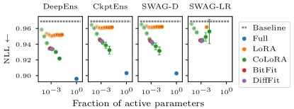
Figure 1: Negative log-likelihood for all combinations of inference and PEFT methods under consideration, evaluated on the NYU data set. Except SWAG-LR, all methods achieve improved NLL over the deterministic baseline. Error bars indicate 95% intervals across 5 replicate runs. Numbers in the dots indicate the rank parameter used.

We measure predictive performance by evaluating the negative log-likelihood (NLL) on an unseen test split for NYU and KITTI. We report the results in Figure 1 and Figure 4(a). We observe improvements when using Bayesian inference on either the full parameter space or just a PEFT subspace. Performing inference on the full parameter space achieves the best performance across all inference methods, except low-rank plus diagonal SWAG (SWAG-LR), where the evaluation failed due to numerical issues. For inference on the PEFT subspaces, we observe the most improvements using CoLoRA with a rank of at least 16, after which it begins to outperform BitFit and DiffFit, when using DeepEns, CkptEns, or SWAG-D. Most remarkably, CoLoRA seems to interpolate between the deterministic baseline and the full parameter space, if the rank parameter is increased. For LoRA, we observe improvement over the baseline already for rank 1. However, quite surprisingly, increasing the rank seems to yield only a small further improvement.

In terms of inference methods, we observe that DeepEns, although consisting only of 5 different parameter samples, yields better performance than all other methods, where prediction is performed using 100 parameter samples. Moreover, we observe little difference between SWAG-D and CkptEns. For SWAG-LR, we had numerical issues on the NYU data set, resulting in degraded performance for CoLoRA at ranks above 16, as well as missing evaluation for LoRA (except rank 16). For KITTI, we observe similar results for CkptEns and SWAG-D (c.f., Figure 4(a)).

4.2 Calibration

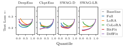
Figure 2: Test loss per quantile of most certain predictions evaluated on the NYU data set. Except DeepEns, all methods achieve improved test loss on more certain pixels, suggesting good calibration. Uncertainty was estimated using pixelwise standard deviation. For LoRA and CoLoRA, only the results for the rank with lowest test loss on the 5% quantile are depicted. The prediction using the publicly available checkpoint was used as a baseline. Shaded areas indicate 95% intervals across 5 replicate runs.

We further evaluated the calibration of the uncertainties obtained from Bayesian inference on PEFT subspaces by evaluating the test loss on quantiles of most certain pixels, as suggested in [4]. As an uncertainty metric, we consider the pixel-wise standard deviation. Results are depicted in Figure 2 and Figure 4(b). Note that for LoRA and CoLoRA, we only included the methods with smallest test loss on the 5% quantile of most certain pixels. Contrary to the previous section, we observe the worst performance for DeepEns, where the test loss decreases instead of increasing on the most certain pixels. However, similar to the results from the previous section, we observe the best performance using DeepEns on the full parameter space. For CkptEns and SWAG-D, inference on the full parameter space performs a bit worse than BitFit and DiffFit, especially on the most certain pixels. SWAG-LR overall achieves the smallest test loss on approximately 50% of the most certain pixels when using BitFit and DiffFit. Quite interestingly, we observe BitFit to be slightly better calibrated than DiffFit, although the latter uses more parameters. On NYU (c.f., Figure 2), CoLoRA is outperformed by the other methods when using SWAG, however on KITTI (c.f., Figure 4(b)), CoLoRA is often the only method achieving test loss smaller than the baseline.

Furthermore, we analyze the influence of the rank parameter on calibration by considering the test loss at the 25%, 50%, and 75% quantiles against the rank parameters. Results are depicted in Figure 3 and Figure 4(c). For both data sets, the results are fairly noisy and do not suggest a clear trend favoring higher ranks and thus, more parameters. Interestingly, rank $r=4$ seems to work particularly well for both data sets when using CkptEns.

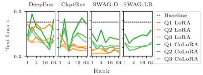
Figure 3: Test loss on 25%, 50%, and 75% quantiles for LoRA and CoLoRA against the rank parameter, evaluated on the NYU data set. No clear trend suggesting the usage of higher ranks can be identified. Shaded areas indicate 95% intervals across 5 replicate runs.

5 Conclusion

We demonstrated the applicability of PEFT subspaces for Bayesian deep learning on a modern Transformer-based computer vision architecture for monocular depth estimation. We show that simple methods like checkpoint ensembles and SWAG are capable of improving predictive performance and providing well-calibrated uncertainty estimates. Moreover, we propose a novel approach for constructing LoRA-like subspaces in convolutional layers, termed CoLoRA, and demonstrate that it performs competitively with the other PEFT methods. We hope that CoLoRA can also serve to make existing, convolution-based architectures uncertainty-aware in a parameter-efficient manner.

Appendix A Experiment Details

Fine-tuning is performed for 20 more epochs, starting from the checkpoints provided by Yang et al. [28]. During fine-tuning take 100 equidistant checkpoints. For both SWAG variants, we also draw 100 samples from the approximate posterior. For LoRA and CoLoRA, which admit a rank parameter, we test ranks 1, 2, 4, 8, 16, 32 and 64. For every combination of posterior approximation and PEFT method, we perform 5 replicate experiments using different seeds. For DeepEns, we use the last checkpoint from the five replicates to compile an ensemble. For all experiments, we use Adam [12] with a constant learning rate of 1e-7. The batch size for all methods is set to 4.

Appendix B Results on KITTI.

We provide figures for the analyses from Section 4 on the KITTI data set in Figure 4.

(a) Negative log-likelihood and mean test loss for all combinations of inference and PEFT methods under consideration, evaluated on the KITTI data set. Except SWAG-LR, all methods achieve improved NLL over the deterministic baseline. Error bars indicate 95% intervals across 5 replicate runs.

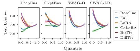
(b) Test loss per quantile of most certain predictions evaluated on the KITTI data set. Except DeepEns, all methods achieve improved test loss on more certain pixels, suggesting good calibration. Uncertainty was estimated either using pixelwise standard deviation. For LoRA and CoLoRA, only the methods with lowest test loss on the 5% quantile are depicted. The prediction using the publicly available checkpoint was used as a baseline. Shaded areas indicate 95% intervals across 5 replicate runs.

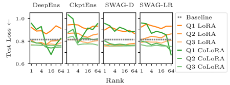
(c) Test loss on 25%, 50%, and 75% quantiles for LoRA and CoLoRA against the rank parameter, evaluated on the KITTI data set. No clear trend suggesting the usage of higher ranks can be identified. Shaded areas indicate 95% intervals across 5 replicate runs.

Figure 4: Evaluations on KITTI data set.

Appendix C Tucker Decomposition

For an $n$-tensor $A$ of size $h_{1}\times\cdots\times h_{n}$, the Tucker decomposition returns a core tensor $C\in\operatorname{\mathbb{R}}^{r_{1}\times\cdots\times r_{n}}$ and $n$ factor matrices $U^{(1)},\ldots,U^{(n)}\in\operatorname{\mathbb{R}}^{h_{i}\times r_{i}}$, where $r_{1},\ldots,r_{n}$ are the ranks along each of the $n$ tensor dimensions. From the Tucker decomposition, $A$ is recovered as

$$\begin{aligned} a_{i_{1},\ldots,i_{n}}=\sum_{j_{1}=1}^{r_{1}}\cdots\sum_{j_{n}=1}^{r_{n}}c_{j_{1},\ldots,j_{n}}\cdot u^{(1)}_{i_{1},j_{1}}\cdots u^{(n)}_{i_{n},j_{n}}.\end{aligned}$$ (8)

A low-rank approximation of $A$ can be computed by choosing the ranks $r_{1},\ldots,r_{n}$ of the decomposition to be less than the full ranks. Moreover, in the partial Tucker decomposition, we may choose to omit decomposition of certain tensor dimensions of the incoming $A$ tensor, in which case the core matrix $C$ simply takes full size $r_{i}=h_{i}$ along the respective tensor dimension $i$ and the corresponding factor matrix $U^{(i)}=I\in\operatorname{\mathbb{R}}^{h_{i}\times h_{i}}$ becomes an identity matrix. If the first $n$ tensor dimensions are chosen as low-rank, the corresponding decomposition is also commonly called Tucker-$n$ decomposition.

References

- [1] Marcella Astrid and Seung-Ik Lee. CP-decomposition with Tensor Power Method for Convolutional Neural Networks Compression, Jan. 2017. arXiv:1701.07148 [cs].
- [2] Tom Brown, Benjamin Mann, Nick Ryder, Melanie Subbiah, Jared D Kaplan, Prafulla Dhariwal, Arvind Neelakantan, Pranav Shyam, Girish Sastry, Amanda Askell, Sandhini Agarwal, Ariel Herbert-Voss, Gretchen Krueger, Tom Henighan, Rewon Child, Aditya Ramesh, Daniel Ziegler, Jeffrey Wu, Clemens Winter, Chris Hesse, Mark Chen, Eric Sigler, Mateusz Litwin, Scott Gray, Benjamin Chess, Jack Clark, Christopher Berner, Sam McCandlish, Alec Radford, Ilya Sutskever, and Dario Amodei. Language Models are Few-Shot Learners. In Advances in Neural Information Processing Systems, volume 33, pages 1877–1901. Curran Associates, Inc., 2020.
- [3] Hugh Chen, Scott Lundberg, and Su-In Lee. Checkpoint Ensembles: Ensemble Methods from a Single Training Process, Oct. 2017. arXiv:1710.03282 [cs].
- [4] Kamil Ciosek, Vincent Fortuin, Ryota Tomioka, Katja Hofmann, and Richard Turner. Conservative Uncertainty Estimation By Fitting Prior Networks. In International Conference on Learning Representations, Apr. 2020.
- [5] A Geiger, P Lenz, C Stiller, and R Urtasun. Vision meets robotics: The KITTI dataset. The International Journal of Robotics Research, 32(11):1231–1237, Sept. 2013. Publisher: SAGE Publications Ltd STM.
- [6] Andrew Gelman, Aki Vehtari, Daniel Simpson, Charles C. Margossian, Bob Carpenter, Yuling Yao, Lauren Kennedy, Jonah Gabry, Paul-Christian Bürkner, and Martin Modrák. Bayesian Workflow, Nov. 2020. arXiv:2011.01808 [stat].
- [7] Xavier Glorot and Yoshua Bengio. Understanding the difficulty of training deep feedforward neural networks. In Proceedings of the Thirteenth International Conference on Artificial Intelligence and Statistics, pages 249–256. JMLR Workshop and Conference Proceedings, Mar. 2010. ISSN: 1938-7228.
- [8] Frank L. Hitchcock. The Expression of a Tensor or a Polyadic as a Sum of Products. Journal of Mathematics and Physics, 6(1-4):164–189, 1927.
- [9] Edward J. Hu, Yelong Shen, Phillip Wallis, Zeyuan Allen-Zhu, Yuanzhi Li, Shean Wang, Lu Wang, and Weizhu Chen. LoRA: Low-Rank Adaptation of Large Language Models, Oct. 2021. arXiv:2106.09685 [cs].
- [10] Stefan Kesselheim, Andreas Herten, Kai Krajsek, Jan Ebert, Jenia Jitsev, Mehdi Cherti, Michael Langguth, Bing Gong, Scarlet Stadtler, Amirpasha Mozaffari, et al. Juwels booster–a supercomputer for large-scale ai research. In International Conference on High Performance Computing, pages 453–468. Springer, 2021.
- [11] Yong-Deok Kim, Eunhyeok Park, Sungjoo Yoo, Taelim Choi, Lu Yang, and Dongjun Shin. Compression of Deep Convolutional Neural Networks for Fast and Low Power Mobile Applications, Feb. 2016. arXiv:1511.06530 [cs].
- [12] Diederik P. Kingma and Jimmy Ba. Adam: A method for stochastic optimization. In Yoshua Bengio and Yann LeCun, editors, 3rd International Conference on Learning Representations, ICLR 2015, San Diego, CA, USA, May 7-9, 2015, Conference Track Proceedings, 2015.
- [13] Alexander Kirillov, Eric Mintun, Nikhila Ravi, Hanzi Mao, Chloe Rolland, Laura Gustafson, Tete Xiao, Spencer Whitehead, Alexander C. Berg, Wan-Yen Lo, Piotr Dollar, and Ross Girshick. Segment Anything. In Proceedings of the IEEE/CVF International Conference on Computer Vision, pages 4015–4026, 2023.
- [14] Wesley J Maddox, Pavel Izmailov, Timur Garipov, Dmitry P Vetrov, and Andrew Gordon Wilson. A Simple Baseline for Bayesian Uncertainty in Deep Learning. In Advances in Neural Information Processing Systems, volume 32. Curran Associates, Inc., 2019.
- [15] Prasanna Mayilvahanan, Thaddäus Wiedemer, Evgenia Rusak, Matthias Bethge, and Wieland Brendel. Does CLIP’s generalization performance mainly stem from high train-test similarity? In NeurIPS 2023 Workshop on Distribution Shifts: New Frontiers with Foundation Models, 2024.
- [16] Emre Onal, Klemens Flöge, Emma Caldwell, Arsen Sheverdin, and Vincent Fortuin. Gaussian Stochastic Weight Averaging for Bayesian Low-Rank Adaptation of Large Language Models, May 2024. arXiv:2405.03425 [cs].
- [17] Maxime Oquab, Timothée Darcet, Théo Moutakanni, Huy V. Vo, Marc Szafraniec, Vasil Khalidov, Pierre Fernandez, Daniel Haziza, Francisco Massa, Alaaeldin El-Nouby, Mido Assran, Nicolas Ballas, Wojciech Galuba, Russell Howes, Po-Yao Huang, Shang-Wen Li, Ishan Misra, Michael Rabbat, Vasu Sharma, Gabriel Synnaeve, Hu Xu, Herve Jegou, Julien Mairal, Patrick Labatut, Armand Joulin, and Piotr Bojanowski. DINOv2: Learning Robust Visual Features without Supervision. Transactions on Machine Learning Research, July 2023.
- [18] Theodore Papamarkou, Maria Skoularidou, Konstantina Palla, Laurence Aitchison, Julyan Arbel, David Dunson, Maurizio Filippone, Vincent Fortuin, Philipp Hennig, Jose Miguel Hernandez Lobato, Aliaksandr Hubin, Alexander Immer, Theofanis Karaletsos, Mohammad Emtiyaz Khan, Agustinus Kristiadi, Yingzhen Li, Stephan Mandt, Christopher Nemeth, Michael A. Osborne, Tim G. J. Rudner, David Rügamer, Yee Whye Teh, Max Welling, Andrew Gordon Wilson, and Ruqi Zhang. Position Paper: Bayesian Deep Learning in the Age of Large-Scale AI, Feb. 2024. arXiv:2402.00809 [cs, stat].
- [19] Alec Radford, Jong Wook Kim, Chris Hallacy, Aditya Ramesh, Gabriel Goh, Sandhini Agarwal, Girish Sastry, Amanda Askell, Pamela Mishkin, Jack Clark, Gretchen Krueger, and Ilya Sutskever. Learning Transferable Visual Models From Natural Language Supervision. In Proceedings of the 38th International Conference on Machine Learning, pages 8748–8763. PMLR, July 2021. ISSN: 2640-3498.
- [20] Rene Ranftl, Alexey Bochkovskiy, and Vladlen Koltun. Vision Transformers for Dense Prediction. In 2021 IEEE/CVF International Conference on Computer Vision (ICCV), pages 12159–12168, Montreal, QC, Canada, Oct. 2021. IEEE.
- [21] René Ranftl, Katrin Lasinger, David Hafner, Konrad Schindler, and Vladlen Koltun. Towards Robust Monocular Depth Estimation: Mixing Datasets for Zero-Shot Cross-Dataset Transfer. IEEE Transactions on Pattern Analysis and Machine Intelligence, 44(3):1623–1637, Mar. 2022. Conference Name: IEEE Transactions on Pattern Analysis and Machine Intelligence.
- [22] Nathan Silberman, Derek Hoiem, Pushmeet Kohli, and Rob Fergus. Indoor Segmentation and Support Inference from RGBD Images. In Andrew Fitzgibbon, Svetlana Lazebnik, Pietro Perona, Yoichi Sato, and Cordelia Schmid, editors, Computer Vision – ECCV 2012, pages 746–760, Berlin, Heidelberg, 2012. Springer.
- [23] Philipp Thörnig. Jureca: Data centric and booster modules implementing the modular supercomputing architecture at jülich supercomputing centre. Journal of large-scale research facilities JLSRF, 7:A182–A182, 2021.
- [24] Hugo Touvron, Thibaut Lavril, Gautier Izacard, Xavier Martinet, Marie-Anne Lachaux, Timothée Lacroix, Baptiste Rozière, Naman Goyal, Eric Hambro, Faisal Azhar, Aurelien Rodriguez, Armand Joulin, Edouard Grave, and Guillaume Lample. LLaMA: Open and Efficient Foundation Language Models, Feb. 2023. arXiv:2302.13971 [cs].
- [25] Ledyard R. Tucker. Some mathematical notes on three-mode factor analysis. Psychometrika, 31(3):279–311, Sept. 1966.
- [26] Enze Xie, Lewei Yao, Han Shi, Zhili Liu, Daquan Zhou, Zhaoqiang Liu, Jiawei Li, and Zhenguo Li. DiffFit: Unlocking Transferability of Large Diffusion Models via Simple Parameter-Efficient Fine-Tuning. In 2023 IEEE/CVF International Conference on Computer Vision (ICCV), pages 4207–4216, Paris, France, Oct. 2023. IEEE.
- [27] Adam X. Yang, Maxime Robeyns, Xi Wang, and Laurence Aitchison. Bayesian Low-rank Adaptation for Large Language Models, Feb. 2024. arXiv:2308.13111 [cs].
- [28] Lihe Yang, Bingyi Kang, Zilong Huang, Xiaogang Xu, Jiashi Feng, and Hengshuang Zhao. Depth Anything: Unleashing the Power of Large-Scale Unlabeled Data, Apr. 2024. arXiv:2401.10891 [cs].
- [29] Elad Ben Zaken, Shauli Ravfogel, and Yoav Goldberg. BitFit: Simple Parameter-efficient Fine-tuning for Transformer-based Masked Language-models, Sept. 2022. arXiv:2106.10199 [cs].