Long-distance device-independent quantum key distribution using single-photon entanglement
Abstract
Device-independent quantum key distribution (DIQKD) provides the strongest form of quantum security, as it allows two honest users to establish secure communication channels even when using fully uncharacterized quantum devices. The security proof of DIQKD is derived from the violation of a Bell inequality, mitigating side-channel attacks by asserting the presence of nonlocality. This enhanced security comes at the cost of a challenging implementation, especially over long distances, as losses make Bell tests difficult to conduct successfully. Here, we propose a photonic realization of DIQKD, utilizing a heralded preparation of a single-photon path entangled state between the honest users. Being based on single-photon interference effects, the obtained secret key rate scales with the square root of the quantum channel transmittance. This leads to positive key rates over distances of up to hundreds of kilometers, making the proposed setup a promising candidate for securing long-distance communication in quantum networks.
Exchanging private communication in a network is a central feature of the modern world. Classical protocols are based on computational security, as secrecy relies on computational assumptions. Quantum key distribution (QKD) [1, 2, 3, 4, 5] provides quantum physical security, an alternative solution in which two parties measure quantum states and obtain correlated classical bits, from which a secure key is constructed. No computational assumptions are needed, as these quantum correlations can be such that external adversaries cannot be correlated with the measurement outcomes, even when considering access to infinite computational power. The security of standard QKD protocols, however, relies on assumptions on the physics of the quantum devices used to distribute the key, in particular, it requires that these devices behave in the exact manner described by the protocol. In practice, verifying this assumption is challenging, as it demands accurate characterization of quantum states and measurements throughout the QKD protocol execution. In fact, by exploiting inaccurate quantum device calibrations, side-channel attacks have been successfully performed against QKD systems [6, 7, 8, 9]. To solve this critical problem, device-independent QKD (DIQKD) [10, 11, 12] protocols have been introduced: they use the violation of a Bell inequality to bound the information that adversaries may obtain on the distributed key, without requiring any modelling of the devices used in the protocol. DIQKD protocols therefore offer stronger security, as they are robust against any hacking attacks exploiting imperfections on the devices.
The implementation of DIQKD is challenging, as it requires the distribution of high-quality entangled states at long distances, as well as high-efficiency transmission channels and measurements. As photons in fibers are the natural carriers of quantum information, channel losses represent the main challenge for DIQKD: growing exponentially with distance, they become already at short distances too large for the honest users to be able to observe any Bell inequality violation [13]. To circumvent channel losses, a heralding scheme can be used, where entanglement is generated between the parties’ systems conditioned on the detection of photons at a central heralding station performing a joint measurement. Losses therefore reduce the key generation rate, but not its security. Heralding schemes have been used in recent proof-of-principle demonstrations of DIQKD [14, 15]. In these experiments, the honest users locally generate light-matter entanglement, so that the state at the local stations is encoded in material qubits. The photons are sent to the central station where the joint measurement heralds the preparation of an entangled state between the local material qubits. These can be measured with nearly perfect efficiency, which allows a large Bell inequality violation. Despite these successful demonstrations, the light-matter entanglement generation process required in this approach typically has low repetition rates, limiting its scalability over large distances. Purely photonic platforms are arguably the most suited for high-rate long-distance DIQKD applications [16, 17]. Several proposals for heralding photonic DIQKD exist, see for instance [18] or [19, 20]. However, these schemes require two-photon interference at the central heralding station, resulting in low repetition rates that make them impractical for long distances.
In this article, we propose a photonic DIQKD implementation that offers significant advantages with respect to the existing proposals. First of all, our scheme is based on single-photon interference effects. This results in much higher key rates, as they scale like the square root of the channel transmittance, as opposed to the previous schemes, which were based on two-photon interference and therefore had rates scaling like the channel transmittance. Single-photon interference is also at the heart of twin field QKD [21], a scheme that achieves the same scaling for the key rate, but needs to assume fully characterized preparation devices, unlike our device-independent scenario. This is possible because in our protocol single-photon interference is used to distribute a single-photon entangled state between the honest users, which is then measured to obtain the Bell violation required for device-independent QKD. Our second main ingredient in fact consists of a new scheme to observe Bell inequality violations from single-photon entangled states. This allows us to improve the robustness of the Bell test, in particular the detection efficiencies needed for secure key distribution.
We consider the scenario illustrated in Fig. 1a. Two honest users, Alice and Bob, possess a single-photon source that needs to be heralded, that is, such that Alice and Bob know when the single photon has been produced. The emitted photons are directed towards a beamsplitter with transmittance . This is a free parameter of the protocol that can be tuned to optimize the key rate, although in practice this transmittance needs to have a small value for reasons that will become clear below. So, it is convenient for what follows to consider that is small.
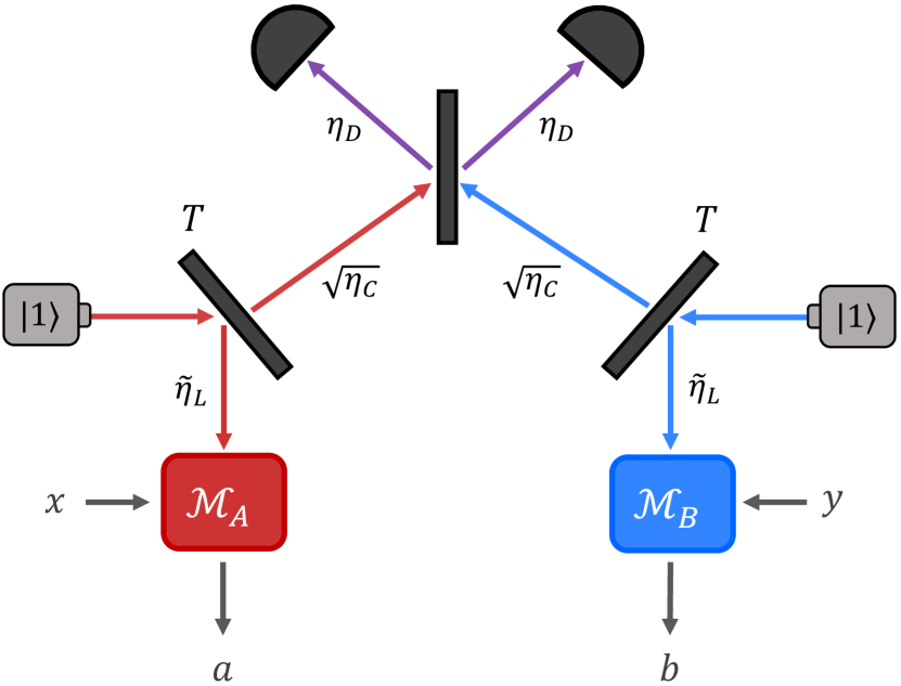
The transmitted modes are sent to a central station, named Charlie, through a lossy channel. For simplicity, we assume that Charlie is placed at half the distance between Alice and Bob. Let us denote by the efficiency of the channel directly connecting Alice and Bob. The dependence of on the distance is
| (1) |
where indicates the distance between Alice and Bob, and denotes the attenuation coefficient of the medium through which the photons travel. For optical fibers at telecommunication wavelengths, is typically . Since the distance between each honest user and Charlie is , the losses in the corresponding channels are the same and equal to . The reflected mode is directly sent to the measurement systems of either Alice or Bob. The bipartite state of Alice/Bob and Charlie, expressed in the photon-number basis, is given by
| (2) |
where is the state of a photon after the unbalanced beamsplitter.
At Charlie’s station, the two modes are combined into a balanced beamsplitter that erases the path information. The output modes are measured with photo-detectors of efficiency equal to . Charlie announces the measurement results, keeping those instances where only one of the two detectors clicks, while the others are discarded. When is small, a click on one of Charlie’s detectors heralds the state
| (3) |
between Alice and Bob at leading order in (see Supplementary Material B for more details). This is because is chosen small enough so that the probability that one photon has been transmitted in Alice or Bob’s locations and detected by Charlie is much larger than the probability that the two photons are sent to Charlie and one is detected. At first order in , a successful heralding happens with probability , with . The entangled state (3) is sent into the measurement devices and on Alice and Bob’s locations to establish the secret key. This process is not ideal and adds some additional losses encapsulated by an efficiency . We consider the protocol introduced in [11] based on the violation of the Clauser-Horne-Shimony-Holt (CHSH) inequality [23]. In this protocol, Alice (Bob) applies two (three) measurements, labeled by (), all with two possible outcomes, labeled by . We use and to denote the quantum observable measured by Alice and Bob. Rounds with and are referred to as key rounds and are used to construct the key. It is therefore required that these measurements give correlated results between Alice and Bob.
Rounds with and are referred to as test rounds, and use to compute the CHSH Bell expression
| (4) |
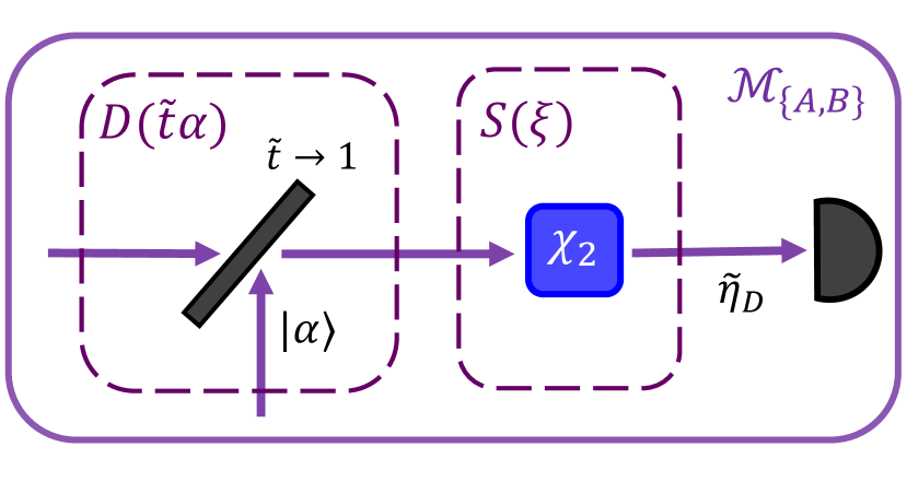
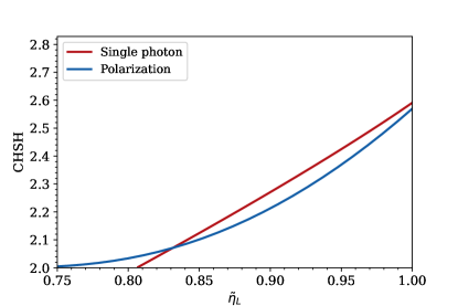
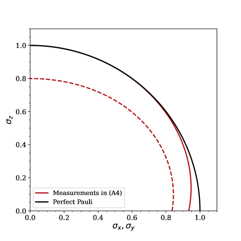
which is bounded by 2 for local models. From the CHSH value, it is possible to bound the maximum information that a quantum eavesdropper has on Alice’s outcomes for any of the CHSH settings. For example, for it is bound by the conditional entropy (see [11]). Measurements in the test round therefore need to be chosen to maximize the CHSH value observed by Alice and Bob. This requires projective measurements in bases involving superposition of the photonic qubit , which is not possible using only a single-photon detector. To solve this problem, we approximate these ideal measurements by means of Gaussian operations and photo-detectors, all routinely used in labs. In particular, we consider a displacement operator, followed by a nonlinear crystal and a single-photon detector with efficiency (see Fig. 1b). The displacement operation allows to project on noisy superposition of orthogonal photonic qubit state [24] while the non linear crystal increases the distinguishability between those states (see Supplementary Material A). When applied to the heralded state, the resulting measurements and allow getting CHSH violations close to the theoretical maximum and with significant noise robustness (see Fig. 2).
Once all the ingredients of the setup are defined, the expected key rates can be computed. To do so, we use the Devetak-Winter bound [25]
| (5) |
which provides a lower bound on the asymptotic key rate of the DIQKD protocol. While it is possible to compute directly from the statistics of the scenario previously described, cannot be directly assessed. Hence, we rely on the analytical lower bound introduced in [26]
| (6) | ||||
where represents the binary entropy of , stands for the CHSH score, and indicates the probability of Alice performing a bit-flip on her outcome. This noisy pre-processing step by Alice can indeed be used to optimize the lower bound on the key rate, as the maximum of (6) is in general obtained for a non-zero value of . For each value of the overall local efficiency , we evaluated Eq. (6) by expressing the CHSH score in terms of the parameterized measurements and depicted in Figure 1b and described in Supplementary Material A. For our protocol, we consider single-photon detectors with efficiency [27]. We find that the threshold local efficiency, including the detector and losses, required to generate a key is .
For the experimental realization of DIQKD, we explore the impact of a limited number of protocol rounds on the achievable key rate. This constraint, together with the heralding probability scaling with , inherently reduce the length of the secure key. Consequently, we provide a security proof against general attacks for our protocol, considering a finite number of runs. For this purpose, we use the entropy accumulation theorem (EAT) [28] which bound the uncertainty of an eavesdropper after rounds. This is achieved by calculating the von Neumann entropy for each round and applying a correction factor based on the specific protocol. We apply the EAT to our protocol following the methodology outlined in [14]. A comprehensive description of the functions employed to compute the length of the secure key for a specified number of rounds is provided in Supplementary Material C. Thus, the key rate is computed as . As , the key rate converges to its asymptotic value (6). Finally, by considering the source’s generation rate and the heralding probability , the key rate can be expressed as
| (7) |
There are at the moment two main approaches to generate single photons in a heralded way: using spontaneous parametric down-conversion (SPDC) or quantum dots. The first offers high distinguishability with frequency generation of the order of hundreds of MHz [29], while the latter provides brighter single-photon emission, although with a frequency generation of the order of a few MHz [30]. In this work, we set , corresponding to state-of-the-art SPDC sources.
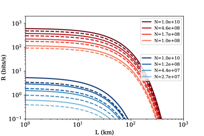
Previous proposals for photonic heralded DIQKD schemes encode the key in a degree of freedom that requires physical support, e.g., polarization. This demands two-photon interference at the central station [19, 14, 15]. In these cases, the heralding probability scales as
| (8) |
that is, proportional to the channel transmittance instead of its square root, as in our scheme. This results in much smaller key rates. To illustrate the superior performance of our proposal, we compare in Fig. 3 the key rate as a function of the distance for our scheme (red) and for the heralded DIQKD scheme of [20] based on polarization (blue). Our analysis shows a significantly improved performance, enabling secure quantum communication over much larger distances.
This work presents a proposal for photonic DIQKD that significantly improves over previous solutions, as it combines the best implementation aspects of twin-field QKD with the security guarantees of DIQKD. In fact, its key rate scales as the square root of the transmittance between the honest users, as in twin-field, while not requiring any characterization of the devices, as in DIQKD. Moreover, our proposal also presents relevant improvements on the efficiencies and losses needed in the local labs by Alice and Bob. The required values remain challenging, of the order of , but within reach for current or near-term technologies. Putting all these considerations together, our results provide a robust solution for achieving photonic secure key distribution over long distances through DIQKD.
Acknowledgements
This work is supported by the Government of Spain (Severo Ochoa CEX2019-000910-S, FUNQIP, NextGenerationEU PRTR-C17.I1), EU projects QSNP, Quantera Veriqtas, Fundació Cellex, Fundació Mir-Puig, Generalitat de Catalunya (CERCA program), the ERC AdG CERQUTE and the AXA Chair in Quantum Information Science. A.S. acknowledges support from the “Agencia Estatal de Investigación” (Ref. PRE2022-101475). M.N. acknowledges funding from the European Union’s Horizon Europe research and innovation programme under the Marie Skłodowska-Curie Grant Agreement No. 101081441. X.V. acknowledges funding by the European Union’s Horizon Europe research and innovation program under the project “Quantum Security Networks Partnership” (QSNP, Grant Agreement No. 101114043). X.V and E.O acknowledge funding by the French national quantum initiative managed by Agence Nationale de la Recherche in the framework of France 2030 with the reference ANR-22-PETQ-0009.
Code availability
Code is available via Github at ref. [31]. Additional inquiries about this code should be directed to A.S (anna.steffinlongo@icfo.eu).
References
- Bennett and Brassard [1984] C. H. Bennett and G. Brassard, Proceedings of IEEE International Conference on Computers, Systems, and Signal Processing , 175 (1984).
- Ekert [1991] A. K. Ekert, Physical Review Letters 67, 661 (1991).
- Gisin et al. [2002] N. Gisin, G. Ribordy, W. Tittel, and H. Zbinden, Reviews of Modern Physics 74, 145 (2002).
- Lo et al. [2014] H.-K. Lo, M. Curty, and K. Tamaki, Nature Photonics 8, 595 (2014).
- Scarani et al. [2009] V. Scarani, H. Bechmann-Pasquinucci, N. J. Cerf, M. Dušek, N. Lütkenhaus, and M. Peev, Reviews of Modern Physics 81, 1301 (2009).
- Gerhardt et al. [2011] I. Gerhardt, Q. Liu, A. Lamas-Linares, J. Skaar, C. Kurtsiefer, and V. Makarov, Nature Communications 2, 1348 (2011).
- Lydersen et al. [2010] L. Lydersen, C. Wiechers, C. Wittmann, D. Elser, J. Skaar, and V. Makarov, Nature Photonics 4, 686 (2010).
- Zhao et al. [2008] Y. Zhao, C.-H. F. Fung, B. Qi, C. Chen, and H.-K. Lo, Physical Review A 78, 042333 (2008).
- Weier et al. [2011] H. Weier, H. Krauss, M. Rau, M. Fürst, S. Nauerth, and H. Weinfurter, New Journal of Physics 13, 073024 (2011).
- Mayers and Yao [2004] D. Mayers and A. Yao, Quantum Information and Computation 4, 273 (2004).
- Acín et al. [2007] A. Acín, N. Brunner, N. Gisin, S. Massar, S. Pironio, and V. Scarani, Physical Review Letters 98, 230501 (2007).
- Vazirani and Vidick [2014] U. Vazirani and T. Vidick, Physical Review Letters 113, 140501 (2014).
- Acín et al. [2016] A. Acín, D. Cavalcanti, E. Passaro, S. Pironio, and P. Skrzypczyk, Phys. Rev. A 93, 012319 (2016).
- Nadlinger et al. [2022] D. P. Nadlinger, P. Drmota, B. C. Nichol, G. Araneda, D. Main, R. Srinivas, D. M. Lucas, C. J. Ballance, K. Ivanov, E. Y.-Z. Tan, P. Sekatski, R. L. Urbanke, R. Renner, N. Sangouard, and J.-D. Bancal, Nature 607, 682–686 (2022).
- Zhang et al. [2022] W. Zhang, T. van Leent, K. Redeker, R. Garthoff, R. Schwonnek, F. Fertig, S. Eppelt, W. Rosenfeld, V. Scarani, C. C.-W. Lim, and H. Weinfurter, Nature 607, 687–691 (2022).
- Zapatero et al. [2023] V. Zapatero, T. van Leent, R. Arnon-Friedman, W.-Z. Liu, Q. Zhang, H. Weinfurter, and M. Curty, npj Quantum Information 9, 10.1038/s41534-023-00684-x (2023).
- Valcarce [2023] X. Valcarce, Device-independent certification: quantum resources and quantum key distribution, Theses, Université Paris-Saclay (2023).
- Gisin et al. [2010] N. Gisin, S. Pironio, and N. Sangouard, Phys. Rev. Lett. 105, 070501 (2010).
- Kołodyński et al. [2020] J. Kołodyński, A. Máttar, P. Skrzypczyk, E. Woodhead, D. Cavalcanti, K. Banaszek, and A. Acín, Quantum 4, 260 (2020).
- González-Ruiz et al. [2024] E. M. González-Ruiz, J. Rivera-Dean, M. F. B. Cenni, A. S. Sørensen, A. Acín, and E. Oudot, Opt. Express 32, 13181 (2024).
- Lucamarini et al. [2018] M. Lucamarini, Z. L. Yuan, J. F. Dynes, and A. J. Shields, Nature 557, 400 (2018).
- Paris [1996] M. G. Paris, Physics Letters A 217, 78 (1996).
- Clauser et al. [1969] J. F. Clauser, M. A. Horne, A. Shimony, and R. A. Holt, Phys. Rev. Lett. 23, 880 (1969).
- Banaszek and Wódkiewicz [1999] K. Banaszek and K. Wódkiewicz, Physical Review Letters 82, 2009–2013 (1999).
- Devetak and Winter [2005] I. Devetak and A. Winter, Proceedings of the Royal Society A: Mathematical, Physical and engineering sciences 461, 207 (2005).
- Ho et al. [2020] M. Ho, P. Sekatski, E. Y.-Z. Tan, R. Renner, J.-D. Bancal, and N. Sangouard, Phys. Rev. Lett. 124, 230502 (2020).
- Reddy et al. [2019] D. V. Reddy, R. R. Nerem, A. E. Lita, S. W. Nam, R. P. Mirin, and V. B. Verma, Conference on Lasers and Electro-Optics, Conference on Lasers and Electro-Optics , FF1A.3 (2019).
- Dupuis et al. [2020] F. Dupuis, O. Fawzi, and R. Renner, Communications in Mathematical Physics 379, 867–913 (2020).
- Tomm et al. [2021] N. Tomm, A. Javadi, N. O. Antoniadis, D. Najer, M. C. Löbl, A. R. Korsch, R. Schott, S. R. Valentin, A. D. Wieck, A. Ludwig, and R. J. Warburton, Nature Nanotechnology 16, 399–403 (2021).
- Liu et al. [2022] W.-Z. Liu, Y.-Z. Zhang, Y.-Z. Zhen, M.-H. Li, Y. Liu, J. Fan, F. Xu, Q. Zhang, and J.-W. Pan, Phys. Rev. Lett. 129, 050502 (2022).
- Steffinlongo [2024] A. Steffinlongo, https://github.com/annasteffinlongo/diqkd-with-single-photons (2024).
- Tan et al. [2022] E. Y.-Z. Tan, P. Sekatski, J.-D. Bancal, R. Schwonnek, R. Renner, N. Sangouard, and C. C.-W. Lim, Quantum 6, 880 (2022).
Supplementary Material
Appendix A Squezed Displaced Measurements
In this section, we present the novel measurements performed by Alice and Bob to observe a Bell inequality violation. In particular, we focus on a 2-outcome POVM comprising a displacement and a squeezing operator, followed by a single-photon detector. The two possible outcomes we consider are , when the detector does not click, and when it clicks. The corresponding POVM elements read
| (9) | ||||
| (10) |
Here and correspond to the displacement and squeezing operator, respectively. The arguments of these operators are complex numbers, such as and . Note that to account for imperfect detectors, we can replace the vacuum projector in (9) by the state . Since we are interested in using such measurement on the heralded state in Eq. (3), we focus on its projection on the qubit space spanned by and . An arbitrary 2-outcome qubit POVM can be written
| (11) |
where and quantify the projective and the random part of the measurement respectively (random in the sense that it gives the same value for all the incoming states). The two vectors are orthogonal and quantifies the ability of the POVM to distinguish between these two orthogonal states. To identify the projective part of the POVM when projected into the subspace, we first write a displaced squeezed vacuum in the Fock basis: Then, the matrix elements of the POVM (9) are
| (12) |
where we explicitly write
| (13) |
being the Hermite polynomials of order . Following Eq. (11), the projective part of the POVM in the direction is given by
| (14) |
where . Inserting the POVM in Eq. (14) we get
| (15) |
This quantifies how well we can mimic a Pauli measurement in the direction defined in the photonic qubit space using the POVM described in Figure 1b. For each we then optimize according to
| (16) |
In Fig. 4 we present the projection along all the possible directions in the positive and planes, where are the Pauli matrices.
Appendix B Heralded State
In this section, we derived the heralded state as a function of the transmittance . Given that the heralding probability is directly proportional to the key rate (7), selecting an optimal value for becomes crucial. This value should be sufficiently small to herald the state described in Eq. (3) while ensuring high key rates. We begin by considering the state of the photons emitted by an ideal single-photon source, which can be expressed as . According to the setup illustrated in Fig. 1a, these photons are directed towards an unbalanced beamsplitter with transmittance . This optical device undergoes the following transformation
| (17) |
Applying this transformation to the initial state , we can construct the density matrix after the unbalanced beamsplitter. Since the coefficient is small, we keep the terms proportional to and neglect higher-order terms. The resulting density matrix is given by
| (18) |
In this expression, the first () and second () path modes correspond to the reflected photons from Alice’s and Bob’s unbalanced beamsplitters, respectively. The third () and fourth () path modes represent the transmitted photons. Before these photons in the modes reach the central station, they pass through a lossy channel, which we model as a beamsplitter where the reflected photons are sent to the environment. Note that Charlie’s balanced beamsplitter commutes with the beamsplitter used to model the detector efficiency . As a result, we can combine the effects of channel losses and detector imperfections into a single efficiency parameter, , where represents the efficiency of the channel linking Alice and Bob to Charlie. Thus, when we have an exclusively one-photon contribution (e.g., terms proportional to ) the channel transforms as follows
| (19) |
where the vacuum contribution appears only in pure density matrices. For terms proportional to , the channel behaves as
| (20) | |||
| (21) |
and similarly for the two other terms. In the particular case of the state the channel acts as
| (22) |
Applying these transformations to the state (18) we can construct the density matrix that describes the state reaching the central station. At this point, Charlie performs the following projective measurement
| (23) |
with BS being the unitary matrix of a beamsplitter. Hence, we obtain the heralded state
| (24) |
with probability , under the assumption . It is important to highlight that by taking the unnormalized heralded state and approximating , we can recover the entangled state (8). Once the state in Eq. (24) is heralded, it passes through a channel with efficiency . Consequently, the state measured by Alice and Bob becomes
| (25) |
Considering that Alice and Bob posses detectors with efficiency , their POVM element is given by
| (26) |
with .
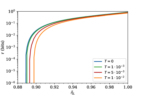
Finally, to determine an optimal value for the transmittance , we compare the asymptotic key rate from Eq.(6) when using the state in (25) and the measurement in (26) for different values of , as shown in Fig. 5. We conclude that offers a good balance, providing a robust efficiency threshold without significantly compromising the key rate.
Appendix C Finite-size analysis
In this section, we present the finite-size analysis we performed in order to take into account the limited number of protocols round on the key rate. We start by giving a definition of the soundness parameter and the completeness parameter [32]. The soundness parameter, , provides an upper bound on the distance between the state used for the protocol and the state where the honest parties have an identical key. This key should be completely independent of any side information possessed by an eavesdropper. In other words, measures the protocol’s resistance against attacks by an eavesdropper, ensuring that the final key shared by the honest parties remains close to perfect despite potential eavesdropping attempts. The completeness parameter, , is an upper bound on the probability of aborting the protocol when it is performed with honest devices. This parameter ensures that the protocol does not excessively terminate or abort when executed under normal, honest conditions. It helps quantifying the reliability and efficiency of the protocol when run with properly functioning devices.
In the following we define the functions that have been used for computing the key rate for finite-size statistics. We start by writing the CHSH-based entropy bound [26]
| (27) |
where is the bit-flip probability of the noisy preprocessing, , , with and , and represents the binary entropy. Then we can express the family of linear lower bounds on the entropy
| (28) |
from which we obtain
| (29) |
where are three delta distributions over , with indicating a key-round. If we introduce a probability distribution , we can define the following family of functions
| (30) |
with variance equal to
| (31) |
To compute the key rate, we also need the following functions
| (32) | ||||
| (33) |
We will employ the upper bound for , as its precise value can render numerical computations unstable. By considering the probability distribution , we can write
| (34) | ||||
| (35) |
Observe that
| (36) | ||||
| (37) |
We will also need to define
| (38) |
where is the principal branch of the Lambert function and . Finally, we introduce the parameters:
| (39) | ||||
Specifying the smoothing parameters such that
| (40) |
Utilizing the parameters and functions delineated so far, it can be shown (see [14]) that our protocol generates a ()+4)-sound key, with a length of
| (41) |
with
| (42) | ||||
Given that the values of have been set to , and is determined through the use of the VHASH algorithm, the protocol is proved to be sound. All the rest of the parameters, have been optimized to maximize . The value of the threshold CHSH winning probability and the length of the error correction syndrome were chosen according to those suggested in [14]. Specifically, we employed
| (43) | ||||
| (44) |
with , , , and representing the CHSH-score. This selection ensures that the completeness of the protocol is . As for the error correction syndrome we used
| (45) |
The CHSH-score and have been computed using the optimal measurements described in the Supplementary Material A for a fixed overall local efficiency . For computing the key rate we have imposed our protocol to be -complete and -sound.