The diverse star formation histories of early massive, quenched galaxies in modern galaxy formation simulations

Abstract

We present a comprehensive study of the star formation histories of massive-quenched galaxies at $z=3$ in $3$ semi-analytic models (Shark, GAEA, Galform) and $3$ cosmological hydrodynamical simulations (Eagle, Illustris-TNG, Simba). We study the predicted number density and stellar mass function of massive-quenched galaxies, their formation and quenching timescales and star-formation properties of their progenitors. Predictions are disparate in all these diagnostics, for instance: (i) some simulations reproduce the observed number density of very massive-quenched galaxies ($>10^{11}\,\rm M_{\odot}$) but underpredict the high density of intermediate-mass ones, while others fit well the lower masses but underpredict the higher ones; (ii) In most simulations, except for GAEA and eagle, most massive-quenched galaxies had starburst periods, with the most intense ones happening at $4<z<5$; however, only in Shark and Illustris-TNG we do find a large number of progenitors with star formation rates $>300\rm\,M_{\odot}\,yr^{-1}$; (iii) quenching timescales are in the range $\approx 20-150$ Myr depending on the simulation; among other differences. These disparate predictions can be tied to the adopted Active Galactic Nuclei (AGN) feedback model. For instance, the explicit black-hole (BH) mass dependence to trigger the “radio mode” in Illustris-TNG and Simba makes it difficult to produce quenched galaxies with intermediate stellar masses, also leading to higher baryon collapse efficiencies ($\approx 15-30$%); while the strong bolometric luminosity dependence of the AGN outflow rate in GAEA leads to BHs of modest mass quenching galaxies. Current observations are unable to distinguish between these different predictions due to the small sample sizes. However, these predictions are testable with current facilities and upcoming observations, allowing a “true physics experiment” to be carried out.

1 Introduction

Over the previous years, significant effort has been placed in to studying the number density of passive galaxies across cosmic time (e.g.Straatman et al. 2014; Schreiber et al. 2015, 2018; Merlin et al. 2019; Valentino et al. 2020; Shahidi et al. 2020; Carnall et al. 2020; Gould et al. 2023; Weaver et al. 2023). This field has seen an explosion of results thanks to the James Webb Space Telescope (JWST), which consistently reports high number densities of massive ($\gtrsim 10^{10}\,\rm M_{\odot})$, passive ($\rm sSFR\lesssim 10^{-10}\,yr^{-1}$) galaxies at redshifts $z>2$, even higher than the values claimed pre-JWST (Carnall et al., 2023a; Valentino et al., 2023; Nanayakkara et al., 2024; Long et al., 2023; Alberts et al., 2023). These observations have moved beyond reporting “candidates” for massive-quenched galaxies based on colours, with many now being spectroscopically confirmed (Carnall et al., 2023b, 2024; Nanayakkara et al., 2024; de Graaff et al., 2024; Weibel et al., 2024), with the highest redshift one being at $z\approx 7$ (Weibel et al., 2024). These studies are posing significant constraints on modern cosmological galaxy formation simulations, which for the most part seem to have difficulties in reproducing such high number densities (e.g. Valentino et al. 2023; Hartley et al. 2023; De Lucia et al. 2024; Lagos et al. 2024; Weller et al. 2024; Vani et al. 2024; de Graaff et al. 2024). There are exceptions though. For example, Remus & Kimmig (2023) show that in their simulation, the number of massive-quenched galaxies at $z\approx 3-5$ agrees reasonably well with observations within the uncertainties.

Beyond constraining the number density of massive, passive galaxies, the JWST has been used to get exquisite spectra of these galaxies, not only confirming their high redshifts ($z\gtrsim 3$), but also allowing intrinsic properties of galaxies to be inferred (e.g. Glazebrook et al. 2024; de Graaff et al. 2024; Carnall et al. 2023b, 2024; Nanayakkara et al. 2024). These galaxies tend to have large stellar masses ($\gtrsim 10^{10.3}\,\rm M_{\odot}$), and star formation histories (SFHs) indicative of relatively short-duration starbursts (few $\sim 100$ Myr). These observations are therefore offering a unique opportunity to piece together the picture of massive galaxy formation from the early to the local Universe.

In the local Universe, a consistent picture has emerged over the previous 20 years, in which some form of feedback (usually related to Active Galactic Nuclei; AGN) is responsible for quenching star formation in massive galaxies. This form of feedback is invoked by galaxy formation models and simulations to reproduce a plethora of phenomena observed in local massive galaxies, such as “downsizing”, the break in the stellar mass function, the optical colour-magnitude bimodality, among others (see e.g. Benson et al. 2003; Springel 2005; Croton et al. 2006; Bower et al. 2006; Lagos et al. 2008; Somerville et al. 2008; Sijacki et al. 2007; Cattaneo et al. 2008 to mention a few of the early studies on the topic). AGN feedback is thus generally used to reproduce the properties of massive galaxies locally and in fact the free-parameters of AGN feedback models are usually tuned for this exact purpose (e.g. Schaye et al. 2015; Crain et al. 2015; Croton et al. 2016; Weinberger et al. 2018; Davé et al. 2019; Kugel et al. 2023; Lagos et al. 2024; De Lucia et al. 2024). The process of tuning the free-parameters involved in the feedback models included in galaxy formation simulations has led to an overall agreement of broad statistics among simulations, such as the local Universe galaxy stellar mass function and the SFR-stellar mass relations (Somerville et al., 2015). Thus, testing the simulations in regimes that are far from those used for the tuning process is essential to understand how well current feedback models are doing in reproducing the diversity of galaxy properties observed across a wide range of cosmic epochs.

Although effectively all cosmological galaxy formation simulations invoke some form of AGN feedback to reproduce the properties of massive galaxies locally, in detail, the exact model employed can vary significantly between codes. For example, some models and simulations invoke only a single mode of AGN feedback (Schaye et al., 2015; Henriques et al., 2015; Lacey et al., 2016), while others invoke two modes (Weinberger et al., 2018; Davé et al., 2019; Lagos et al., 2024; De Lucia et al., 2024). Although these models do produce similar properties for massive galaxies in the local universe, by construction, they do it for very different reasons (see for example the differences in the halo gas reservoirs and gas in/out flow rates in the Eagle, Simba and Illustris-TNG simulations; Wright et al. 2024). The new wave of observations of massive-quenched galaxies at high redshift coming from the JWST offer a unique opportunity to stress-test galaxy formation models in a new territory for which parameters have not been tuned. Equally important is to explore whether the different AGN feedback models leave clear imprints on the properties of massive galaxies in the early universe that can now be inferred from the exquisite observations the JWST is providing.

In this paper we set up for this task by taking $6$ modern cosmological galaxy formation simulations ($3$ semi-analytic models, and $3$ cosmological hydrodynamical simulations) and analysing the high-z massive-quenched galaxies they predict to answer the following questions: (i) how well can modern galaxy formation simulations reproduce the number density and mass distributions of early massive-quenched galaxies? (ii) what is the diversity of SFHs predicted for early massive-quenched galaxies in modern simulations? (iii) if the differences are large, can we trace them back to the different ways in which feedback is modelled in the simulations?

This paper is organised as follows. § 2 describes the suite of galaxy formation simulations used in this work, and presents the samples and definitions employed in this paper. § 3 studies the number densities and stellar mass function of massive-quenched galaxies in the $6$ simulations analysed here and compares with observations. § 4 studies the SFHs of massive-quenched galaxies, focusing first on the rise of star formation, and then on how quenching happens and its relation to AGN feedback. In this section we also compare with observations where possible. § 5 presents our main conclusions. Appendix A presents an analysis of a control sample of massive, star-forming galaxies and how they sample the galaxy main sequence evolution; Appendix B shows the evolution of the number density of massive-quenched galaxies in the Magneticum simulation and compare with the other $6$ simulations used throughout this work. Appendix C evaluates the impact of the different time cadence of the simulations used here on the maximum SFR of galaxies. Appendix D presents the fits to the SFHs of galaxies in the simulations, which we use to quantify the frequency of starburst episodes.

2 The suite of galaxy formation simulations

In this section we briefly introduce the simulations used in this work. § 2.1 and § 2.2 describe the semi-analytic models and hydrodynamical simulations, respectively.

2.1 Semi-analytic models of galaxy formation

Semi-analytic models (SAMs) solve for the formation and evolution of galaxies using dark matter (DM) halo populations and merger trees built from DM-only $N$-body simulations. In the three models explored here, the following physical processes are modelled (i) the collapse and merging of DM halos; (ii) the accretion of gas onto halos; (iii) the shock heating and radiative cooling of gas inside DM halos, leading to the formation of galactic disks; (iv) star formation in galaxy disks; (v) stellar feedback from the evolving stellar populations; (vi) chemical enrichment of stars and gas; (vii) the growth via gas accretion and merging of black holes (BHs); (viii) heating by Active Galactic Nuclei (AGN); (ix) photoionisation of the intergalactic medium; (x) galaxy mergers which can trigger starbursts (starbursts) and the formation and/or growth of spheroids; (xi) effects of disk instabilities which in some models can trigger starbursts. In SAMs, the timescale in which galaxy mergers happen needs to be prescribed, and generally happens after the satellite subhalo that hosts a satellite galaxy ceases to be tracked due to its low number of DM particles.

The SAMs studied here differ in the way the different processes above are modelled. For the purpose of this paper, the key processes we are interested in are AGN feedback and the physical processes triggering starbursts, and hence we especially focus on describing the way these are modelled. Note that SAMs are sensitive to the number of snapshots produced with the $N$-body simulation (in a way that hydrodynamical simulations are not), and the disparate number of snapshots of the adopted simulations in the SAMs below will impact how finely we can sample the SFHs of galaxies.

2.1.1 Shark

Shark, (Lagos et al., 2018, 2024) is a publicly available code hosted on GitHub. We use the version of the code presented in Lagos et al. (2024), which was shown to produce massive galaxies whose properties agreed better with observations across a wide redshift range.

One of the novelties of Shark v2.0 presented in Lagos et al. (2024) is the AGN feedback model, which consists of two modes: a jet and a wind mode. The jet mode depends on the jet power produced by the AGN, $Q_{\rm jet}$, which in itself depends on the BH spin, accretion rate and mass (see Equation (31) in Lagos et al. 2024). For galaxies with an AGN, the cooling luminosity of the hot gas in the halo is offset by $Q_{\rm jet}$ (modulated by an efficiency parameter $\kappa_{\rm jet}$), which can completely shut off the cooling flow for sufficiently strong jets. The jet mode only acts on halos that have already formed a hot halo, following the model of Correa et al. (2018). The wind mode on the other side consists of a radiation pressure-driven outflow whose velocity depends on the dust opacity, gas content of the bulge and AGN bolometric luminosity (following the model of Ishibashi & Fabian 2015 - see Equation (36)). If the internal energy of the outflow exceeds the binding energy of the halo, then the outflow (or part of it) is allowed to escape the halo. This wind mode can only happen during starburst episodes, which in Shark can be triggered by galaxy mergers or disk instabilities. In the latter a stability parameter is computed with the properties of the galaxy disk, and if this is below a given threshold, then the disk of that galaxy is assumed to be fully destroyed, with all the gas and stellar content being moved to the bulge. The newly acquired gas of the bulge then is the fuel for the triggered starburst.

The free parameters of Shark were calibrated using an automatic optimiser that fits the $z<0.1$ stellar mass function (SMF). Although not used in the calibration, other results of the model were visually inspected to ensure their agreement with observations was not seriously compromised by the $z<0.1$ SMF only. Those included $z\approx 0$ gas scaling relations, the mass-metallicity relation and the $z<2$ cosmic specific star formation rate density (CSFRD).

Here we use a version of Shark running over the P-Millennium $N$-body simulation (P-MILL hereafter). P-MILL was introduced in Baugh et al. (2019) and the cosmological parameters correspond to a total matter, baryon and $\Lambda$ densities of $\Omega_{\rm m}=0.307$, $\Omega_{\rm b}=0.04825$ and $\Omega_{\Lambda}=0.693$, respectively, with a Hubble parameter of $H_{\rm 0}=h\,100\,\rm Mpc\,km\,s^{-1}$ with $h=0.6777$, scalar spectral index of $n_{\rm s}=0.9611$ and a power spectrum normalisation of $\sigma_{\rm 8}=0.8288$. P-MILL’s volume and particle mass are $(542.16\,\rm cMpc/h)^{3}$ (where cMpc refers to comoving megaparsec) and $1.06\times 10^{8}\,\rm M_{\odot}/h$, respectively. P-Mill has $271$ snapshots. Merger trees and halo catalogues for P-MILL were constructed using SUBFIND (Springel et al., 2001) and merger trees were built using D-halos (Jiang et al., 2014). Halos with $\geq 20$ particles are included in the catalogues, giving a minimum halo mass of $2.12\times 10^{9}\,\rm M_{\odot}/h$.

2.1.2 GAEA

GAlaxy Evolution and Assembly (GAEA) was introduced in De Lucia et al. (2014) and Hirschmann et al. (2016). Here, we use the latest GAEA version, introduced in De Lucia et al. (2024), which combined a new treatment of AGN feedback with an updated model of environmental processes affecting satellite galaxies. A key aspect highlighted in De Lucia et al. (2024) is that the new version of GAEA is able to reproduce the observed number densities of massive-quenched galaxies up to $z\approx 4$ (including some of the JWST ones).

The AGN feedback model of GAEA was first introduced in Fontanot et al. (2020), and consists of (i) a model for the inflow of cold gas towards the central BH driven by star formation in the central regions of galaxies; (ii) a BH accretion rate that is determined by the viscous accretion timescale; and (iii) an empirical scaling relation between the mass loading of quasar winds and the AGN bolometric luminosity. Note that the quasar outflow rate does not depend on the available interstellar medium reservoir, but only on the AGN bolometric luminosity. The treatment of disk instabilities in GAEA is markedly different from that in Shark and Galform. This is described in De Lucia et al. (2011) and in short the model computes the same instability parameter described in § 2.1.1 and if a disk is unstable, enough stellar mass is transferred from the disk to the bulge as to restore stability. Hence, there is no associated starburst with disk instabilities, but they can still contribute to the mass growth of bulges. Galaxy mergers are therefore the only route to produce starbursts in GAEA.

The free parameters in GAEA were tuned to reproduce the $z=0-3$ SMF, the atomic and molecular hydrogen mass functions in the local Universe, and the evolution of the AGN luminosity function up to $z=4$.

The version of GAEA used here was run over merger trees from the Millennium Simulation (Springel et al., 2005) (hereafter MILL), which adopts the following cosmological parameters, $\Omega_{\rm m}=0.25$, $\Omega_{\rm b}=0.045$, $\Omega_{\Lambda}=0.75$, $h=0.73$, $n_{\rm s}=1$, and $\sigma_{8}=0.8$. MILL has a volume of $(500\,\rm cMpc/h)^{3}$, a particle mass of $8.625\times 10^{8}\,\rm M_{\odot}/h$, and $64$ snapshots. Merger trees and halo catalogues for MILL were constructed using Sub-LINK and SUBFIND (Springel et al., 2001). Halos with $\geq 20$ particles are included in the catalogues, giving a minimum halo mass of $1.73\times 10^{10}\,\rm M_{\odot}/h$.

2.1.3 Galform

We use the Galform version introduced in Lacey et al. (2016), which combined several flavours of previous Galform model versions that focused on a variety of issues, such as reproducing the properties of massive galaxies and high-redshift star-forming galaxies.

The AGN feedback model adopted in Galform was introduced by Bower et al. (2006) and is assumed to be effective only in halos undergoing quasi-hydrostatic cooling. In this situation, mechanical energy input by the AGN is expected to stabilise the flow and regulate the rate at which the gas cools. Whether or not a halo is undergoing quasi-hydrostatic cooling depends on the cooling and free-fall times: the halo is in this regime if $t_{\rm cool}(r_{\rm cool})>\alpha^{-1}_{\rm cool}\,t_{\rm ff}(r_{\rm cool})$, where $t_{\rm ff}$ is the free fall time at $r_{\rm cool}$, and $\alpha_{\rm cool}\sim 1$ is an adjustable parameter close to unity. AGNs are assumed to be able to quench gas cooling only if the available AGN power is comparable to the cooling luminosity, $L_{\rm cool}<\epsilon_{\rm SMBH}\,L_{\rm Edd}$, where $L_{\rm Edd}$ is the BH’s Eddington luminosity of $\epsilon_{\rm SMBH}\sim 1$ is a free parameter. Note that Galform models disk instabilities in the same way Shark does, and in fact they play a key role in the growth of BHs and galaxies in the early universe (see § 5.3 in Lacey et al. 2016 for details).

An important distinction of the Galform model is that the initial mass function (IMF) of stars is not universal (for all the other simulations, it is assumed to be a universal Chabrier 2003 IMF). Instead, in Galform two IMFs are invoked: if star formation is triggered by gas cooling from the hot halo a Kennicutt (1983) IMF is assumed (which is not too dissimilar to the Chabrier 2003); if the star formation is instead triggered by a galaxy merger or a violent disk instability (i.e. “starburst mode”), the IMF is assumed to be top-heavy. For simplicity, we will ignore the fact that Galform internally has different IMFs and will directly compare the resulting stellar masses with other simulations. We caution, however, that if a more top-heavy IMF was to be assumed in observations when deriving stellar masses and SFRs, lower values would be derived compared to what is obtained assuming a universal Milky-Way like IMF. This difference, however, is expected to be small compared to other errors, of the order of a factor of $\approx 1.5-2.5$ depending on the exact SFR tracer used.

Lacey et al. (2016) is run over the DM halos of the Millennium-WMAP7 (or MILL7) $N$-body simulation, which adopts the cosmological parameters of the Wilkinson Microwave Anisotropy Probe (WMAP-7) data set (Komatsu et al., 2011): $\Omega_{\rm m}=0.272$, $\Omega_{\rm b}=0.0455$, $\Omega_{\Lambda}=0.728$, $h=0.704$, $n_{\rm s}=0.967$, and $\sigma_{8}=0.810$. MILL7 has a volume of $(500\,\rm cMpc/h)^{3}$, a particle mass of $9.364\times 10^{8}\,\rm M_{\odot}/h$, and $61$ snapshots. Merger trees and halo catalogues for MILL7 were constructed using D-halos and SUBFIND. Halos with $\geq 20$ particles are included in the catalogues, giving a minimum halo mass of $1.87\times 10^{10}\,\rm M_{\odot}/h$. The data of Galform is retrieved from the Virgo public database, and is only available for the redshift range $z=0-10.0735$. So, unlike other simulations, the derived star formation histories (SFHs) only span $z=10.0735-3.06042$.

The top panel of Fig. 1 shows visually the different decisions made by the three SAMs employed in this work. For simplicity, we refer to two modes of AGN feedback as “QSO” and “radio” modes, which generally encompass the concepts of radiatively-efficient and inefficient feedback modes, respectively. Note that internally to each simulation, the two modes may not be referred to as “QSO” and “radio” modes though. Galform has the simplest model of the three SAMs here, with a single AGN feedback mode, while Shark has the most complex model, with two modes that can coexist.

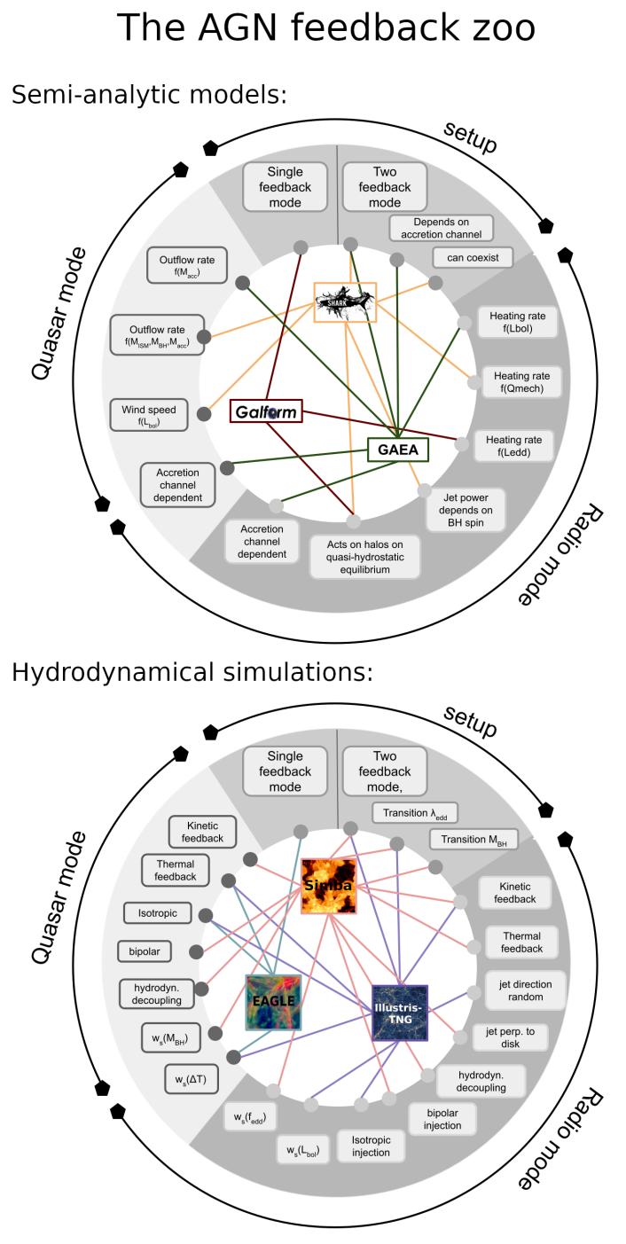
Figure 1: Visualisation of the different decisions made by the SAMs (top) and cosmological hydrodynamical simulations (bottom) employed in this paper regarding their AGN feedback model. At the top, is the setup: whether one or two modes of AGN feedback are invoked. If two modes are invoked, then how one transitions between them is shown. For simplicity we call the two modes of feedback “QSO” and “radio” mode, which generally refer to the radiatively-efficient and inefficient modes of feedback, respectively. For the wheel of decisions for SAMs, in both modes, $f$ represents a function, and its potential parameters are $L_{\rm bol}$, $Q_{\rm mech}$, $L_{\rm edd}$, $M_{\rm acc}$ and $M_{\rm ISM}$, being the BH’s bolometric luminosity, mechanical power, Eddington’s luminosity, accretion rate and the ISM mass, respectively. In the case of hydrodynamical simulations, $w_{\rm s}$ refers to the wind speed and whether this is computed as depending on the BH mass, $w_{\rm s}(M_{\rm BH})$, as a change in temperature, $w_{\rm s}(\Delta\,\rm T)$, as depending on the Eddington ratio, $w_{\rm s}(f_{\rm edd})$, or the bolometric luminosity, $w_{\rm s}(L_{\rm bol})$. These figures visually show which models are more complex given their number of decisions. In the case of SAMs, Galform has the simplest model, while Shark has the most complex one. For hydrodynamical simulations, Eagle has the simplest mode, while Simba has the most complex one. Visualisation was inspired by the method presented in Thorne et al. (2021), see their Fig. 1.

2.2 Cosmological hydrodynamical simulations

For this work we analyse a suite of cosmological hydrodynamical simulations that are publicly available and that simulate large enough cosmological volumes as to contain several dozen massive-quenched galaxies at high redshift. All these simulations include sub-grid models that capture unresolved physics, including (i) radiative cooling and photoheating, (ii) star formation from cold, dense gas, (iii) stellar evolution and chemical enrichment, (iv) stellar feedback, and (v) BH growth and AGN feedback. Similarly to SAMs, for each simulation we describe in some detail the adopted AGN feedback model, which is modelled very differently in each of the three simulations. In general though and in hydrodynamical simulations, the energy associated with AGN feedback is coupled to the gas using “thermal” and “kinetic” approaches (in some cases, a combination of both). Thermal feedback is nominally implemented by heating the relevant gas elements, while kinetic feedback involves directly “kicking” gas elements with a prescribed velocity to generate an outflow. In hydrodynamical simulations no explicit treatment of galaxy mergers and disk instabilities is required, as those naturally arise as the galaxies are evolved.

2.2.1 Eagle

The eagle simulation suite (described in detail in Schaye et al. 2015 and Crain et al. 2015) consists of a large number of cosmological hydrodynamic simulations with different resolutions, cosmological volumes and subgrid models. Eagle was performed using an extensively modified version of the parallel $N$-body smoothed particle hydrodynamics (SPH) code GADGET-3 (Springel, 2005; Springel et al., 2008). Among those modifications are updates to the SPH technique, which are collectively referred to as “Anarchy” (see Schaller et al. 2015 a discussion impact of these changes on the properties of simulated galaxies compared to standard SPH). Eagle used SUBFIND to identify galaxies and that is the catalogue used in this paper.

For AGN feedback, Eagle adopts a single model which comprises a stochastic heating model. Here, gas particles surrounding the BH are chosen randomly and heated by a temperature $\Delta T_{\rm AGN}=10^{8.5}$ K. The rate of energy injection from AGN feedback is computed from the BH accretion rate, and a fixed conversion efficiency of accreted rest mass to energy. In Eagle, particles influenced by feedback (either stellar or AGN) are not decoupled from the hydrodynamics when they receive a temperature boost. Hence, the temperature boost is required to be large as to avoid rapid cooling and dissipation of the feedback energy (see Crain et al. 2015 for details). Because gas particles affected by AGN feedback are chosen at random, the resulting outflow has no preferential direction.

The reference Eagle model used in this work, was calibrated to ensure a good match to the $z=0.1$ galaxy stellar mass function, the sizes of present-day disk galaxies and the BH-stellar mass relation (see Crain et al. 2015 for details on the tuning of parameters).

eagle adopts a Planck Collaboration (2014) cosmology: $\Omega_{\rm m}=0.307$, $\Omega_{\rm b}=0.04825$, $\Omega_{\Lambda}=0.693$, $h=0.6777$, $n_{\rm s}=0.9611$ and $\sigma_{8}=0.8288$. Here, we use the largest Eagle run, which consists of a box of $(100\,\rm cMpc)^{3}$ with an initial number of particles $2\times 1504^{3}$. The initial gas particle mass is $1.81\times 10^{6}\,\rm M_{\odot}$ and the DM particle mass is $9.7\times 10^{6}\,\rm M_{\odot}$.

2.2.2 Illustris-TNG

The Next Generation Illustris simulations, known as Illustris-TNG (Springel et al., 2018; Pillepich et al., 2018), are a collection of cosmological magneto-hydrodynamical simulations conducted using the moving-mesh refinement code AREPO (Springel, 2010; Pakmor et al., 2011; Weinberger et al., 2020). Illustris-TNG used SUBFIND to identify galaxies and that is the catalogue used in this paper.

Illustris-TNG’s AGN feedback model is described in detail in Weinberger et al. (2017) and in short is made up of two modes: at high BH accretion rates feedback is injected in thermal mode within a spherical region around the galaxy; at low BH accretion rates, feedback is injected in a kinetic form (as kinetic winds). In the latter, the direction of the jets is randomised at each time step. The transition between the two AGN feedback modes above is based on a BH-dependent accretion rate (see equation 6 in Weinberger et al. 2017), in a way that the BH accretion threshold below which kinetic feedback switches on increases with increasing BH mass. Terrazas et al. (2020) found that given the conditions at $z=0$, the AGN feedback kinetic mode switches at a BH mass of $\approx 10^{8.2}\,\rm M_{\odot}$. In both of the accretion modes, feedback is injected into surrounding gas cells (the “feedback region”) with no preferential direction, and there is no hydrodynamic decoupling of feedback-affected gas elements.

The free parameters of the Illustris-TNG model were tuned to reproduce the cosmic SFR density evolution, the $z\approx 0$ SMF, and the present-day stellar-to-halo mass relation.

All of the Illustris-TNG boxes assume a Planck Collaboration et al. (2016) cosmology, with $\Omega_{\rm m}=0.31$, $\Omega_{\rm b}=0.0486$, $\Omega_{\Lambda}=0.692$, $h=0.677$, $n_{\rm s}=0.97$ and $\sigma_{8}=0.8159$. In this paper we use the TNG100 run, a box of volume $(75.0\,\rm cMpc/h)^{3}$, an initial gas cell mass of $1.40\times 10^{6}\,\rm M_{\odot}$, and DM particle mass of $7.5\times 10^{6}\,\rm M_{\odot}$.

2.2.3 Simba

Simba (Davé et al., 2019) uses the meshless finite mass (MFM) mode of the GIZMO hydrodynamics code (Hopkins, 2015, 2017), with a gravity solver based on GADGET-3 (Springel, 2005). Galaxies are identified using a friends-of-friends galaxy finder, assuming a spatial linking length of $0.0056$ times the mean inter-particle spacing (equivalent to twice the minimum softening length). The latter is the catalogue used in this paper.

Simba’s AGN feedback model (introduced in Anglés-Alcázar et al. 2017) includes kinetic and thermal feedback. Kinetic feedback is applied to both AGN that are radiatively-efficient and inefficient (the latter is also referred to as “jet” mode). The thermal mode (referred to as “X-ray heating” in Davé et al. 2019) only acts in radiatively-inefficient AGN and in galaxies that are gas poor. In the radiatively-efficient mode, winds with velocities $500-1500\,\rm km/s$ are produced, with the exact wind velocity depending on BH mass (where $v_{\rm wind}=1000\,\rm km/s$ corresponds to a BH mass of $10^{9}\,\rm M_{\odot}$). The jet mode occurs for BHs with masses $\geq 10^{7.5}\,\rm M_{\odot}$ and accretion rates that are $<0.2\,M_{\rm Edd}$, with $M_{\rm Edd}$ is the Eddington rate. Note, however, that the jet-mode builds-up as the Eddington ratio becomes smaller, and peaks in efficiency at $0.02\,M_{\rm Edd}$. The jet-mode can add a velocity boost of up to $7000\,\rm km/s$ additional to the regular wind velocity above. Thus, outflows can be as fast as $8000\,\rm km/s$. Gas is ejected by the jets in a bipolar fashion but with an opening angle of $0$, with the jets being perpendicular to the inner disk. Note that this is different to Illustris-TNG in which the direction of the jets is randomised. The gas affected by jets remains hydrodynamically decoupled for a duration of $10^{-4}\,t_{\rm H}(z)$, where $t_{\rm H}(z)$ is the Hubble time at redshift $z$. The latter allows jets to travel up to $\approx 10$ pkpc before the energy is deposited into the surrounding gas. Gas in the jets is injected at the halo virial temperature.

The free parameters of Simba were tuned to provide a reasonable match to the $z\approx 0$ SMF and the BH-stellar mass relation .

The Simba simulations adopt cosmological parameters $\Omega_{\rm m}=0.30$, $\Omega_{\rm b}=0.048$, $\Omega_{\Lambda}=0.70$, $h=0.68$, $n_{\rm s}=0.97$ and $\sigma_{8}=0.82$. We use the largest Simba simulation box, which consists of a box of volume $(100\,h^{-1})^{3}\,\rm cMpc$, a gas element mass of $1.8\times 10^{7}\,\rm M_{\odot}$, and DM particle mass of $9.7\times 10^{7}\,\rm M_{\odot}$.

The bottom panel of Fig. 1 shows visually the different decisions made by the three hydrodynamical simulations employed in this work. Eagle has the simplest model of the three simulations here, with a single AGN feedback mode, while Simba has the most complex model, with two modes, and a “radio” mode that uses both thermal and kinetic feedback. Note that for Illustris-TNG we say the wind speed is implemented as a temperature increase because in practice the energy is saved until there is enough to kick the gas at high enough speeds, in a similar way to how gas particles are heated to a certain temperature in Eagle. Table 1 shows the cosmological volume and DM particle mass of each of the simulations analysed here.

2.3 Galaxy properties and selection of passive galaxies

Table 1: The cosmological volume, DM particle mass, number of massive-quenched galaxies at $z=3$ ($N_{\rm pass}$), the implied number density of massive-quenched galaxies, $\phi_{\rm pass}$, and the percentage of galaxies with $M_{\star}\geq 10^{10}\rm\,M_{\odot}$ that are quenched at $z=3$ ($f_{\rm pass}$) of each simulation. For the SAMs, we also report in parenthesis the number of central massive-quenched galaxies and their number density. The percentage of passive galaxies in the right-most column for SAMs corresponds to that of central galaxies.

Simulation	volume [$\rm cMpc^{3}$]	$m_{\rm DM}/M_{\odot}$	$N_{\rm pass}$	$\phi_{\rm pass}\,\rm[cMpc^{-3}]$	$f_{\rm pass}$
Shark	$(800)^{3}$	$1.56\times 10^{8}$	$44,257$ ($18,831$)	$\,\,\,\,8.62\times 10^{-5}$ ($3.68\times 10^{-5})$	$5.2$%
GAEA	$(684.93)^{3}$	$1.18\times 10^{9}$	$15,990$ ($12,792$)	$\,\,\,\,1.38\times 10^{-4}$ ($1.1\times 10^{-4}$)	$9.3$%
Galform	$(710.23)^{3}$	$1.33\times 10^{9}$	$12,677$ ($8,846$)	$\,\,\,\,3.54\times 10^{-5}$ ($2.45\times 10^{-5}$)	$3.9$%
Eagle	$(100)^{3}$	$9.7\times 10^{6}$	$35$	$3.5\times 10^{-5}$	$5.5$%
Illustris-TNG	$(110.78)^{3}$	$7.6\times 10^{6}$	$43$	$3.17\times 10^{-5}$	$6.1$%
Simba	$(142.86)^{3}$	$9.7\times 10^{7}$	$36$	$1.13\times 10^{-5}$	$3.6$%

We focus on selecting passive galaxies at $z=3$, as this is a redshift where the simulations analysed here have enough galaxies (at least $30$) and where most of the current observational constraints of massive-quenched galaxies from the JWST are located (see Fig. 3). Unless specified, we show $z=3$ galaxies only.

Throughout this paper we use stellar masses, SFRs and SFR histories of galaxies in the SAMs and hydrodynamic simulations. Below we briefly describe how these quantities are computed:

• Stellar masses ($M_{\star})$: for the SAMs we use the total (remaining) stellar mass (disk plus bulge). For the hydrodynamical simulations we measured stellar masses as the sum of the remaining masses of all the stellar particles enclosed within a sphere of radius $50$ ckpc (comoving kpc) around the centre of potential of each subhalo. Visual inspection of massive galaxies show that this aperture is sufficient to encompass the galaxy while also avoiding potential contamination from substructure.

• SFRs: for the SAMs we use the total SFR averaged over a snapshot (disk plus bulge). Because of the difference time cadence in the SAMs, the SFR at $z=3$ corresponds to the average over the previous $\approx 41$ Myr for Shark, and $\approx 181$ Myr for GAEA and Galform. For the hydrodynamical simulations we compute a recent SFR using the stellar particles that formed in the last $20$ Myr before the output time of interest ($z=3$). In practice, we sum the mass with which stellar particles formed during that period and divide by $20$ Myr.

• BH mass: for the hydrodynamical simulations we save the mass of the most massive BH within a sphere of $10$ ckpc of the centre of potential. For the SAMs, this is well defined and each galaxy has a single value.

• Host halo mass: For Shark, eagle, Illustris-TNG and Simba, we use $M_{\rm 200crit}$ to measure the host halo mass, where this is the mass enclosed by a sphere of mean density $200$ times the critical density of the universe. For Galform instead we use the “D-halo” host halo mass, which is $\approx 1.26$ times higher than $M_{\rm 200crit}$, while for GAEA we use the FOF halo mass, which tends to be $\approx 1.23$ times more massive than $M_{\rm 200crit}$. These factors come from Jiang et al. (2014), and we apply them to scale the halo masses down to an approximate $M_{\rm 200crit}$.

• SFR and stellar mass histories: For the SAMs, we compute the SFR histories by summing the SFRs at each snapshot of all the progenitors of the $z=3$ galaxies. Because of the different number of snapshots, the time cadence is different for the three SAMs. The SFHs are sampled with $100$, $28$ and $16$ timesteps for Shark, GAEA and Galform, respectively. These timesteps correspond to a typical time cadence of $30-40$ Myr for Shark and $100-180$ Myr for GAEA and Galform. For the hydrodynamical simulations, we take all the stellar particles enclosed in the $50$ ckpc sphere described above and bin them in $100$ timesteps of $20$ Myr each using their formation time. We compute the SFR at each timestep in the same way as we do the SFRs above. Similarly, we compute the stellar mass history for galaxies in SAMs by summing the stellar mass formed by each snapshot of all the progenitors of the $z=3$ galaxies. For the hydrodynamical simulations, we sum the $z=3$ stellar particle masses of particles formed by a given point in time.

• Maximum SFR: with the SFR histories above, we extract the maximum SFR each galaxy at $z=3$ had in the past (regardless of when that happens), and refer to that as $\rm SFR_{\rm max}$. For the same time, we also define the maximum sSFR as $\equiv\rm SFR_{\rm max}/M_{\star}(\rm at\,SFR_{\rm max})$, where $M_{\star}(\rm at\,SFR_{\rm max})$ is the stellar mass the galaxy had when it reached $\rm SFR_{\rm max}$. The poorer time cadence in GAEA and Galform is likely to affect $\rm SFR_{\rm max}$ as it would be an average over $\approx 100-180$ Myr, while for the other simulations, $\rm SFR_{\rm max}$ is an average over $\approx 20-40$ Myr. Appendix C shows that although there is an effect of the time cadence, it is not big, and does not change our conclusions.

• Stellar ages: with the stellar mass histories defined, we compute $3$ stellar ages as the lookback time (from $z=3$) to when the $z=3$ galaxies had assembled $50$%, $80$% and $90$% of their stellar mass. We refer to these ages as $\rm age_{50}$, $\rm age_{80}$ and $\rm age_{90}$, respectively.

We test using different spherical apertures for the hydrodynamical simulations, using $10$ ckpc, $30$ ckpc and using twice the half-stellar mass radius, and find little difference in the results presented here. The main difference is that smaller apertures increase slightly the number of passive galaxies, but differences are $<10$%. Note that the $10$ ckpc is similar to the aperture used to measure colours for galaxies with the JWST and HST, which are what is ultimately used to select quenched galaxies at high-z.

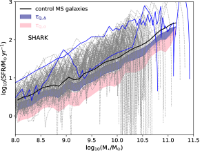
Figure 2: The evolution of 70 randomly selected $z=3$ massive-quenched galaxies in Shark in the SFR-stellar mass plane (individual dotted lines). We highlight two of them with blue lines: one that grows above the main sequence most of its life and that has one quenching period prior to the one that leads to it being quenched at $z=3$; and another that instead moves mostly along the main sequence, bar an early starburst, until there is a big starburst, followed by quenching close to $z=3$. The black, solid line shows the median growth of the control MS sample. We define $\tau_{\rm Q,\Delta}$ as the time a galaxy takes to move through the band while quenching, while $\tau_{\rm Q,\sigma}$ is defined using the pink band instead.

With the defined properties above we select a sample of passive, massive galaxies and a control sample of star-forming galaxies following the criteria below:

• massive-quenched galaxies: are defined as those with $M_{\star}>10^{10}\,\rm M_{\odot}$ and a specific SFR ($\equiv\rm SFR/M_{\star}$) $<10^{-10}\rm\,yr^{-1}$. The latter is a good criterion to select passive galaxies as shown by Franx et al. (2008); Schreiber et al. (2018); we discuss this threshold further in § 3. Table 1 shows the number of selected galaxies in each simulation and the implied number density. For the SAMs, in addition to the selection above, we also require galaxies to be centrals. This is done with the aim of focusing the analysis around the effect of AGN feedback. Note that Shark predicts more passive satellite galaxies than GAEA and Galform due to the dynamical friction timescale employed (Poulton et al., 2021), which allows for a much longer survival timescale of satellite galaxies.

• Control sample: in order to have a reference point to compare our massive-quenched galaxy sample, we select a sample of massive-active galaxies. To do so, we first compute the median sSFR, $\rm sSFR_{\rm MS}$ (with MS referring to “main sequence”) of all galaxies with $M_{\star}>10^{10}\,\rm M_{\odot}$ and sSFR$>10^{-9.9}\,\rm yr^{-1}$ at $z=3$, and then select all galaxies with $M_{\star}>5\times 10^{10}\,\rm M_{\odot}$ and $\rm sSFR>0.63\,sSFR_{\rm MS}$ (the $0.63$ is equivalent to requiring galaxies to have a sSFR above $\rm sSFR_{\rm MS}$ minus 0.2 dex). For the control sample, we also compute SFR histories. We refer to this sample as “control MS sample”.

With a control sample defined, we can also compute a main sequence in the SFR-$M_{\star}$ plane internal to each simulation as follows. We use the growth of galaxies in the control sample in the SFR-$M_{\star}$ to measure a median SFR, $\rm\langle SFR\rangle$, and a standard deviation, $\sigma_{\rm MS}$, in bins of stellar mass (which we show later in § 4.2 in Fig. 10 as black solid and dotted lines, respectively) and define this relation as our main sequence. We can then compute a distance to the main sequence, $\Delta_{\rm MS}=\rm log_{10}(SFR/\langle SFR(M_{\star})\rangle$, with $\rm SFR$ and $M_{\star}$ being the SFR and $M_{\star}$ at any point in the history of the massive-quenched galaxy sample. Because each simulation also predicts different widths of the main sequence, we also analyse the distance to the main sequence in units of the main sequence’s standard deviation, $\Delta_{\rm MS}/\sigma_{\rm MS}$, where a value of $1$ indicates $1\sigma$ deviation from the main sequence. Appendix A shows that this way of defining a main sequence and deviations to the main sequence is similar to measuring the main sequence at individual redshifts and using those to measure a distance to the main sequence (which is the more common way of doing it).

With the distance to the main sequence defined at all points in the history of the $z=3$ massive-quenched galaxies, we move to quantifying quenching timescales. Defining quenching timescales from the trajectory of galaxies in the SFR-stellar mass plane involves applying some arbitrary distance to the main sequence and measure how long it takes for a galaxy to fall below some thresholds of $\Delta_{\rm MS}$ (e.g. Wright et al. 2019). Alternatively, using colours makes for a clearer definition as the blue cloud and red sequence are quantifiable populations in the colour-magnitude diagram (e.g. Wright et al. 2019; Bravo et al. 2022, 2023). The drawback of the latter approach is the fact that there is no clear red sequence in place at $z=3$ yet in many of the simulations employed here (e.g. Trayford et al. 2016). Hence, we decide to define quenching timescales based on the distance to the main sequence in the two following ways:

• $\tau_{\rm Q,\Delta}$: We define two points of interest in $\Delta_{\rm MS}$ based on previous literature: a value of $-0.3$ to $-0.5$ indicates the point when the galaxy leaves the main sequence, and $-1$ to $-1.3$ when the galaxy is considered quenched (e.g. Wright et al. 2019; Bluck et al. 2020; Mun et al. 2024). Here we measure the time it takes for the galaxies to go from $\Delta_{\rm MS}=-0.3$ to $-1$ and refer to this time as $\tau_{\rm Q,\Delta}$. If galaxies have several quenching periods, we take only the last one (i.e. the one closest to a lookback time of $0$). We tested different values within the ranges above and find that the results remain qualitatively the same.

• $\tau_{\rm Q,\sigma}$: The measurement above fails at considering the fact that each simulation predicts different widths of the main sequence. For example, in Illustris-TNG the main sequence is extremely tight, with a standard deviation $\approx 0.1$ dex, while in Shark the dispersion is larger, $\approx 0.25$ dex. In this context, a $\Delta_{\rm MS}=-0.3$ in Illustris-TNG implies a significant deviation from the main sequence, while in Shark such galaxy would be just leaving the main sequence. Hence, we also measure a timescale using $\Delta_{\rm MS}/\sigma_{\rm MS}$ and thresholds of $-1$ and $-2$; i.e. the time it takes the galaxy to go from a main sequence deviation of $1\sigma$ to $2\sigma$ below the main sequence. The exact values are again arbitrary, but we find that varying these values a bit does not impact the results significantly.

Fig. 2 shows visually how we measure $\tau_{\rm Q,\Delta}$ and $\tau_{\rm Q,\sigma}$, using $70$ randomly selected $z=3$ massive-quenched galaxies. $\tau_{\rm Q,\Delta}$ is the time a galaxy takes between entering and leaving the blue band, while for $\tau_{\rm Q,\sigma}$ this corresponds to moving through the pink band. We also highlight two galaxies, with the aim of highlighting the diversity of trajectories of galaxies in this plane.

Finally, we note that the simulations adopt slightly different cosmologies. Those adopted by Shark, Eagle, Illustris-TNG and Simba are very similar, and stellar masses and SFRs are expected to differ only by $1$% due to the differing cosmologies (as indicated by the differences in their $h$ parameters). This is larger for GAEA ($\approx 9$%) and Galform ($\approx 5$%). These differences are much smaller than those produced by the baryon physics included in each model, so we neglect them.

3 Number densities and stellar mass function of high-z massive quiescent galaxies

3.1 Number density of massive-quenched galaxies at $2<z<5$

Figure 3: Number density of passive massive galaxies selected based on two stellar mass thresholds, $M_{\star}>10^{10}\,\rm M_{\odot}$ (thick lines) and $M_{\star}>10^{10.5}\,\rm M_{\odot}$ (thin lines) and three sSFR thresholds, $<10^{-10}\,\rm yr^{-1}$ (solid lines), $<5\times 10^{-11}\,\rm yr^{-1}$ (dashed lines) and $<10^{-11}\,\rm yr^{-1}$ (dotted lines), as labelled, between $2\leq z\leq 5$. This is shown for the $6$ simulations being analysed; the SAMs: Shark  GAEA, and Galform; and the hydrodynamical simulations: Eagle, Illustris-TNG, and Simba, as labelled in each panel. Masses and SFRs are measured as described in § 2.3. For the redshift bins with $0$ passive galaxies, we use an arbitrary low number density of $10^{-9}\,\rm cMpc^{-3}$. Observational estimates are also shown: in grey symbols (pre-JWST results) are from Straatman et al. (2014); Schreiber et al. (2018); Merlin et al. (2019); Girelli et al. (2019); Carnall et al. (2020); Weaver et al. (2023); Gould et al. (2023), and green symbols (JWST results) are from Nanayakkara et al. (2024); Carnall et al. (2023a); Valentino et al. (2023); Alberts et al. (2023), as labelled in each panel.

Figure 4: Top panel: Stellar mass function of galaxies at $z=3$ selected to have a $\rm sSFR<10^{-10}\,\rm yr^{-1}$ in the $6$ different simulations analysed, as labelled. We show Poisson errorbars with shaded regions to demonstrate that the differences between simulations are significant. Observations from Weaver et al. (2023) for passive galaxies are shown in symbols for redshifts around $z=3$. The latter sample was selected using colour-colour selection (see text for details). The vertical dotted line marks the approximate stellar mass above which observational estimates of the SMF are reliable according to Weaver et al. (2023). Bottom panel: as in the top panel but after convolving stellar masses with Gaussian-distributed errors with a width of $0.25$ dex.

Fig. 3 shows the predicted number density of massive-quiescent galaxies at $2\leq z\leq 5$ in the $6$ simulations analysed. We show this using two thresholds of stellar mass, $M_{\star}>10^{10}\,\rm M_{\odot}$ (thick lines) and $M_{\star}>10^{10.5}\,\rm M_{\odot}$, and three of sSFR, $<10^{-10}\,\rm yr^{-1}$, $<5\times 10^{-11}\,\rm yr^{-1}$ and $<10^{-11}\,\rm yr^{-1}$. The idea of using these different thresholds is to capture the range of values adopted in the literature. Most works select passive galaxies based on their position in the UVJ colour-colour plane, but the equivalent sSFR selection is unclear. Weaver et al. (2023) argue that this colour selection is roughly equivalent to requiring $\rm sSFR<10^{-11}\,\rm yr^{-1}$ (see also Belli et al. 2019), while Schreiber et al. (2018) argue this is equivalent to a $\rm sSFR<10^{-10}\,\rm yr^{-1}$. Given the uncertainty, we show three selections spanning this sSFR range. As for the stellar mass, observations of passive high-z galaxies have started to push down to $10^{9.5}\,\rm M_{\odot}$ (e.g. Valentino et al. 2023), but because the vast majority of the samples are composed of galaxies with $M_{\star}\gtrsim 10^{10}\,\rm M_{\odot}$, we focus on two bins above that.

The predicted number densities are very different between different simulations. Focusing first on Shark, we see that the sSFR threshold has almost no effect, due to passive galaxies being very passive (i.e. being many dex below the main sequence). Conversely, the stellar mass threshold has a significant impact, with the number density decreasing by $\gtrsim 1$ dex in the sample of $M_{\star}>10^{10.5}\,\rm M_{\odot}$ galaxies. GAEA behaves very similarly, but with a lesser difference between the two stellar mass bins, specially at $z<3$. The latter is due to GAEA producing a less steep high-mass end of the stellar mass function of passive galaxies compared with Shark (visible in Fig. 4).

In Eagle and Galform, both the stellar mass and sSFR threshold have an important effect on the number density. This shows that in these simulations there is a large population of massive galaxies that are moderately quenched (i.e. $10^{-11}\,\rm yr^{-1}\lesssim sSFR\lesssim 10^{-10}\,yr^{-1}$). This is very clearly seen later in § 4.2 in Fig. 10. For the most massive bin in Eagle, we see there are no galaxies with $\rm sSFR<10^{-11}\,yr^{-1}$ ($\rm sSFR<5\times 10^{-10}\,yr^{-1}$) at $z\gtrsim 2.5$ ($z\gtrsim 3$).

Simba shows number densities of passive galaxies that are only mildly dependent on both stellar mass and sSFR. For instance, it displays a stronger dependence on sSFR than Shark and GAEA but much weaker than Eagle and Galform. Illustris-TNG behaves very differently with the number density of passive galaxies of any mass and sSFR threshold falling off sharply at $z\gtrsim 3.5$ with no quenched massive galaxies at $z\geq 4$. At lower redshifts, the sSFR threshold makes a negligible difference as in Shark and GAEA, while the stellar mass threshold only makes a mild difference at $z\lesssim 3.5$. This shows that in Illustris-TNG these quenched galaxies are very massive and very quenched.

In addition to the simulations predicting quite different number densities of massive-quenched galaxies, they also predict very different fractions of passive galaxies ($f_{\rm pass}$; see Table 1), with differences of a factor of $\approx 3$. GAEA predicts the highest fraction ($9.2$%) and Simba the lowest one ($3.6$%). Coincidentally, these two simulations predict a similar number density of massive-quenched galaxies at $z\approx 3-5$, and hence the different $f_{\rm pass}$ imply that these simulations predict very different number densities of massive galaxies.

The observations shown in Fig. 3 display large variations and when focusing on results using JWST observations, we find that all the simulations prefer the lower number densities that are obtained using the NUVU-VJ plane, which is expected to be more robust (i.e. having fewer contaminants) than the classic UVJ selection (Gould et al., 2023). This uses three colours instead of two and a probabilistic method to assign galaxies to the star-forming and passive populations.

At $z\gtrsim 4.5$ only Shark, Simba and GAEA produce quenched galaxies in reasonable numbers; however they tend to have $10^{10}\,\rm M_{\odot}\lesssim M_{\star}\lesssim 10^{10.5}\,M_{\odot}$ which may be too low compared to the derived stellar masses in observations. Note that Szpila et al. (2024) presented number densities of massive-quenched galaxies at high-z using Simba-C, an improved version of Simba with an updated chemical evolution model and tweaked feedback parameters. Those number densities are similar to the ones we obtain using Simba, and hence we do not expect other results presented here for Simba to be too dissimilar to what is seen in Simba-C.

In addition to the SAMs we study here, Vani et al. (2024) presented an analysis of the L-galaxies semi-analytic model in three different flavours and found that all of them struggled to produce enough massive-quenched galaxies at $z\gtrsim 1.5$. Remus & Kimmig (2023) show that in the hydrodynamical simulation Magneticum, the number density of massive-quenched galaxies matches relatively well the observations at $z\approx 3-4$. This is also shown in Fig. 15 for a single stellar mass and sSFR thresholds that are comparable to the ones used in Fig. 3. Magneticum predicts the highest massive-quenched galaxy number density at $z=3-4$ of the simulations analysed here, but it also massively over-predicts the number density of those galaxies at slightly lower redshift $z=2-3$, likely due to a combination of overly efficient AGN feedback and resolution effects affecting the galaxies with stellar masses close to $10^{10}\,\rm M_{\odot}$ (see Appendix B for a discussion).

Thus, the difficulty in reproducing the frequency of massive-quenched galaxies from cosmic dawn to noon is a very pervasive problem in modern galaxy formation simulations.

3.2 The $z=3$ stellar mass function of quenched galaxies

The top panel of Fig. 4 shows the $z=3$ stellar mass function of passive galaxies selected to have $\rm sSFR<10^{-10}\,\rm yr^{-1}$. The observations correspond to those of Weaver et al. (2023), where passive galaxies were selected from the NUVrJ plane. Shark, Eagle and Galform tend to produce the correct number density of passive galaxies with $10^{10}\rm\,M_{\odot}\lesssim M_{\star}\lesssim 10^{10.6}\,\rm M_{\odot}$ but predict too few passive galaxies of higher masses, while GAEA’s agreement with observations extends to $M_{\star}\approx 10^{11}\,\rm M_{\odot}$; albeit also producing too few galaxies above that mass threshold. Simba and Illustris-TNG produce enough massive-quiescent galaxies with $M_{\star}\gtrsim 10^{11}\,\rm M_{\odot}$ but too few at lower stellar masses compared with observations. This shows that the suite of simulations here agree with observations in different regimes. The exact cause of this is the way AGN feedback is modelled and we discuss this in § 4.3.

To demonstrate the effect uncertainties in stellar masses can have in the stellar mass function, we show in the bottom panel of Fig. 4 the mass functions after we convolve the stellar masses in each simulation with errors that are Gaussian-distributed with a width of $0.25$ dex. The tension seen between simulations that underpredict the abundance of passive galaxies with $M_{\star}\gtrsim 10^{11}\,\rm M_{\odot}$ and the observations, is greatly diminished (clearly seen for Shark, Galform and GAEA). The same can be said for the tension at $M_{\star}\lesssim 10^{10.5}\,\rm M_{\odot}$ seen in Simba and Illustris-TNG, but because the stellar mass function at those masses is less steep, the effect of a random error is less pronounced.

The $0.25$ dex width of error above is informed by the reported errors from spectral energy distribution (SED)-derived stellar masses at $z<0.1$ of Robotham et al. (2020). Robotham et al. (2020) computed these masses using $27$ bands covering from the FUV to the FIR of galaxy SEDs and found typical errors of $0.2$ dex. At $z=3$ the stellar mass uncertainties are likely larger due to the more limited wavelength range of galaxy SEDs and redshift uncertainties, to mention a few (see Pacifici et al. 2023 for a comprehensive study of systematic effects in the derivation of galaxy properties from SED fitting). In fact, Wang et al. (2024) show that excluding the JWST mid-IR bands in the derivation of stellar masses can bias the inferences high by even an order of magnitude (which mostly affect galaxies at $z>3$). Hence, what is shown in the bottom panel of Fig. 4 is likely a lower limit of the effect of uncertainties in the stellar mass function. Thus, quantifying systematic errors in the derived stellar masses and SFRs of galaxies from observations is paramount to provide stringent constraints to the simulations.

Another source of difference between simulations and observations could be possible contamination of the colour-colour selection employed by Weaver et al. (2023) in the process of constructing the SFMs of passive galaxies. Lagos et al. (2024) showed, using Shark, that the NUVrJ selection can lead to significant contamination from massive, star-forming galaxies at $z\gtrsim 2$. At lower redshifts, they found little contamination. Lagos et al. (2024), however, showed that even after applying the NUVrJ selection to Shark galaxies, the increased number density of passive galaxies selected by their colour was not enough to bring the simulation into agreement with Weaver et al. (2023) at $z=3$. De Lucia et al. (2024) using GAEA also explored the performance of the NUVrJ selection in their simulation and found that up to $z\approx 3$ it performs well, without significant contamination. Akins et al. (2022) explored the performance of the UVJ colour selection instead in Simba up to $z=2$ and found that overall it selected the expected population of passive galaxies. The overall conclusion is that at $z=3$ is still unclear how much contamination there may be in the colour-selected samples of passive galaxies, but it is unlikely to be large enough as to bring the models into agreement with observations.

Another potential source of difference between simulations and observations is cosmic variance. The volumes of the three hydrodynamical simulations used here are small; at $z\approx 3$ and using the cosmic variance calculator of Driver & Robotham (2010), we find a cosmic variance of $\approx 25$%. This is still a lot smaller than the differences seen between simulations, which tend to be of factors of several.

3.3 The stellar-halo mass relation of quenched galaxies at $z=3$

Figure 5: The stellar-to-halo mass ratio in units of $\Omega_{\rm b}/\Omega_{\rm m}$ as a function of halo mass for the $z=3$ massive-quenched galaxies in each simulation, as labelled. Lines with shaded regions show the medians and $16^{\rm th}-84^{\rm th}$ percentile ranges, respectively. We use adaptive bins to ensure a number of galaxies per bin $\geq 10$. The horizontal dotted lines show baryon collapse efficiencies of $10$%, $30$% and $50$% for reference.

The different SMFs of quenched galaxies in the $6$ simulations of Fig. 4 naturally points to potentially different stellar-halo mass relations between the simulations. The large stellar masses derived for massive-quenched galaxies in observations (of even of up a few $10^{11}\,\rm M_{\odot}$) have been used to argue that to form these galaxies (or at least the most massive) very efficient baryon to stellar mass conversion is required (a.k.a. “baryon collapse efficiency”; e.g. Glazebrook et al. 2017; Carnall et al. 2024). In fact, for extreme galaxies, such as ZF-UDS-7329 (Glazebrook et al., 2024), baryon collapse efficiencies as high as $\approx 50-100$% have been suggested (Carnall et al., 2024).

Fig. 5 shows the stellar-to-halo mass ratio as a function of halo mass for massive-passive galaxies at $z=3$ in each simulation. We normalise the y-axis by $\Omega_{\rm b}/\Omega_{\rm m}$ internal to each simulation to turn it into baryon collapse efficiency. We highlight three efficiencies. The $10$% is the one preferred by most simulations at the lowest halo masses, while $30$% and $50$% are motivated by Glazebrook et al. (2017); Carnall et al. (2024) suggesting those values are required to explain some extremely massive and early-forming quenched galaxies at $z=3-4$.

The lack of intermediate-mass galaxies in Simba and Illustris-TNG translate into those simulations having higher baryon collapse efficiencies compared to the other ones by a factor of $\approx 2$. For Simba and Illustris-TNG, the median baryon collapse efficiency is $\approx 0.22$, while for eagle, Shark, GAEA and Galform is $0.13$, $0.049$, $0.037$ and $0.057$, respectively. Hence, between the extremes (Illustris-TNG and GAEA), there is a large difference of a factor of $\approx 5.8$ in baryon collapse efficiency. The results here are pointing to efficiencies $\gtrsim 20$% being required for quenched galaxies to reach stellar masses of $\gtrsim 10^{11}\rm M_{\odot}$ at $z=3$, as the simulations that have lower efficiencies generally fail to produce enough of those massive galaxies. The larger range of probed halo masses in Shark, GAEA and Galform is likely a result of the much larger cosmological volumes compared with the three hydrodynamical simulations used here.

In general, we find that the simulations prefer baryon collapse efficiencies below $30$%, and for the most massive halos, $\gtrsim 10^{12.7}\,\rm M_{\odot}$, efficiencies $<10$% are overall preferred.

4 The star formation histories of high-z massive quiescent galaxies

We study the SFHs of massive-quenched galaxies selected at $z\approx 3$ in $6$ simulations and separate the analysis between when galaxies are forming stars actively (§ 4.1), and when quenching began (§ 4.2). In § 4.3, we connect the differences and similarities seen among simulations with the implementation of AGN feedback in each case.

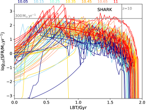
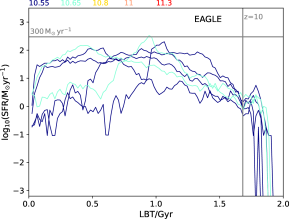
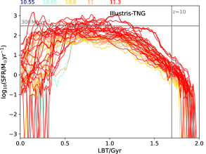
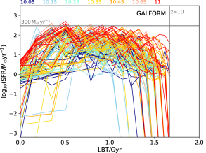
Figure 6: SFR histories for galaxies in the Shark  Eagle, GAEA, Illustris-TNG, Galform, and Simba galaxy formation simulations, as labelled in each panel, selected at $z=3$ to be massive and passive (see § 2.3 for details on the selection). The colour of the lines indicates the stellar mass bins (in units of $\rm M_{\odot}$): $10^{10}-10^{10.1}$, $10^{10.1}-10^{10.2}$, $10^{10.2}-10^{10.3}$, $10^{10.3}-10^{10.4}$, $10^{10.4}-10^{10.5}$, $10^{10.5}-10^{10.75}$, $>10^{10.75}$ (as indicated by the mid bin mass in each bin at the top of each panel). For reference, we show with as a horizontal line a $\rm SFR=300\,\rm M_{\odot}\,yr^{-1}$, and as a vertical line the lookback time corresponding to $z=10$. For EAGLE, Illustris-TNG and Simba we show all the massive-quenched galaxies, while for Shark, GAEA and Galform we only show 10 randomly chosen galaxies in each mass bin, to avoid overcrowding the figures.

4.1 The rise in the star formation rate of massive-quenched galaxies

4.1.1 The SFHs of $z=3$ massive-quenched galaxies

Fig. 6 shows the SFHs of massive-quenched galaxies selected at $z=3$ of all the simulations analysed. We remind the reader that the SFHs are computed by summing the contribution of all progenitors (see § 2.3 for more details). To avoid overcrowding the figure, we only show $10$ randomly selected galaxies per stellar mass bin for the SAMs (Shark, GAEA and Galform) given their very large number of quenched galaxies (see Table 1), while for Eagle, Illustris-TNG and Simba we show all the predicted $z=3$ massive-quenched galaxies. Below we pay especial attention at the predicted SFHs at $z\approx 10$, $z\approx 7$, and $z\approx 4-5$. The justification for this is that many observations of galaxies with relatively high SFRs at $z>10$ are being reported (e.g. Bunker et al. 2023); $z\approx 7$ is considered a typical star formation epoch (e.g. Nanayakkara et al. 2024); and because evidence suggest the peak SFR of $z=3$ massive-quenched galaxies happens at $z=4-5$ (e.g. Valentino et al. 2020; Manning et al. 2022).

Visual inspection of these SFR histories show that Shark and Galform are the models producing the highest SFRs at $z\geq 10$ with values as high as $\approx 50\,\rm M_{\odot}\,yr^{-1}$ (consistent with what has been found by the JWST in Bunker et al. 2023; Castellano et al. 2023; Carniani et al. 2024), while all the other simulations predict SFRs $<10\,\rm M_{\odot}\,yr^{-1}$ at $z\gtrsim 10$. The number density of these progenitors at $z=10$ with $\rm SFR>50\,\rm M_{\odot}\,yr^{-1}$ in Shark and Galform is $2.8\times 10^{-7}\,\rm cMpc^{-3}$ and $7\times 10^{-8}\,\rm cMpc^{-3}$, respectively. Note that for Galform the highest redshift at which we sample the SFHs is $z=10.07$ due to higher redshifts being unavailable in this database. However, from the $z=10.07$ output it is already clear that the progenitors of the $z=3$ massive-quenched galaxies in Galform can have very high SFRs.

Part of the difference between Shark and Galform and the other simulations is the overall larger volumes simulated (although the same large volume is simulated by GAEA), but that is not the whole story. For example, passive galaxies that at $z=3$ have stellar masses $\approx 10^{10.5}\,\rm M_{\odot}$ in Shark and Galform have a median SFR at $z=10$ of $\approx 6.1\,\rm M_{\odot}\,yr^{-1}$ and $\approx 4.1\,\rm M_{\odot}\,yr^{-1}$, respectively; while in GAEA and Eagle (the two simulations having massive-quenched galaxies of those masses at $z=3$) the medians are $\approx 0.9\,\rm M_{\odot}\,yr^{-1}$ and $\approx 1.3\,\rm M_{\odot}\,yr^{-1}$, respectively. The reason for this difference likely resides in the higher star formation efficiency (i.e. the conversion from molecular gas to SFR surface density) Shark and Galform assume for star formation that is driven by galaxy mergers or disk instabilities. In the case of Shark, this is $15$ times more efficient at converting molecular gas into stars compared to star formation happening in galaxy disks, while in Galform this merger or disk instability-driven star formation has an efficiency that is inversely proportional to the bulge dynamical timescale, which tends to give much higher gas-to-stars conversion efficiencies than the disk star formation. Eagle assumes instead a fixed efficiency per unit gas density, while GAEA has very little star formation activity associated with the starburst mode (i.e. driven by galaxy mergers in their case) and hence in the practice is assuming a close to universal molecular-to-SFR surface density conversion efficiency.

Illustris-TNG and Simba produce preferentially very massive-quenched galaxies, with $z=3$ stellar masses $\gtrsim 10^{11}\,\rm M_{\odot}$. These galaxies, however, only have modest SFRs with a median at $z=7$ of $\approx 13\rm\,M_{\odot}\,yr^{-1}$ in Illustris-TNG and $\approx 7.5\rm\,M_{\odot}\,yr^{-1}$ in Simba. Similarly massive galaxies in Shark and Galform have a median SFR at $z=7$ of $33\rm\,M_{\odot}\,yr^{-1}$ and $30\rm\,M_{\odot}\,yr^{-1}$, respectively; while GAEA is similar to Illustris-TNG with a median of $12\,\rm\,M_{\odot}\,yr^{-1}$, respectively. Eagle does not produce such massive galaxies in its volume.

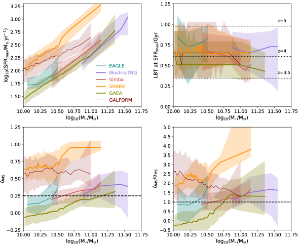
Figure 7: Top-left panel: maximum SFR achieved by the $z=3$ passive, massive galaxies (at any point of their history) as a function of the $z=3$ stellar mass in each of the $6$ simulations, as labelled. Lines with shaded regions show the medians and the $16^{\rm th}-84^{\rm th}$ percentile ranges, respectively. We use adaptive bins to ensure a reasonable number of galaxies per bin. Top-right panel: as in the top-left panel but for the lookback time at which SFR_max happens. Here we show with horizontal lines three different redshifts, as labelled (noting that the cosmologies of the simulations are not exactly the same, but similar enough to use these lines as guidance). Bottom-left panel: Distance to the main sequence (i.e. $\rm log_{10}(sSFR/sSFR_{\rm MS})$; see § 2.3), defined at the point of the maximum SFR of the $z=3$ massive-quenched galaxies as a function of the $z=3$ stellar mass. The dashed line shows the point at which galaxies are at $0.25$ dex above the main sequence. Bottom-right panel: As in the bottom-left panel but for the distance to main sequence in units of the width of the main sequence (measured as the standard deviation of the SFR-stellar mass relation at the point of the maximum SFR; see dotted lines in Fig. 10). The dashed line shows the point at which galaxies are $1\sigma$ above the main sequence.

An interesting difference between simulations is when do $z=3$ massive-quenched galaxies appear for the first time in the simulations. In Shark, Eagle, and Illustris-TNG, the vast majority (if not all) the massive-quenched galaxies appear for the first time at $z>10$, while in Simba, GAEA and Galform there is a large fraction that start forming at $z<10$. Galform, GAEA and Simba predict that $89$ %, $33$% and $44$% of the $z=3$ massive-quenched galaxies appear for the first time in the outputs at $z<10$. In Shark, this happens $1.6$% of the time, while in Eagle and Illustris-TNG it does not happen.

Figure 8: The median and $16^{\rm th}-84^{\rm th}$ percentile range of the SFHs of $z=3$ massive-quenched galaxies are shown with solid lines and shaded regions, respectively, in each simulation, as labelled in each panel. This is shown for massive-quenched galaxies at $z=3$ with $M_{\star}>10^{10.8}\,\rm M_{\odot}$. Eagle has no galaxies of that mass so it is not shown. We also show the derived SFH of the galaxy presented in de Graaff et al. (2024) and the medians of the $6$ galaxies from Nanayakkara et al. (in preparation; referred to as N+24b in the figure), and $4$ galaxies from Carnall et al. (2024), as labelled, that satisfy the same stellar mass cut. Note that for the sample in Nanayakkara et al. (in preparation) we show the inferred SFHs using two different stellar population synthesis models (Miles and C3K), to exemplify systematic uncertainties.

Valentino et al. (2020); Manning et al. (2022) suggest that potential progenitors of $z=3-4$ massive-quenched galaxies are starburst galaxies at $z=4-5$ with SFRs from a few $\approx 100\,\rm M_{\odot}\,yr^{1}$ to $\gtrsim 1000\,\rm M_{\odot}\,yr^{-1}$, based on the latter having a similar number density to the former. Similarly high SFRs are inferred from the spectral fitting of $z=3-4.5$ massive-quenched galaxies at their peak (e.g. Valentino et al. 2020; Glazebrook et al. 2024; Carnall et al. 2024; de Graaff et al. 2024). Such high SFRs are regularly seen in the progenitors of $z=3$ massive-quenched galaxies in Shark and Illustris-TNG, but are rare or non-existent in the other simulations (see also the top-left panel of Fig. 7). Hence, if the evolutionary link between highly star-forming galaxies at $z=4-5$ and $z=3$ passive galaxies is confirmed, it would pose a significant challenge to some of the simulations analysed here.

4.1.2 Tracking the most intense star formation period of $z=3$ massive-quenched galaxies

Fig. 7 shows the relation between $\rm SFR_{\rm max}$ and the $z=3$ stellar mass of the massive-quenched galaxies. We see that at fixed stellar mass, Shark is the simulation producing the highest SFR peak, followed by Galform; while GAEA and Illustris-TNG produce the lowest SFR peaks. Even though the poorer time cadence of GAEA and Galform plays a role in the differences seen (see Appendix C for details), this is not the whole story. In fact, GAEA and Galform have a similar time cadence, but the latter produces much higher $\rm SFR_{\rm max}$ than the former. Overall, Eagle, Simba, GAEA and Illustris-TNG produce a similar $\rm SFR_{\rm max}$-stellar mass relation. The bottom panels of Fig. 7 show the median and scatter of $\Delta_{\rm MS}$ and $\Delta_{\rm MS}/\sigma_{\rm MS}$ at the time of $\rm SFR_{\rm max}$ in each simulation. We see that $\rm SFR_{\rm max}$ corresponds to starburst episodes in Shark, Galform, Simba and Illustris-TNG (i.e. show a high deviation from the main sequence, with the main sequence defined internally to each simulation). In Eagle and GAEA only the most massive galaxies, $\gtrsim 10^{10.35}\,\rm M_{\odot}$ and $\gtrsim 10^{11}\,\rm M_{\odot}$, respectively, appear to be starbursting when they reach $\rm SFR_{\rm max}$.

The top-right panel of Fig. 7 shows the lookback time to $\rm SFR_{\rm max}$. The figure shows that in Shark, Eagle, Simba, Illustris-TNG and Galform $\rm SFR_{\rm max}$ happens preferentially between $z\approx 4-5$ (highlighted by the horizontal lines), while in GAEA $\rm SFR_{\rm max}$ happens at slightly lower redshifts, $z\approx 3.5-4$. Thus, most of the simulations predict the progenitors of the $z=3$ massive-quenched galaxies being highly star-forming at $z\approx 4-5$ in qualitative agreement with the conclusions of Valentino et al. (2020); Manning et al. (2022). However, it is clear that Shark and Galform produce much more intense starbursts than the other simulations. Note that this does not mean that most of the growth of these massive-quenched galaxies happens in the starburst mode (i.e. above the main sequence), but simply that at their peak SFR, they are above the main sequence. Later, we show in Fig. 10 that in fact on average galaxies grow along the main sequence in the SFR-stellar mass plane.

4.1.3 Comparing the predicted SFHs with observations

Fig. 8 shows the median SFHs of massive-quenched galaxies in all the simulations that have stellar masses $>10^{10.8}\,\rm M_{\odot}$ and compares with observationally-derived SFHs. This stellar mass cut is chosen to match the range of most of the available JWST spectroscopic observations. We do not show Eagle here as there are no galaxies in the relevant stellar mass range.

Shark produces the shortest and more pronounced starburst of all the simulations. Simba and GAEA produce the latest forming galaxies, with a peak at a lookback time of $\approx 0.45$ Gyr (compared with peaks at $\approx 0.75$ Gyr for Shark and Illustris-TNG). Galform produces two periods of intense star formation for these galaxies but with the latest one being more pronounced. The figure also shows observationally-derived SFHs from JWST spectroscopy of massive-quenched galaxies of the same stellar mass range as the simulation samples from de Graaff et al. (2024), Carnall et al. (2024) and Nanayakkara et al. (in preparation). The data for Carnall et al. (2024) and Nanayakkara et al. (in prep) correspond to the median of $4$ and $6$ massive-quenched galaxies selected at $z\approx 3-4$, respectively, while the de Graaff et al. (2024) result represents a single galaxy at $z\approx 4.9$. Note that we do not include in the comparison of Fig. 8 the galaxy ZF-UDS-7329 (Glazebrook et al., 2024), as it appears to be an outlier of the bulk of the massive-quenched galaxies with a much earlier formation time.

Of all the simulations, Shark appears to produce the highest peak that resembles better the observationally-derived SFHs. Illustris-TNG, Galform and Simba produce a lower median SFH than observations, but their $84^{\rm th}$ percentile distribution is largely consistent with observations. GAEA on the other hand seems to produce SFHs that are too extended and do not reach the high SFRs derived from spectroscopy. In any case, the current inferences suffer from large systematic uncertainties. de Graaff et al. (2024) show that the peak of the SFH moves significantly if different metallicities are preferred, while Nanayakkara et al. (in preparation) show that the adopted single population synthesis model impacts the recovered SFH, as shown in Fig. 8. Increasing the sample sizes in the observations is crucial to start using the inferred SFHs as stringent constraints on the simulations. This will be possible in the near future.

4.1.4 Single or multiple starburst periods in the SFHs of $z=3$ massive-quenched galaxies

A challenge in observations has been to determine the best way to fit the SFH of massive-quenched galaxies; e.g. whether to use non-parametric SFHs or adopt some function to describe the shape of the SFH. We attempt to shed light into this problem by investigating whether the predicted SFHs can be easily fit with a simple function that displays a unique SFR peak, or whether they have complex enough SFHs that a simple function cannot describe them. In order to determine this, we fit a skewed Gaussian function to every galaxy’s SFH using Highlander, which is the preferred SFH function used to fit galaxies with ProSpect (Robotham et al., 2020). In Appendix D we provide details of the function, the fits and show examples of the individual SFHs and their fits. We calculate a goodness of fit based on the normalised model to data difference, and use those values to select galaxies that are candidates for having clear multiple episodes of starburst activity (which we define as clear unrelated peaks in the SFH).

We then visually inspect the galaxies that were selected as candidates for multi-starbursts and find that a simple threshold in the goodness of fit works very well in Illustris-TNG, Simba and GAEA to isolate galaxies with multiple starbursts. However, in Shark, Eagle, and Galform galaxies with short-duration starbursts are also poorly fit, so a post-processing step is applied to reclassify those as being uni-modal.

Table 2 shows the fraction of galaxies in each simulation displaying clear multiple starburst episodes. The fractions change dramatically between simulations. Eagle and GAEA have the smallest fractions, $\approx 5$%. Conversely, Shark, Galform and Illustris-TNG have about half of the $z=3$ massive-quenched galaxies displaying multiple starbursts. Simba is in between these extremes. Studying the stellar mass of the galaxies with multiple starbursts, we do not find any specific trend; the well-fit vs the badly-fit galaxies having similar masses. The only exception is Simba, in which the best fit SFHs tend to be the most massive galaxies.

The results here are not applicable to lower redshifts. In fact, using Shark, Bravo et al. (2022) show that a skewed Gaussian function provides a good fit to the SFHs of $z=0$ galaxies, as most of the burstiness experienced by galaxies early on becomes irrelevant after several Gyr of evolution. A similar conclusion was reached by Diemer et al. (2017) using the Illustris simulation.

Table 2: Fraction of $z=3$ massive-quenched galaxies exhibiting clear multiple episodes of starbursts in each simulation (see Appendix D for details and example SFHs).

Simulation	$f_{\rm multiple}$
Shark	$0.63$
GAEA	$0.05$
Galform	$0.56$
Eagle	$0.06$
Illustris-TNG	$0.44$
Simba	$0.13$

The large difference between simulated SFHs warrant the exploration of an array of SFH assumptions (parametric and non-parametric) when attempting to derive these from observations.

4.2 The quenching of massive galaxies

4.2.1 Formation timescales of $z=3$ massive-quenched galaxies

Going back to Fig. 6, we see that the quenching of the $z=3$ massive-quenched galaxies in Fig. 6 also happens differently in the different simulations. Illustris-TNG’s massive-quenched galaxies display a sharp decline in their SFR, close to the target redshift. This is seen in Simba and GAEA as well but only for the most massive galaxies, $M_{\star}>10^{11.1}\,\rm M_{\odot}$. The decline in SFR of $z=3$ massive-quenched galaxies in Shark and Eagle appears to be slower.

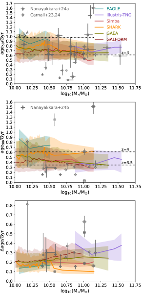
Figure 9: Top panel: Lookback time to when the $z=3$ massive-quenched galaxies had formed $50$% of their stellar mass as a function of the $z=3$ stellar mass, for all the simulations, as labelled. Lines with shaded regions show the medians and the $16^{\rm th}-84^{\rm th}$ percentile ranges, respectively. We use adaptive bins to ensure a number of galaxies per bin $\geq 10$. For reference, the horizontal dotted lines show $z=4$ and $z=5$. Here we also show observationally-derived measurements of $\rm age_{\rm 50}$ from Nanayakkara et al. (2024) and in preparation and Carnall et al. (2023a, 2024) as open symbols, as labelled. Middle panel: As in the top panel but for when the galaxies had formed $90$% of their stellar mass. The horizontal dotted lines show $z=3.5$ and $z=4$. Here we show observations from Nanayakkara et al. (in preparation) and Carnall et al. (2024) (which is the subsample of the top panel that is spectroscopically confirmed). Although we have $\chi^{2}$ errors associated with the inferred SFHs for the observations, those represent lower limits, so we apply a $10$% error to all measurements, acknowledging that the real uncertainties are likely larger. Bottom panel: as in the middle panel but for the time it took for the galaxies to go from $50$% to $90$% of their $z=3$ stellar mass.

To quantify this better, we show in the top and middle panels of Fig. 9 the relationship between $\rm age_{\rm 50}$ and $\rm age_{\rm 90}$, respectively, with stellar mass (see § 2.3 for the definitions of these properties). Eagle tends to produce the oldest massive-quenched galaxies, while those in Simba and Galform are the youngest (though some dependence on stellar mass emerges). The latter is especially clear with $\rm age_{\rm 90}$. Illustris-TNG and GAEA predicts ages that are similar or slightly older than Simba and Galform, while Shark predicts ages that are between those of Eagle and the rest of the simulations. Massive-quenched galaxies in Eagle have formed $90$% of their stars by $z\approx 4-4.5$, making them very old compared to the other simulations. Note that none of the simulations predict a well established age-mass relation within this population.

The top panel of Fig. 9 shows observationally-derived $\rm age_{\rm 50}$ from Carnall et al. (2023a, 2024); Nanayakkara et al. (2024). For Carnall et al. (2023a) we find that adding or not the non-robust quenched galaxies makes little difference to the median and standard deviation presented with the filled diamond. In the middle and bottom panels we show observations from Nanayakkara et al. (in preparation) and Carnall et al. (2024). The latter are the sub-sample of galaxies in the top panel that are spectroscopically confirmed. The available data is currently too scarce leading to a large scatter, which makes it consistent with all the simulations within the errorbars. Increasing the sample sizes may help disentangle the predictions presented here.

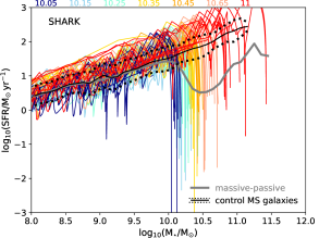
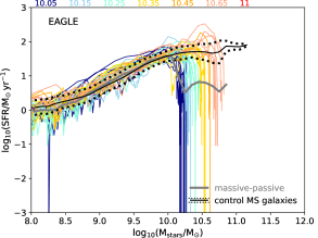
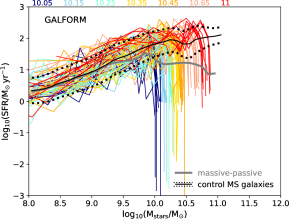
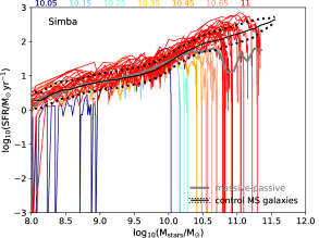
Figure 10: The evolution of the $z=3$ massive-quenched galaxies shown in Fig. 6 in the SFR-stellar mass plane in each simulation, as labelled. Lines are coloured depending on their $z=3$ stellar mass using the same bins of Fig. 6. The median SFR in bins of stellar mass of all the $z=3$ massive-quenched galaxies is shown with a thick-grey line in each panel. For comparison, in each panel we also plot the median and one standard deviation of the control MS sample (defined in § 2.3) with solid and dotted black lines, respectively.

Several recent papers have used the difference between e.g. $\Delta\,\rm age=\rm age_{\rm 90}-age_{\rm 50}$ to quantify a formation timescale (e.g. de Graaff et al. 2024). We show this in the bottom panel of Fig. 9. From this difference we see that Illustris-TNG galaxies are the ones that form the slowest, while Eagle and Shark galaxies form the fastest. Simba, GAEA and Galform produce $\Delta\,{\rm age}$ that are in between the other simulations. The difference is quite large, with Illustris-TNG taking a factor of $\approx 3$ ($\approx 1.7$) times longer to form compared with Shark (Simba) galaxies of the same stellar mass. Note that the Illustris-TNG’s timescales are similar to those reported by Weller et al. (2024) for the same simulation using slightly different definitions. Kimmig et al. (2023) found that in Magneticum (a cosmological hydrodynamical simulation), massive-quenched galaxies have $\Delta\,\rm age\lesssim 170$ Myr, similar to what we find in Shark and Eagle. In observations, inferred $\Delta\,\rm age$ are mostly between $100-300$ Myr (e.g. see symbols in the figure), closer to what Shark, Eagle, Simba, Galform and GAEA predict, but the scatter is again too large to reach a robust conclusion.

4.2.2 The growth of galaxies in the SFR-stellar mass plane

To understand what drives the diversity of ages and $\Delta\,\rm age$, we turn our attention to the way galaxies grow in the SFR-stellar mass plane in Fig. 10. Most galaxies in Shark, Eagle and Simba show periods in their SFH where galaxies are clearly above main sequence (by more than $\gtrsim 0.3$ dex), in the starburst region. When not in the starburst region, galaxies grow along the main sequence. The latter is seen by the similarity between the median SFR-stellar mass relation of the massive-quenched and control MS samples before quenching happens in the former sample. In Galform clear starbursts episodes are seen when galaxies are still relatively low mass $M_{\star}\lesssim 10^{9.5}\,\rm M_{\odot}$, while at higher mass galaxies mostly grow along the main sequence.

Galaxies in Illustris-TNG grow along a very tight SFR-stellar mass sequence that is slightly elevated compared with the main sequence, but showing little deviations to higher SFRs. In GAEA we see that massive-quenched galaxies grow along the main sequence for most of their lives until quenching. In the latter, quenching is very sudden and generally happens in a single simulation snapshot. The fact that galaxies in GAEA and Illustris-TNG show almost no starburst episodes and that in Galform they show clear starbursts only very early on their formation history, is why they take the longest to form (see bottom panel in Fig. 9). Despite these differences, we find that in all simulations galaxies spend most of their time on the main sequence (between $55-99$% of their active lives, with the extremes of the range corresponding to Galform and GAEA respectively). The large difference between the fraction of time galaxies spend on the main sequence between Galform and GAEA is due to the inclusion of disk instability-driven starbursts in the former and the lack of thereof in the latter. This is clear from studying the contribution of disk instabilities to the SFRs of galaxies across cosmic time in Galform (see discussion in § 5.3 in Lacey et al. 2016). Shark also includes disk instability-driven starbursts and predicts galaxies spend $73$% of their lives on the main sequence, again much less than what is found in GAEA. Despite spending most of their lives on the main sequence, at their peak SFR, galaxies in most simulations are above the main sequence as shown in Fig. 7.

Fig. 10 also shows that in Shark, Eagle, Simba, Galform and GAEA there is a small fraction of $z=3$ massive-quenched galaxies that have had periods of passiveness in the past. These periods of passiveness are perhaps reminiscent of what has been called “min-quenching” in the literature (Looser et al., 2023), albeit at slightly higher stellar masses, where galaxies are likely to rejuvenate after such passive periods. The galaxies here, indeed go back to the main sequence or even the starburst region after those “mini-quenching” periods. Such periods are seen in the SFHs of some $z=3$ massive-quenched galaxies in all the simulations, except for Illustris-TNG. The latter is related to lack of massive-quenched galaxies in Illustris-TNG at $z\gtrsim 3.5$ shown in Fig. 3. We will go back to this in § 4.3.

Another interesting difference between the simulations is the tightness of the main sequence, with Galform predicting the least tight sequence (with a typical standard deviation of $\approx 0.45$ dex) and Illustris-TNG, the tightest one (standard deviation of $\approx 0.14$ dex). Shark, Eagle, Simba and GAEA predict a main sequence standard deviation of $\approx 0.3$, $\approx 0.2$, $\approx 0.25$, and $\approx 0.2$ dex, respectively. Spectroscopic observations with the JWST are starting to place constraints on the intrinsic scatter of the main sequence. Clarke et al. (2024) found values of $0.4-0.5$ dex at $z\gtrsim 3$ for galaxies with stellar masses $\lesssim 10^{10}\,\rm M_{\odot}$, similar to what Galform predicts and larger than the other simulations’ predictions. One caveat is that samples are still very small (Clarke et al. 2024 employed 104 galaxies to measure the main sequence’s scatter in $5$ redshift bins), and hence bigger samples are required to get more robust measurements (see D’Silva et al. 2023a).

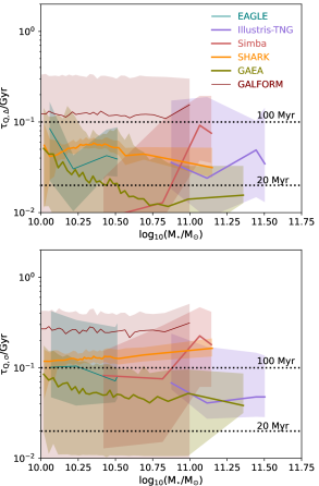
Figure 11: Top panel: quenching timescale, $\tau_{\rm Q,\Delta}$ (defined in terms of $\Delta_{\rm MS}$; see § 2.3) as a function of the $z=3$ stellar mass of massive-quenched galaxies in each of the $6$ simulations, as labelled. Lines with shaded regions are as in Fig. 7. Bottom panel: as in the top panel but for $\tau_{\rm Q,\sigma}$ (defined in terms of $\Delta_{\rm MS}/\sigma_{\rm MS}$; see § 2.3).

4.2.3 Quenching timescales of $z=3$ massive-quenched galaxies

Finally, we study in Fig. 11 the quenching timescales of the massive-quenched galaxies in each simulation. We use the two definitions introduced in § 2.3. When we measure the quenching timescale in terms of distance to the main sequence only ($\tau_{\rm Q,\Delta}$), we see that the quenching of the most massive-quenched galaxies happens very fast in all the simulations ($\tau_{\rm Q,\Delta}\lesssim 100$ Myr), except in Galform which has a median of $\tau_{\rm Q,\Delta}\approx 150$ Myr, and a significant population that scatters up to $\tau_{\rm Q,\Delta}\approx 300$ Myr.

However, when we take into consideration the tightness of the main sequence in each simulation and measure quenching in terms of $\sigma$ deviations from the main sequence (bottom panel of Fig. 11), we see that galaxies in all simulations tend to take longer: in Shark, eagle and Simba galaxies quench in $\approx 100-200$ Myr, while Galform’s galaxies tend to take on average $\approx 300$ Myr to quench. The quenching timescales in Illustris-TNG and GAEA continue to be below $100$ Myr. We note, however, that such quenching timescales are much smaller than the time step of MILL, employed in GAEA, and hence we can only assert that they are smaller or similar to $100$ Myr.

The interpretation of quenching timescales one can draw from Fig. 11 and the bottom panel of Fig. 9 can be very different in some models (see for example the change in Simba between the top and bottom panels of Fig. 11), which emphasises the need for a convergent definition of quenching timescale in the literature.

4.3 How AGN feedback shapes the SFHs of early massive-quenched galaxies

Below we connect the results of previous sections with how AGN feedback is implemented in each simulation.

In Illustris-TNG, AGN feedback in the radiatively-efficient mode has very little impact on the capability of galaxies to be star-forming (Kurinchi-Vendhan et al., 2023). Hence, galaxies appear to grow along a tight sequence in the SFR-stellar mass plane until a milestone is reached and they are quickly quenched, in $<100\,\rm Myr$. At $z=0$, that milestone is the BH reaching a mass of $10^{8.2}\,\rm M_{\odot}$, when kinetic feedback kicks in (Terrazas et al., 2020). The BH transition mass that quenches galaxies is clearly seen in Fig. 12, where we see that Illustris-TNG predicts a clear transition around the mass highlighted with a vertical line; galaxies below that mass are star-forming, and above are passive. The transition is extremely sharp in Illustris-TNG. This happens at around $10^{8.6}\,\rm M_{\odot}$ at $z=3$, which is higher than the $z=0$ transition mass of $10^{8.2}\,\rm M_{\odot}$ due to the overall accretion rates onto BHs being higher at higher redshifts in the absence of AGN feedback. GAEA also displays a form of BH mass transition at $10^{7}\,\rm M_{\odot}$, with galaxies preferentially deviating from the main sequence above that mass. Note, however, that this transition is not sharp as it is in Illustris-TNG, and the scatter around the median can be as high as $\approx 2$ dex.

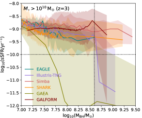
Figure 12: The sSFR as a function of the central BH mass for all galaxies at $z=3$ that have a stellar mass $>10^{10}\,\rm M_{\odot}$, in all the simulations, as labelled. Lines with shaded regions show the medians and $16^{\rm th}-84^{\rm th}$ percentile ranges, respectively. We use adaptive bins to ensure a number of galaxies per bin $\geq 10$. The horizontal dotted line shows our passive sSFR criterion, while the vertical dotted line shows the approximate BH mass at which galaxies in Illustris-TNG go from being star-forming to passive.

For the other simulations, Shark, Eagle, Simba and Galform we see a similar behaviour, where massive BHs ($\gtrsim 10^{8}\,\rm M_{\odot}$) are associated with the $16^{\rm th}$ percentile being close or dropping below the sSFR threshold used to classify galaxies as passive. However, the medians remain comfortably above the sSFR threshold. The lack of a clear BH mass threshold marking the transition from star-forming to passive in most of the simulation in Fig. 12 is simply a reflection of other properties besides the BH mass being important in determining when and how AGN feedback is effective in quenching galaxies.

Going back to Illustris-TNG, we find that the sudden effect of kinetic feedback and the lack of effective feedback below a BH mass threshold is the reason why there are almost no quenched galaxies at $z\gtrsim 3.5$ (Fig. 3), and why there are virtually no $z=3$ quenched galaxies with stellar masses $10^{10}\,\rm M_{\odot}\lesssim M_{\star}\lesssim 10^{11}\,\rm M_{\odot}$ in this simulation (Fig. 4). The lack of effective feedback before galaxies hit a certain BH mass is also the reason why this simulation predicts massive-quenched galaxies to have higher stellar masses than the other simulations (see Fig. 4), and a baryon collapse efficiency that is higher compared to most of the other simulations (Fig. 5)

Simba’s AGN feedback model has several similarities to the one implemented in Illustris-TNG as pointed out by Davé et al. (2019) (e.g. two modes of AGN feedback, with the kinetic+thermal modes acting on slowly accreting BHs being what is effective in quenching galaxies; and a BH mass threshold above which the latter feedback can act). Hence, it is not surprising that there are some similarities in the AGN feedback impact: Simba struggles to produce the density of intermediate-mass passive galaxies, and produces a similarly high baryon collapse efficiency. However, there are also several differences, with massive-quenched galaxies having progenitors that oscillate a lot more around the main sequence as they grow compared with Illustris-TNG (Fig. 10). Another important condition for AGN feedback to be effective in Simba besides the BH mass, is the Eddington ratio, which is required to be $<0.2$ for the jet mode to be effective, with the peak efficiency happening at an Eddington ratio of $0.02$. At high redshift this rarely happens (Thomas et al., 2021), leading to an overall small fraction of massive-quenched galaxies (see Table 1. This emphasises the condition of galaxies to be massive before they can undergo effective AGN feedback quenching. Hence, because the BH mass is not the only important parameter determining the regimes in which AGN feedback is effective, Simba does not produce a strong correlation between sSFR and BH mass (Fig.12).

Shark’s AGN feedback model acts in a way that galaxies can get affected and fall significantly below the main sequence, but then regrow and go back to it. This can naturally happen as a jet power is always computed and can potentially produce feedback as long as there is a hot halo to work against. As soon as the BH does not produce enough jet power, then quenching becomes less efficient and BHs can go out of the maintenance mode. Hence, there is a natural stochasticity associated with the model. Lagos et al. (2024) mention that even though Shark includes a model for AGN wind-driven feedback, in general this has a small effect compared to the jet feedback model. Because AGN feedback in general can be effective early in the formation of galaxies in Shark, galaxies then struggle to get to extremely high masses, $\gtrsim 10^{11}\,\rm M_{\odot}$, by $z=3$ and the model ends up predicting too few extremely massive galaxies.

Eagle’s AGN feedback model becomes efficient as soon as the outflows driven by stellar feedback cease to be buoyant (and hence become less effective). The latter happens at around a halo mass of $10^{12}\,\rm M_{\odot}$ (Bower et al., 2017). This was not modelled explicitly but instead is a consequence of how stellar and AGN feedback interact. AGN feedback thus can be effective quite early on in a galaxy’s history, preventing them from growing too much in stellar mass. Similarly to Shark, this thus leads to the lack of extremely massive galaxies at early cosmic times.

Galform employs a model of AGN feedback that depends on the formation of a hot halo and the Eddington luminosity of BHs (rather than its accretion rate, which is directly or indirectly what the other simulations use). The only way this AGN feedback model acts is by stopping gas cooling, and hence the quenching necessarily happens on a scale similar to the star formation efficiency (i.e. what depletes the remaining gas reservoir in galaxies). This is a slow process and hence why Galform tends to produce the longest quenching timescales of all simulations (Fig. 11).

GAEA’s latest AGN feedback implementation seems to be particularly effective at very high stellar masses. They quench extremely quickly going passive within a single snapshot of the simulation and as soon as galaxies reach modest BH masses (see Fig. 12). Because the AGN quasar wind scales with the AGN bolometric luminosity without an explicit dependence on the available gas reservoir, it makes quenching very strongly dependent on BH mass and weakly on other galaxy properties. This leads to a strong correlation between sSFR and BH mass, which is not seen in the other simulations.

Interestingly, in GAEA most of the quenching of massive-quenched galaxies is due to quasar winds as detailed in De Lucia et al. (2024). They show this by switching off that model and finding very few quenched galaxies at high redshift. In Shark and Galform instead, quenching happens when a form of mechanical feedback is implemented (similar to what is done in Simba and Illustris-TNG). The Eagle AGN feedback model, even though it injects the energy in a thermal mode, the way it quenches galaxies ends up being phenomenologically similar to the classical “radio-mode” feedback (Croton et al., 2006); see Bower et al. (2017) for details. This is because the quenching is not associated with gas being ejected from the galaxy but with heating a galaxy’s corona and preventing further cooling. We remark, however, that sometimes in hydrodynamical simulations it is hard to fully disentangle the role of ejective vs preventative AGN feedback (Brennan et al., 2018).

Figure 13: The central BH mass a function of stellar mass for all galaxies at $z=3$ that have a stellar mass $>10^{10}\,\rm M_{\odot}$, in all the simulations as labelled (dotted lines). We also show separately passive ($\rm sSFR<10^{-10}\,\rm yr^{-1}$) and active ($\rm sSFR>10^{-10}\,\rm yr^{-1}$) galaxies, with solid and dashed lines, respectively. Lines show the medians, and the shaded regions (shown only for the passive and active sub-populations) the $16^{\rm th}-84^{\rm th}$ percentile ranges, respectively. We use adaptive bins to ensure. a number of galaxies per bin $\geq 10$. We also show with symbols observational inferences from Decarli et al. (2010a, b) (D+10), Suh et al. (2020) (S+20) and Poitevineau et al. (2023) (P23), as labelled in the top-right panel, corresponding to measurements at $2\leq z\leq 3.7$.

Fig. 13 shows the BH-stellar mass relation for massive galaxies in all the simulations, separating active ($\rm sSFR>10^{-10}\,\rm yr^{-1}$) and passive ($\rm sSFR\leq 10^{-10}\,\rm yr^{-1}$) galaxies. Shark, Eagle, Illustris-TNG, Simba and GAEA predict a clear difference between active and passive galaxies, with passive galaxies having more massive BHs at fixed stellar mass than their active counterparts. The quantitative difference however, varies widely between the simulations: Shark, Eagle, Illustris-TNG, Simba and GAEA produce differences of $\approx 0.25$, $0.4$, $0.3-0.75$, $0.1-0.5$ and $\gtrsim 1.5$ dex, respectively, between the two populations. At $z=0$, there is a documented difference between passive and star-forming galaxies (Terrazas et al., 2017), where the former have more massive BHs than the latter at fixed stellar mass. Lagos et al. (2024) showed that at $z=0$ and in Shark the difference can be as high as one order of magnitude, in agreement with what Terrazas et al. (2017) find. At these high-z however, the samples are too small still to split between star-forming and passive galaxies, but this is likely to improve, with high-precision JWST BH-mass measurements using reverberation mapping becoming available (Golubchik et al., 2024). Hundreds of such measurements are expected to be carried out with Euclid (Euclid Collaboration et al., 2024) in the near future and thousands with the Roman space telescope in the longer term.

The explicit BH-mass dependence of the switch to go from the radiatively efficient to inefficient modes of AGN feedback in Simba and Illustris-TNG lead to a difference in BH mass between the passive and star-forming population that increases with decreasing stellar mass. This is not seen in the other simulations, where there is either only a single mode of AGN feedback (eagle and Galform), or where the transition between modes does not depend on BH mass (Shark and GAEA).

Kimmig et al. (2023) and Weller et al. (2024) show that a similar BH mass difference is seen in the Magneticum and Astrid simulations, respectively. Conversely, Galform predicts no difference between the BH masses of active and passive galaxies at fixed stellar mass. The simulations in which a clear difference in BH mass is seen have AGN feedback models that depend strongly on the BH accretion rate while in Galform, the most important condition is that the halos are in quasi-hydrostatic equilibrium. The latter thus leads to little BH mass differences between massive and passive galaxies. It is, however, fair to say that the vast majority of simulations (including those analysed here) predict passive galaxies to have more massive BHs than active counterparts.

On the other extreme, in GAEA, star-forming galaxies seem to prefer very low BH masses, that deviate by orders of magnitude from the local BH-stellar mass relation, and more so considering the latest JWST results, which tend to prefer a higher normalisation at $z=3$ (e.g. Bertemes et al. 2024; Furtak et al. 2024). Current observational estimates are shown as symbols, and tend to prefer higher masses, implying that GAEA’s predictions may be in tension with observations unless they are biased towards passive galaxies. Note, however, that within the scatter, most of the simulations agree with the observational constraints quite well.

Regarding the stellar populations of massive-quenched galaxies, Kimmig et al. (2023) show that the short formation timescales predicted for massive-quenched galaxies at high-z in Magneticum ($\Delta\,\rm age\lesssim 200$ Myr) leave clear imprints in the form of e.g. alpha-enhancements, flat age gradients and steep metallicity profiles. Similar features would be expected for the simulations here that predict similarly short formation timescales (e.g. Eagle and Shark; see bottom panel of Fig. 9).

The impact of the different AGN feedback models implemented in the simulations is also seen in the gaseous halos around galaxies (Wright et al., 2024) even at $z=2$ (with many of the differences becoming larger towards $z=0$). For example, Wright et al. (2024) show that the gas content and gas temperature of halos in Eagle, Illustris-TNG and Simba can differ by $30$% and $1.5$ dex, respectively, at the scales where AGN feedback is effective. However, observing the gaseous halos of high-z galaxies is challenging, and hence it is promising to see that AGN feedback also impacts galaxy properties of massive-quenched galaxies that can perhaps be more easily collected.

Every simulation thus have a different implementation of AGN feedback, which has a clear impact on how galaxies grow and end up quenching, including how quickly that happens. This impact is clearly seen in the SFHs of massive-quenched galaxies at $z=3$. This is not to say that other baryon physics processes do not affect the way in which massive galaxies grow in these simulations, but simply that AGN feedback is required to produce the quenching. As the observational samples grow in size, studying the differences in SFHs of passive galaxies in bins of stellar mass would greatly help disentangle some of the predictions presented in this paper.

5 Conclusions

We have presented a thorough study of the SFHs of high-z massive-quenched galaxies in $6$ modern galaxy formation simulations ($3$ SAMs, Shark, GAEA, Galform; and $3$ cosmological hydrodynamical simulations, Eagle, Illustris-TNG, Simba). All of these have been primarily tuned to the local Universe (except for GAEA), so the comparisons performed in this paper constitute real tests of the predictions of these simulations.

We summarise our main findings below:

• All the simulations struggle to easily reproduce the number density of massive-quenched galaxies observed by the JWST (e.g. Carnall et al. 2023a; Valentino et al. 2023; Nanayakkara et al. 2024; Alberts et al. 2023), especially at $z\gtrsim 3$. However, there are varying degrees of tension (from $\approx 0.3$ dex to several dex) depending on the exact stellar mass and sSFR used to select the samples in simulations (Fig. 3).

• Comparing the simulations with observations of the $z\approx 3$ stellar mass function of passive galaxies reveals that there are broadly two distinct behaviour outcomes: Simba and Illustris-TNG reproduce relatively well the number density of passive galaxies with $M_{\star}\gtrsim 10^{11}\,\rm M_{\odot}$ but fall short at $10^{10}\lesssim M_{\star}\lesssim 10^{11}\,\rm M_{\odot}$. The opposite is true for Shark, Galform, Eagle and GAEA (Fig. 4). We find that this is due to the explicit dependence on the BH mass of the switch to go from the radiatively-efficient to inefficient AGN feedback modes in Simba and Illustris-TNG, which allows galaxies to grow efficiently until their BHs hit a certain mass. In Simba this is compounded with the slow build-up of the jet mode efficiency, which reaches its peak at a very low Eddington ratio of $0.02$. A consequence of this difference between Illustris-TNG, Simba and the rest of the simulations is the higher baryon collapse efficiency at fixed halo mass, $\approx 15-30$%, in the former simulations (Fig. 5).

• The SFHs of the $z=3$ massive-quenched galaxies present several differences between the simulations. Shark, Eagle and Illustris-TNG predict their formation to start at $z\gtrsim 10$ (i.e. appear for the first time in the catalogues), while in Galform, Simba and GAEA a large fraction of the star-forming progenitors start forming at $z<10$ (Fig. 6). The peak SFRs of the galaxies in every case depend strongly on the $z=3$ stellar mass but with Shark and Galform predicting peak SFRs $\approx 0.5-0.7$ dex higher at fixed stellar mass than the other simulations due to the higher star formation efficiency they invoke for starbursts (Fig. 7). However, relative to the main sequence, we find that Shark, Galform, Illustris-TNG and Simba predict galaxies to be starbursting at their peak SFR (i.e. well above the main sequence), while this is only true for the most massive galaxies in eagle and GAEA.

• Compared with observationally-inferred SFHs, we find that Shark and Illustris-TNG produce the highest SFR peaks, closer to the observations (Fig. 8). However, the observational samples are very small and the inferences sensitive to the exact details of the spectral modelling and the spectral resolution of the available data. We also compare the simulations with the formation times derived in the literature for massive-quenched galaxies (defined as the time where half of the stellar mass has been formed) and find that within the scatter ($\approx 300-1,000$ Myr), all the simulations agree well with observations (Fig. 9).

• Shark and Eagle produce the earliest and fastest-forming galaxies, while Galform and Illustris-TNG predict the latest and slowest-forming galaxies (Fig. 9). Shark, Eagle and Simba predict $\Delta\,\rm age\lesssim 200$ Myr (with $\Delta\,\rm age$ being the difference between the time at which galaxies reach $50$% and $90$% of their $z=3$ stellar mass), while the other simulations prefer $\Delta\,\rm age\gtrsim 200$ Myr, with $\Delta\rm age$ being the difference between the time the $z=3$ massive-quenched galaxies had formed $50\%$ and $90$% of their stellar mass. By measuring the quenching timescale in terms of distance to the main sequence (which we define internally to each simulation for consistency) we find that all the simulations, except for Galform, predict quenching timescales $\lesssim 100$ Myr (Fig. 11). However, if we consider the tightness of the main sequence, we see that the timescales for quenching become longer in a way that in eagle, Shark, and Simba they are $\approx 100-200$ Myr, emphasising the need for a convergent definition of quenching timescale.

• By comparing the sSFR with the BH mass of galaxies at $z=3$ with $M_{\star}>10^{10}\,\rm M_{\odot}$, we find that only Illustris-TNG and GAEA produce a strong correlation between the two (Fig. 12). In Illustris-TNG this looks like a sharp transition from star-forming to quenched galaxies at a BH mass of $\approx 10^{8.65}\,\rm M_{\odot}$. In GAEA, galaxies start quenching as soon as they reach a relatively modest BH mass of $10^{7}\,\rm M_{\odot}$, so that the BH-stellar mass relation of star-forming galaxies is $\approx 1.5$ dex lower in normalisation compared with passive galaxies (Fig. 13).

• All the simulations, except for Galform, predict passive galaxies to have heavier BHs than their star-forming counterparts at fixed stellar mass (Fig. 13). The lack of difference in Galform is due to AGN feedback primarily depending on whether a halo is found to be on quasi-hydrostatic equilibrium, which is independent of BH mass.

Our findings combined with literature ones (Vani et al., 2024; Weller et al., 2024; Szpila et al., 2024) point to the pervasive problem of reproducing the properties of massive-quenched galaxies in the early universe in modern cosmological galaxy formation simulations. The amount of tension with current observations is extremely sensitive to potential errors in stellar masses and SFRs, and contamination of the passive galaxy samples in observations. Significant effort is required to understand the magnitude of errors in the derivation of these quantities in observations to have a precise understanding of the true tension with the simulations.

We also find that the exact way AGN feedback is modelled leaves clear imprints on the SFHs of massive-quenched galaxies in a way that there are clear differences in the predictions of the different simulations presented here that are testable with existing facilities and upcoming observations. In fact, recent observations are beginning to place constraints on the SFHs of massive-quenched galaxies across different cosmic epochs offering a unique and novel opportunity for further testing of the models using observations.

Data Availability

The data for each simulation is available as follows:

• Shark: The surfs halo and subhalo catalogue and corresponding merger trees used in this work can be accessed from https://tinyurl.com/y6ql46d4. Shark is a public code and the source and python scripts used to produce the plots in this paper can be found at https://github.com/ICRAR/shark/.

• Galform: the data used in this paper is publicly available from http://virgodb.dur.ac.uk:8080/MyMillennium/.

• GAEA: data and code are proprietary and access can be given upon request. Visit https://sites.google.com/inaf.it/gaea/home for details.

• Eagle: The Eagle simulations are publicly available; see McAlpine et al. (2015); The EAGLE team (2017) for how to access EAGLE data.

• Illustris-TNG: data is publicly available from https://www.tng-project.org (Nelson et al., 2019).

• Simba: data is publicly available from http://simba.roe.ac.uk/.

Appendix A The main sequence evolution and control samples

§ 2.3 presents the way we construct a control sample of massive-active galaxies in each simulation, and explains how we use that control sample to measure a distance to the main sequence and define quenching timescales. Here, we show that this is a good assumption by comparing the median SFR-stellar mass relation of the control sample presented in Fig. 10 (solid and dotted black lines) with the main sequence across different redshifts in each simulation. This is presented in Fig. 14.

Each panel of Fig. 14 shows the median SFR in bins of stellar mass at $z=9,\,7,\,5,\,4$ using colour lines, with the coloured shaded regions showing $1$ standard deviation around the median. The latter is measured using the galaxy catalogues produced at each of these snapshots using the same SFR and stellar mass definitions introduced in § 2.3.

Each panel of Fig. 14 also shows, using black lines, the median and $1\sigma$ dispersion of the SFR-stellar mass tracks of the control MS sample. The latter is also coloured by the median redshift of the points in the tracks in bins of stellar mass (with the grey-colour band at the top showing the corresponding median redshifts). Typically the lower mass part of the SFR-stellar mass tracks of the control MS sample, $M_{\star}\lesssim 10^{8.7}\,\rm M_{\odot}$ are dominated by the early growth of those galaxies, with typical median redshifts of $9$ or $8$. The control MS sample galaxies typically reach a stellar mass of $M_{\star}\approx 10^{9.5}\,\rm M_{\odot}$ by $z\approx 5$. The exact redshifts at which this happens varies slightly between simulations.

We see that the main sequence traced by the SFR-stellar mass tracks of the control MS sample is flatter than the main sequence measured at individual redshifts in all the simulations. This is because different parts of the main sequence traced by the SFR-stellar mass tracks of the control MS sample correspond to different redshifts. The lower mass part tends to follow well the main sequence measured at $z=9$ while the higher mass parts are better described by the main sequence at $z=5$ or $z=4$. In principle, we could measure a distance to the main sequence at each point in the evolution of the massive-passive galaxy sample of each simulation using a main sequence defined at the same redshift of the point of interest (which is the more common approach adopted in the literature). However, the cadence of the snapshot outputs of the simulations is not as good as the cadence we use to reconstruct the SFHs of the massive-passive galaxies. To circumvent this issue, we define an alternative main sequence using the SFR-stellar mass tracks of the control MS sample, which in turns gives us a time dependent main sequence (due to the median redshift changing along the main sequence of the control MS sample). The fact that the median redshift of the different stellar mass portions of the control MS sample follow the measured main sequence at a redshift close to the median one implies that using the control MS sample to measure distance to main sequence would give a similar result to using the main sequence defined at individual redshifts. This means that the control MS sample is, on average, growing along the main sequence.

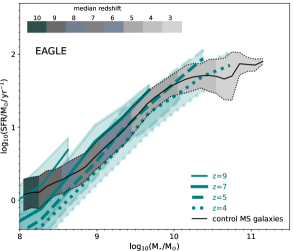
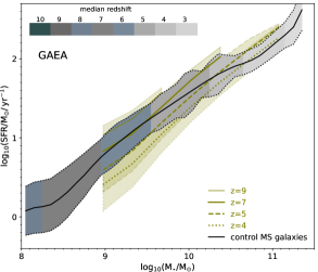
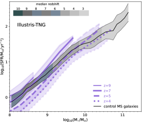
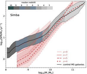
Figure 14: The median relation between SFR and stellar mass with $1\,\sigma$ (standard deviation) of the control MS sample (solid and dotted lines, respectively) compared with the main sequence predicted in each simulation at $z\approx 9,\,7,\,5,\,4$ (as labelled in each panel). We colour the control MS sample by the median redshift of the data points in bins of stellar mass, as labelled in each panel. This is shown for the $6$ simulations Shark  Eagle, GAEA, Illustris-TNG, Galform and Simba, as labelled in each panel. Note that for GAEA we only use galaxies with stellar masses $\geq 10^{9}\,\rm M_{\odot}$, while for the other simulations we cover the entire stellar mass range.

Appendix B Number density of massive-quenched galaxies in the Magneticum simulations

One of the only cosmological hydrodynamical simulations to agree better with current observations of the number density of massive-quenched galaxies at $z=3-4$ is Magneticum (Remus & Kimmig, 2023; Kimmig et al., 2023). Here we show the number density of galaxies in Magneticum with $M_{\star}\geq 10^{10}\,\rm M_{\odot}$ and $\rm sSFR\leq 10^{-10}\,\rm yr^{-1}$ in Fig. 15.

Figure 15: As in Fig. 3 but for the Magneticum simulations and using a single selection for massive-quenched galaxies: $M_{\star}\geq 10^{10}\,\rm M_{\odot}$ and $\rm sSFR\leq 10^{-10}\,\rm yr^{-1}$.

Magneticum indeed produces a higher number density of massive-quenched galaxies at $z=3-4$ compared with the simulations presented in Fig. 3. However, it tends to overpredict by an order of magnitude the number of massive-quenched galaxies at slightly lower redshift, $z=2-3$. Lustig et al. (2023) showed that at $z=2$ Magneticum produced roughly the correct number density of masses $\geq 10^{11}\,\rm M_{\odot}$, indicating that the problem is that Magneticum is producing too many passive galaxies with masses $10^{10}-10^{11}\,\rm M_{\odot}$.

This over-production of intermediate-mass quenched galaxies could be in part due the AGN feedback model been overly effective in Magneticum, and in part due to resolution. The resolution of the box used here (DM and gas particle masses of $5.1\times 10^{7}\,\rm M_{\odot}$ and $1.03\times 10^{7}\,\rm M_{\odot}$, respectively), which is the same as used in Remus & Kimmig (2023); Kimmig et al. (2023), is $10$ times worse than that used in EAGLE and Illustris-TNG, which could lead to overly effective quenching at around a stellar mass of $10^{10}\,\rm M_{\odot}$ and below. Regardless of the exact causes, this shows that in the models analysed in this work and others, such as Magneticum, the agreement with observations of massive-quenched galaxies in one redshift does not warrant the agreement over a wide redshift range.

Appendix C The effect of the time cadence on the maximum SFR

Fig. 16 shows the equivalent to the top-left panel of Fig. 7 but when we sample the SFHs in Shark, Eagle, Illustris-TNG and Simba to have timesteps that are $\approx 180$ Myr, to make them more comparable to the time cadence of GAEA and Galform. We see small changes - for example $\rm SFR_{\rm max}$ in GAEA is similar to that of Simba, while Illustris-TNG has the smallest values; at stellar masses $\lesssim 10^{10.5}\,\rm M_{\odot}$ Galform produces higher $\rm SFR_{\rm max}$ than Shark, but this reverts at higher stellar masses. However, qualitatively the results and hence our conclusions remain.

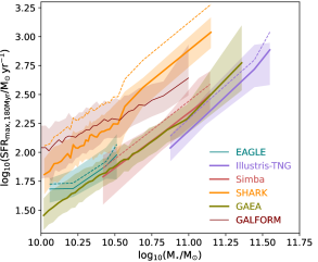
Figure 16: $\rm SFR_{\rm max}$ as a function of the $z=3$ stellar mass of massive-quenched galaxies in $6$ simulations, as labelled. The solid lines and shaded regions show the medians and $16^{\rm th}-84^{\rm th}$ percentile ranges, respectively. We sample the SFHs of galaxies in Shark, Eagle, Illustris-TNG and Simba using a poorer time cadence that resembles that of GAEA and Galform ($\approx 180$Myr). To facilitate the comparison with Fig. 7, we show with dashed lines the medians presented there for Shark, Eagle, Illustris-TNG and Simba, with are the simulations whose SFHs are being resampled. Overall we see similar results to those presented in the top-left panel of Fig. 7: Shark and Galform produce the highest $\rm SFR_{\rm max}$, while Illustris-TNG produces the lowest values.

Appendix D Fits to the star formation histories

We fit each SFH with a skewed Gaussian function (as presented in Robotham et al. 2020):

$$X{\rm(age)} = \frac{{\rm age}-m_{\rm peak}}{m_{\rm period}},$$ (1)

$$Y{\rm(age)} = X{\rm(age)}*\left(e^{m_{\rm skew}}\right)^{\rm asinh({\it X}{\rm(age)})}$$ (2)

$${\rm SFR(age)} = m_{\rm SFR}\,e^{-Y^{2}{\rm(age)}/2},$$

where “age” is the lookback time from the redshift of interest, and $m_{\rm peak}$, $m_{\rm period}$, $m_{\rm SFR}$ and $m_{\rm skew}$ are parameters. We choose this function because its parameters are orthogonal and that makes it better from a statistical point of view than a function in which the parameters are potentially are degenerate with each other. It has also been used to fit galaxies at high-z in D’Silva et al. (2023b, c). We acknowledge however, that other functions have more broadly been used to fit the SFHs of high-z galaxies than the one used here (e.g. Schreiber et al. 2018; Carnall et al. 2020).

We employ Highlander to fit the above function to each SFH, which uses a combination of genetic algorithms and Markov Chain Monte Carlo (MCMC), thus, providing a global minimum and likelihood. With the best fit, we compute a “goodness” function:

$${\rm goodness}={\rm log}_{10}\left(\frac{\Sigma_{i}|\rm data-model|}{\,N_{\rm d.o.f.}\,\,M^{f}_{\star}}\right),$$ (4)

where $N_{\rm d.o.f.}$ is the number of degrees of freedom (in this case the number of timesteps with which the SFH is sampled), and $M^{f}_{\star}$ is the total stellar mass a galaxy has formed (which is different to the actual galaxy stellar mass at $z=3$ due to stellar evolution). Note that the normalisation is required to compare between galaxies, and the quantity is logged to avoid large numbers. We use this measure to isolate galaxy candidates that have had multiple starburst episodes. We find that internally to each simulation, ${\rm goodness}$ is a good parameter to isolate those galaxies, even though the exact threshold marking the transition from uni-modal distributions to multiple peaks changes between each simulation. We find that a threshold value between $-9.9$ and $-9.6$ work for all the simulations, and we tune the exact threshold to each simulation (values are included in the captions of Figs. 17, 18, 19, 20, 21, and 22).

Note that here we are interested in multiple starburst episodes that are unrelated with each other. As an example, in Shark (Fig. 20), there are galaxies going through multiple starbursts episodes but that appear correlated (i.e. a galaxy is having multiple starbursts periodically due to disk instabilities, while the average SFH over longer timescales behaves close to being uni-modal). We find that poor fits are generally related to either multiple starbursts (our case of interest) and to very short starbursts that have a sharp decline (those are common in EAGLE and Shark, but uncommon in the other simulations). The poor fits of those cases are reclassify as being uni-modal. In Figs. 17, 18, 19, 20, 21, and 22 we show examples of good and bad fits in EAGLE, Illustris-TNG, Simba, Shark, GAEA, and Galform, respectively, and point out which ones are considered as having clear multi-starburst episodes. Table 2 in § 4.1.4 shows the fraction of galaxies in each simulation that display multiple starbursts.

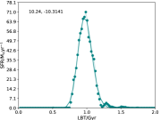
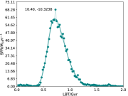
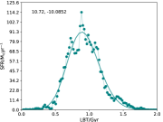
Figure 17: Examples of the star formation histories of $z=3$ massive quiescent galaxies in EAGLE (symbols connected with dotted lines) and the best skewed Gaussian fit (solid line). In each panel we show the $z=3$ stellar mass and “goodness” of fit, as defined in this Appendix. The top three panels show very good fits, while in the middle panel we show galaxies with reasonably good fits, which have small bumps, but which we do not consider as multi-starbursts. The bottom-left panel shows an example of a uni-modal SFHs that is poorly fit by a skewed Gaussian due to the very shark decrease after the peak. We reclassify those as being uni-modal despite the poor goodness of fit. The bottom middle and right panels show galaxies that have a poor fit due to them displaying clear multi-starbursts. The goodness threshold used in EAGLE to separate uni-model vs multiple starbursts is $-9.8$.

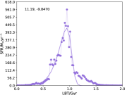
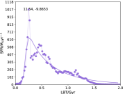
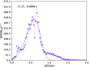
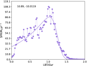
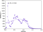
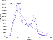
Figure 18: As in Fig. 17 but for Illustris-TNG. The top panel show very good fits, while the middle panels show galaxies with reasonably good fits and small bumps in their SFHs but that we do not consider as being clearly multiple starbursts. The bottom panels show examples of clear multiple starbursts. The goodness threshold used in Illustris-TNG to separate uni-model vs multiple starbursts is $-9.83$.

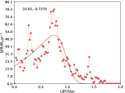
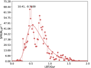
Figure 19: As in Fig. 17 but for Simba. The top panel show very good fits, while the middle panels show galaxies with reasonably good fits and small bumps in their SFHs but that we do not consider as being clear multiple starbursts. The bottom panels show examples of clear multiple starbursts. The goodness threshold used in Simba to separate uni-model vs multiple starbursts is $-9.75$.

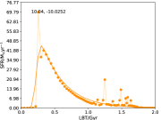
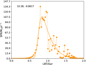
Figure 20: As in Fig. 17 but for Shark. The top $3$ panels show very good fits. The middle left and middle panels show reasonably good fits, with the panel on the left showing a common “saw”-like feature which corresponds to a natural stochasticity in the model. We still classify these as being uni-modal SFHs. The middle-right panel shows an example of a uni-modal SFH that is poorly fit. This happens because the burst is extremely short in duration and is not easily modelled with a skewed Gaussian. We reclassify all of those as being uni-modal despite the goodness of fit being poor. The bottom panels show clear examples of multiple starbursts that were found thanks to the goodness of fit being poor. For Shark, we used a goodness of fit threshold of $-9.7$ to separate SFHs between uni-modal and multi-bursts (a bit lower than the other simulations).

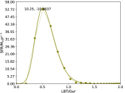
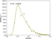
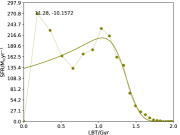
Figure 21: As in Fig. 17 but for GAEA. The top panel show very good fits, while the middle panels show galaxies with reasonably good fits and small bumps in their SFHs but that we do not consider as being clear multiple starbursts. The bottom panels show examples of clear multiple starbursts. The goodness threshold used in GAEA to separate uni-model vs multiple starbursts is $-9.9$ (a bit lower than the other simulations).

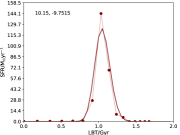
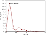
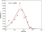
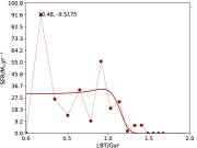
Figure 22: As in Fig. 17 but for Galform. The top panel show very good fits, while the middle panels show galaxies with reasonably good fits and small bumps in their SFHs but that we do not consider as being clear multiple starbursts. The bottom panels show examples of clear multiple starbursts. The goodness threshold used in Galform to separate uni-model vs multiple starbursts is $-9.6$ (a bit higher than the other simulations).

References

- Akins et al. (2022) Akins H. B., Narayanan D., Whitaker K. E., Davé R., Lower S., Bezanson R., Feldmann R., Kriek M., 2022, ApJ, 929, 94
- Alberts et al. (2023) Alberts S., Williams C. C., Helton J. M., Suess K. A., Ji Z., Shivaei I., Lyu J., Rieke G. et al, 2023, arXiv:2312.12207, arXiv:2312.12207
- Anglés-Alcázar et al. (2017) Anglés-Alcázar D., Davé R., Faucher-Giguère C.-A., Özel F., Hopkins P. F., 2017, MNRAS, 464, 2840
- Baugh et al. (2019) Baugh C. M., Gonzalez-Perez V., Lagos C. D. P., Lacey C. G., Helly J. C., Jenkins A., Frenk C. S., Benson A. J. et al, 2019, MNRAS, 483, 4922
- Belli et al. (2019) Belli S., Newman A. B., Ellis R. S., 2019, ApJ, 874, 17
- Benson et al. (2003) Benson A. J., Bower R. G., Frenk C. S., Lacey C. G., Baugh C. M., Cole S., 2003, ApJ, 599, 38
- Bertemes et al. (2024) Bertemes C., Wylezalek D., Rupke D. S. N., Zakamska N. L., Veilleux S., Beckmann B., Vayner A., Sankar S. et al, 2024, arXiv e-prints, arXiv:2404.14475
- Bluck et al. (2020) Bluck A. F. L., Maiolino R., Piotrowska J. M., Trussler J., Ellison S. L., Sánchez S. F., Thorp M. D., Teimoorinia H. et al, 2020, MNRAS, 499, 230
- Bower et al. (2006) Bower R. G., Benson A. J., Malbon R., Helly J. C., Frenk C. S., Baugh C. M., Cole S., Lacey C. G., 2006, MNRAS, 370, 645
- Bower et al. (2017) Bower R. G., Schaye J., Frenk C. S., Theuns T., Schaller M., Crain R. A., McAlpine S., 2017, MNRAS, 465, 32
- Bravo et al. (2022) Bravo M., Robotham A. S. G., Lagos C. d. P., Davies L. J. M., Bellstedt S., Thorne J. E., 2022, MNRAS, 511, 5405
- Bravo et al. (2023) —, 2023, MNRAS, 522, 4481
- Brennan et al. (2018) Brennan R., Choi E., Somerville R. S., Hirschmann M., Naab T., Ostriker J. P., 2018, ApJ, 860, 14
- Bunker et al. (2023) Bunker A. J., Saxena A., Cameron A. J., Willott C. J., Curtis-Lake E., Jakobsen P., Carniani S., Smit R. et al, 2023, A&A, 677, A88
- Carnall et al. (2024) Carnall A. C., Cullen F., McLure R. J., McLeod D. J., Begley R., Donnan C. T., Dunlop J. S., Shapley A. E. et al, 2024, arXiv:2405.02242, arXiv:2405.02242
- Carnall et al. (2023a) Carnall A. C., McLeod D. J., McLure R. J., Dunlop J. S., Begley R., Cullen F., Donnan C. T., Hamadouche M. L. et al, 2023a, MNRAS, 520, 3974
- Carnall et al. (2023b) Carnall A. C., McLure R. J., Dunlop J. S., McLeod D. J., Wild V., Cullen F., Magee D., Begley R. et al, 2023b, Nature, 619, 716
- Carnall et al. (2020) Carnall A. C., Walker S., McLure R. J., Dunlop J. S., McLeod D. J., Cullen F., Wild V., Amorin R. et al, 2020, MNRAS, 496, 695
- Carniani et al. (2024) Carniani S., Hainline K., D’Eugenio F., Eisenstein D. J., Jakobsen P., Witstok J., Johnson B. D., Chevallard J. et al, 2024, arXiv:2405.18485, arXiv:2405.18485
- Castellano et al. (2023) Castellano M., Fontana A., Treu T., Merlin E., Santini P., Bergamini P., Grillo C., Rosati P. et al, 2023, ApJ, 948, L14
- Cattaneo et al. (2008) Cattaneo A., Dekel A., Faber S. M., Guiderdoni B., 2008, MNRAS, 389, 567
- Chabrier (2003) Chabrier G., 2003, PASP, 115, 763
- Clarke et al. (2024) Clarke L., Shapley A. E., Sanders R. L., Topping M. W., Brammer G. B., Bento T., Reddy N. A., Kehoe E., 2024, arXiv e-prints, arXiv:2406.05178
- Correa et al. (2018) Correa C. A., Schaye J., Wyithe J. S. B., Duffy A. R., Theuns T., Crain R. A., Bower R. G., 2018, MNRAS, 473, 538
- Crain et al. (2015) Crain R. A., Schaye J., Bower R. G., Furlong M., Schaller M., Theuns T., Dalla Vecchia C., Frenk C. S. et al, 2015, MNRAS, 450, 1937
- Croton et al. (2006) Croton D. J., Springel V., White S. D. M., De Lucia G., Frenk C. S., Gao L., Jenkins A., Kauffmann G. et al, 2006, MNRAS, 365, 11
- Croton et al. (2016) Croton D. J., Stevens A. R. H., Tonini C., Garel T., Bernyk M., Bibiano A., Hodkinson L., Mutch S. J. et al, 2016, ApJS, 222, 22
- Davé et al. (2019) Davé R., Anglés-Alcázar D., Narayanan D., Li Q., Rafieferantsoa M. H., Appleby S., 2019, MNRAS, 486, 2827
- de Graaff et al. (2024) de Graaff A., Setton D. J., Brammer G., Cutler S., Suess K. A., Labbe I., Leja J., Weibel A. et al, 2024, arXiv e-prints, arXiv:2404.05683
- De Lucia et al. (2011) De Lucia G., Fontanot F., Wilman D., Monaco P., 2011, MNRAS, 414, 1439
- De Lucia et al. (2024) De Lucia G., Fontanot F., Xie L., Hirschmann M., 2024, A&A, 687, A68
- De Lucia et al. (2014) De Lucia G., Tornatore L., Frenk C. S., Helmi A., Navarro J. F., White S. D. M., 2014, MNRAS, 445, 970
- Decarli et al. (2010a) Decarli R., Falomo R., Treves A., Kotilainen J. K., Labita M., Scarpa R., 2010a, MNRAS, 402, 2441
- Decarli et al. (2010b) Decarli R., Falomo R., Treves A., Labita M., Kotilainen J. K., Scarpa R., 2010b, MNRAS, 402, 2453
- Diemer et al. (2017) Diemer B., Sparre M., Abramson L. E., Torrey P., 2017, ApJ, 839, 26
- Driver & Robotham (2010) Driver S. P., Robotham A. S. G., 2010, MNRAS, 407, 2131
- D’Silva et al. (2023a) D’Silva J. C. J., Driver S. P., Lagos C. D. P., Robotham A. S. G., Bellstedt S., Davies L. J. M., Thorne J. E., Bland-Hawthorn J. et al, 2023a, MNRAS
- D’Silva et al. (2023b) —, 2023b, MNRAS, 524, 1448
- D’Silva et al. (2023c) D’Silva J. C. J., Driver S. P., Lagos C. D. P., Robotham A. S. G., Summers J., Windhorst R. A., 2023c, ApJ, 959, L18
- Euclid Collaboration et al. (2024) Euclid Collaboration, Mellier Y., Abdurro’uf, Acevedo Barroso J. A., Achúcarro A., Adamek J., Adam R., Addison G. E. et al, 2024, arXiv e-prints, arXiv:2405.13491
- Fontanot et al. (2020) Fontanot F., De Lucia G., Hirschmann M., Xie L., Monaco P., Menci N., Fiore F., Feruglio C. et al, 2020, MNRAS, 496, 3943
- Franx et al. (2008) Franx M., van Dokkum P. G., Förster Schreiber N. M., Wuyts S., Labbé I., Toft S., 2008, ApJ, 688, 770
- Furtak et al. (2024) Furtak L. J., Labbé I., Zitrin A., Greene J. E., Dayal P., Chemerynska I., Kokorev V., Miller T. B. et al, 2024, Nature, 628, 57
- Girelli et al. (2019) Girelli G., Bolzonella M., Cimatti A., 2019, A&A, 632, A80
- Glazebrook et al. (2024) Glazebrook K., Nanayakkara T., Schreiber C., Lagos C., Kawinwanichakij L., Jacobs C., Chittenden H., Brammer G. et al, 2024, Nature, 628, 277
- Glazebrook et al. (2017) Glazebrook K., Schreiber C., Labbé I., Nanayakkara T., Kacprzak G. G., Oesch P. A., Papovich C., Spitler L. R. et al, 2017, Nature, 544, 71
- Golubchik et al. (2024) Golubchik M., Steinhardt C. L., Zitrin A., Meena A. K., Furtak L. J., Chelouche D., Kaspi S., 2024, arXiv:2408.00073, arXiv:2408.00073
- Gould et al. (2023) Gould K. M. L., Brammer G., Valentino F., Whitaker K. E., Weaver J. R., Lagos C. d. P., Rizzo F., Franco M. et al, 2023, AJ, 165, 248
- Hartley et al. (2023) Hartley A. I., Nelson E. J., Suess K. A., Garcia A. M., Park M., Hernquist L., Bezanson R., Nevin R. et al, 2023, MNRAS, 522, 3138
- Henriques et al. (2015) Henriques B. M. B., White S. D. M., Thomas P. A., Angulo R., Guo Q., Lemson G., Springel V., Overzier R., 2015, MNRAS, 451, 2663
- Hirschmann et al. (2016) Hirschmann M., De Lucia G., Fontanot F., 2016, MNRAS, 461, 1760
- Hopkins (2015) Hopkins P. F., 2015, MNRAS, 450, 53
- Hopkins (2017) —, 2017, arXiv e-prints, arXiv:1712.01294
- Ishibashi & Fabian (2015) Ishibashi W., Fabian A. C., 2015, MNRAS, 451, 93
- Jiang et al. (2014) Jiang L., Helly J. C., Cole S., Frenk C. S., 2014, MNRAS, 440, 2115
- Kennicutt (1983) Kennicutt Jr. R. C., 1983, ApJ, 272, 54
- Kimmig et al. (2023) Kimmig L. C., Remus R.-S., Seidel B., Valenzuela L. M., Dolag K., Burkert A., 2023, arXiv e-prints, arXiv:2310.16085
- Komatsu et al. (2011) Komatsu E., Smith K. M., Dunkley J., Bennett C. L., Gold B., Hinshaw G., Jarosik N., Larson D. et al, 2011, ApJS, 192, 18
- Kugel et al. (2023) Kugel R., Schaye J., Schaller M., Helly J. C., Braspenning J., Elbers W., Frenk C. S., McCarthy I. G. et al, 2023, MNRAS, 526, 6103
- Kurinchi-Vendhan et al. (2023) Kurinchi-Vendhan S., Farcy M., Hirschmann M., Valentino F., 2023, arXiv e-prints, arXiv:2310.03083
- Lacey et al. (2016) Lacey C. G., Baugh C. M., Frenk C. S., Benson A. J., Bower R. G., Cole S., Gonzalez-Perez V., Helly J. C. et al, 2016, MNRAS, 462, 3854
- Lagos et al. (2024) Lagos C. d. P., Bravo M., Tobar R., Obreschkow D., Power C., Robotham A. S. G., Proctor K. L., Hansen S. et al, 2024, MNRAS, 531, 3551
- Lagos et al. (2008) Lagos C. D. P., Cora S. A., Padilla N. D., 2008, MNRAS, 388, 587
- Lagos et al. (2018) Lagos C. d. P., Tobar R. J., Robotham A. S. G., Obreschkow D., Mitchell P. D., Power C., Elahi P. J., 2018, ArXiv:1807.11180
- Long et al. (2023) Long A. S., Antwi-Danso J., Lambrides E. L., Lovell C. C., de la Vega A., Valentino F., Zavala J. A., Casey C. M. et al, 2023, arXiv e-prints, arXiv:2305.04662
- Looser et al. (2023) Looser T. J., D’Eugenio F., Maiolino R., Tacchella S., Curti M., Arribas S., Baker W. M., Baum S. et al, 2023, arXiv e-prints, arXiv:2306.02470
- Lustig et al. (2023) Lustig P., Strazzullo V., Remus R.-S., D’Eugenio C., Daddi E., Burkert A., De Lucia G., Delvecchio I. et al, 2023, MNRAS, 518, 5953
- Manning et al. (2022) Manning S. M., Casey C. M., Zavala J. A., Magdis G. E., Drew P. M., Champagne J. B., Aravena M., Béthermin M. et al, 2022, ApJ, 925, 23
- McAlpine et al. (2015) McAlpine S., Helly J. C., Schaller M., Trayford J. W., Qu Y., Furlong M., Bower R. G., Crain R. A. et al, 2015, ArXiv:1510.01320
- Merlin et al. (2019) Merlin E., Fortuni F., Torelli M., Santini P., Castellano M., Fontana A., Grazian A., Pentericci L. et al, 2019, MNRAS, 490, 3309
- Mun et al. (2024) Mun M., Wisnioski E., Battisti A. J., Mendel J. T., Ellison S. L., Taylor E. N., Lagos C. D. P., Harborne K. E. et al, 2024, MNRAS, 530, 5072
- Nanayakkara et al. (2024) Nanayakkara T., Glazebrook K., Jacobs C., Kawinwanichakij L., Schreiber C., Brammer G., Esdaile J., Kacprzak G. G. et al, 2024, Scientific Reports, 14, 3724
- Nelson et al. (2019) Nelson D., Springel V., Pillepich A., Rodriguez-Gomez V., Torrey P., Genel S., Vogelsberger M., Pakmor R. et al, 2019, Computational Astrophysics and Cosmology, 6, 2
- Pacifici et al. (2023) Pacifici C., Iyer K. G., Mobasher B., da Cunha E., Acquaviva V., Burgarella D., Calistro Rivera G., Carnall A. C. et al, 2023, ApJ, 944, 141
- Pakmor et al. (2011) Pakmor R., Bauer A., Springel V., 2011, MNRAS, 418, 1392
- Pillepich et al. (2018) Pillepich A., Springel V., Nelson D., Genel S., Naiman J., Pakmor R., Hernquist L., Torrey P. et al, 2018, MNRAS, 473, 4077
- Planck Collaboration (2014) Planck Collaboration, 2014, A&A, 571, A16
- Planck Collaboration et al. (2016) Planck Collaboration, Ade P. A. R., Aghanim N., Arnaud M., Ashdown M., Aumont J., Baccigalupi C., Banday A. J. et al, 2016, A&A, 594, A13
- Poitevineau et al. (2023) Poitevineau R., Castignani G., Combes F., 2023, A&A, 672, A164
- Poulton et al. (2021) Poulton R. J. J., Power C., Robotham A. S. G., Elahi P. J., Lagos C. D. P., 2021, MNRAS, 501, 2810
- Remus & Kimmig (2023) Remus R.-S., Kimmig L. C., 2023, arXiv e-prints, arXiv:2310.16089
- Robotham et al. (2020) Robotham A. S. G., Bellstedt S., Lagos C. d. P., Thorne J. E., Davies L. J., Driver S. P., Bravo M., 2020, MNRAS, 495, 905
- Schaller et al. (2015) Schaller M., Frenk C. S., Bower R. G., Theuns T., Jenkins A., Schaye J., Crain R. A., Furlong M. et al, 2015, MNRAS, 451, 1247
- Schaye et al. (2015) Schaye J., Crain R. A., Bower R. G., Furlong M., Schaller M., Theuns T., Dalla Vecchia C., Frenk C. S. et al, 2015, MNRAS, 446, 521
- Schreiber et al. (2018) Schreiber C., Glazebrook K., Nanayakkara T., Kacprzak G. G., Labbé I., Oesch P., Yuan T., Tran K. V. et al, 2018, A&A, 618, A85
- Schreiber et al. (2015) Schreiber C., Pannella M., Elbaz D., Béthermin M., Inami H., Dickinson M., Magnelli B., Wang T. et al, 2015, A&A, 575, A74
- Shahidi et al. (2020) Shahidi A., Mobasher B., Nayyeri H., Hemmati S., Wiklind T., Chartab N., Dickinson M., Finkelstein S. L. et al, 2020, ApJ, 897, 44
- Sijacki et al. (2007) Sijacki D., Springel V., Di Matteo T., Hernquist L., 2007, MNRAS, 380, 877
- Somerville et al. (2008) Somerville R. S., Hopkins P. F., Cox T. J., Robertson B. E., Hernquist L., 2008, MNRAS, 391, 481
- Somerville et al. (2015) Somerville R. S., Popping G., Trager S. C., 2015, MNRAS, 453, 4337
- Springel (2005) Springel V., 2005, MNRAS, 364, 1105
- Springel (2010) Springel V., 2010, MNRAS, 401, 791
- Springel et al. (2018) Springel V., Pakmor R., Pillepich A., Weinberger R., Nelson D., Hernquist L., Vogelsberger M., Genel S. et al, 2018, MNRAS, 475, 676
- Springel et al. (2008) Springel V., Wang J., Vogelsberger M., Ludlow A., Jenkins A., Helmi A., Navarro J. F., Frenk C. S. et al, 2008, MNRAS, 391, 1685
- Springel et al. (2005) Springel V., White S. D. M., Jenkins A., Frenk C. S., Yoshida N., Gao L., Navarro J., Thacker R. et al, 2005, Nature, 435, 629
- Springel et al. (2001) Springel V., White S. D. M., Tormen G., Kauffmann G., 2001, MNRAS, 328, 726
- Straatman et al. (2014) Straatman C. M. S., Labbé I., Spitler L. R., Allen R., Altieri B., Brammer G. B., Dickinson M., van Dokkum P. et al, 2014, ApJ, 783, L14
- Suh et al. (2020) Suh H., Civano F., Trakhtenbrot B., Shankar F., Hasinger G., Sanders D. B., Allevato V., 2020, ApJ, 889, 32
- Szpila et al. (2024) Szpila J., Davé R., Rennehan D., Cui W., Hough R., 2024, arXiv e-prints, arXiv:2402.08729
- Terrazas et al. (2020) Terrazas B. A., Bell E. F., Pillepich A., Nelson D., Somerville R. S., Genel S., Weinberger R., Habouzit M. et al, 2020, MNRAS, 493, 1888
- Terrazas et al. (2017) Terrazas B. A., Bell E. F., Woo J., Henriques B. M. B., 2017, ApJ, 844, 170
- The EAGLE team (2017) The EAGLE team, 2017, arXiv e-prints, arXiv:1706.09899
- Thomas et al. (2021) Thomas N., Davé R., Jarvis M. J., Anglés-Alcázar D., 2021, MNRAS, 503, 3492
- Thorne et al. (2021) Thorne J. E., Robotham A. S. G., Davies L. J. M., Bellstedt S., Driver S. P., Bravo M., Bremer M. N., Holwerda B. W. et al, 2021, MNRAS, 505, 540
- Trayford et al. (2016) Trayford J. W., Theuns T., Bower R. G., Crain R. A., Lagos C. d. P., Schaller M., Schaye J., 2016, MNRAS, 460, 3925
- Valentino et al. (2023) Valentino F., Brammer G., Gould K. M. L., Kokorev V., Fujimoto S., Jespersen C. K., Vijayan A. P., Weaver J. R. et al, 2023, ApJ, 947, 20
- Valentino et al. (2020) Valentino F., Tanaka M., Davidzon I., Toft S., Gómez-Guijarro C., Stockmann M., Onodera M., Brammer G. et al, 2020, ApJ, 889, 93
- Vani et al. (2024) Vani A., Ayromlou M., Kauffmann G., Springel V., 2024, arXiv e-prints, arXiv:2408.00824
- Wang et al. (2024) Wang T., Sun H., Zhou L., Xu K., Cheng C., Li Z., Chen Y., Mo H. J. et al, 2024, arXiv e-prints, arXiv:2403.02399
- Weaver et al. (2023) Weaver J. R., Davidzon I., Toft S., Ilbert O., McCracken H. J., Gould K. M. L., Jespersen C. K., Steinhardt C. et al, 2023, A&A, 677, A184
- Weibel et al. (2024) Weibel A., de Graaff A., Setton D. J., Miller T. B., Oesch P. A., Brammer G., Lagos C. D. P., Whitaker K. E. et al, 2024, arXiv:2409.03829, arXiv:2409.03829
- Weinberger et al. (2017) Weinberger R., Springel V., Hernquist L., Pillepich A., Marinacci F., Pakmor R., Nelson D., Genel S. et al, 2017, MNRAS, 465, 3291
- Weinberger et al. (2020) Weinberger R., Springel V., Pakmor R., 2020, ApJS, 248, 32
- Weinberger et al. (2018) Weinberger R., Springel V., Pakmor R., Nelson D., Genel S., Pillepich A., Vogelsberger M., Marinacci F. et al, 2018, MNRAS, 479, 4056
- Weller et al. (2024) Weller E. J., Pacucci F., Ni Y., Hernquist L., Park M., 2024, arXiv:2406.02664, arXiv:2406.02664
- Wright et al. (2019) Wright R. J., Lagos C. d. P., Davies L. J. M., Power C., Trayford J. W., Wong O. I., 2019, MNRAS, 487, 3740
- Wright et al. (2024) Wright R. J., Somerville R. S., Lagos C. d. P., Schaller M., Davé R., Anglés-Alcázar D., Genel S., 2024, arXiv e-prints, arXiv:2402.08408