Importance Sampling for the Extremal Eigenvalue of β𝛽\beta-Jacobi ensemble

Yutao Ma Yutao MA
School of Mathematical Sciences &\& Laboratory of Mathematics and Complex Systems of Ministry of Education, Beijing Normal University, 100875 Beijing, China.
mayt@bnu.edu.cn
Β andΒ  Siyu Wang Siyu Wang
School of Mathematical Sciences &\& Laboratory of Mathematics and Complex Systems of Ministry of Education, Beijing Normal University, 100875 Beijing, China.
wang_siyu@mail.bnu.edu.cn
Abstract.

This paper focuses on rare events associated with the tail probabilities of the extremal eigenvalues in the β𝛽\beta-Jacobi ensemble, which plays a critical role in both multivariate statistical analysis and statistical physics. Under the ultra-high dimensional setting, we give an exact approximation for the tail probabilities and construct an efficient estimator for the tail probabilities. Additionally, we conduct a numerical study to evaluate the practical performance of our algorithms. The simulation results demonstrate that our method offers an efficient and accurate approach for evaluating tail probabilities in practice.

The research of Yutao Ma was supported in part by NSFC 12171038, 11871008 and 985 Projects.

Keywords: importance sampling; extremal eigenvalue; β𝛽\beta-Jacobi ensemble.

AMS Classification Subjects 2020: 60F10, 60B20

1. Introduction

In classical multivariate analysis, the tail probabilities of the largest eigenvalues play a crucial role and are widely applied to various statistical problems, such as linear regression, MANOVA (Multivariate Analysis of Variance), canonical correlation analysis, and the equality of covariance matrices. This paper focuses on the tail probabilities of the largest eigenvalues of the β𝛽\beta-Jacobi ensemble, whose density function is given in equation (1.1).

Specifically, when Ξ²=1𝛽1\beta=1, the β𝛽\beta-Jacobi ensemble corresponds to the eigenvalue distribution of real MANOVA matrices ([19]). Consider an nΓ—p1𝑛subscript𝑝1n\times p_{1} normal data matrix X,𝑋X, where each row is an independent observation from 𝒩​(0,Ξ£).𝒩0Ξ£\mathcal{N}(0,\Sigma). The matrix A=X′​X𝐴superscript𝑋′𝑋A=X^{\prime}X follows a Wishart distribution, A∼Wn​(Ξ£,p1),similar-to𝐴subscriptπ‘Šπ‘›Ξ£subscript𝑝1A\sim W_{n}(\Sigma,p_{1}), and let B∼Wn​(Ξ£,p2),similar-to𝐡subscriptπ‘Šπ‘›Ξ£subscript𝑝2B\sim W_{n}(\Sigma,p_{2}), independent of A.𝐴A. Then, the distribution of MANOVA matrix (A+B)βˆ’1​Bsuperscript𝐴𝐡1𝐡(A+B)^{-1}B follows equation (1.1)(with Ξ²=1𝛽1\beta=1). When the elements of X𝑋X are complex or quaternion, the cases Ξ²=2𝛽2\beta=2 and Ξ²=4𝛽4\beta=4 correspond to the eigenvalue distributions of complex and quaternion MANOVA matrices, respectively. The distribution of the largest eigenvalue of the MANOVA matrix has broad applications in multivariate statistical analysis. For instance, Johnstone’s work ([13]) on the convergence of the largest eigenvalue has been used to address several classic problems in multivariate statistics. In canonical correlation analysis, the largest eigenvalue quantifies the linear relationship between two sets of variables; in the analysis of angles and distances between subspaces, it assesses the similarity between high-dimensional datasets; in multivariate linear models, it tests the significance of linear hypotheses; in testing the equality of covariance matrices, the largest eigenvalue is used to compare the covariance structures across different groups; and in multiple discriminant analysis, it measures the separability between categories, thereby improving the accuracy of group classification.

For general Ξ²>0,𝛽0\beta>0, the β𝛽\beta-Jacobi ensemble can be viewed as a non-equilibrium system in statistical physics, where β𝛽\beta serves as the inverse temperature, controlling the interaction strength between eigenvalues. In the study of energy spectrum distributions and phase transition behavior, the largest eigenvalue of the β𝛽\beta-Jacobi ensemble plays a crucial role in describing the system’s extreme behavior in different energy states, while also revealing the characteristics of critical points during phase transitions.

In the study of the aforementioned multivariate statistical analyses and statistical physics models, sampling from the event {Ξ»max>x}subscriptπœ†maxπ‘₯\{\lambda_{\text{max}}>x\} is often required. For general Ξ²>0,𝛽0\beta>0, Killip and Nenciu ([15]) constructed a tridiagonal random matrix model for the β𝛽\beta-Jacobi ensemble. Using this model, the eigenvalues of the tridiagonal matrix can be computed via Monte Carlo methods to simulate the behavior of Ξ»max.subscriptπœ†max\lambda_{\text{max}}. However, when the probability of the event {Ξ»max>x}subscriptπœ†maxπ‘₯\{\lambda_{\text{max}}>x\} is extremely small or the data dimension is very large, direct Monte Carlo simulations become highly inefficient. These simulations require substantially larger sample sizes, resulting in a significant increase in computational cost.

Large deviation theory provides a valuable tool for quantifying the probabilities of rare events ([22]). However, practical applications face challenges, as approximations based on large deviation results may lack direct applicability, leading to insufficient accuracy in estimating the probabilities of rare events. In this context, importance sampling emerges as the preferred approach. Unlike classical Monte Carlo methods, importance sampling significantly reduces simulation time and improves efficiency. Essentially, importance sampling is a modified Monte Carlo technique that produces estimates with a smaller coefficient of variation–a natural performance metric for rare event estimation.

The focus of this paper is to construct an effective estimator for the tail probabilities of the β𝛽\beta-Jacobi ensemble using importance sampling. Asmussen and Kroese ([1]) addressed the problem of tail probability estimation for independent and identically distributed heavy-tailed random variables, developing importance sampling estimators through a two-step construction. Building on a similar structural approach, Jiang et al. ([11]) delved into the asymptotical behavior of top eigenvalues for the β𝛽\beta-Laguerre ensemble, using the tridiagonal random matrix characterization of the β𝛽\beta-Laguerre ensemble and the β€œthree-step peeling” technique to precisely estimate the tail probability. Inspired by Jiang et al. ([11]), we previously constructed an asymptotically effective estimator for the tail probabilities of the β𝛽\beta-Jacobi ensemble in [18]. In this paper, we take this further by constructing a strongly efficient estimator for the tail probabilities.

A β𝛽\beta-Jacobi ensemble π’₯n​(p1,p2)subscriptπ’₯𝑛subscript𝑝1subscript𝑝2\mathcal{J}_{n}(p_{1},p_{2}) is a set of random variables Ξ»:=(Ξ»1,Ξ»2,β‹―,Ξ»n)∈[0,1]nassignπœ†subscriptπœ†1subscriptπœ†2β‹―subscriptπœ†π‘›superscript01𝑛\lambda:=\left(\lambda_{1},\lambda_{2},\cdots,\lambda_{n}\right)\in[0,1]^{n} with joint probability density function

(1.1) fnp1,p2​(x1,β‹―,xn)=Cnp1,p2β€‹βˆ1≀i<j≀n|xiβˆ’xj|Ξ²β€‹βˆi=1nxir1,nβˆ’1​(1βˆ’xi)r2,nβˆ’1,superscriptsubscript𝑓𝑛subscript𝑝1subscript𝑝2subscriptπ‘₯1β‹―subscriptπ‘₯𝑛superscriptsubscript𝐢𝑛subscript𝑝1subscript𝑝2subscriptproduct1𝑖𝑗𝑛superscriptsubscriptπ‘₯𝑖subscriptπ‘₯𝑗𝛽superscriptsubscriptproduct𝑖1𝑛superscriptsubscriptπ‘₯𝑖subscriptπ‘Ÿ1𝑛1superscript1subscriptπ‘₯𝑖subscriptπ‘Ÿ2𝑛1\displaystyle f_{n}^{p_{1},p_{2}}\left(x_{1},\cdots,x_{n}\right)=C_{n}^{p_{1},p_{2}}\prod_{1\leq i<j\leq n}\left|x_{i}-x_{j}\right|^{\beta}\prod_{i=1}^{n}x_{i}^{r_{1,n}-1}\left(1-x_{i}\right)^{r_{2,n}-1},

where p1,p2β‰₯n,ri,n:=β​(piβˆ’n+1)2formulae-sequencesubscript𝑝1subscript𝑝2𝑛assignsubscriptπ‘Ÿπ‘–π‘›π›½subscript𝑝𝑖𝑛12p_{1},p_{2}\geq n,r_{i,n}:=\frac{\beta\left(p_{i}-n+1\right)}{2} for i=1,2𝑖12i=1,2 and Ξ²>0𝛽0\beta>0, and the normalizing constant Cnp1,p2superscriptsubscript𝐢𝑛subscript𝑝1subscript𝑝2C_{n}^{p_{1},p_{2}} is given by

Cnp1,p2=∏j=1nΓ​(1+Ξ²2)​Γ​(Ξ²(pβˆ’n+j2)Γ​(1+β​j2)​Γ​(β​(p1βˆ’n+j)2)​Γ​(β​(p2βˆ’n+j)2)C_{n}^{p_{1},p_{2}}=\prod_{j=1}^{n}\frac{\Gamma\left(1+\frac{\beta}{2}\right)\Gamma\left(\frac{\beta(p-n+j}{2}\right)}{\Gamma\left(1+\frac{\beta j}{2}\right)\Gamma\left(\frac{\beta\left(p_{1}-n+j\right)}{2}\right)\Gamma\left(\frac{\beta\left(p_{2}-n+j\right)}{2}\right)}

with p=p1+p2𝑝subscript𝑝1subscript𝑝2p=p_{1}+p_{2} and Γ​(a)=∫0∞xaβˆ’1​eβˆ’x​𝑑xΞ“π‘Žsuperscriptsubscript0superscriptπ‘₯π‘Ž1superscript𝑒π‘₯differential-dπ‘₯\Gamma(a)=\int_{0}^{\infty}x^{a-1}e^{-x}dx with a>0.π‘Ž0a>0. Let Ξ»(1)<Ξ»(2)<β‹―<Ξ»(n)subscriptπœ†1subscriptπœ†2β‹―subscriptπœ†π‘›\lambda_{(1)}<\lambda_{(2)}<\cdots<\lambda_{(n)} be the order statistics of the β𝛽\beta-Jacobi ensemble π’₯n​(p1,p2)subscriptπ’₯𝑛subscript𝑝1subscript𝑝2\mathcal{J}_{n}(p_{1},p_{2}), with joint distribution Gnp1,p2superscriptsubscript𝐺𝑛subscript𝑝1subscript𝑝2G_{n}^{p_{1},p_{2}} and joint density function

(1.2) n!​fnp1,p2​(x1,β‹―,xn)β€‹πŸ(x1<β‹―<xn).𝑛superscriptsubscript𝑓𝑛subscript𝑝1subscript𝑝2subscriptπ‘₯1β‹―subscriptπ‘₯𝑛subscript1subscriptπ‘₯1β‹―subscriptπ‘₯𝑛\displaystyle n!f_{n}^{p_{1},p_{2}}\left(x_{1},\cdots,x_{n}\right)\mathbf{1}_{\left(x_{1}<\cdots<x_{n}\right)}.

In this paper, we provide asymptotic approximations for the tail probabilities ℙ​(Ξ»(n)>p1p​x)β„™subscriptπœ†π‘›subscript𝑝1𝑝π‘₯\mathbb{P}\left(\lambda_{(n)}>\frac{p_{1}}{p}x\right) of the extremal eigenvalues under certain conditions on β𝛽\beta, n𝑛n, p1subscript𝑝1p_{1}, and p2subscript𝑝2p_{2}. Moreover, we construct efficient Monte Carlo simulation algorithms to compute the tail probabilities. In the following sections, we introduce the fundamental setup for importance sampling and present the main results of our paper.

2. Tail Probability Estimation

2.1. Basic importance sampling

Consider a random variable Yπ‘ŒY with probability distribution Q𝑄Q taking values on spaces ΩΩ\Omega, and a real-valued function Ο‰πœ”\omega on ΩΩ\Omega. Importance sampling is based on the basic identity, for fixed Bβˆˆβ„¬,𝐡ℬB\in\mathcal{B},

𝔼​[𝟏{ω​(Y)∈B}]=𝔼R​[𝟏{ω​(Y)∈B}​d​Qd​R],𝔼delimited-[]subscript1πœ”π‘Œπ΅superscript𝔼𝑅delimited-[]subscript1πœ”π‘Œπ΅d𝑄d𝑅\mathbb{E}\left[\mathbf{1}_{\left\{\omega\left(Y\right)\in B\right\}}\right]=\mathbb{E}^{R}\left[\mathbf{1}_{\left\{\omega\left(Y\right)\in B\right\}}\frac{\mathrm{d}Q}{\mathrm{d}R}\right],

where R𝑅R is a probability measure such that the Radon-Nikodym derivative d​Q/d​Rd𝑄d𝑅\mathrm{d}Q/\mathrm{d}R is well defined on the set {ω​(Y)∈B}πœ”π‘Œπ΅\left\{\omega\left(Y\right)\in B\right\}. Here, ℬℬ\mathcal{B} denotes the Borel ΟƒπœŽ\sigma-algebra on ℝℝ\mathbb{R}, and 𝔼𝔼\mathbb{E} or 𝔼Rsuperscript𝔼𝑅\mathbb{E}^{R} denotes the expectations under the measures Q𝑄Q or R𝑅R, respectively. Then, the random variable F𝐹F is given by

(2.1) F=d​Qd​Rβ€‹πŸ{ω​(Y)∈B}𝐹d𝑄d𝑅subscript1πœ”π‘Œπ΅\displaystyle F=\frac{\mathrm{d}Q}{\mathrm{d}R}\mathbf{1}_{\left\{\omega\left(Y\right)\in B\right\}}

is an unbiased estimator of ℙ​(ω​(Y)∈B)β„™πœ”π‘Œπ΅\mathbb{P}\left(\omega\left(Y\right)\in B\right) under the measure R𝑅R. An averaged importance sampling estimator based on the measure Q𝑄Q is obtained by simulating N𝑁N i.i.d. copies F(1),…,F(N)superscript𝐹1…superscript𝐹𝑁F^{(1)},\ldots,F^{(N)} of F𝐹F under R𝑅R and computing the empirical average F^N=(F(1)+β‹―+F(N))/Nsubscript^𝐹𝑁superscript𝐹1β‹―superscript𝐹𝑁𝑁\widehat{F}_{N}=\left(F^{(1)}+\cdots+F^{(N)}\right)/N. Moreover, its variance is

VarR​(F^N)=𝔼R​[F2]βˆ’β„™β€‹(ω​(Y)∈B)2N,superscriptVar𝑅subscript^𝐹𝑁superscript𝔼𝑅delimited-[]superscript𝐹2β„™superscriptπœ”π‘Œπ΅2𝑁\mathrm{Var}^{R}\left(\widehat{F}_{N}\right)=\frac{\mathbb{E}^{R}\left[F^{2}\right]-\mathbb{P}\left(\omega\left(Y\right)\in B\right)^{2}}{N},

which decreases as N𝑁N increases. The coefficient of variation is given by

(2.2) C.O.V.(F^N):=VarR​(F^N)𝔼R​(F^N)=1N​(𝔼R​[F2]ℙ​(ω​(Y)∈B)2βˆ’1)1/2.formulae-sequenceCOVassignsubscript^𝐹𝑁superscriptVar𝑅subscript^𝐹𝑁superscript𝔼𝑅subscript^𝐹𝑁1𝑁superscriptsuperscript𝔼𝑅delimited-[]superscript𝐹2β„™superscriptπœ”π‘Œπ΅2112\displaystyle\mathrm{C.O.V.}\left(\widehat{F}_{N}\right):=\frac{\sqrt{\mathrm{Var}^{R}\left(\widehat{F}_{N}\right)}}{\mathbb{E}^{R}\left(\widehat{F}_{N}\right)}=\frac{1}{\sqrt{N}}\left(\frac{\mathbb{E}^{R}\left[F^{2}\right]}{\mathbb{P}\left(\omega\left(Y\right)\in B\right)^{2}}-1\right)^{1/2}.

A central issue is to optimize the left-hand side of (2.2) via selecting R.𝑅R. In the case that R𝑅R is taken as

Rβˆ—(β‹…):=β„™(β‹…βˆ£Ο‰(Y)∈B),R^{*}(\cdot):=\mathbb{P}\left(\cdot\mid\omega\left(Y\right)\in B\right),

it turns out that

VarR​(F^N)=0.superscriptVar𝑅subscript^𝐹𝑁0{\rm Var}^{R}(\widehat{F}_{N})=0.

Unfortunately, the optimal IS density Rβˆ—superscript𝑅R^{*} is computationally unavailable since we do not know the value of ℙ​(ω​(Y)∈B).β„™πœ”π‘Œπ΅\mathbb{P}\left(\omega\left(Y\right)\in B\right).

Given a family of Borel sets (Bn;nβ‰₯1)subscript𝐡𝑛𝑛1(B_{n};n\geq 1) such that

0<ℙ​(ω​(Y)∈Bn)​ and ​limnβ†’βˆžβ„™β€‹(ω​(Y)∈Bn)=0,0β„™πœ”π‘Œsubscript𝐡𝑛 andΒ subscriptβ†’π‘›β„™πœ”π‘Œsubscript𝐡𝑛00<\mathbb{P}\left(\omega\left(Y\right)\in B_{n}\right)\text{ and }\lim_{n\to\infty}\mathbb{P}\left(\omega\left(Y\right)\in B_{n}\right)=0,

it is necessary to consider the quotient

𝔼R​[Fn2]ℙ​(ω​(Y)∈B)2superscript𝔼𝑅delimited-[]superscriptsubscript𝐹𝑛2β„™superscriptπœ”π‘Œπ΅2\frac{\mathbb{E}^{R}\left[F_{n}^{2}\right]}{\mathbb{P}\left(\omega\left(Y\right)\in B\right)^{2}}

when constructing a sequence of estimators (Fn;nβ‰₯1)subscript𝐹𝑛𝑛1(F_{n};n\geq 1) for ℙ​(ω​(Y)∈Bn)β„™πœ”π‘Œsubscript𝐡𝑛\mathbb{P}\left(\omega\left(Y\right)\in B_{n}\right). In the context of rare-event simulations (e.g., Asmussen and Glynn, [2]), they say that Fnsubscript𝐹𝑛F_{n} is strongly efficient if

(2.3) limΒ―nβ†’βˆžβ‘π”ΌR​[Fn2]ℙ​(ω​(Y)∈Bn)2<∞.subscriptlimit-supremum→𝑛superscript𝔼𝑅delimited-[]superscriptsubscript𝐹𝑛2β„™superscriptπœ”π‘Œsubscript𝐡𝑛2\displaystyle\varlimsup_{n\rightarrow\infty}\frac{\mathbb{E}^{R}\left[F_{n}^{2}\right]}{\mathbb{P}\left(\omega\left(Y\right)\in B_{n}\right)^{2}}<\infty.

Another efficiency concept slightly weaker than strongly efficient is asymptotically (or logarithmically) efficient: 𝔼R​[Fn2]superscript𝔼𝑅delimited-[]superscriptsubscript𝐹𝑛2\mathbb{E}^{R}\left[F_{n}^{2}\right] tends to 00 so fast that

limnβ†’βˆž|log⁑𝔼R​[Fn2]|2​|log⁑ℙ​(ω​(Y)∈Bn)|=1.subscript→𝑛superscript𝔼𝑅delimited-[]superscriptsubscript𝐹𝑛22β„™πœ”π‘Œsubscript𝐡𝑛1\lim_{n\rightarrow\infty}\frac{\left|\log\mathbb{E}^{R}\left[F_{n}^{2}\right]\right|}{2\left|\log\mathbb{P}\left(\omega\left(Y\right)\in B_{n}\right)\right|}=1.

For a detailed discussion on efficiency in rare-event simulations, see Asmussen and Glynn [2], Bucklew [3], or Juneja and Shahabuddin [14].

Constructing efficient estimators for the tail probabilities of the β𝛽\beta-Jacobi ensemble simplifies the computation of extreme value probabilities in applications across multivariate statistical analysis and statistical physics. Strongly efficient estimators offer greater stability, consistency, and accuracy, though they often require more stringent parameter conditions. In contrast, asymptotically efficient estimators typically have lower computational costs, especially in large sample scenarios, making them a more practical choice when computational resources are limited.

2.2. Importance sampling estimator for p​λ(n)/p1𝑝subscriptπœ†π‘›subscript𝑝1p\lambda_{(n)}/p_{1}

Next, we construct the IS estimator Fnsubscript𝐹𝑛F_{n} for ℙ​(Ξ»(n)>p1p​x)β„™subscriptπœ†π‘›subscript𝑝1𝑝π‘₯\mathbb{P}\left(\lambda_{(n)}>\frac{p_{1}}{p}x\right) when x>1π‘₯1x>1. Consider the order statistics (Ξ»~(1),β‹―,Ξ»~(nβˆ’1))subscript~πœ†1β‹―subscript~πœ†π‘›1\left(\widetilde{\lambda}_{(1)},\cdots,\widetilde{\lambda}_{(n-1)}\right) of the β𝛽\beta-Jacobi ensemble π’₯nβˆ’1​(p1βˆ’1,p2βˆ’1)subscriptπ’₯𝑛1subscript𝑝11subscript𝑝21\mathcal{J}_{n-1}(p_{1}-1,p_{2}-1). Let Ξ»~nsubscript~πœ†π‘›\widetilde{\lambda}_{n} be a random variable with conditional density function

(2.4) h​(y):=r1βˆ’eβˆ’r​(1βˆ’p1​x/p∨λ~(nβˆ’1))​eβˆ’r​(yβˆ’(p1​x/p)∨λ~(nβˆ’1))β€‹πŸ{(p1​x/p)∨λ~(nβˆ’1)<y<1},assignβ„Žπ‘¦π‘Ÿ1superscriptπ‘’π‘Ÿ1subscript𝑝1π‘₯𝑝subscript~πœ†π‘›1superscriptπ‘’π‘Ÿπ‘¦subscript𝑝1π‘₯𝑝subscript~πœ†π‘›1subscript1subscript𝑝1π‘₯𝑝subscript~πœ†π‘›1𝑦1h\left(y\right):=\frac{r}{1-e^{-r(1-p_{1}x/p\vee\widetilde{\lambda}_{(n-1)})}}e^{-r\left(y-\left(p_{1}x/p\right)\vee\widetilde{\lambda}_{(n-1)}\right)}\mathbf{1}_{\{\left(p_{1}x/p\right)\vee\widetilde{\lambda}_{(n-1)}<y<1\}},

given (Ξ»~(1),β‹―,Ξ»~(nβˆ’1)),subscript~πœ†1β‹―subscript~πœ†π‘›1\left(\widetilde{\lambda}_{(1)},\cdots,\widetilde{\lambda}_{(n-1)}\right), where the rate r=β​p​(xβˆ’1)2​x.π‘Ÿπ›½π‘π‘₯12π‘₯r=\frac{\beta p(x-1)}{2x}. Let Lnp1,p2superscriptsubscript𝐿𝑛subscript𝑝1subscript𝑝2L_{n}^{p_{1},p_{2}} be the joint distribution of (Ξ»~(1),β‹―,Ξ»~(nβˆ’1),Ξ»~n).subscript~πœ†1β‹―subscript~πœ†π‘›1subscript~πœ†π‘›\left(\widetilde{\lambda}_{(1)},\cdots,\widetilde{\lambda}_{(n-1)},\widetilde{\lambda}_{n}\right). The IS estimator Fnsubscript𝐹𝑛F_{n} for ℙ​(Ξ»(n)>p1p​x)β„™subscriptπœ†π‘›subscript𝑝1𝑝π‘₯\mathbb{P}\left(\lambda_{(n)}>\frac{p_{1}}{p}x\right) is then given by

Fn=d​Gnp1,p2d​Lnp1,p2​(Ξ»(1),β‹―,Ξ»(n))β€‹πŸ{Ξ»(n)>p1p​x}.subscript𝐹𝑛dsuperscriptsubscript𝐺𝑛subscript𝑝1subscript𝑝2dsuperscriptsubscript𝐿𝑛subscript𝑝1subscript𝑝2subscriptπœ†1β‹―subscriptπœ†π‘›subscript1subscriptπœ†π‘›subscript𝑝1𝑝π‘₯F_{n}=\frac{\mathrm{d}G_{n}^{p_{1},p_{2}}}{\mathrm{d}L_{n}^{p_{1},p_{2}}}(\lambda_{(1)},\cdots,\lambda_{(n)})\mathbf{1}_{\left\{\lambda_{(n)}>\frac{p_{1}}{p}x\right\}}.

The following theorem show the efficiency of Fnsubscript𝐹𝑛F_{n} under the following different assumptions

𝐇0:Ξ²np12β‰ͺp2,log⁑nn∨np1β‰ͺΞ²and(Ξ²n)5β‰ͺ(Ξ²p1)3;\displaystyle{\bf H}_{0}:\quad\beta np_{1}^{2}\ll p_{2},\quad\frac{\log n}{n}\vee\frac{n}{p_{1}}\ll\beta\quad\text{and}\quad(\beta n)^{5}\ll(\beta p_{1})^{3};
𝐇1:Ξ²np12=O(p2),log⁑nn∨np1β‰ͺΞ²and(Ξ²n)5=O((Ξ²p1)3);\displaystyle{\bf H}_{1}:\quad\beta np_{1}^{2}=O(p_{2}),\quad\frac{\log n}{n}\vee\frac{n}{p_{1}}\ll\beta\quad\text{and}\quad(\beta n)^{5}=O((\beta p_{1})^{3});
𝐇2:np1β‰ͺp2,log⁑nn∨np1β‰ͺΞ²andnβ‰ͺp1.\displaystyle{\bf H}_{2}:\quad np_{1}\ll p_{2},\quad\frac{\log n}{n}\vee\frac{n}{p_{1}}\ll\beta\quad\text{and}\quad n\ll p_{1}.

Here, the notation xβ‰ͺymuch-less-thanπ‘₯𝑦x\ll y means limyβ†’βˆžxy=0subscript→𝑦π‘₯𝑦0\lim\limits_{y\to\infty}\frac{x}{y}=0 and x=O​(y)π‘₯𝑂𝑦x=O(y) represents limxβ†’βˆžxy=cβ‰ 0.subscriptβ†’π‘₯π‘₯𝑦𝑐0\lim\limits_{x\to\infty}\frac{x}{y}=c\neq 0.

Theorem 1.

Given x>1π‘₯1x>1 fixed. Let Fnsubscript𝐹𝑛F_{n} be constructed as above. We have the following assertions.

  1. (1)

    Suppose that the assumption H2 holds. The IS estimator Fnsubscript𝐹𝑛F_{n} is asymptotically efficient.

  2. (2)

    The estimator Fnsubscript𝐹𝑛F_{n} is strongly efficient in the case when H1 is true.

  3. (3)

    Under the assumption H0, Fnsubscript𝐹𝑛F_{n} satisfies

    (2.5) limnβ†’βˆžπ”ΌL​[Fn2]ℙ​(Ξ»(n)>p1p​x)2=1.subscript→𝑛superscript𝔼𝐿delimited-[]superscriptsubscript𝐹𝑛2β„™superscriptsubscriptπœ†π‘›subscript𝑝1𝑝π‘₯21\displaystyle\lim_{n\to\infty}\frac{\mathbb{E}^{L}\left[F_{n}^{2}\right]}{\mathbb{P}\left(\lambda_{(n)}>\frac{p_{1}}{p}x\right)^{2}}=1.

    This indicates that

    limnβ†’βˆžsupAβˆˆβ„±|Lnp1,p2​(A)βˆ’β„™β€‹(A​|Ξ»(n)>​p1p​x)|=0,subscript→𝑛subscriptsupremum𝐴ℱsuperscriptsubscript𝐿𝑛subscript𝑝1subscript𝑝2𝐴ℙ𝐴ketsubscriptπœ†π‘›subscript𝑝1𝑝π‘₯0\lim_{n\rightarrow\infty}\sup_{A\in\mathcal{F}}\left|L_{n}^{p_{1},p_{2}}(A)-\mathbb{P}\left(A\left|\lambda_{(n)}>\frac{p_{1}}{p}x\right.\right)\right|=0,

    where β„±β„±\mathcal{F} is the ΟƒπœŽ\sigma-field ℬ​([0,1]n)ℬsuperscript01𝑛\mathcal{B}\left([0,1]^{n}\right). Here, 𝔼Lsuperscript𝔼𝐿\mathbb{E}^{L} represents the expectations with respect to the measure Lnp1,p2.superscriptsubscript𝐿𝑛subscript𝑝1subscript𝑝2L_{n}^{p_{1},p_{2}}.

Remark 2.

In importance sampling, it is crucial to select an appropriate measure to minimize the estimator’s coefficient of variation. The optimal IS measure, denoted by

Lβˆ—(β‹…):=β„™(β‹…|Ξ»(n)>p1px),L^{*}(\cdot):=\mathbb{P}\left(\cdot\left|\lambda_{(n)}>\frac{p_{1}}{p}x\right.\right),

can theoretically achieve a coefficient of variation of zero, but it is impractical in most cases. Theorem 1 shows that Lnp1,p2superscriptsubscript𝐿𝑛subscript𝑝1subscript𝑝2L_{n}^{p_{1},p_{2}} converges to Lβˆ—superscript𝐿L^{*} in the sense of total variation distance.

Remark 3.

The IS estimator Fnsubscript𝐹𝑛F_{n} for ℙ​(Ξ»(n)>p1p​x)β„™subscriptπœ†π‘›subscript𝑝1𝑝π‘₯\mathbb{P}\left(\lambda_{(n)}>\frac{p_{1}}{p}x\right) constructed in [18] is almost the same except that 0<r<β​p​(xβˆ’1)2​x.0π‘Ÿπ›½π‘π‘₯12π‘₯0<r<\frac{\beta p(x-1)}{2x}. Precisely, in [18], we verified that Fnsubscript𝐹𝑛F_{n} is asymptotically efficient under a weaker condition A1 compared to H2, which is

𝐀1:limnβ†’βˆžnp1=0,limnβ†’βˆžp1p2=Οƒβˆˆ[0,∞)Β andΒ lognβ‰ͺΞ²n.{\mathbf{A}}_{1}:\quad\quad\lim_{n\to\infty}\frac{n}{p_{1}}=0,\quad\lim_{n\to\infty}\frac{p_{1}}{p_{2}}=\sigma\in[0,\infty)\quad\text{ and }\quad\log n\ll\beta n.

Both the condition A1 and the constraint that rπ‘Ÿr can not be the upper bound β​p​(xβˆ’1)2​x𝛽𝑝π‘₯12π‘₯\frac{\beta p(x-1)}{2x} come from the requirement of the large deviation for p​λ(n)/p1.𝑝subscriptπœ†π‘›subscript𝑝1p\lambda_{(n)}/p_{1}. In this paper, we use another way to estimate the corresponding terms, which optimizes rπ‘Ÿr to be β​p​(xβˆ’1)2​x𝛽𝑝π‘₯12π‘₯\frac{\beta p(x-1)}{2x} while somehow enhances the conditions on the parameters Ξ²,p1,p2𝛽subscript𝑝1subscript𝑝2\beta,p_{1},p_{2} and n.𝑛n.

In the proof of Theorem 1, we can give an exact approximation for ℙ​(Ξ»(n)>p1p​x).β„™subscriptπœ†π‘›subscript𝑝1𝑝π‘₯\mathbb{P}(\lambda_{(n)}>\frac{p_{1}}{p}x).

Corollary 4.

Under the assumption 𝐇0subscript𝐇0{\bf H}_{0},

ℙ​(Ξ»(n)>p1p​x)=β„™subscriptπœ†π‘›subscript𝑝1𝑝π‘₯absent\displaystyle\mathbb{P}(\lambda_{(n)}>\frac{p_{1}}{p}x)= 2​n​Anp1,p2β​p​(p1​(xβˆ’1)p)β​(nβˆ’1)​un​(p1​xp)Γ—exp⁑{βˆ’Ξ±1​β​n2p1​(xβˆ’1)2+o​(1)},2𝑛superscriptsubscript𝐴𝑛subscript𝑝1subscript𝑝2𝛽𝑝superscriptsubscript𝑝1π‘₯1𝑝𝛽𝑛1subscript𝑒𝑛subscript𝑝1π‘₯𝑝subscript𝛼1𝛽superscript𝑛2subscript𝑝1superscriptπ‘₯12π‘œ1\displaystyle\frac{2nA_{n}^{p_{1},p_{2}}}{\beta p}\left(\frac{p_{1}(x-1)}{p}\right)^{\beta(n-1)}u_{n}\left(\frac{p_{1}x}{p}\right)\times\exp\left\{-\frac{\alpha_{1}\beta n^{2}}{p_{1}(x-1)^{2}}+o\left(1\right)\right\},

where unsubscript𝑒𝑛u_{n} is defined in equation (4.1).

In Section 5, we showed the β€˜β‰₯\geq’ case. The β€˜β‰€\leq’ case follows similarly, though we omit the proof here for brevity.

Remark 5 (Smallest eigenvalue).

If ΞΌ=(ΞΌ1,…,ΞΌn)πœ‡subscriptπœ‡1…subscriptπœ‡π‘›\mu=(\mu_{1},...,\mu_{n}) is from β𝛽\beta-Jacobi ensemble π’₯n​(p2,p1)subscriptπ’₯𝑛subscript𝑝2subscript𝑝1\mathcal{J}_{n}(p_{2},p_{1}), let ΞΌ(1)subscriptπœ‡1\mu_{(1)} denote the smallest eigenvalue. Its distribution is given by

ΞΌ(1)​=π’Ÿβ€‹1βˆ’Ξ»(n).subscriptπœ‡1π’Ÿ1subscriptπœ†π‘›\mu_{(1)}\overset{\mathcal{D}}{=}1-\lambda_{(n)}.

In particular, Theorem 1 will give a useful approximation to the lower tail of ΞΌ(1).subscriptπœ‡1\mu_{(1)}.

The rest of the paper is organized as follows. In Section 3, we conduct a numerical study to evaluate the practical performance of our algorithms. Before proving the Theorem 1, some lemmas needed are listed in Section 4. We will prove Theorem 1 in Sections 5. And the proofs of lemmas in the previous sections will be presented in the supplementary material.

3. Numerical study

In this section, we perform a numerical study to evaluate the effectiveness of IS estimator

Fn=d​Gnp1,p2d​Lnp1,p2​(Ξ»(1),β‹―,Ξ»(n))β€‹πŸ{Ξ»(n)>p1p​x},subscript𝐹𝑛dsuperscriptsubscript𝐺𝑛subscript𝑝1subscript𝑝2dsuperscriptsubscript𝐿𝑛subscript𝑝1subscript𝑝2subscriptπœ†1β‹―subscriptπœ†π‘›subscript1subscriptπœ†π‘›subscript𝑝1𝑝π‘₯F_{n}=\frac{\mathrm{d}G_{n}^{p_{1},p_{2}}}{\mathrm{d}L_{n}^{p_{1},p_{2}}}(\lambda_{(1)},\cdots,\lambda_{(n)})\mathbf{1}_{\left\{\lambda_{(n)}>\frac{p_{1}}{p}x\right\}},

as defined in Theorem 1. Note that the measure Lnp1,p2superscriptsubscript𝐿𝑛subscript𝑝1subscript𝑝2L_{n}^{p_{1},p_{2}} has a density function of

(nβˆ’1)!​fnβˆ’1p1βˆ’1,p2βˆ’1​(x1,β‹―,xnβˆ’1)​h​(xn),𝑛1superscriptsubscript𝑓𝑛1subscript𝑝11subscript𝑝21subscriptπ‘₯1β‹―subscriptπ‘₯𝑛1β„Žsubscriptπ‘₯𝑛(n-1)!f_{n-1}^{p_{1}-1,p_{2}-1}\left(x_{1},\cdots,x_{n-1}\right)h(x_{n}),

where hβ„Žh is given in (2.4). Based on the method in [11], we characterize the measure Lnp1,p2superscriptsubscript𝐿𝑛subscript𝑝1subscript𝑝2L_{n}^{p_{1},p_{2}} in Algorithm 3.

Β  AlgorithmΒ 1 Sampling under the measure Lnp1,p2superscriptsubscript𝐿𝑛subscript𝑝1subscript𝑝2L_{n}^{p_{1},p_{2}}

Β 

1:the parameters Ξ²,n,p1,p2,x𝛽𝑛subscript𝑝1subscript𝑝2π‘₯\beta,n,p_{1},p_{2},x in ℙ​(Ξ»(n)>p1​xp)β„™subscriptπœ†π‘›subscript𝑝1π‘₯𝑝\mathbb{P}\left(\lambda_{(n)}>\frac{p_{1}x}{p}\right)
2:n𝑛n dimensional random vector following the measure Lnp1,p2superscriptsubscript𝐿𝑛subscript𝑝1subscript𝑝2L_{n}^{p_{1},p_{2}}
3:functionΒ FunJ(Ξ²,n,p1,p2𝛽𝑛subscript𝑝1subscript𝑝2\beta,n,p_{1},p_{2})
4:Β Β Β Β Β π’₯np1,p2←←superscriptsubscriptπ’₯𝑛subscript𝑝1subscript𝑝2absent\mathcal{J}_{n}^{p_{1},p_{2}}\leftarrow Zero Matrix of nΓ—n𝑛𝑛n\times n
5:Β Β Β Β Β forΒ  kπ‘˜k from 111 to n𝑛n Β do
6:Β Β Β Β Β Β Β Β Β  c​(k)β†β†π‘π‘˜absentc(k)\leftarrow sample from Beta⁑(Ξ²2​(p1βˆ’k+1),Ξ²2​(p2βˆ’k+1))Beta𝛽2subscript𝑝1π‘˜1𝛽2subscript𝑝2π‘˜1\operatorname{Beta}\left(\frac{\beta}{2}\left(p_{1}-k+1\right),\frac{\beta}{2}\left(p_{2}-k+1\right)\right)
7:Β Β Β Β Β Β Β Β Β  s​(k)β†β†π‘ π‘˜absents(k)\leftarrow sample from Beta⁑(Ξ²2​(nβˆ’k),Ξ²2​(p1+p2βˆ’nβˆ’k+1))Beta𝛽2π‘›π‘˜π›½2subscript𝑝1subscript𝑝2π‘›π‘˜1\operatorname{Beta}\left(\frac{\beta}{2}\left(n-k\right),\frac{\beta}{2}\left(p_{1}+p_{2}-n-k+1\right)\right)
8:Β Β Β Β Β endΒ for
9:Β Β Β Β Β (c​(0),s​(0))←(0,0)←𝑐0𝑠000(c(0),s(0))\leftarrow(0,0)
10:Β Β Β Β Β forΒ  kπ‘˜k from 111 to n𝑛n Β do
11:Β Β Β Β Β Β Β Β Β  π’₯np1,p2​(k,k)←s​(kβˆ’1)​(1βˆ’c​(kβˆ’1))+c​(k)​(1βˆ’s​(kβˆ’1))←superscriptsubscriptπ’₯𝑛subscript𝑝1subscript𝑝2π‘˜π‘˜π‘ π‘˜11π‘π‘˜1π‘π‘˜1π‘ π‘˜1\mathcal{J}_{n}^{p_{1},p_{2}}(k,k)\leftarrow s(k-1)(1-c(k-1))+c(k)(1-s(k-1))
12:Β Β Β Β Β Β Β Β Β whileΒ kβ‰ nπ‘˜π‘›k\neq nΒ do
13:Β Β Β Β Β Β Β Β Β Β Β Β Β Β  π’₯np1,p2​(k,k+1)←c​(k)​(1βˆ’c​(k))​s​(k)​(1βˆ’s​(kβˆ’1))←superscriptsubscriptπ’₯𝑛subscript𝑝1subscript𝑝2π‘˜π‘˜1π‘π‘˜1π‘π‘˜π‘ π‘˜1π‘ π‘˜1\mathcal{J}_{n}^{p_{1},p_{2}}(k,k+1)\leftarrow\sqrt{c(k)(1-c(k))s(k)(1-s(k-1))}
14:Β Β Β Β Β Β Β Β Β Β Β Β Β Β  π’₯np1,p2​(k+1,k)←π’₯np1,p2​(k,k+1)←superscriptsubscriptπ’₯𝑛subscript𝑝1subscript𝑝2π‘˜1π‘˜superscriptsubscriptπ’₯𝑛subscript𝑝1subscript𝑝2π‘˜π‘˜1\mathcal{J}_{n}^{p_{1},p_{2}}(k+1,k)\leftarrow\mathcal{J}_{n}^{p_{1},p_{2}}(k,k+1)
15:Β Β Β Β Β Β Β Β Β endΒ while
16:Β Β Β Β Β endΒ for
17:Β Β Β Β Β return π’₯np1,p2superscriptsubscriptπ’₯𝑛subscript𝑝1subscript𝑝2\mathcal{J}_{n}^{p_{1},p_{2}}
18:endΒ function
19: (Ξ»(1),…,Ξ»(nβˆ’1))←←subscriptπœ†1…subscriptπœ†π‘›1absent\left(\lambda_{(1)},\ldots,\lambda_{(n-1)}\right)\leftarrow the order statistics of FunJ(Ξ²,nβˆ’1,p1βˆ’1,p2βˆ’1)𝛽𝑛1subscript𝑝11subscript𝑝21(\beta,n-1,p_{1}-1,p_{2}-1) eigenvalues
20:repeat
21:Β Β Β Β Β Ξ»~n←←subscript~πœ†π‘›absent\tilde{\lambda}_{n}\leftarrow sample from Exp⁑(β​p​(xβˆ’1)2​x)Exp𝛽𝑝π‘₯12π‘₯\operatorname{Exp}\left(\frac{\beta p(x-1)}{2x}\right)
22:Β Β Β Β Β Ξ»~n←λ~n+p1​xp∨λ(nβˆ’1)←subscript~πœ†π‘›subscript~πœ†π‘›subscript𝑝1π‘₯𝑝subscriptπœ†π‘›1\tilde{\lambda}_{n}\leftarrow\tilde{\lambda}_{n}+\frac{p_{1}x}{p}\vee\lambda_{(n-1)}
23:untilΒ (Ξ»~n<1subscript~πœ†π‘›1\tilde{\lambda}_{n}<1)
24:return (Ξ»(1),β‹―,Ξ»(nβˆ’1),Ξ»~n)subscriptπœ†1β‹―subscriptπœ†π‘›1subscript~πœ†π‘›\left(\lambda_{(1)},\cdots,\lambda_{(n-1)},\tilde{\lambda}_{n}\right)

Β 

From [15], we know the eigenvalues of FunJ(Ξ²,nβˆ’1,p1βˆ’1,p2βˆ’1)𝛽𝑛1subscript𝑝11subscript𝑝21(\beta,n-1,p_{1}-1,p_{2}-1) has joint density function fnβˆ’1p1βˆ’1,p2βˆ’1superscriptsubscript𝑓𝑛1subscript𝑝11subscript𝑝21f_{n-1}^{p_{1}-1,p_{2}-1} as defined in (1.1). It is easy to show that the sampled (Ξ»(1),β‹―,Ξ»(nβˆ’1),Ξ»~n)subscriptπœ†1β‹―subscriptπœ†π‘›1subscript~πœ†π‘›\left(\lambda_{(1)},\cdots,\lambda_{(n-1)},\tilde{\lambda}_{n}\right) follow the distribution Lnp1,p2superscriptsubscript𝐿𝑛subscript𝑝1subscript𝑝2L_{n}^{p_{1},p_{2}} as proposed in Theorem 1. Let’s give a brief expression for the IS estimator Fnsubscript𝐹𝑛F_{n}. Note that the IS estimator Fnsubscript𝐹𝑛F_{n} is

Fn=n!​fnp1,p2​(Ξ»(1),β‹―,Ξ»(n))(nβˆ’1)!​fnβˆ’1p1βˆ’1,p2βˆ’1​(Ξ»(1),β‹―,Ξ»(nβˆ’1))​h​(Ξ»(n))β€‹πŸ{Ξ»(n)>p1​x/p}.subscript𝐹𝑛𝑛superscriptsubscript𝑓𝑛subscript𝑝1subscript𝑝2subscriptπœ†1β‹―subscriptπœ†π‘›π‘›1superscriptsubscript𝑓𝑛1subscript𝑝11subscript𝑝21subscriptπœ†1β‹―subscriptπœ†π‘›1β„Žsubscriptπœ†π‘›subscript1subscriptπœ†π‘›subscript𝑝1π‘₯𝑝\displaystyle F_{n}=\frac{n!f_{n}^{p_{1},p_{2}}\left(\lambda_{(1)},\cdots,\lambda_{(n)}\right)}{(n-1)!f_{n-1}^{p_{1}-1,p_{2}-1}\left(\lambda_{(1)},\cdots,\lambda_{(n-1)}\right)h(\lambda_{(n)})}\mathbf{1}_{\left\{\lambda_{(n)}>p_{1}x/p\right\}}.

Using the exact form of fnp1,p2superscriptsubscript𝑓𝑛subscript𝑝1subscript𝑝2f_{n}^{p_{1},p_{2}} to write the IS estimator Fnsubscript𝐹𝑛F_{n} as

Fn=n​Anβ€‹βˆi=1nβˆ’1(Ξ»(n)βˆ’Ξ»(i))β​λ(n)r1,nβˆ’1​(1βˆ’Ξ»(n))r2,nβˆ’1​hβˆ’1​(Ξ»(n))β€‹πŸ{Ξ»(n)>p1​x/p},subscript𝐹𝑛𝑛subscript𝐴𝑛superscriptsubscriptproduct𝑖1𝑛1superscriptsubscriptπœ†π‘›subscriptπœ†π‘–π›½superscriptsubscriptπœ†π‘›subscriptπ‘Ÿ1𝑛1superscript1subscriptπœ†π‘›subscriptπ‘Ÿ2𝑛1superscriptβ„Ž1subscriptπœ†π‘›subscript1subscriptπœ†π‘›subscript𝑝1π‘₯𝑝\displaystyle F_{n}=nA_{n}\prod_{i=1}^{n-1}\left(\lambda_{(n)}-\lambda_{(i)}\right)^{\beta}\lambda_{(n)}^{r_{1,n}-1}\left(1-\lambda_{(n)}\right)^{r_{2,n}-1}h^{-1}\left(\lambda_{(n)}\right)\mathbf{1}_{\left\{\lambda_{(n)}>p_{1}x/p\right\}},

where Anp1,p2superscriptsubscript𝐴𝑛subscript𝑝1subscript𝑝2A_{n}^{p_{1},p_{2}} is defined by (4.3).

In the following algorithm, we evaluate the actual performance of the IS estimator Fnsubscript𝐹𝑛F_{n} for ℙ​(Ξ»(n)>p1​xp)β„™subscriptπœ†π‘›subscript𝑝1π‘₯𝑝\mathbb{P}\left(\lambda_{(n)}>\frac{p_{1}x}{p}\right) by calculating the mean and coefficient of variation of N𝑁N independent samples F(1),…,F(N).superscript𝐹1…superscript𝐹𝑁F^{(1)},\ldots,F^{(N)}.

Β  AlgorithmΒ 2 Some statistical indicators of Fnsubscript𝐹𝑛F_{n}

Β 

1:the parameters Ξ²,n,p1,p2,x𝛽𝑛subscript𝑝1subscript𝑝2π‘₯\beta,n,p_{1},p_{2},x in ℙ​(Ξ»(n)>p1​xp)β„™subscriptπœ†π‘›subscript𝑝1π‘₯𝑝\mathbb{P}\left(\lambda_{(n)}>\frac{p_{1}x}{p}\right) and number of simulations N𝑁N.
2:The mean Est., standard deviation Std., and coefficient of variation C.O.V. of N𝑁N independent samples F(1),…,F(N).superscript𝐹1…superscript𝐹𝑁F^{(1)},\ldots,F^{(N)}.
3:forΒ  kπ‘˜k from 111 to n𝑛n Β do
4:Β Β Β Β Β  (x1,β‹―,xn)←←subscriptπ‘₯1β‹―subscriptπ‘₯𝑛absent\left(x_{1},\cdots,x_{n}\right)\leftarrow sample from measure Lnp1,p2superscriptsubscript𝐿𝑛subscript𝑝1subscript𝑝2L_{n}^{p_{1},p_{2}}
5:Β Β Β Β Β  F(k)←n​Anβ€‹βˆi=1nβˆ’1(xnβˆ’xi)β​xnr1,nβˆ’1​(1βˆ’xn)r2,nβˆ’1​hβˆ’1​(xn)←superscriptπΉπ‘˜π‘›subscript𝐴𝑛superscriptsubscriptproduct𝑖1𝑛1superscriptsubscriptπ‘₯𝑛subscriptπ‘₯𝑖𝛽superscriptsubscriptπ‘₯𝑛subscriptπ‘Ÿ1𝑛1superscript1subscriptπ‘₯𝑛subscriptπ‘Ÿ2𝑛1superscriptβ„Ž1subscriptπ‘₯𝑛F^{(k)}\leftarrow nA_{n}\prod_{i=1}^{n-1}\left(x_{n}-x_{i}\right)^{\beta}x_{n}^{r_{1,n}-1}\left(1-x_{n}\right)^{r_{2,n}-1}h^{-1}\left(x_{n}\right)
6:endΒ for
7: Est. β†βˆ‘k=1nF(k)/N←absentsuperscriptsubscriptπ‘˜1𝑛superscriptπΉπ‘˜π‘\leftarrow\sum_{k=1}^{n}F^{(k)}/N
8: Std. β†βˆ‘k=1n(F(k)βˆ’Est.)2/N\leftarrow\sum_{k=1}^{n}\left(F^{(k)}-Est.\right)^{2}/N
9: C.O.V. ←←\leftarrow Est. / Std.
10:return (Est., C.O.V. )

Β 

Next, we computed the probabilities ℙ​(Ξ»(n)>p1​xp)β„™subscriptπœ†π‘›subscript𝑝1π‘₯𝑝\mathbb{P}\left(\lambda_{(n)}>\frac{p_{1}x}{p}\right) with three sets of parameters (Ξ²,n,p1,p2)𝛽𝑛subscript𝑝1subscript𝑝2\left(\beta,n,p_{1},p_{2}\right):

(Ξ²,n,p1,p2)=𝛽𝑛subscript𝑝1subscript𝑝2absent\displaystyle\left(\beta,n,p_{1},p_{2}\right)= (1,10,103,109),(10,10,103,109),(100,10,103,109).110superscript103superscript1091010superscript103superscript10910010superscript103superscript109\displaystyle\left(1,10,10^{3},10^{9}\right),\left(10,10,10^{3},10^{9}\right),\left(100,10,10^{3},10^{9}\right).

These parameter configurations correspond to 𝐇0subscript𝐇0{\bf H}_{0}, 𝐇1subscript𝐇1{\bf H}_{1}, and 𝐇2subscript𝐇2{\bf H}_{2} conditions, respectively, as stated in Theorem 1. For convenience, we refer to these parameter settings as 𝐇0subscript𝐇0{\bf H}_{0}, 𝐇1subscript𝐇1{\bf H}_{1}, and 𝐇2subscript𝐇2{\bf H}_{2} throughout the rest of this section.

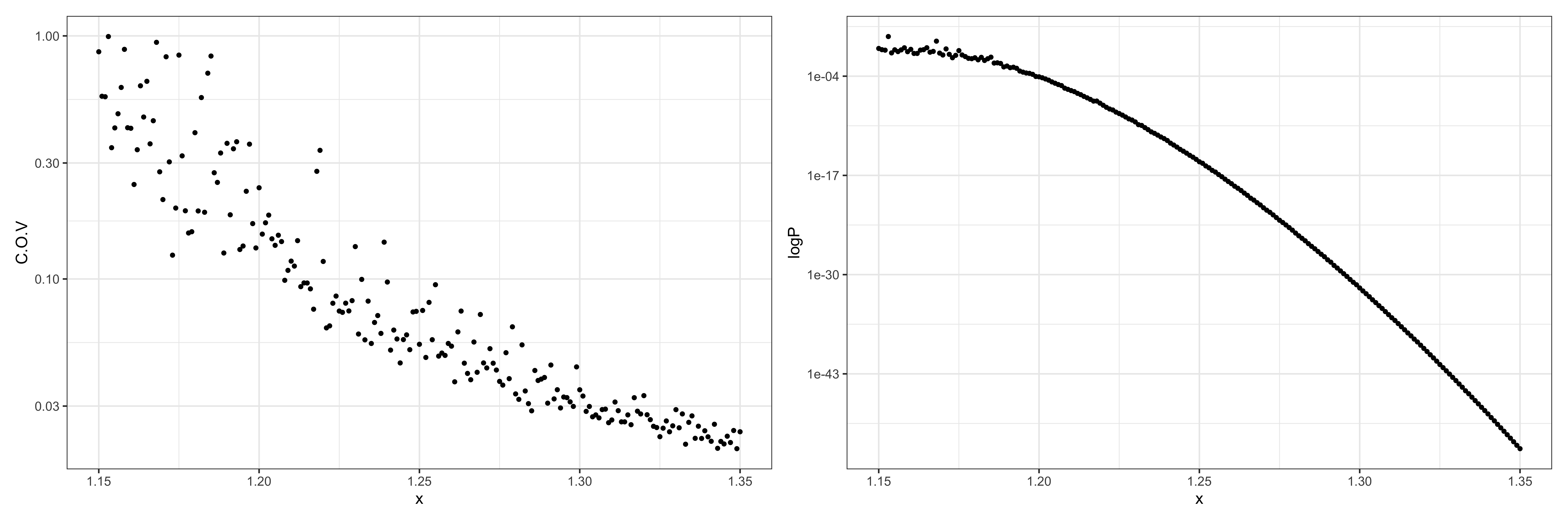
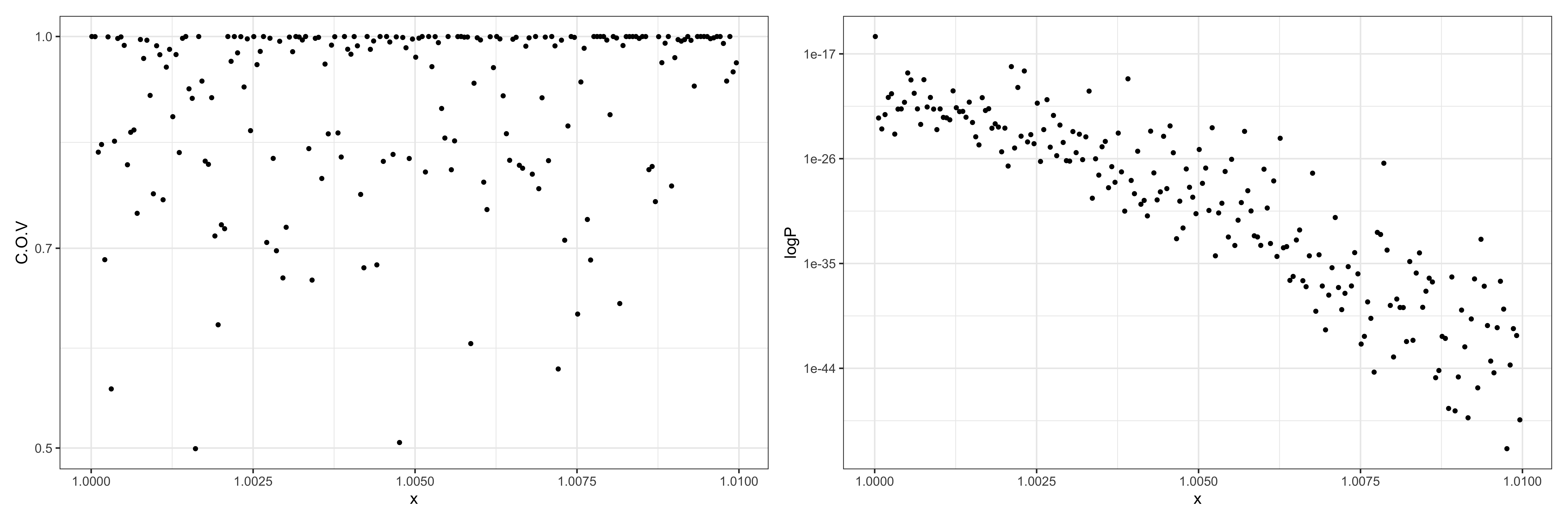
Based on 104superscript10410^{4} independent simulations and using the previously mentioned algorithm along with the R language, we carried out a series of simulation experiments. The left side of each graph shows the relationship between the coefficient of variation of sampled data F(1),…,F(N)superscript𝐹1…superscript𝐹𝑁F^{(1)},\ldots,F^{(N)} and xπ‘₯x. The right side of each graph depicts the relationship between the estimated values of ℙ​(Ξ»(n)>x)β„™subscriptπœ†π‘›π‘₯\mathbb{P}\left(\lambda_{(n)}>x\right) and xπ‘₯x on a logarithmic scale axis.

R code of the proposed algorithm can be found at https://github.com/S1yuW/Rare-event.

Refer to caption
Figure 1. 𝐇0subscript𝐇0{\bf H}_{0}: Ξ²=1𝛽1\beta=1, n=10𝑛10n=10, p1=103subscript𝑝1superscript103p_{1}=10^{3} and p2=109subscript𝑝2superscript109p_{2}=10^{9}.
Refer to caption
Figure 2. 𝐇1subscript𝐇1{\bf H}_{1}: Ξ²=10𝛽10\beta=10, n=10𝑛10n=10, p1=103subscript𝑝1superscript103p_{1}=10^{3} and p2=109subscript𝑝2superscript109p_{2}=10^{9}.
Refer to caption
Figure 3. 𝐇2subscript𝐇2{\bf H}_{2}: Ξ²=100𝛽100\beta=100, n=10𝑛10n=10, p1=103subscript𝑝1superscript103p_{1}=10^{3} and p2=109subscript𝑝2superscript109p_{2}=10^{9}.

Under 𝐇0subscript𝐇0{\bf H}_{0} and 𝐇1subscript𝐇1{\bf H}_{1}, the decreasing coefficient of variation with increasing xπ‘₯x means the stability and precision of the importance sample (IS) estimator. In the context of 𝐇0subscript𝐇0{\bf H}_{0}, the relatively smooth curve of the estimated values reflects the stability and consistency of the IS estimator. Specifically, when rare events are not exceedingly rare under 𝐇1subscript𝐇1{\bf H}_{1}, the coefficient of variation nearly approaches 1, leading to noticeable fluctuations in the IS estimator’s values curve. By contrast, under 𝐇0subscript𝐇0{\bf H}_{0}, the coefficient of variation remains relatively small, maintaining the smoothness of the curve. This emphasizes that the IS estimator under 𝐇1subscript𝐇1{\bf H}_{1} is more sensitive and exhibits stronger uncertainty compared to the IS estimator under 𝐇0subscript𝐇0{\bf H}_{0}. Furthermore, the IS estimator under 𝐇0subscript𝐇0{\bf H}_{0} demonstrates stronger consistency compared to the IS estimator under 𝐇1subscript𝐇1{\bf H}_{1}. Finally, under 𝐇2subscript𝐇2{\bf H}_{2}, the estimated values curve displays a general declining trend, but the overall instability in the IS estimator’s values emphasizes the differences between a weakly efficient IS estimator and a strongly efficient one.

4. Technical lemmas

Before the proof of Theorem 1, some lemmas needed are listed in Section 4. We will prove Theorem 1 in Sections 5. And the proofs of lemmas in the previous sections will be presented in the supplementary material.

We first present a basic inequality, borrowed from [11].

Lemma 1.

For Ξ±1>1/2subscript𝛼112\alpha_{1}>1/2 and 0<Ξ±2<1/20subscript𝛼2120<\alpha_{2}<1/2, we have

log⁑(1βˆ’z)β‰₯βˆ’zβˆ’Ξ±1​z2,Β if ​z∈(βˆ’1,1βˆ’12​α1);formulae-sequence1𝑧𝑧subscript𝛼1superscript𝑧2Β if 𝑧1112subscript𝛼1\displaystyle\log(1-z)\geq-z-\alpha_{1}z^{2},\quad\text{ if }z\in\left(-1,1-\frac{1}{2\alpha_{1}}\right);
log⁑(1+z)≀zβˆ’Ξ±2​z2,Β if ​z∈(βˆ’1,12​α2βˆ’1).formulae-sequence1𝑧𝑧subscript𝛼2superscript𝑧2Β if 𝑧112subscript𝛼21\displaystyle\log(1+z)\leq z-\alpha_{2}z^{2},\quad\text{ if }z\in\left(-1,\frac{1}{2\alpha_{2}}-1\right).

The following lemma provides some basic properties of the beta distributions. The first two results are clear and the third one is taken from [20].

Lemma 2.

Let X𝑋X be a Beta-distributed random variable with parameter aπ‘Ža and b,𝑏b, denoted by X∼Beta​(a,b),similar-to𝑋Betaπ‘Žπ‘X\sim{\rm Beta}(a,b), that equivalently means the density function of X𝑋X is

Γ​(a+b)Γ​(a)​Γ​(b)​xaβˆ’1​(1βˆ’x)bβˆ’1​10<x<1.Ξ“π‘Žπ‘Ξ“π‘ŽΞ“π‘superscriptπ‘₯π‘Ž1superscript1π‘₯𝑏1subscript10π‘₯1\frac{\Gamma(a+b)}{\Gamma(a)\Gamma(b)}x^{a-1}(1-x)^{b-1}1_{0<x<1}.

The following three assertions hold true.

  • (i)

    The kπ‘˜k-th moment of X𝑋X is

    𝔼​[Xk]=∏i=1ka+iβˆ’1a+b+iβˆ’1.𝔼delimited-[]superscriptπ‘‹π‘˜superscriptsubscriptproduct𝑖1π‘˜π‘Žπ‘–1π‘Žπ‘π‘–1\displaystyle\mathbb{E}\left[X^{k}\right]=\prod_{i=1}^{k}\frac{a+i-1}{a+b+i-1}.
  • (ii)

    The variance of X𝑋X and X2superscript𝑋2X^{2} are

    Var⁑[X]Var𝑋\displaystyle\operatorname{Var}[X] =a​b(a+b)2​(a+b+1),absentπ‘Žπ‘superscriptπ‘Žπ‘2π‘Žπ‘1\displaystyle=\frac{ab}{(a+b)^{2}(a+b+1)},
    Var⁑[X2]Varsuperscript𝑋2\displaystyle\operatorname{Var}\left[X^{2}\right] =a​(a+1)​(4​a​b​(a+b+3)+6​b2+b)(a+b)2​(a+b+1)2​(a+b+2)​(a+b+3).absentπ‘Žπ‘Ž14π‘Žπ‘π‘Žπ‘36superscript𝑏2𝑏superscriptπ‘Žπ‘2superscriptπ‘Žπ‘12π‘Žπ‘2π‘Žπ‘3\displaystyle=\frac{a(a+1)\left(4ab(a+b+3)+6b^{2}+b\right)}{(a+b)^{2}(a+b+1)^{2}(a+b+2)(a+b+3)}.
  • (iii)

    For any 0<Ξ΅<1/2,0πœ€120<\varepsilon<1/2,

    ℙ​(|Xβˆ’π”Όβ€‹[X]|>Ξ΅)≀4​exp⁑{βˆ’Ξ΅2128β‹…a3+b3a​b}.ℙ𝑋𝔼delimited-[]π‘‹πœ€4β‹…superscriptπœ€2128superscriptπ‘Ž3superscript𝑏3π‘Žπ‘\mathbb{P}(|X-\mathbb{E}[X]|>\varepsilon)\leq 4\exp\left\{-\frac{\varepsilon^{2}}{128}\cdot\frac{a^{3}+b^{3}}{ab}\right\}.

Now, we are going to state some lemmas on the asymptotic of ℙ​(Ξ»(n)>p1p​x).β„™subscriptπœ†π‘›subscript𝑝1𝑝π‘₯\mathbb{P}\left(\lambda_{(n)}>\frac{p_{1}}{p}x\right). To shorten the formula, set

(4.1) un​(x)=xr1,nβˆ’1​(1βˆ’x)r2,nβˆ’1subscript𝑒𝑛π‘₯superscriptπ‘₯subscriptπ‘Ÿ1𝑛1superscript1π‘₯subscriptπ‘Ÿ2𝑛1u_{n}(x)=x^{r_{1,n}-1}\left(1-x\right)^{r_{2,n}-1}

with ri,n=β​(piβˆ’n+1)/2subscriptπ‘Ÿπ‘–π‘›π›½subscript𝑝𝑖𝑛12r_{i,n}=\beta(p_{i}-n+1)/2 for i=1,2.𝑖12i=1,2. Throughout our analysis, we frequently use the factorization of the joint probability density function in (1.2) as below:

(4.2) d​Gnp1,p2=n​Anp1,p2β€‹βˆi=1nβˆ’1(xnβˆ’xi)β​un​(xn)​1{xn>xnβˆ’1}​d​xn​d​Gnβˆ’1p1βˆ’1,p2βˆ’1,dsuperscriptsubscript𝐺𝑛subscript𝑝1subscript𝑝2𝑛superscriptsubscript𝐴𝑛subscript𝑝1subscript𝑝2superscriptsubscriptproduct𝑖1𝑛1superscriptsubscriptπ‘₯𝑛subscriptπ‘₯𝑖𝛽subscript𝑒𝑛subscriptπ‘₯𝑛subscript1subscriptπ‘₯𝑛subscriptπ‘₯𝑛1dsubscriptπ‘₯𝑛dsuperscriptsubscript𝐺𝑛1subscript𝑝11subscript𝑝21\displaystyle\mathrm{d}G_{n}^{p_{1},p_{2}}=nA_{n}^{p_{1},p_{2}}\prod_{i=1}^{n-1}\left(x_{n}-x_{i}\right)^{\beta}u_{n}(x_{n})1_{\left\{x_{n}>x_{n-1}\right\}}\mathrm{d}x_{n}\mathrm{~{}d}G_{n-1}^{p_{1}-1,p_{2}-1},

where Anp1,p2superscriptsubscript𝐴𝑛subscript𝑝1subscript𝑝2A_{n}^{p_{1},p_{2}} is defined by

(4.3) Anp1,p2=Γ​(1+Ξ²2)​Γ​(β​p2)​Γ​(β​(pβˆ’1)2)Γ​(1+β​n2)​Γ​(β​p12)​Γ​(β​p22)​Γ​(β​(pβˆ’n)2).superscriptsubscript𝐴𝑛subscript𝑝1subscript𝑝2Ξ“1𝛽2Γ𝛽𝑝2Γ𝛽𝑝12Ξ“1𝛽𝑛2Γ𝛽subscript𝑝12Γ𝛽subscript𝑝22Γ𝛽𝑝𝑛2\displaystyle A_{n}^{p_{1},p_{2}}=\frac{\Gamma\left(1+\frac{\beta}{2}\right)\Gamma\left(\frac{\beta p}{2}\right)\Gamma\left(\frac{\beta(p-1)}{2}\right)}{\Gamma\left(1+\frac{\beta n}{2}\right)\Gamma\left(\frac{\beta p_{1}}{2}\right)\Gamma\left(\frac{\beta p_{2}}{2}\right)\Gamma\left(\frac{\beta(p-n)}{2}\right)}.

Here, Gnβˆ’1p1βˆ’1,p2βˆ’1superscriptsubscript𝐺𝑛1subscript𝑝11subscript𝑝21G_{n-1}^{p_{1}-1,p_{2}-1} represents the joint distribution of the order statistics of β𝛽\beta-Jacobi ensemble π’₯nβˆ’1​(p1βˆ’1,p2βˆ’1)subscriptπ’₯𝑛1subscript𝑝11subscript𝑝21\mathcal{J}_{n-1}\left(p_{1}-1,p_{2}-1\right).

Observing the terms in (4.2) one by one, we give first the asymptotical expression of log⁑Anp1,p2superscriptsubscript𝐴𝑛subscript𝑝1subscript𝑝2\log A_{n}^{p_{1},p_{2}} under the condition A, where A is given as

𝐀:limnβ†’βˆžnp1=0,limnβ†’βˆžp1p2=Οƒβˆˆ[0,∞)Β andΒ Ξ²n>>1.{\bf A}:\quad\quad\quad\lim_{n\to\infty}\frac{n}{p_{1}}=0,\quad\lim_{n\to\infty}\frac{p_{1}}{p_{2}}=\sigma\in[0,\infty)\quad\text{ and }\quad\beta n\!>\!>1.
Lemma 3.

Let Anp1,p2superscriptsubscript𝐴𝑛subscript𝑝1subscript𝑝2A_{n}^{p_{1},p_{2}} be defined by (4.3). Under the assumption A, we have

log⁑Anp1,p2=β​p12​log⁑pp1+β​p22​log⁑pp2+β​(nβˆ’1)2​log⁑pn+12​log⁑(β​p1)+12​β​n+o​(β​n).superscriptsubscript𝐴𝑛subscript𝑝1subscript𝑝2𝛽subscript𝑝12𝑝subscript𝑝1𝛽subscript𝑝22𝑝subscript𝑝2𝛽𝑛12𝑝𝑛12𝛽subscript𝑝112π›½π‘›π‘œπ›½π‘›\log A_{n}^{p_{1},p_{2}}=\frac{\beta p_{1}}{2}\log\frac{p}{p_{1}}+\frac{\beta p_{2}}{2}\log\frac{p}{p_{2}}+\frac{\beta(n-1)}{2}\log\frac{p}{n}+\frac{1}{2}\log(\beta p_{1})+\frac{1}{2}\beta n+o(\beta n).
Proof.

By definition,

log⁑Anp1,p2=superscriptsubscript𝐴𝑛subscript𝑝1subscript𝑝2absent\displaystyle\log A_{n}^{p_{1},p_{2}}= log⁑Γ​(1+Ξ²2)+log⁑Γ​(β​p2)+log⁑Γ​(β​(pβˆ’1)2)Ξ“1𝛽2Γ𝛽𝑝2Γ𝛽𝑝12\displaystyle\log\Gamma\left(1+\frac{\beta}{2}\right)+\log\Gamma\left(\frac{\beta p}{2}\right)+\log\Gamma\left(\frac{\beta(p-1)}{2}\right)
βˆ’log⁑Γ​(1+β​n2)βˆ’log⁑Γ​(β​p12)βˆ’log⁑Γ​(β​p22)βˆ’log⁑Γ​(β​(pβˆ’n)2).Ξ“1𝛽𝑛2Γ𝛽subscript𝑝12Γ𝛽subscript𝑝22Γ𝛽𝑝𝑛2\displaystyle-\log\Gamma\left(1+\frac{\beta n}{2}\right)-\log\Gamma\left(\frac{\beta p_{1}}{2}\right)-\log\Gamma\left(\frac{\beta p_{2}}{2}\right)-\log\Gamma\left(\frac{\beta(p-n)}{2}\right).

The Stirling formula says that

log⁑Γ​(x)=(xβˆ’12)​log⁑xβˆ’x+12​log⁑(2​π)+o​(1)Ξ“π‘₯π‘₯12π‘₯π‘₯122πœ‹π‘œ1\log\Gamma(x)=\left(x-\frac{1}{2}\right)\log x-x+\frac{1}{2}\log\left(2\pi\right)+o(1)

for sufficiently large xπ‘₯x. Then, by combining alike terms, we see that

log⁑Anp1,p2=superscriptsubscript𝐴𝑛subscript𝑝1subscript𝑝2absent\displaystyle\log A_{n}^{p_{1},p_{2}}= log⁑Γ​(1+Ξ²2)βˆ’Ξ²2​log⁑β2+β​p12​log⁑pp1+β​p22​log⁑pp2Ξ“1𝛽2𝛽2𝛽2𝛽subscript𝑝12𝑝subscript𝑝1𝛽subscript𝑝22𝑝subscript𝑝2\displaystyle\log\Gamma\left(1+\frac{\beta}{2}\right)-\frac{\beta}{2}\log\frac{\beta}{2}+\frac{\beta p_{1}}{2}\log\frac{p}{p_{1}}+\frac{\beta p_{2}}{2}\log\frac{p}{p_{2}}
+(β​(pβˆ’n)2βˆ’12)​log⁑pβˆ’1pβˆ’n+β​(nβˆ’1)2​log⁑β​(pβˆ’1)2+β​n𝛽𝑝𝑛212𝑝1𝑝𝑛𝛽𝑛12𝛽𝑝12𝛽𝑛\displaystyle+\left(\frac{\beta(p-n)}{2}-\frac{1}{2}\right)\log\frac{p-1}{p-n}+\frac{\beta(n-1)}{2}\log\frac{\beta(p-1)}{2+\beta n}
(4.4) +12​log⁑β​p12βˆ’Ξ²+12​log⁑n2βˆ’12​log⁑(2​π)+o​(1).12𝛽subscript𝑝12𝛽12𝑛2122πœ‹π‘œ1\displaystyle+\frac{1}{2}\log\frac{\beta p_{1}}{2}-\frac{\beta+1}{2}\log\frac{n}{2}-\frac{1}{2}\log\left(2\pi\right)+o(1).

Since log⁑Γ​(1+Ξ²2)βˆ’Ξ²2​log⁑β2Ξ“1𝛽2𝛽2𝛽2\log\Gamma\left(1+\frac{\beta}{2}\right)-\frac{\beta}{2}\log\frac{\beta}{2} is either O​(Ξ²)𝑂𝛽O(\beta) for β𝛽\beta large enough or bounded for finite β𝛽\beta and

(β​(pβˆ’n)2βˆ’12)​log⁑pβˆ’1pβˆ’n=12​β​n+o​(β​n),𝛽𝑝𝑛212𝑝1𝑝𝑛12π›½π‘›π‘œπ›½π‘›\left(\frac{\beta(p-n)}{2}-\frac{1}{2}\right)\log\frac{p-1}{p-n}=\frac{1}{2}\beta n+o(\beta n),

it comes

log⁑Anp1,p2=β​p12​log⁑pp1+β​p22​log⁑pp2+β​(nβˆ’1)2​log⁑pn+12​log⁑β​p1+12​β​n+o​(β​n).superscriptsubscript𝐴𝑛subscript𝑝1subscript𝑝2𝛽subscript𝑝12𝑝subscript𝑝1𝛽subscript𝑝22𝑝subscript𝑝2𝛽𝑛12𝑝𝑛12𝛽subscript𝑝112π›½π‘›π‘œπ›½π‘›\displaystyle\log A_{n}^{p_{1},p_{2}}=\frac{\beta p_{1}}{2}\log\frac{p}{p_{1}}+\frac{\beta p_{2}}{2}\log\frac{p}{p_{2}}+\frac{\beta(n-1)}{2}\log\frac{p}{n}+\frac{1}{2}\log\beta p_{1}+\frac{1}{2}\beta n+o(\beta n).

∎

Now, we state a lemma on integrals of some strictly convex function.

Lemma 4.

Suppose 0≀m<a<M≀10π‘šπ‘Žπ‘€10\leq m<a<M\leq 1 and kβ‰₯0π‘˜0k\geq 0 and b,c>1.𝑏𝑐1b,c>1. Let

ω​(t)=βˆ’k​tβˆ’(bβˆ’1)​ln⁑tβˆ’(cβˆ’1)​ln⁑(1βˆ’t),0<t<1.formulae-sequenceπœ”π‘‘π‘˜π‘‘π‘1𝑑𝑐11𝑑0𝑑1\omega(t)=-k\,t-(b-1)\ln t-(c-1)\ln(1-t),\quad 0<t<1.
  • (i)

    If ω′​(a)>0,superscriptπœ”β€²π‘Ž0\omega^{\prime}(a)>0, then we have

    ∫aMeβˆ’Ο‰β€‹(t)​dt≀eβˆ’k​a​abβˆ’1​(1βˆ’a)cβˆ’1ω′​(a)superscriptsubscriptπ‘Žπ‘€superscriptπ‘’πœ”π‘‘differential-d𝑑superscriptπ‘’π‘˜π‘Žsuperscriptπ‘Žπ‘1superscript1π‘Žπ‘1superscriptπœ”β€²π‘Ž\displaystyle\int_{a}^{M}e^{-\omega(t)}\mathrm{~{}d}t\leq\frac{e^{-k\,a}a^{b-1}(1-a)^{c-1}}{\omega^{\prime}(a)}

    and

    ∫aMeβˆ’Ο‰β€‹(t)​dtβ‰₯superscriptsubscriptπ‘Žπ‘€superscriptπ‘’πœ”π‘‘differential-d𝑑absent\displaystyle\int_{a}^{M}e^{-\omega(t)}\mathrm{~{}d}t\geq eβˆ’k​a​abβˆ’1​(1βˆ’a)cβˆ’1ω′​(M)​(1βˆ’exp⁑{βˆ’(Mβˆ’a)​ω′​(a)}).superscriptπ‘’π‘˜π‘Žsuperscriptπ‘Žπ‘1superscript1π‘Žπ‘1superscriptπœ”β€²π‘€1π‘€π‘Žsuperscriptπœ”β€²π‘Ž\displaystyle\frac{e^{-k\,a}a^{b-1}(1-a)^{c-1}}{\omega^{\prime}(M)}\left(1-\exp\left\{-(M-a)\omega^{\prime}(a)\right\}\right).
  • (ii)

    By contrast, it holds that

    ∫maeβˆ’Ο‰β€‹(t)​dt≀eβˆ’k​a​abβˆ’1​(1βˆ’a)cβˆ’1βˆ’Ο‰β€²β€‹(a)superscriptsubscriptπ‘šπ‘Žsuperscriptπ‘’πœ”π‘‘differential-d𝑑superscriptπ‘’π‘˜π‘Žsuperscriptπ‘Žπ‘1superscript1π‘Žπ‘1superscriptπœ”β€²π‘Ž\displaystyle\int_{m}^{a}e^{-\omega(t)}\mathrm{~{}d}t\leq\frac{e^{-k\,a}a^{b-1}(1-a)^{c-1}}{-\omega^{\prime}(a)}

    and

    ∫maeβˆ’Ο‰β€‹(t)​dtβ‰₯eβˆ’k​a​abβˆ’1​(1βˆ’a)cβˆ’1βˆ’Ο‰β€²β€‹(m)​(1βˆ’exp⁑{(aβˆ’m)​ω′​(a)})superscriptsubscriptπ‘šπ‘Žsuperscriptπ‘’πœ”π‘‘differential-d𝑑superscriptπ‘’π‘˜π‘Žsuperscriptπ‘Žπ‘1superscript1π‘Žπ‘1superscriptπœ”β€²π‘š1π‘Žπ‘šsuperscriptπœ”β€²π‘Ž\displaystyle\int_{m}^{a}e^{-\omega(t)}\mathrm{~{}d}t\geq\frac{e^{-k\,a}a^{b-1}(1-a)^{c-1}}{-\omega^{\prime}(m)}\left(1-\exp\left\{(a-m)\omega^{\prime}(a)\right\}\right)

    for aπ‘Ža when ω′​(a)<0.superscriptπœ”β€²π‘Ž0\omega^{\prime}(a)<0.

Next, based on Lemma 4, we provide accurate estimates on integrals of un​(x)=xr1,nβˆ’1​(1βˆ’x)r2,nβˆ’1.subscript𝑒𝑛π‘₯superscriptπ‘₯subscriptπ‘Ÿ1𝑛1superscript1π‘₯subscriptπ‘Ÿ2𝑛1u_{n}(x)=x^{r_{1,n}-1}(1-x)^{r_{2,n}-1}.

Lemma 5.

Suppose that n<<p1<<p2.much-less-than𝑛subscript𝑝1much-less-thansubscript𝑝2n<\!<\!p_{1}<\!<\!p_{2}.

  • (i)

    Given x>1.π‘₯1x>1. For zn>0subscript𝑧𝑛0z_{n}>0 with np1<<zn<<1much-less-than𝑛subscript𝑝1subscript𝑧𝑛much-less-than1\frac{n}{p_{1}}<\!<\!z_{n}<\!<\!1 and ΞΊn=o​(β​p),subscriptπœ…π‘›π‘œπ›½π‘\kappa_{n}=o(\beta p), we have

    ∫p1​xpp1​(x+zn)pexp⁑{ΞΊn​(yβˆ’p1​xp)}​un​(y)​dy=2​x(xβˆ’1)​β​p​un​(p1​xp)​(1+o​(1)).superscriptsubscriptsubscript𝑝1π‘₯𝑝subscript𝑝1π‘₯subscript𝑧𝑛𝑝subscriptπœ…π‘›π‘¦subscript𝑝1π‘₯𝑝subscript𝑒𝑛𝑦differential-d𝑦2π‘₯π‘₯1𝛽𝑝subscript𝑒𝑛subscript𝑝1π‘₯𝑝1π‘œ1\displaystyle\int_{\frac{p_{1}x}{p}}^{\frac{p_{1}(x+z_{n})}{p}}\exp\left\{\kappa_{n}\left(y-\frac{p_{1}x}{p}\right)\right\}u_{n}\left(y\right)\mathrm{~{}d}y=\frac{2x}{(x-1)\beta p}u_{n}\left(\frac{p_{1}x}{p}\right)(1+o(1)).
  • (ii)

    Given zn>0subscript𝑧𝑛0z_{n}>0 with np1<<zn≀M<∞much-less-than𝑛subscript𝑝1subscript𝑧𝑛𝑀\frac{n}{p_{1}}<\!<z_{n}\leq M<\infty and let l𝑙l be a positive integer. Supposing that dn=O​(β​n)subscript𝑑𝑛𝑂𝛽𝑛d_{n}=O(\beta n) and the sequence ΞΊnsubscriptπœ…π‘›\kappa_{n} satisfying

    limnβ†’βˆž(βˆ’ΞΊnβ​p​zn+l2​(1+zn))=c>0,subscript→𝑛subscriptπœ…π‘›π›½π‘subscript𝑧𝑛𝑙21subscript𝑧𝑛𝑐0\lim_{n\to\infty}\left(-\frac{\kappa_{n}}{\beta pz_{n}}+\frac{l}{2(1+z_{n})}\right)=c>0,

    we claim that

    ∫p1p​(1+zn)1exp⁑{ΞΊn​(yβˆ’p1​(1+zn)p)}​unl​(y)​ydn​dysuperscriptsubscriptsubscript𝑝1𝑝1subscript𝑧𝑛1subscriptπœ…π‘›π‘¦subscript𝑝11subscript𝑧𝑛𝑝superscriptsubscript𝑒𝑛𝑙𝑦superscript𝑦subscript𝑑𝑛differential-d𝑦\displaystyle\quad\int_{\frac{p_{1}}{p}\left(1+z_{n}\right)}^{1}\exp\left\{\kappa_{n}\left(y-\frac{p_{1}(1+z_{n})}{p}\right)\right\}u_{n}^{l}(y)y^{d_{n}}\mathrm{~{}d}y
    ≀1c​β​p​zn​unl​(p1​(1+zn)p)​(p1​(1+zn)p)dn​(1+o​(1)).absent1𝑐𝛽𝑝subscript𝑧𝑛superscriptsubscript𝑒𝑛𝑙subscript𝑝11subscript𝑧𝑛𝑝superscriptsubscript𝑝11subscript𝑧𝑛𝑝subscript𝑑𝑛1π‘œ1\displaystyle\leq\frac{1}{c\,\beta pz_{n}}u_{n}^{l}\left(\frac{p_{1}(1+z_{n})}{p}\right)\left(\frac{p_{1}(1+z_{n})}{p}\right)^{d_{n}}(1+o(1)).
  • (iii)

    Given zn>0subscript𝑧𝑛0z_{n}>0 with np1<<zn<<1much-less-than𝑛subscript𝑝1subscript𝑧𝑛much-less-than1\frac{n}{p_{1}}<\!<z_{n}<\!<1 and ΞΊn=o​(β​p),subscriptπœ…π‘›π‘œπ›½π‘\kappa_{n}=o(\beta p), we have

    ∫0p1​(1βˆ’zn)pexp⁑{ΞΊn​(yβˆ’p1​(1βˆ’zn)p)}​un​(y)​dy≀2β​p​zn​un​(p1​(1βˆ’zn)p)​(1+o​(1)).superscriptsubscript0subscript𝑝11subscript𝑧𝑛𝑝subscriptπœ…π‘›π‘¦subscript𝑝11subscript𝑧𝑛𝑝subscript𝑒𝑛𝑦differential-d𝑦2𝛽𝑝subscript𝑧𝑛subscript𝑒𝑛subscript𝑝11subscript𝑧𝑛𝑝1π‘œ1\displaystyle\int_{0}^{\frac{p_{1}(1-z_{n})}{p}}\exp\left\{\kappa_{n}\left(y-\frac{p_{1}(1-z_{n})}{p}\right)\right\}u_{n}(y)\mathrm{~{}d}y\leq\frac{2}{\beta pz_{n}}u_{n}\left(\frac{p_{1}(1-z_{n})}{p}\right)(1+o(1)).

In order to treat the terms in the expression (4.2), it remains to investigate the interaction ∏i=1nβˆ’1|xnβˆ’xi|,superscriptsubscriptproduct𝑖1𝑛1subscriptπ‘₯𝑛subscriptπ‘₯𝑖\prod_{i=1}^{n-1}|x_{n}-x_{i}|, which produces the main difficulties. For that aim, we introduce a particular set En,subscript𝐸𝑛E_{n}, defined as

(4.5) En={(x1,β‹―,xn)βˆˆΞ”n|p1p​(1βˆ’Ξ΄n)<x1,xnβˆ’1<p1p​(1+Ξ΄n),p1p​x<xn<p1p​(x+Ξ΄n)}.subscript𝐸𝑛conditional-setsubscriptπ‘₯1β‹―subscriptπ‘₯𝑛subscriptΔ𝑛formulae-sequencesubscript𝑝1𝑝1subscript𝛿𝑛subscriptπ‘₯1formulae-sequencesubscriptπ‘₯𝑛1subscript𝑝1𝑝1subscript𝛿𝑛subscript𝑝1𝑝π‘₯subscriptπ‘₯𝑛subscript𝑝1𝑝π‘₯subscript𝛿𝑛\displaystyle E_{n}=\left\{(x_{1},\cdots,x_{n})\in\Delta_{n}\left|\frac{p_{1}}{p}(1-\delta_{n})<x_{1},x_{n-1}<\frac{p_{1}}{p}(1+\delta_{n}),\frac{p_{1}}{p}x<x_{n}<\frac{p_{1}}{p}\left(x+\delta_{n}\right)\right.\right\}.

Here, Ξ”n:={(x1,β‹―,xn)∈[0,1]n:x1≀x2≀⋯≀xn}.assignsubscriptΔ𝑛conditional-setsubscriptπ‘₯1β‹―subscriptπ‘₯𝑛superscript01𝑛subscriptπ‘₯1subscriptπ‘₯2β‹―subscriptπ‘₯𝑛\Delta_{n}:=\{(x_{1},\cdots,x_{n})\in[0,1]^{n}:x_{1}\leq x_{2}\leq\cdots\leq x_{n}\}.

Lemma 6.

Given x>1π‘₯1x>1 and 0<Ξ΄n<<10subscript𝛿𝑛much-less-than10<\delta_{n}<\!<\!1 and let Ensubscript𝐸𝑛E_{n} be defined as above. Set

Ξ±2=12βˆ’Ξ΄nxβˆ’1,Ξ±1=12+Ξ΄nxβˆ’1andxΒ―i=p​xiβˆ’p1p1​(xβˆ’1).formulae-sequencesubscript𝛼212subscript𝛿𝑛π‘₯1formulae-sequencesubscript𝛼112subscript𝛿𝑛π‘₯1andsubscriptΒ―π‘₯𝑖𝑝subscriptπ‘₯𝑖subscript𝑝1subscript𝑝1π‘₯1\alpha_{2}=\frac{1}{2}-\frac{\delta_{n}}{x-1},\quad\alpha_{1}=\frac{1}{2}+\frac{\delta_{n}}{x-1}\quad\text{and}\quad\bar{x}_{i}=\frac{px_{i}-p_{1}}{p_{1}(x-1)}.

For all (x1,…,xn)∈En,subscriptπ‘₯1…subscriptπ‘₯𝑛subscript𝐸𝑛(x_{1},\ldots,x_{n})\in E_{n}, the interaction ∏i=1nβˆ’1(xnβˆ’xi)superscriptsubscriptproduct𝑖1𝑛1subscriptπ‘₯𝑛subscriptπ‘₯𝑖\prod_{i=1}^{n-1}\left(x_{n}-x_{i}\right) has lower and upper bounds as follows

∏i=1nβˆ’1(xnβˆ’xi)superscriptsubscriptproduct𝑖1𝑛1subscriptπ‘₯𝑛subscriptπ‘₯𝑖\displaystyle\prod_{i=1}^{n-1}\left(x_{n}-x_{i}\right) ≀(p1​(xβˆ’1)p)nβˆ’1​exp⁑{(n+o​(n))​p​xnβˆ’p1​xp1​(xβˆ’1)βˆ’βˆ‘i=1nβˆ’1xΒ―iβˆ’Ξ±2β€‹βˆ‘i=1nβˆ’1xΒ―i2};absentsuperscriptsubscript𝑝1π‘₯1𝑝𝑛1π‘›π‘œπ‘›π‘subscriptπ‘₯𝑛subscript𝑝1π‘₯subscript𝑝1π‘₯1superscriptsubscript𝑖1𝑛1subscriptΒ―π‘₯𝑖subscript𝛼2superscriptsubscript𝑖1𝑛1superscriptsubscriptΒ―π‘₯𝑖2\displaystyle\leq\left(\frac{p_{1}(x-1)}{p}\right)^{n-1}\exp\left\{(n+o(n))\frac{px_{n}-p_{1}x}{p_{1}(x-1)}-\sum_{i=1}^{n-1}\bar{x}_{i}-\alpha_{2}\sum_{i=1}^{n-1}\bar{x}_{i}^{2}\right\};
∏i=1nβˆ’1(xnβˆ’xi)superscriptsubscriptproduct𝑖1𝑛1subscriptπ‘₯𝑛subscriptπ‘₯𝑖\displaystyle\prod_{i=1}^{n-1}\left(x_{n}-x_{i}\right) β‰₯(p1​(xβˆ’1)p)nβˆ’1​exp⁑{βˆ’βˆ‘i=1nβˆ’1xΒ―iβˆ’Ξ±1β€‹βˆ‘i=1nβˆ’1xΒ―i2}.absentsuperscriptsubscript𝑝1π‘₯1𝑝𝑛1superscriptsubscript𝑖1𝑛1subscriptΒ―π‘₯𝑖subscript𝛼1superscriptsubscript𝑖1𝑛1superscriptsubscriptΒ―π‘₯𝑖2\displaystyle\geq\left(\frac{p_{1}(x-1)}{p}\right)^{n-1}\exp\left\{-\sum_{i=1}^{n-1}\bar{x}_{i}-\alpha_{1}\sum_{i=1}^{n-1}\bar{x}_{i}^{2}\right\}.

Lemma 6 guides us to work on the following two lemmas, whose proofs are relatively long and are postponed to the last section.

Lemma 7.

Let (Ξ»1,Ξ»2,β‹―,Ξ»n)subscriptπœ†1subscriptπœ†2β‹―subscriptπœ†π‘›\left(\lambda_{1},\lambda_{2},\cdots,\lambda_{n}\right) be the β𝛽\beta-Jacobi ensemble π’₯n​(p1,p2)subscriptπ’₯𝑛subscript𝑝1subscript𝑝2\mathcal{J}_{n}(p_{1},p_{2}) with density function (1.1). For n𝑛n large enough, we have

𝔼​[βˆ‘i=1n(p​λiβˆ’p1p1)]=O​(n2p);𝔼delimited-[]superscriptsubscript𝑖1𝑛𝑝subscriptπœ†π‘–subscript𝑝1subscript𝑝1𝑂superscript𝑛2𝑝\displaystyle\mathbb{E}\left[\sum_{i=1}^{n}\left(\frac{p\lambda_{i}-p_{1}}{p_{1}}\right)\right]=O\left(\frac{n^{2}}{p}\right);
𝔼​[βˆ‘i=1n(p​λiβˆ’p1p1)2]=n2p1+O​(n2p+nβ​p1+n2p12).𝔼delimited-[]superscriptsubscript𝑖1𝑛superscript𝑝subscriptπœ†π‘–subscript𝑝1subscript𝑝12superscript𝑛2subscript𝑝1𝑂superscript𝑛2𝑝𝑛𝛽subscript𝑝1superscript𝑛2superscriptsubscript𝑝12\displaystyle\mathbb{E}\left[\sum_{i=1}^{n}\left(\frac{p\lambda_{i}-p_{1}}{p_{1}}\right)^{2}\right]=\frac{n^{2}}{p_{1}}+O\left(\frac{n^{2}}{p}+\frac{n}{\beta p_{1}}+\frac{n^{2}}{p_{1}^{2}}\right).
Lemma 8.

Let (Ξ»1,Ξ»2,β‹―,Ξ»n)subscriptπœ†1subscriptπœ†2β‹―subscriptπœ†π‘›\left(\lambda_{1},\lambda_{2},\cdots,\lambda_{n}\right) be the β𝛽\beta-Jacobi ensemble π’₯n​(p1,p2)subscriptπ’₯𝑛subscript𝑝1subscript𝑝2\mathcal{J}_{n}(p_{1},p_{2}) with density function (1.1) and suppose that β​n​p12β‰ͺp2,nβ‰ͺp1formulae-sequencemuch-less-than𝛽𝑛superscriptsubscript𝑝12subscript𝑝2much-less-than𝑛subscript𝑝1\beta np_{1}^{2}\ll p_{2},\;n\ll p_{1} and (β​n)3β‰ͺ(β​p1)2.much-less-thansuperscript𝛽𝑛3superscript𝛽subscript𝑝12(\beta n)^{3}\ll(\beta p_{1})^{2}. We have the following three statements.

  1. (1)

    Given a positive sequence Ξ΄nsubscript𝛿𝑛\delta_{n} with np1β‰ͺΞ΄nβ‰ͺ1much-less-than𝑛subscript𝑝1subscript𝛿𝑛much-less-than1\sqrt{\frac{n}{p_{1}}}\ll\delta_{n}\ll 1 and Ξ±=O​(Ξ²Ξ΄n).𝛼𝑂𝛽subscript𝛿𝑛\alpha=O\left(\frac{\beta}{\delta_{n}}\right). It holds that

    (4.6) limnβ†’βˆžπ”Όβ€‹exp⁑{βˆ’Ξ±β€‹βˆ‘i=1n(p​λiβˆ’p1p1)}=1.subscript→𝑛𝔼𝛼superscriptsubscript𝑖1𝑛𝑝subscriptπœ†π‘–subscript𝑝1subscript𝑝11\displaystyle\lim_{n\rightarrow\infty}\mathbb{E}\exp\left\{-\alpha\sum_{i=1}^{n}\left(\frac{p\lambda_{i}-p_{1}}{p_{1}}\right)\right\}=1.
  2. (2)

    For the case when Ξ·1=O​(Ξ²)subscriptπœ‚1𝑂𝛽\eta_{1}=O(\beta) and Ξ·2=O​(Ξ²),subscriptπœ‚2𝑂𝛽\eta_{2}=O(\beta), we have that

    (4.7) limnβ†’βˆžπ”Όβ€‹[exp⁑{βˆ’Ξ·1β€‹βˆ‘i=1n(p​λiβˆ’p1p1)βˆ’Ξ·2β€‹βˆ‘i=1n(p​λiβˆ’p1p1)2+Ξ·2​n2p1}]=1.subscript→𝑛𝔼delimited-[]subscriptπœ‚1superscriptsubscript𝑖1𝑛𝑝subscriptπœ†π‘–subscript𝑝1subscript𝑝1subscriptπœ‚2superscriptsubscript𝑖1𝑛superscript𝑝subscriptπœ†π‘–subscript𝑝1subscript𝑝12subscriptπœ‚2superscript𝑛2subscript𝑝11\displaystyle\lim_{n\rightarrow\infty}\mathbb{E}\left[\exp\left\{-\eta_{1}\sum_{i=1}^{n}\left(\frac{p\lambda_{i}-p_{1}}{p_{1}}\right)-\eta_{2}\sum_{i=1}^{n}\left(\frac{p\lambda_{i}-p_{1}}{p_{1}}\right)^{2}+\frac{\eta_{2}n^{2}}{p_{1}}\right\}\right]=1.
  3. (3)

    Given a positive sequence Ξ΄nsubscript𝛿𝑛\delta_{n} satisfying n/p1β‰ͺΞ΄nβ‰ͺ1much-less-than𝑛subscript𝑝1subscript𝛿𝑛much-less-than1\sqrt{n/p_{1}}\ll\delta_{n}\ll 1 and 0<Ξ·1=O​(Ξ²),0<Ξ·2=O​(Ξ²).formulae-sequence0subscriptπœ‚1𝑂𝛽0subscriptπœ‚2𝑂𝛽0<\eta_{1}=O(\beta),0<\eta_{2}=O(\beta). It holds that

    𝔼​[exp⁑{βˆ’Ξ·1β€‹βˆ‘i=1n(p​λiβˆ’p1p1)βˆ’Ξ·2β€‹βˆ‘i=1n(p​λiβˆ’p1p1)2}β€‹πŸ{Ξ»(1)>p1p​(1βˆ’Ξ΄n),Ξ»(n)<p1p​(1+Ξ΄n)}]𝔼delimited-[]subscriptπœ‚1superscriptsubscript𝑖1𝑛𝑝subscriptπœ†π‘–subscript𝑝1subscript𝑝1subscriptπœ‚2superscriptsubscript𝑖1𝑛superscript𝑝subscriptπœ†π‘–subscript𝑝1subscript𝑝12subscript1formulae-sequencesubscriptπœ†1subscript𝑝1𝑝1subscript𝛿𝑛subscriptπœ†π‘›subscript𝑝1𝑝1subscript𝛿𝑛\displaystyle\mathbb{E}\left[\exp\left\{-\eta_{1}\sum_{i=1}^{n}\left(\frac{p\lambda_{i}-p_{1}}{p_{1}}\right)-\eta_{2}\sum_{i=1}^{n}\left(\frac{p\lambda_{i}-p_{1}}{p_{1}}\right)^{2}\right\}\mathbf{1}_{\left\{\lambda_{(1)}>\frac{p_{1}}{p}(1-\delta_{n}),\lambda_{(n)}<\frac{p_{1}}{p}(1+\delta_{n})\right\}}\right]
    (4.8) β‰₯\displaystyle\geq exp⁑{βˆ’Ξ·2​n2p1+o​(1)}subscriptπœ‚2superscript𝑛2subscript𝑝1π‘œ1\displaystyle\exp\left\{-\frac{\eta_{2}n^{2}}{p_{1}}+o\left(1\right)\right\}

    for n𝑛n large enough.

5. Proof of Theorem 1

To ease notations, we use 𝔼𝔼\mathbb{E} and 𝔼Lsuperscript𝔼𝐿\mathbb{E}^{L} to refer to the expectations with respect to Gnp1,p2superscriptsubscript𝐺𝑛subscript𝑝1subscript𝑝2G_{n}^{p_{1},p_{2}} and Lnp1,p2,superscriptsubscript𝐿𝑛subscript𝑝1subscript𝑝2L_{n}^{p_{1},p_{2}}, and use G𝐺G and L𝐿L for corresponding measures, respectively. Recall that the IS estimator

Fn=n​Anp1,p2β€‹βˆi=1nβˆ’1(Ξ»(n)βˆ’Ξ»(i))β​un​(Ξ»(n))​hβˆ’1​(Ξ»(n))β€‹πŸ{Ξ»(n)>p1​x/p},subscript𝐹𝑛𝑛superscriptsubscript𝐴𝑛subscript𝑝1subscript𝑝2superscriptsubscriptproduct𝑖1𝑛1superscriptsubscriptπœ†π‘›subscriptπœ†π‘–π›½subscript𝑒𝑛subscriptπœ†π‘›superscriptβ„Ž1subscriptπœ†π‘›subscript1subscriptπœ†π‘›subscript𝑝1π‘₯𝑝\displaystyle F_{n}=nA_{n}^{p_{1},p_{2}}\prod_{i=1}^{n-1}\left(\lambda_{(n)}-\lambda_{(i)}\right)^{\beta}u_{n}\left(\lambda_{(n)}\right)h^{-1}(\lambda_{(n)})\mathbf{1}_{\left\{\lambda_{(n)}>p_{1}x/p\right\}},

where the function hβ„Žh is given by

h​(y):=r1βˆ’eβˆ’r​(1βˆ’p1​x/p)​eβˆ’r​(yβˆ’(p1​x/p)∨λ(nβˆ’1))β€‹πŸ{(p1​x/p)∨λ(nβˆ’1)<y<1}assignβ„Žπ‘¦π‘Ÿ1superscriptπ‘’π‘Ÿ1subscript𝑝1π‘₯𝑝superscriptπ‘’π‘Ÿπ‘¦subscript𝑝1π‘₯𝑝subscriptπœ†π‘›1subscript1subscript𝑝1π‘₯𝑝subscriptπœ†π‘›1𝑦1h\left(y\right):=\frac{r}{1-e^{-r(1-p_{1}x/p)}}e^{-r\left(y-\left(p_{1}x/p\right)\vee\lambda_{(n-1)}\right)}\mathbf{1}_{\{\left(p_{1}x/p\right)\vee\lambda_{(n-1)}<y<1\}}

with rate r=β​p​(xβˆ’1)2​x.π‘Ÿπ›½π‘π‘₯12π‘₯r=\frac{\beta p(x-1)}{2x}. We first prove the result when H0 holds.

5.1. Proof of the third assertions of Theorem 1 when H0 is true.

For any Aβˆˆβ„¬n,𝐴superscriptℬ𝑛A\in\mathcal{B}^{n}, we know

|Lnp1,p2​(A)βˆ’β„™β€‹(A​|Ξ»(n)>​p1p​x)|=superscriptsubscript𝐿𝑛subscript𝑝1subscript𝑝2𝐴ℙ𝐴ketsubscriptπœ†π‘›subscript𝑝1𝑝π‘₯absent\displaystyle\left|L_{n}^{p_{1},p_{2}}(A)-\mathbb{P}\left(A\left|\lambda_{(n)}>\frac{p_{1}}{p}x\right.\right)\right|= |∫A1βˆ’Fnℙ​(Ξ»(n)>p1p​x)​d​Lnp1,p2|subscript𝐴1subscript𝐹𝑛ℙsubscriptπœ†π‘›subscript𝑝1𝑝π‘₯dsuperscriptsubscript𝐿𝑛subscript𝑝1subscript𝑝2\displaystyle\left|\int_{A}1-\frac{F_{n}}{\mathbb{P}\left(\lambda_{(n)}>\frac{p_{1}}{p}x\right)}\mathrm{d}L_{n}^{p_{1},p_{2}}\right|
≀\displaystyle\leq {𝔼L​[(1βˆ’Fnℙ​(Ξ»(n)>p1p​x))2]}1/2superscriptsuperscript𝔼𝐿delimited-[]superscript1subscript𝐹𝑛ℙsubscriptπœ†π‘›subscript𝑝1𝑝π‘₯212\displaystyle\left\{\mathbb{E}^{L}\left[\left(1-\frac{F_{n}}{\mathbb{P}\left(\lambda_{(n)}>\frac{p_{1}}{p}x\right)}\right)^{2}\right]\right\}^{1/2}
≀\displaystyle\leq {𝔼L​[Fn2]ℙ​(Ξ»(n)>p1p​x)2βˆ’1}1/2.superscriptsuperscript𝔼𝐿delimited-[]superscriptsubscript𝐹𝑛2β„™superscriptsubscriptπœ†π‘›subscript𝑝1𝑝π‘₯2112\displaystyle\left\{\frac{\mathbb{E}^{L}\left[F_{n}^{2}\right]}{\mathbb{P}\left(\lambda_{(n)}>\frac{p_{1}}{p}x\right)^{2}}-1\right\}^{1/2}.

As long as

(5.1) limnβ†’βˆžπ”ΌL​[Fn2]β„™2​(Ξ»(n)>p1p​x)=1,subscript→𝑛superscript𝔼𝐿delimited-[]superscriptsubscript𝐹𝑛2superscriptβ„™2subscriptπœ†π‘›subscript𝑝1𝑝π‘₯1\displaystyle\lim_{n\to\infty}\frac{\mathbb{E}^{L}\left[F_{n}^{2}\right]}{\mathbb{P}^{2}\left(\lambda_{(n)}>\frac{p_{1}}{p}x\right)}=1,

it follows that

limnβ†’βˆžsupAβˆˆβ„±|Lnp1,p2​(A)βˆ’β„™β€‹(A​|Ξ»(n)>​p1p​x)|=0.subscript→𝑛subscriptsupremum𝐴ℱsuperscriptsubscript𝐿𝑛subscript𝑝1subscript𝑝2𝐴ℙ𝐴ketsubscriptπœ†π‘›subscript𝑝1𝑝π‘₯0\lim_{n\rightarrow\infty}\sup_{A\in\mathcal{F}}\left|L_{n}^{p_{1},p_{2}}(A)-\mathbb{P}\left(A\left|\lambda_{(n)}>\frac{p_{1}}{p}x\right.\right)\right|=0.

Thus, for the third assertions of Theorem 1, it remains to prove (5.1).

Jensen’s inequality guarantees the inequality

𝔼L​[Fn2]=𝔼L​[Fn2;Ξ»(n)>p1p​x]β‰₯(𝔼L​[Fn;Ξ»(n)>p1p​x])2=(ℙ​(Ξ»(n)>p1p​x))2.superscript𝔼𝐿delimited-[]superscriptsubscript𝐹𝑛2superscript𝔼𝐿delimited-[]superscriptsubscript𝐹𝑛2subscriptπœ†π‘›subscript𝑝1𝑝π‘₯superscriptsuperscript𝔼𝐿delimited-[]subscript𝐹𝑛subscriptπœ†π‘›subscript𝑝1𝑝π‘₯2superscriptβ„™subscriptπœ†π‘›subscript𝑝1𝑝π‘₯2\displaystyle\mathbb{E}^{L}\left[F_{n}^{2}\right]=\mathbb{E}^{L}\left[F_{n}^{2};\lambda_{(n)}>\frac{p_{1}}{p}x\right]\geq\left(\mathbb{E}^{L}\left[F_{n};\lambda_{(n)}>\frac{p_{1}}{p}x\right]\right)^{2}=\left(\mathbb{P}\left(\lambda_{(n)}>\frac{p_{1}}{p}x\right)\right)^{2}.

Recall the condition

𝐇0:β​n​p12β‰ͺp2,log⁑nn∨np1β‰ͺΞ²and(β​n)5β‰ͺ(β​p1)3.:subscript𝐇0formulae-sequencemuch-less-than𝛽𝑛superscriptsubscript𝑝12subscript𝑝2formulae-sequencemuch-less-than𝑛𝑛𝑛subscript𝑝1𝛽andmuch-less-thansuperscript𝛽𝑛5superscript𝛽subscript𝑝13\displaystyle{\bf H}_{0}:\beta np_{1}^{2}\ll p_{2},\quad\frac{\log n}{n}\vee\frac{n}{p_{1}}\ll\beta\quad\text{and}\quad(\beta n)^{5}\ll(\beta p_{1})^{3}.

Given a positive sequence Ξ΄nsubscript𝛿𝑛\delta_{n} satisfying np1β‰ͺΞ΄nβ‰ͺp1β​n2∧1,much-less-than𝑛subscript𝑝1subscript𝛿𝑛much-less-thansubscript𝑝1𝛽superscript𝑛21\sqrt{\frac{n}{p_{1}}}\ll\delta_{n}\ll\frac{p_{1}}{\beta n^{2}}\wedge 1, whose existence is allowed by (β​n)5β‰ͺ(β​p1)3much-less-thansuperscript𝛽𝑛5superscript𝛽subscript𝑝13(\beta n)^{5}\ll(\beta p_{1})^{3} and remember

En={(x1,β‹―,xn)βˆˆΞ”n|p1p​(1βˆ’Ξ΄n)<x1,xnβˆ’1<p1p​(1+Ξ΄n),p1p​x<xn<p1p​(x+Ξ΄n)},subscript𝐸𝑛conditional-setsubscriptπ‘₯1β‹―subscriptπ‘₯𝑛subscriptΔ𝑛formulae-sequencesubscript𝑝1𝑝1subscript𝛿𝑛subscriptπ‘₯1formulae-sequencesubscriptπ‘₯𝑛1subscript𝑝1𝑝1subscript𝛿𝑛subscript𝑝1𝑝π‘₯subscriptπ‘₯𝑛subscript𝑝1𝑝π‘₯subscript𝛿𝑛\displaystyle E_{n}=\left\{(x_{1},\cdots,x_{n})\in\Delta_{n}\left|\frac{p_{1}}{p}(1-\delta_{n})<x_{1},x_{n-1}<\frac{p_{1}}{p}(1+\delta_{n}),\frac{p_{1}}{p}x<x_{n}<\frac{p_{1}}{p}\left(x+\delta_{n}\right)\right.\right\},

which is obvious a subset of {xn>p1​xp}.subscriptπ‘₯𝑛subscript𝑝1π‘₯𝑝\{x_{n}>\frac{p_{1}x}{p}\}. Since 𝔼L​[Fn2]=𝔼​[Fn]superscript𝔼𝐿delimited-[]superscriptsubscript𝐹𝑛2𝔼delimited-[]subscript𝐹𝑛\mathbb{E}^{L}[F_{n}^{2}]=\mathbb{E}[F_{n}], for (5.1), it suffices to prove the inverse direction

(5.2) limΒ―nβ†’βˆžβ‘π”Όβ€‹[Fn]β„™2​(En)≀1.subscriptlimit-supremum→𝑛𝔼delimited-[]subscript𝐹𝑛superscriptβ„™2subscript𝐸𝑛1\displaystyle\varlimsup_{n\rightarrow\infty}\frac{\mathbb{E}\left[F_{n}\right]}{\mathbb{P}^{2}\left(E_{n}\right)}\leq 1.

We first work on the probability ℙ​(En).β„™subscript𝐸𝑛\mathbb{P}(E_{n}). The decomposition (4.2) and Lemma 6 bring that

ℙ​(En)=β„™subscript𝐸𝑛absent\displaystyle\mathbb{P}(E_{n})= n​Anp1,p2β€‹βˆ«En∏i=1nβˆ’1(xnβˆ’xi)β​un​(xn)​d​xn​d​Gnβˆ’1p1βˆ’1,p2βˆ’1𝑛superscriptsubscript𝐴𝑛subscript𝑝1subscript𝑝2subscriptsubscript𝐸𝑛superscriptsubscriptproduct𝑖1𝑛1superscriptsubscriptπ‘₯𝑛subscriptπ‘₯𝑖𝛽subscript𝑒𝑛subscriptπ‘₯𝑛dsubscriptπ‘₯𝑛dsuperscriptsubscript𝐺𝑛1subscript𝑝11subscript𝑝21\displaystyle nA_{n}^{p_{1},p_{2}}\int_{E_{n}}\prod_{i=1}^{n-1}\left(x_{n}-x_{i}\right)^{\beta}u_{n}(x_{n})\mathrm{~{}d}x_{n}\mathrm{~{}d}G_{n-1}^{p_{1}-1,p_{2}-1}
β‰₯\displaystyle\geq n​Anp1,p2​(p1​(xβˆ’1)p)β​(nβˆ’1)β€‹βˆ«p1​x/pp1​(x+Ξ΄n)/pun​(xn)​dxn𝑛superscriptsubscript𝐴𝑛subscript𝑝1subscript𝑝2superscriptsubscript𝑝1π‘₯1𝑝𝛽𝑛1superscriptsubscriptsubscript𝑝1π‘₯𝑝subscript𝑝1π‘₯subscript𝛿𝑛𝑝subscript𝑒𝑛subscriptπ‘₯𝑛differential-dsubscriptπ‘₯𝑛\displaystyle nA_{n}^{p_{1},p_{2}}\left(\frac{p_{1}(x-1)}{p}\right)^{\beta(n-1)}\int_{p_{1}x/p}^{p_{1}(x+\delta_{n})/p}u_{n}(x_{n})\mathrm{~{}d}x_{n}
Γ—βˆ«Ξ©Ξ΄nexp{βˆ’Ξ²xβˆ’1βˆ‘i=1nβˆ’1p​xiβˆ’p1p1βˆ’Ξ±1​β(xβˆ’1)2βˆ‘i=1nβˆ’1(p​xiβˆ’p1p1)2}dGnβˆ’1p1βˆ’1,p2βˆ’1,\displaystyle\times\int_{\Omega_{\delta_{n}}}\exp\left\{-\frac{\beta}{x-1}\sum_{i=1}^{n-1}\frac{px_{i}-p_{1}}{p_{1}}-\frac{\alpha_{1}\beta}{(x-1)^{2}}\sum_{i=1}^{n-1}\left(\frac{px_{i}-p_{1}}{p_{1}}\right)^{2}\right\}\mathrm{~{}d}G_{n-1}^{p_{1}-1,p_{2}-1},

where

Ωδn:=[p1​(1βˆ’Ξ΄n)p,p1​(1+Ξ΄n)p]nβˆ’1,Ξ±1=12+Ξ΄nxβˆ’1.formulae-sequenceassignsubscriptΞ©subscript𝛿𝑛superscriptsubscript𝑝11subscript𝛿𝑛𝑝subscript𝑝11subscript𝛿𝑛𝑝𝑛1subscript𝛼112subscript𝛿𝑛π‘₯1\Omega_{\delta_{n}}:=\left[\frac{p_{1}(1-\delta_{n})}{p},\;\frac{p_{1}(1+\delta_{n})}{p}\right]^{n-1},\quad\alpha_{1}=\frac{1}{2}+\frac{\delta_{n}}{x-1}.

Lemmas 5 and (4.8) enable us to obtain

ℙ​(En)β‰₯β„™subscript𝐸𝑛absent\displaystyle\mathbb{P}(E_{n})\geq 2​n​Anp1,p2β​p​(p1​(xβˆ’1)p)β​(nβˆ’1)​un​(p1​xp)Γ—exp⁑{βˆ’Ξ±1​β​n2p1​(xβˆ’1)2+O​(β​n3p12βˆ¨Ξ²β€‹n2p)}2𝑛superscriptsubscript𝐴𝑛subscript𝑝1subscript𝑝2𝛽𝑝superscriptsubscript𝑝1π‘₯1𝑝𝛽𝑛1subscript𝑒𝑛subscript𝑝1π‘₯𝑝subscript𝛼1𝛽superscript𝑛2subscript𝑝1superscriptπ‘₯12𝑂𝛽superscript𝑛3superscriptsubscript𝑝12𝛽superscript𝑛2𝑝\displaystyle\frac{2nA_{n}^{p_{1},p_{2}}}{\beta p}\left(\frac{p_{1}(x-1)}{p}\right)^{\beta(n-1)}u_{n}\left(\frac{p_{1}x}{p}\right)\times\exp\left\{-\frac{\alpha_{1}\beta n^{2}}{p_{1}(x-1)^{2}}+O\left(\frac{\beta n^{3}}{p_{1}^{2}}\vee\frac{\beta n^{2}}{p}\right)\right\}
(5.3) =\displaystyle= :Rnp1,p2​(x)Γ—exp⁑{βˆ’Ξ²β€‹n22​p1​(xβˆ’1)2+o​(1)}.:absentsuperscriptsubscript𝑅𝑛subscript𝑝1subscript𝑝2π‘₯𝛽superscript𝑛22subscript𝑝1superscriptπ‘₯12π‘œ1\displaystyle:R_{n}^{p_{1},p_{2}}(x)\times\exp\left\{-\frac{\beta n^{2}}{2p_{1}(x-1)^{2}}+o\left(1\right)\right\}.

Here, we use the condition β​δn​n2=o​(p1)𝛽subscript𝛿𝑛superscript𝑛2π‘œsubscript𝑝1\beta\delta_{n}n^{2}=o(p_{1}) to write

Ξ±1​β​n2p1​(xβˆ’1)2=β​n22​p1​(xβˆ’1)2+β​δn​n2p1​(xβˆ’1)3=β​n22​p1​(xβˆ’1)2+o​(1).subscript𝛼1𝛽superscript𝑛2subscript𝑝1superscriptπ‘₯12𝛽superscript𝑛22subscript𝑝1superscriptπ‘₯12𝛽subscript𝛿𝑛superscript𝑛2subscript𝑝1superscriptπ‘₯13𝛽superscript𝑛22subscript𝑝1superscriptπ‘₯12π‘œ1\frac{\alpha_{1}\beta n^{2}}{p_{1}(x-1)^{2}}=\frac{\beta n^{2}}{2p_{1}(x-1)^{2}}+\frac{\beta\delta_{n}n^{2}}{p_{1}(x-1)^{3}}=\frac{\beta n^{2}}{2p_{1}(x-1)^{2}}+o(1).

Next, we are going to reveal the veil of 𝔼​[Fn].𝔼delimited-[]subscript𝐹𝑛\mathbb{E}[F_{n}]. Note that Ξ”msubscriptΞ”π‘š\Delta_{m} is the disjoint union of

{xmβ‰₯p1​x/p},{p1​(1+Ξ΄n)/p≀xm<p1​x/p},{xm<p1​(1+Ξ΄n)/p,x1β‰₯p1​(1βˆ’Ξ΄n)/p}subscriptπ‘₯π‘šsubscript𝑝1π‘₯𝑝subscript𝑝11subscript𝛿𝑛𝑝subscriptπ‘₯π‘šsubscript𝑝1π‘₯𝑝formulae-sequencesubscriptπ‘₯π‘šsubscript𝑝11subscript𝛿𝑛𝑝subscriptπ‘₯1subscript𝑝11subscript𝛿𝑛𝑝\{x_{m}\geq p_{1}x/p\},\;\{p_{1}(1+\delta_{n})/p\leq x_{m}<p_{1}x/p\},\;\{x_{m}<p_{1}(1+\delta_{n})/p,x_{1}\geq p_{1}(1-\delta_{n})/p\}

and {xm<p1​(1+Ξ΄n)/p,x1<p1​(1βˆ’Ξ΄n)/p}.formulae-sequencesubscriptπ‘₯π‘šsubscript𝑝11subscript𝛿𝑛𝑝subscriptπ‘₯1subscript𝑝11subscript𝛿𝑛𝑝\{x_{m}<p_{1}(1+\delta_{n})/p,x_{1}<p_{1}(1-\delta_{n})/p\}.

By the partition theorem and (5.3), for (5.2), it suffices to prove the following four inequalities

(5.4) 𝔼[Fn;Ξ»(1)>p1p(1βˆ’Ξ΄n),Ξ»(nβˆ’1)<p1p(1+Ξ΄n)]≀(Rnp1,p2(x))2Γ—exp{βˆ’Ξ²β€‹n2p1​(xβˆ’1)2+o(1)},\displaystyle\mathbb{E}[F_{n};\lambda_{(1)}>\frac{p_{1}}{p}(1-\delta_{n}),\lambda_{(n-1)}<\frac{p_{1}}{p}(1+\delta_{n})]\leq(R_{n}^{p_{1},p_{2}}(x))^{2}\times\exp\left\{-\frac{\beta n^{2}}{p_{1}(x-1)^{2}}+o\left(1\right)\right\},
(5.5) 𝔼​[Fn;Ξ»(nβˆ’1)>p1​x/p]=o​(1)​(Rnp1,p2​(x))2Γ—exp⁑{βˆ’Ξ²β€‹n2p1​(xβˆ’1)2},𝔼delimited-[]subscript𝐹𝑛subscriptπœ†π‘›1subscript𝑝1π‘₯π‘π‘œ1superscriptsuperscriptsubscript𝑅𝑛subscript𝑝1subscript𝑝2π‘₯2𝛽superscript𝑛2subscript𝑝1superscriptπ‘₯12\displaystyle\mathbb{E}\left[F_{n};\lambda_{(n-1)}>p_{1}x/p\right]=o(1)(R_{n}^{p_{1},p_{2}}(x))^{2}\times\exp\left\{-\frac{\beta n^{2}}{p_{1}(x-1)^{2}}\right\},
(5.6) 𝔼​[Fn;p1​x/p>Ξ»(nβˆ’1)>p1​(1+Ξ΄n)/p]=o​(1)​(Rnp1,p2​(x))2Γ—exp⁑{βˆ’Ξ²β€‹n2p1​(xβˆ’1)2},𝔼delimited-[]subscript𝐹𝑛subscript𝑝1π‘₯𝑝subscriptπœ†π‘›1subscript𝑝11subscriptπ›Ώπ‘›π‘π‘œ1superscriptsuperscriptsubscript𝑅𝑛subscript𝑝1subscript𝑝2π‘₯2𝛽superscript𝑛2subscript𝑝1superscriptπ‘₯12\displaystyle\mathbb{E}\left[F_{n};p_{1}x/p>\lambda_{(n-1)}>p_{1}(1+\delta_{n})/p\right]=o(1)(R_{n}^{p_{1},p_{2}}(x))^{2}\times\exp\left\{-\frac{\beta n^{2}}{p_{1}(x-1)^{2}}\right\},
(5.7) 𝔼[Fn;Ξ»(1)<p1(1βˆ’Ξ΄n)/p,Ξ»(nβˆ’1)<p1(1+Ξ΄n)/p]=o(1)(Rnp1,p2(x))2Γ—exp{βˆ’Ξ²β€‹n2p1​(xβˆ’1)2}.\displaystyle\mathbb{E}\left[F_{n};\lambda_{(1)}<p_{1}(1-\delta_{n})/p,\lambda_{(n-1)}<p_{1}(1+\delta_{n})/p\right]=o(1)(R_{n}^{p_{1},p_{2}}(x))^{2}\times\exp\left\{-\frac{\beta n^{2}}{p_{1}(x-1)^{2}}\right\}.

First, it holds obviously that

𝔼​[Fn​1A]𝔼delimited-[]subscript𝐹𝑛subscript1𝐴\displaystyle\mathbb{E}\left[F_{n}1_{A}\right] =∫A,xn>p1​x/pn​Anp1,p2β€‹βˆi=1nβˆ’1(xnβˆ’xi)β​un​(xn)​hβˆ’1​(xn)​d​Gnp1,p2absentsubscript𝐴subscriptπ‘₯𝑛subscript𝑝1π‘₯𝑝𝑛superscriptsubscript𝐴𝑛subscript𝑝1subscript𝑝2superscriptsubscriptproduct𝑖1𝑛1superscriptsubscriptπ‘₯𝑛subscriptπ‘₯𝑖𝛽subscript𝑒𝑛subscriptπ‘₯𝑛superscriptβ„Ž1subscriptπ‘₯𝑛dsuperscriptsubscript𝐺𝑛subscript𝑝1subscript𝑝2\displaystyle=\int_{A,\,x_{n}>p_{1}x/p}nA_{n}^{p_{1},p_{2}}\prod_{i=1}^{n-1}\left(x_{n}-x_{i}\right)^{\beta}u_{n}(x_{n})h^{-1}(x_{n})\mathrm{~{}d}G_{n}^{p_{1},p_{2}}
(5.8) ≀n2​(Anp1,p2)2​rβˆ’1β€‹βˆ«A,xn>p1​x/p∏i=1nβˆ’1(xnβˆ’xi)2​β​un2​(xn)​er​(xnβˆ’p1​x/p)​d​xn​d​Gnβˆ’1p1βˆ’1,p2βˆ’1absentsuperscript𝑛2superscriptsuperscriptsubscript𝐴𝑛subscript𝑝1subscript𝑝22superscriptπ‘Ÿ1subscript𝐴subscriptπ‘₯𝑛subscript𝑝1π‘₯𝑝superscriptsubscriptproduct𝑖1𝑛1superscriptsubscriptπ‘₯𝑛subscriptπ‘₯𝑖2𝛽superscriptsubscript𝑒𝑛2subscriptπ‘₯𝑛superscriptπ‘’π‘Ÿsubscriptπ‘₯𝑛subscript𝑝1π‘₯𝑝dsubscriptπ‘₯𝑛dsuperscriptsubscript𝐺𝑛1subscript𝑝11subscript𝑝21\displaystyle\leq n^{2}(A_{n}^{p_{1},p_{2}})^{2}r^{-1}\int_{A,\,x_{n}>p_{1}x/p}\prod_{i=1}^{n-1}\left(x_{n}-x_{i}\right)^{2\beta}u_{n}^{2}(x_{n})e^{r\left(x_{n}-p_{1}x/p\right)}\mathrm{~{}d}x_{n}\mathrm{~{}d}G_{n-1}^{p_{1}-1,p_{2}-1}

for any Aβˆˆβ„¬n.𝐴superscriptℬ𝑛A\in\mathcal{B}^{n}. We will prove these inequalities by the order of showing up based on (5.8).

Proof of (5.4) . Set

Ξ©1,F:={(x1,β‹―,xn)βˆˆΞ”n|x1>p1p​(1βˆ’Ξ΄n),xnβˆ’1<p1p​(1+Ξ΄n),xn>p1p​x}assignsubscriptΞ©1𝐹conditional-setsubscriptπ‘₯1β‹―subscriptπ‘₯𝑛subscriptΔ𝑛formulae-sequencesubscriptπ‘₯1subscript𝑝1𝑝1subscript𝛿𝑛formulae-sequencesubscriptπ‘₯𝑛1subscript𝑝1𝑝1subscript𝛿𝑛subscriptπ‘₯𝑛subscript𝑝1𝑝π‘₯\Omega_{1,F}:=\left\{(x_{1},\cdots,x_{n})\in\Delta_{n}\bigg{|}x_{1}>\frac{p_{1}}{p}(1-\delta_{n}),x_{n-1}<\frac{p_{1}}{p}(1+\delta_{n}),x_{n}>\frac{p_{1}}{p}x\right\}

and set Ξ±2=12βˆ’Ξ΄nxβˆ’1.subscript𝛼212subscript𝛿𝑛π‘₯1\alpha_{2}=\frac{1}{2}-\frac{\delta_{n}}{x-1}. The inequality (5.8) and Lemma 6 help us to write that

I1,n:=assignsubscriptI1𝑛absent\displaystyle{\rm I}_{1,n}:= 𝔼[Fn;Ξ»(1)>p1(1βˆ’Ξ΄n)/p,Ξ»(nβˆ’1)<p1(1+Ξ΄n)/p]\displaystyle\mathbb{E}\left[F_{n};\lambda_{(1)}>p_{1}(1-\delta_{n})/p,\lambda_{(n-1)}<p_{1}(1+\delta_{n})/p\right]
≀\displaystyle\leq n2​(Anp1,p2)2​rβˆ’1β€‹βˆ«Ξ©1,F∏i=1nβˆ’1(xnβˆ’xi)2​β​un2​(xn)​er​(xnβˆ’xnβˆ’1)​d​xn​d​Gnβˆ’1p1βˆ’1,p2βˆ’1superscript𝑛2superscriptsuperscriptsubscript𝐴𝑛subscript𝑝1subscript𝑝22superscriptπ‘Ÿ1subscriptsubscriptΞ©1𝐹superscriptsubscriptproduct𝑖1𝑛1superscriptsubscriptπ‘₯𝑛subscriptπ‘₯𝑖2𝛽superscriptsubscript𝑒𝑛2subscriptπ‘₯𝑛superscriptπ‘’π‘Ÿsubscriptπ‘₯𝑛subscriptπ‘₯𝑛1dsubscriptπ‘₯𝑛dsuperscriptsubscript𝐺𝑛1subscript𝑝11subscript𝑝21\displaystyle n^{2}(A_{n}^{p_{1},p_{2}})^{2}r^{-1}\int_{\Omega_{1,F}}\prod_{i=1}^{n-1}\left(x_{n}-x_{i}\right)^{2\beta}u_{n}^{2}(x_{n})e^{r\left(x_{n}-x_{n-1}\right)}\mathrm{~{}d}x_{n}\mathrm{~{}d}G_{n-1}^{p_{1}-1,p_{2}-1}
≀\displaystyle\leq n2​(Anp1,p2)2​rβˆ’1​(p1​(xβˆ’1)p)2​β​(nβˆ’1)β€‹βˆ«p1​x/p1exp⁑{vn​p​xnβˆ’p1​xp1​xβˆ’p1}​un2​(xn)​er​(xnβˆ’p1​x/p)​dxnsuperscript𝑛2superscriptsuperscriptsubscript𝐴𝑛subscript𝑝1subscript𝑝22superscriptπ‘Ÿ1superscriptsubscript𝑝1π‘₯1𝑝2𝛽𝑛1superscriptsubscriptsubscript𝑝1π‘₯𝑝1subscript𝑣𝑛𝑝subscriptπ‘₯𝑛subscript𝑝1π‘₯subscript𝑝1π‘₯subscript𝑝1superscriptsubscript𝑒𝑛2subscriptπ‘₯𝑛superscriptπ‘’π‘Ÿsubscriptπ‘₯𝑛subscript𝑝1π‘₯𝑝differential-dsubscriptπ‘₯𝑛\displaystyle n^{2}(A_{n}^{p_{1},p_{2}})^{2}r^{-1}\left(\frac{p_{1}(x-1)}{p}\right)^{2\beta(n-1)}\int_{p_{1}x/p}^{1}\exp\left\{v_{n}\frac{px_{n}-p_{1}x}{p_{1}x-p_{1}}\right\}u_{n}^{2}(x_{n})e^{r\left(x_{n}-p_{1}x/p\right)}\mathrm{~{}d}x_{n}
(5.9) Γ—βˆ«[0,1]nβˆ’1exp{βˆ’2Ξ²βˆ‘i=1nβˆ’1p​xiβˆ’p1p1​(xβˆ’1)βˆ’2Ξ²Ξ±2βˆ‘i=1nβˆ’1(p​xiβˆ’p1p1​(xβˆ’1))2}dGnβˆ’1p1βˆ’1,p2βˆ’1.\displaystyle\times\int_{[0,1]^{n-1}}\exp\left\{-2\beta\sum_{i=1}^{n-1}\frac{px_{i}-p_{1}}{p_{1}(x-1)}-2\beta\alpha_{2}\sum_{i=1}^{n-1}\left(\frac{px_{i}-p_{1}}{p_{1}(x-1)}\right)^{2}\right\}\mathrm{~{}d}G_{n-1}^{p_{1}-1,p_{2}-1}.

Here, vn=2​β​n​(1+o​(1)).subscript𝑣𝑛2𝛽𝑛1π‘œ1v_{n}=2\beta n(1+o(1)).

Taking zn=xβˆ’1,l=2formulae-sequencesubscript𝑧𝑛π‘₯1𝑙2z_{n}=x-1,l=2 and ΞΊn=vn/(p1​(xβˆ’1))+r,subscriptπœ…π‘›subscript𝑣𝑛subscript𝑝1π‘₯1π‘Ÿ\kappa_{n}=v_{n}/(p_{1}(x-1))+r, we see

c=limnβ†’βˆž(βˆ’ΞΊnβ​p​zn+l2​(1+zn))=12​x.𝑐subscript→𝑛subscriptπœ…π‘›π›½π‘subscript𝑧𝑛𝑙21subscript𝑧𝑛12π‘₯c=\lim_{n\to\infty}\left(-\frac{\kappa_{n}}{\beta pz_{n}}+\frac{l}{2(1+z_{n})}\right)=\frac{1}{2x}.

Applying Lemma 5, we obtain that

∫p1​x/p1exp⁑{vn​p​xnβˆ’p1​xp1​xβˆ’p1}​un2​(xn)​er​(xnβˆ’p1​x/p)​dxn≀2​x​(1+o​(1))β​p​(xβˆ’1)​un2​(p1​xp).superscriptsubscriptsubscript𝑝1π‘₯𝑝1subscript𝑣𝑛𝑝subscriptπ‘₯𝑛subscript𝑝1π‘₯subscript𝑝1π‘₯subscript𝑝1superscriptsubscript𝑒𝑛2subscriptπ‘₯𝑛superscriptπ‘’π‘Ÿsubscriptπ‘₯𝑛subscript𝑝1π‘₯𝑝differential-dsubscriptπ‘₯𝑛2π‘₯1π‘œ1𝛽𝑝π‘₯1superscriptsubscript𝑒𝑛2subscript𝑝1π‘₯𝑝\displaystyle\int_{p_{1}x/p}^{1}\exp\left\{v_{n}\frac{px_{n}-p_{1}x}{p_{1}x-p_{1}}\right\}u_{n}^{2}(x_{n})e^{r\left(x_{n}-p_{1}x/p\right)}\mathrm{~{}d}x_{n}\leq\frac{2x(1+o(1))}{\beta p(x-1)}u_{n}^{2}\left(\frac{p_{1}x}{p}\right).

On the other hand, a direct application of Lemma 8 and the condition Ξ΄n​β​n2=o​(p1)subscript𝛿𝑛𝛽superscript𝑛2π‘œsubscript𝑝1\delta_{n}\beta n^{2}=o(p_{1}) entail that

∫[0,1]nβˆ’1exp⁑{βˆ’2​βxβˆ’1β€‹βˆ‘i=1nβˆ’1p​xiβˆ’p1p1βˆ’2​β​α2(xβˆ’1)2β€‹βˆ‘i=1nβˆ’1(p​xiβˆ’p1p1)2}​dGnβˆ’1p1βˆ’1,p2βˆ’1subscriptsuperscript01𝑛12𝛽π‘₯1superscriptsubscript𝑖1𝑛1𝑝subscriptπ‘₯𝑖subscript𝑝1subscript𝑝12𝛽subscript𝛼2superscriptπ‘₯12superscriptsubscript𝑖1𝑛1superscript𝑝subscriptπ‘₯𝑖subscript𝑝1subscript𝑝12differential-dsuperscriptsubscript𝐺𝑛1subscript𝑝11subscript𝑝21\displaystyle\int_{[0,1]^{n-1}}\exp\left\{-\frac{2\beta}{x-1}\sum_{i=1}^{n-1}\frac{px_{i}-p_{1}}{p_{1}}-\frac{2\beta\alpha_{2}}{(x-1)^{2}}\sum_{i=1}^{n-1}\left(\frac{px_{i}-p_{1}}{p_{1}}\right)^{2}\right\}\mathrm{~{}d}G_{n-1}^{p_{1}-1,p_{2}-1}
=\displaystyle= exp⁑{βˆ’2​α2​β​n2p1​(xβˆ’1)2+o​(1)}=exp⁑{βˆ’Ξ²β€‹n2p1​(xβˆ’1)2+o​(1)}.2subscript𝛼2𝛽superscript𝑛2subscript𝑝1superscriptπ‘₯12π‘œ1𝛽superscript𝑛2subscript𝑝1superscriptπ‘₯12π‘œ1\displaystyle\exp\left\{-\frac{2\alpha_{2}\beta n^{2}}{p_{1}(x-1)^{2}}+o(1)\right\}=\exp\left\{-\frac{\beta n^{2}}{p_{1}(x-1)^{2}}+o(1)\right\}.

Plugging all these bounds into (5.9) and comparing with the right hand side of (5.3), we have that

I1,n≀(Rnp1,p2​(x))2​exp⁑{βˆ’Ξ²β€‹n2p1​(xβˆ’1)2+o​(1)}.subscriptI1𝑛superscriptsuperscriptsubscript𝑅𝑛subscript𝑝1subscript𝑝2π‘₯2𝛽superscript𝑛2subscript𝑝1superscriptπ‘₯12π‘œ1\displaystyle{\rm I}_{1,n}\leq(R_{n}^{p_{1},p_{2}}(x))^{2}\exp\left\{-\frac{\beta n^{2}}{p_{1}(x-1)^{2}}+o\left(1\right)\right\}.

Proof of (5.5). Set

Ξ©2,F:={(x1,β‹―,xn)βˆˆΞ”n|xn>p1​xp,xnβˆ’1>p1​xp}.assignsubscriptΞ©2𝐹conditional-setsubscriptπ‘₯1β‹―subscriptπ‘₯𝑛subscriptΔ𝑛formulae-sequencesubscriptπ‘₯𝑛subscript𝑝1π‘₯𝑝subscriptπ‘₯𝑛1subscript𝑝1π‘₯𝑝\Omega_{2,F}:=\left\{(x_{1},\cdots,x_{n})\in\Delta_{n}\bigg{|}x_{n}>\frac{p_{1}x}{p},x_{n-1}>\frac{p_{1}x}{p}\right\}.

Similar as the expression (5.8), we see that

I2,n:=assignsubscriptI2𝑛absent\displaystyle{\rm I}_{2,n}:= 𝔼​[Fn,Ξ»(nβˆ’1)>p1​x/p]𝔼delimited-[]subscript𝐹𝑛subscriptπœ†π‘›1subscript𝑝1π‘₯𝑝\displaystyle\mathbb{E}[F_{n},\lambda_{(n-1)}>p_{1}x/p]
≀\displaystyle\leq n2​(Anp1,p2)2​rβˆ’1β€‹βˆ«Ξ©2,F∏i=1nβˆ’1(xnβˆ’xi)2​β​un2​(xn)​er​(xnβˆ’xnβˆ’1)​d​xn​d​Gnβˆ’1p1βˆ’1,p2βˆ’1superscript𝑛2superscriptsuperscriptsubscript𝐴𝑛subscript𝑝1subscript𝑝22superscriptπ‘Ÿ1subscriptsubscriptΞ©2𝐹superscriptsubscriptproduct𝑖1𝑛1superscriptsubscriptπ‘₯𝑛subscriptπ‘₯𝑖2𝛽superscriptsubscript𝑒𝑛2subscriptπ‘₯𝑛superscriptπ‘’π‘Ÿsubscriptπ‘₯𝑛subscriptπ‘₯𝑛1dsubscriptπ‘₯𝑛dsuperscriptsubscript𝐺𝑛1subscript𝑝11subscript𝑝21\displaystyle n^{2}(A_{n}^{p_{1},p_{2}})^{2}r^{-1}\int_{\Omega_{2,F}}\prod_{i=1}^{n-1}\left(x_{n}-x_{i}\right)^{2\beta}u_{n}^{2}(x_{n})e^{r\left(x_{n}-x_{n-1}\right)}\mathrm{~{}d}x_{n}\mathrm{~{}d}G_{n-1}^{p_{1}-1,p_{2}-1}
=\displaystyle= n2​(Anp1,p2)2​(nβˆ’1)​Anβˆ’1p1βˆ’1,p2βˆ’1​rβˆ’1β€‹βˆ«Ξ©2,F∏i=1nβˆ’1(xnβˆ’xi)2​β​un2​(xn)​er​(xnβˆ’xnβˆ’1)superscript𝑛2superscriptsuperscriptsubscript𝐴𝑛subscript𝑝1subscript𝑝22𝑛1superscriptsubscript𝐴𝑛1subscript𝑝11subscript𝑝21superscriptπ‘Ÿ1subscriptsubscriptΞ©2𝐹superscriptsubscriptproduct𝑖1𝑛1superscriptsubscriptπ‘₯𝑛subscriptπ‘₯𝑖2𝛽superscriptsubscript𝑒𝑛2subscriptπ‘₯𝑛superscriptπ‘’π‘Ÿsubscriptπ‘₯𝑛subscriptπ‘₯𝑛1\displaystyle n^{2}(A_{n}^{p_{1},p_{2}})^{2}(n-1)A_{n-1}^{p_{1}-1,p_{2}-1}r^{-1}\int_{\Omega_{2,F}}\prod_{i=1}^{n-1}\left(x_{n}-x_{i}\right)^{2\beta}u_{n}^{2}(x_{n})e^{r(x_{n}-x_{n-1})}
Γ—βˆj=1nβˆ’2(xnβˆ’1βˆ’xj)Ξ²un(xnβˆ’1)Γ—dxndxnβˆ’1dGnβˆ’2p1βˆ’2,p2βˆ’2,\displaystyle\times\prod_{j=1}^{n-2}\left(x_{n-1}-x_{j}\right)^{\beta}u_{n}(x_{n-1})\times\mathrm{~{}d}x_{n}\mathrm{~{}d}x_{n-1}\mathrm{~{}d}G_{n-2}^{p_{1}-2,p_{2}-2},

where in the second step we use again the decomposition as 4.2. Use two simple inequalities

∏i=1nβˆ’1(xnβˆ’xi)≀xnnβˆ’1and∏j=1nβˆ’2(xnβˆ’1βˆ’xj)≀xnβˆ’1nβˆ’2formulae-sequencesuperscriptsubscriptproduct𝑖1𝑛1subscriptπ‘₯𝑛subscriptπ‘₯𝑖superscriptsubscriptπ‘₯𝑛𝑛1andsuperscriptsubscriptproduct𝑗1𝑛2subscriptπ‘₯𝑛1subscriptπ‘₯𝑗superscriptsubscriptπ‘₯𝑛1𝑛2\prod_{i=1}^{n-1}\left(x_{n}-x_{i}\right)\leq x_{n}^{n-1}\quad\text{and}\quad\prod_{j=1}^{n-2}\left(x_{n-1}-x_{j}\right)\leq x_{n-1}^{n-2}

for (x1,β‹―,xn)∈Ω2,Fsubscriptπ‘₯1β‹―subscriptπ‘₯𝑛subscriptΞ©2𝐹(x_{1},\cdots,x_{n})\in\Omega_{2,F} to get

I2,nsubscriptI2𝑛\displaystyle{\rm I}_{2,n} ≀n2​(Anp1,p2)2​(nβˆ’1)​Anβˆ’1p1βˆ’1,p2βˆ’1β€‹βˆ«p1​x/p1xn2​β​(nβˆ’1)​un2​(xn)​er​xn​dxnabsentsuperscript𝑛2superscriptsuperscriptsubscript𝐴𝑛subscript𝑝1subscript𝑝22𝑛1superscriptsubscript𝐴𝑛1subscript𝑝11subscript𝑝21superscriptsubscriptsubscript𝑝1π‘₯𝑝1superscriptsubscriptπ‘₯𝑛2𝛽𝑛1subscriptsuperscript𝑒2𝑛subscriptπ‘₯𝑛superscriptπ‘’π‘Ÿsubscriptπ‘₯𝑛differential-dsubscriptπ‘₯𝑛\displaystyle\leq n^{2}(A_{n}^{p_{1},p_{2}})^{2}(n-1)A_{n-1}^{p_{1}-1,p_{2}-1}\int_{p_{1}x/p}^{1}x_{n}^{2\beta(n-1)}u^{2}_{n}(x_{n})e^{rx_{n}}\mathrm{~{}d}x_{n}
Γ—βˆ«p1​x/p1xnβˆ’1β​(nβˆ’2)un(xnβˆ’1)eβˆ’r​xnβˆ’1dxnβˆ’1.\displaystyle\quad\times\int_{p_{1}x/p}^{1}x_{n-1}^{\beta(n-2)}u_{n}(x_{n-1})e^{-rx_{n-1}}\mathrm{~{}d}x_{n-1}.

Applying Lemma 5 with dn=2​β​(nβˆ’1),ΞΊn=rformulae-sequencesubscript𝑑𝑛2𝛽𝑛1subscriptπœ…π‘›π‘Ÿd_{n}=2\beta(n-1),\kappa_{n}=r and zn=xβˆ’1,l=2formulae-sequencesubscript𝑧𝑛π‘₯1𝑙2z_{n}=x-1,l=2, or dn=β​(nβˆ’2),ΞΊn=βˆ’r,l=1formulae-sequencesubscript𝑑𝑛𝛽𝑛2formulae-sequencesubscriptπœ…π‘›π‘Ÿπ‘™1d_{n}=\beta(n-2),\kappa_{n}=-r,l=1 respectively, we obtain that

∫p1​x/p1xn2​β​(nβˆ’1)​un2​(xn)​er​xn​dxn≀2​x​(1+o​(1))β​p​(xβˆ’1)​er​p1​x/p​(p1​xp)2​β​(nβˆ’1)​un2​(p1​xp);superscriptsubscriptsubscript𝑝1π‘₯𝑝1superscriptsubscriptπ‘₯𝑛2𝛽𝑛1subscriptsuperscript𝑒2𝑛subscriptπ‘₯𝑛superscriptπ‘’π‘Ÿsubscriptπ‘₯𝑛differential-dsubscriptπ‘₯𝑛2π‘₯1π‘œ1𝛽𝑝π‘₯1superscriptπ‘’π‘Ÿsubscript𝑝1π‘₯𝑝superscriptsubscript𝑝1π‘₯𝑝2𝛽𝑛1superscriptsubscript𝑒𝑛2subscript𝑝1π‘₯𝑝\displaystyle\int_{p_{1}x/p}^{1}x_{n}^{2\beta(n-1)}u^{2}_{n}(x_{n})e^{rx_{n}}\mathrm{~{}d}x_{n}\leq\frac{2x(1+o(1))}{\beta p(x-1)}e^{rp_{1}x/p}\left(\frac{p_{1}x}{p}\right)^{2\beta(n-1)}u_{n}^{2}\left(\frac{p_{1}x}{p}\right);
∫p1​x/p1xnβˆ’1β​(nβˆ’2)​un​(xnβˆ’1)​eβˆ’r​xnβˆ’1​dxnβˆ’1≀x​(1+o​(1))β​p​(xβˆ’1)​eβˆ’r​p1​x/p​(p1​xp)β​(nβˆ’2)​un​(p1​xp).superscriptsubscriptsubscript𝑝1π‘₯𝑝1superscriptsubscriptπ‘₯𝑛1𝛽𝑛2subscript𝑒𝑛subscriptπ‘₯𝑛1superscriptπ‘’π‘Ÿsubscriptπ‘₯𝑛1differential-dsubscriptπ‘₯𝑛1π‘₯1π‘œ1𝛽𝑝π‘₯1superscriptπ‘’π‘Ÿsubscript𝑝1π‘₯𝑝superscriptsubscript𝑝1π‘₯𝑝𝛽𝑛2subscript𝑒𝑛subscript𝑝1π‘₯𝑝\displaystyle\int_{p_{1}x/p}^{1}x_{n-1}^{\beta(n-2)}u_{n}(x_{n-1})e^{-rx_{n-1}}\mathrm{~{}d}x_{n-1}\leq\frac{x(1+o(1))}{\beta p(x-1)}e^{-rp_{1}x/p}\left(\frac{p_{1}x}{p}\right)^{\beta(n-2)}u_{n}\left(\frac{p_{1}x}{p}\right).

Thus,

I2,n:=assignsubscript𝐼2𝑛absent\displaystyle I_{2,n}:= 𝔼​[Fn;Ξ»(nβˆ’1)>p1​x/p]𝔼delimited-[]subscript𝐹𝑛subscriptπœ†π‘›1subscript𝑝1π‘₯𝑝\displaystyle\mathbb{E}\left[F_{n};\lambda_{(n-1)}>p_{1}x/p\right]
≀\displaystyle\leq 4​x3​n2​(Anp1,p2)2​(nβˆ’1)​Anβˆ’1p1βˆ’1,p2βˆ’1(β​p​(xβˆ’1))3​(p1​xp)β​(3​nβˆ’4)​un3​(p1​xp)4superscriptπ‘₯3superscript𝑛2superscriptsuperscriptsubscript𝐴𝑛subscript𝑝1subscript𝑝22𝑛1superscriptsubscript𝐴𝑛1subscript𝑝11subscript𝑝21superscript𝛽𝑝π‘₯13superscriptsubscript𝑝1π‘₯𝑝𝛽3𝑛4superscriptsubscript𝑒𝑛3subscript𝑝1π‘₯𝑝\displaystyle\frac{4x^{3}n^{2}(A_{n}^{p_{1},p_{2}})^{2}(n-1)A_{n-1}^{p_{1}-1,p_{2}-1}}{\left(\beta p(x-1)\right)^{3}}\left(\frac{p_{1}x}{p}\right)^{\beta(3n-4)}u_{n}^{3}\left(\frac{p_{1}x}{p}\right)
=\displaystyle= (nβˆ’1)​Anβˆ’1p1βˆ’1,p2βˆ’1​x3+β​(3​nβˆ’4)β​p​(xβˆ’1)2​β​(nβˆ’1)+1​(Rnp1,p2​(x))2​un​(p1​xp)​(p1p)nβˆ’2.𝑛1superscriptsubscript𝐴𝑛1subscript𝑝11subscript𝑝21superscriptπ‘₯3𝛽3𝑛4𝛽𝑝superscriptπ‘₯12𝛽𝑛11superscriptsuperscriptsubscript𝑅𝑛subscript𝑝1subscript𝑝2π‘₯2subscript𝑒𝑛subscript𝑝1π‘₯𝑝superscriptsubscript𝑝1𝑝𝑛2\displaystyle\frac{(n-1)A_{n-1}^{p_{1}-1,p_{2}-1}x^{3+\beta(3n-4)}}{\beta p(x-1)^{2\beta(n-1)+1}}(R_{n}^{p_{1},p_{2}}(x))^{2}u_{n}\left(\frac{p_{1}x}{p}\right)\left(\frac{p_{1}}{p}\right)^{n-2}.

Thus, we have

log⁑I2,n(Rnp1,p2​(x))2subscriptI2𝑛superscriptsuperscriptsubscript𝑅𝑛subscript𝑝1subscript𝑝2π‘₯2\displaystyle\log\frac{{\rm I}_{2,n}}{(R_{n}^{p_{1},p_{2}}(x))^{2}} ≀log⁑Anβˆ’1p1βˆ’1,p2βˆ’1+(β​(nβˆ’2)+r1,nβˆ’1)​log⁑p1p+(r2,nβˆ’1)​log⁑(1βˆ’p1​xp)absentsuperscriptsubscript𝐴𝑛1subscript𝑝11subscript𝑝21𝛽𝑛2subscriptπ‘Ÿ1𝑛1subscript𝑝1𝑝subscriptπ‘Ÿ2𝑛11subscript𝑝1π‘₯𝑝\displaystyle\leq\log A_{n-1}^{p_{1}-1,p_{2}-1}+(\beta(n-2)+r_{1,n}-1)\log\frac{p_{1}}{p}+(r_{2,n}-1)\log\left(1-\frac{p_{1}x}{p}\right)
+β​p12​log⁑xβˆ’log⁑(β​p)+O​(β​n).𝛽subscript𝑝12π‘₯𝛽𝑝𝑂𝛽𝑛\displaystyle\quad+\frac{\beta p_{1}}{2}\log x-\log(\beta p)+O(\beta n).

Furthermore, Lemma 3 tells that

(5.10) log⁑Anβˆ’1p1βˆ’1,p2βˆ’1=β​(p1βˆ’1)2​log⁑pp1+β​p22​log⁑pp2+β​(nβˆ’2)2​log⁑pn+12​log⁑(β​p1)+12​β​n+o​(β​n).superscriptsubscript𝐴𝑛1subscript𝑝11subscript𝑝21𝛽subscript𝑝112𝑝subscript𝑝1𝛽subscript𝑝22𝑝subscript𝑝2𝛽𝑛22𝑝𝑛12𝛽subscript𝑝112π›½π‘›π‘œπ›½π‘›\displaystyle\log A_{n-1}^{p_{1}-1,p_{2}-1}=\frac{\beta\left(p_{1}-1\right)}{2}\log\frac{p}{p_{1}}+\frac{\beta p_{2}}{2}\log\frac{p}{p_{2}}+\frac{\beta(n-2)}{2}\log\frac{p}{n}+\frac{1}{2}\log(\beta p_{1})+\frac{1}{2}\beta n+o(\beta n).

Putting the asymptotic of log⁑Anβˆ’1p1βˆ’1,p2βˆ’1superscriptsubscript𝐴𝑛1subscript𝑝11subscript𝑝21\log A_{n-1}^{p_{1}-1,p_{2}-1} into the expression for log⁑I2,n(Rnp1,p2​(x))2subscriptI2𝑛superscriptsuperscriptsubscript𝑅𝑛subscript𝑝1subscript𝑝2π‘₯2\log\frac{{\rm I}_{2,n}}{(R_{n}^{p_{1},p_{2}}(x))^{2}} and combining alike terms, one gets that

log⁑I2,n(Rnp1,p2​(x))2+β​n2p1​(xβˆ’1)2subscriptI2𝑛superscriptsuperscriptsubscript𝑅𝑛subscript𝑝1subscript𝑝2π‘₯2𝛽superscript𝑛2subscript𝑝1superscriptπ‘₯12\displaystyle\log\frac{{\rm I}_{2,n}}{(R_{n}^{p_{1},p_{2}}(x))^{2}}+\frac{\beta n^{2}}{p_{1}(x-1)^{2}} ≀β​p12​(1βˆ’x+log⁑x)+o​(β​p1).absent𝛽subscript𝑝121π‘₯π‘₯π‘œπ›½subscript𝑝1\displaystyle\leq\frac{\beta p_{1}}{2}(1-x+\log x)+o(\beta p_{1}).

Since 1βˆ’x+log⁑x<01π‘₯π‘₯01-x+\log x<0 for x>1,π‘₯1x>1, it holds that log⁑I1,n(Rnp1,p2​(x))2+β​n2(xβˆ’1)2β†’βˆ’βˆž,β†’subscriptI1𝑛superscriptsuperscriptsubscript𝑅𝑛subscript𝑝1subscript𝑝2π‘₯2𝛽superscript𝑛2superscriptπ‘₯12\log\frac{{\rm I}_{1,n}}{(R_{n}^{p_{1},p_{2}}(x))^{2}}+\frac{\beta n^{2}}{(x-1)^{2}}\to-\infty, which is equivalent to the expression (5.5).

Proof of (5.6). Set

Ξ©3,F:={(x1,β‹―,xn)βˆˆΞ”n|xn>p1​xp>xnβˆ’1>p1​(1+Ξ΄n)p}.assignsubscriptΞ©3𝐹conditional-setsubscriptπ‘₯1β‹―subscriptπ‘₯𝑛subscriptΔ𝑛subscriptπ‘₯𝑛subscript𝑝1π‘₯𝑝subscriptπ‘₯𝑛1subscript𝑝11subscript𝛿𝑛𝑝\displaystyle\Omega_{3,F}:=\left\{\mathbf{(}x_{1},\cdots,x_{n})\in\Delta_{n}\left|x_{n}>\frac{p_{1}x}{p}>x_{n-1}>\frac{p_{1}(1+\delta_{n})}{p}\right.\right\}.

Similar as for I2,n,subscriptI2𝑛{\rm I}_{2,n}, we have

I3,n:=assignsubscriptI3𝑛absent\displaystyle{\rm I}_{3,n}:= 𝔼​[Fn;p1​x/p>Ξ»(nβˆ’1)>p1​(1+Ξ΄n)/p]𝔼delimited-[]subscript𝐹𝑛subscript𝑝1π‘₯𝑝subscriptπœ†π‘›1subscript𝑝11subscript𝛿𝑛𝑝\displaystyle\mathbb{E}\left[F_{n};p_{1}x/p>\lambda_{(n-1)}>p_{1}(1+\delta_{n})/p\right]
≀\displaystyle\leq n2​(Anp1,p2)2​rβˆ’1​(nβˆ’1)​(Anβˆ’1p1βˆ’1,p2βˆ’1)β€‹βˆ«Ξ©3,F∏i=1nβˆ’1(xnβˆ’xi)2​β​un2​(xn)​er​(xnβˆ’p1​x/p)superscript𝑛2superscriptsuperscriptsubscript𝐴𝑛subscript𝑝1subscript𝑝22superscriptπ‘Ÿ1𝑛1superscriptsubscript𝐴𝑛1subscript𝑝11subscript𝑝21subscriptsubscriptΞ©3𝐹superscriptsubscriptproduct𝑖1𝑛1superscriptsubscriptπ‘₯𝑛subscriptπ‘₯𝑖2𝛽superscriptsubscript𝑒𝑛2subscriptπ‘₯𝑛superscriptπ‘’π‘Ÿsubscriptπ‘₯𝑛subscript𝑝1π‘₯𝑝\displaystyle n^{2}(A_{n}^{p_{1},p_{2}})^{2}r^{-1}(n-1)(A_{n-1}^{p_{1}-1,p_{2}-1})\int_{\Omega_{3,F}}\prod_{i=1}^{n-1}\left(x_{n}-x_{i}\right)^{2\beta}u_{n}^{2}(x_{n})e^{r(x_{n}-p_{1}x/p)}
(5.11) Γ—βˆj=1nβˆ’2(xnβˆ’1βˆ’xj)Ξ²un(xnβˆ’1)dxndxnβˆ’1dGnβˆ’2p1βˆ’2,p2βˆ’2.\displaystyle\times\prod_{j=1}^{n-2}\left(x_{n-1}-x_{j}\right)^{\beta}u_{n}(x_{n-1})\mathrm{~{}d}x_{n}\mathrm{~{}d}x_{n-1}\mathrm{~{}d}G_{n-2}^{p_{1}-2,p_{2}-2}.

Using the inequality log⁑(1+u)≀u1𝑒𝑒\log(1+u)\leq u for u>0𝑒0u>0 , we have

∏i=1nβˆ’1(xnβˆ’xi)=superscriptsubscriptproduct𝑖1𝑛1subscriptπ‘₯𝑛subscriptπ‘₯𝑖absent\displaystyle\prod_{i=1}^{n-1}(x_{n}-x_{i})= (p1​xβˆ’p1p)nβˆ’1​exp⁑{βˆ‘i=1nβˆ’1log⁑(1+p​xnβˆ’p1​xp1​(xβˆ’1)βˆ’p​xiβˆ’p1p1​(xβˆ’1))}superscriptsubscript𝑝1π‘₯subscript𝑝1𝑝𝑛1superscriptsubscript𝑖1𝑛11𝑝subscriptπ‘₯𝑛subscript𝑝1π‘₯subscript𝑝1π‘₯1𝑝subscriptπ‘₯𝑖subscript𝑝1subscript𝑝1π‘₯1\displaystyle\left(\frac{p_{1}x-p_{1}}{p}\right)^{n-1}\exp\left\{\sum_{i=1}^{n-1}\log\left(1+\frac{px_{n}-p_{1}x}{p_{1}(x-1)}-\frac{px_{i}-p_{1}}{p_{1}(x-1)}\right)\right\}
(5.12) ≀\displaystyle\leq (p1​(xβˆ’1)p)nβˆ’1​exp⁑{(nβˆ’1)​pp1​(xβˆ’1)​(xnβˆ’p1​x/p)βˆ’βˆ‘i=1nβˆ’1p​xiβˆ’p1p1​(xβˆ’1)},superscriptsubscript𝑝1π‘₯1𝑝𝑛1𝑛1𝑝subscript𝑝1π‘₯1subscriptπ‘₯𝑛subscript𝑝1π‘₯𝑝superscriptsubscript𝑖1𝑛1𝑝subscriptπ‘₯𝑖subscript𝑝1subscript𝑝1π‘₯1\displaystyle\left(\frac{p_{1}(x-1)}{p}\right)^{n-1}\exp\left\{\frac{(n-1)p}{p_{1}(x-1)}(x_{n}-p_{1}x/p)-\sum_{i=1}^{n-1}\frac{px_{i}-p_{1}}{p_{1}(x-1)}\right\},

and similarly,

(5.13) ∏j=1nβˆ’2(xnβˆ’1βˆ’xj)superscriptsubscriptproduct𝑗1𝑛2subscriptπ‘₯𝑛1subscriptπ‘₯𝑗\displaystyle\prod_{j=1}^{n-2}(x_{n-1}-x_{j}) ≀(p1p​δn)nβˆ’2​exp⁑{(nβˆ’2)​pp1​δn​(xnβˆ’1βˆ’p1​(1+Ξ΄n)/p)βˆ’βˆ‘j=1nβˆ’2p​xjβˆ’p1p1​δn}.absentsuperscriptsubscript𝑝1𝑝subscript𝛿𝑛𝑛2𝑛2𝑝subscript𝑝1subscript𝛿𝑛subscriptπ‘₯𝑛1subscript𝑝11subscript𝛿𝑛𝑝superscriptsubscript𝑗1𝑛2𝑝subscriptπ‘₯𝑗subscript𝑝1subscript𝑝1subscript𝛿𝑛\displaystyle\leq\left(\frac{p_{1}}{p}\delta_{n}\right)^{n-2}\exp\left\{\frac{(n-2)p}{p_{1}\delta_{n}}(x_{n-1}-p_{1}(1+\delta_{n})/p)-\sum_{j=1}^{n-2}\frac{px_{j}-p_{1}}{p_{1}\delta_{n}}\right\}.

Therefore,

∫Ω3,F∏i=1nβˆ’1(xnβˆ’xi)2​β​un2​(xn)​er​(xnβˆ’p1​x/p)β€‹βˆj=1nβˆ’2(xnβˆ’1βˆ’xj)β​un​(xnβˆ’1)​d​xn​d​xnβˆ’1​d​Gnβˆ’2p1βˆ’2,p2βˆ’2subscriptsubscriptΞ©3𝐹superscriptsubscriptproduct𝑖1𝑛1superscriptsubscriptπ‘₯𝑛subscriptπ‘₯𝑖2𝛽superscriptsubscript𝑒𝑛2subscriptπ‘₯𝑛superscriptπ‘’π‘Ÿsubscriptπ‘₯𝑛subscript𝑝1π‘₯𝑝superscriptsubscriptproduct𝑗1𝑛2superscriptsubscriptπ‘₯𝑛1subscriptπ‘₯𝑗𝛽subscript𝑒𝑛subscriptπ‘₯𝑛1dsubscriptπ‘₯𝑛dsubscriptπ‘₯𝑛1dsuperscriptsubscript𝐺𝑛2subscript𝑝12subscript𝑝22\displaystyle\int_{\Omega_{3,F}}\prod_{i=1}^{n-1}\left(x_{n}-x_{i}\right)^{2\beta}u_{n}^{2}(x_{n})e^{r(x_{n}-p_{1}x/p)}\prod_{j=1}^{n-2}\left(x_{n-1}-x_{j}\right)^{\beta}u_{n}(x_{n-1})\mathrm{~{}d}x_{n}\mathrm{~{}d}x_{n-1}\mathrm{~{}d}G_{n-2}^{p_{1}-2,p_{2}-2}
≀\displaystyle\leq (p1​(xβˆ’1)p)2​β​(nβˆ’1)​(p1p​δn)β​(nβˆ’2)β€‹βˆ«[0,1]nβˆ’2exp⁑{βˆ’(2​βxβˆ’1+Ξ²Ξ΄n)β€‹βˆ‘i=1nβˆ’2p​xiβˆ’p1p1}​dGnβˆ’2p1βˆ’2,p2βˆ’2superscriptsubscript𝑝1π‘₯1𝑝2𝛽𝑛1superscriptsubscript𝑝1𝑝subscript𝛿𝑛𝛽𝑛2subscriptsuperscript01𝑛22𝛽π‘₯1𝛽subscript𝛿𝑛superscriptsubscript𝑖1𝑛2𝑝subscriptπ‘₯𝑖subscript𝑝1subscript𝑝1differential-dsuperscriptsubscript𝐺𝑛2subscript𝑝12subscript𝑝22\displaystyle\left(\frac{p_{1}(x-1)}{p}\right)^{2\beta(n-1)}\left(\frac{p_{1}}{p}\delta_{n}\right)^{\beta(n-2)}\int_{[0,1]^{n-2}}\exp\left\{-\left(\frac{2\beta}{x-1}+\frac{\beta}{\delta_{n}}\right)\sum_{i=1}^{n-2}\frac{px_{i}-p_{1}}{p_{1}}\right\}\mathrm{~{}d}G_{n-2}^{p_{1}-2,p_{2}-2}
Γ—βˆ«p1​x/p1exp{(2​β​p​(nβˆ’1)p1​(xβˆ’1)+r)(xnβˆ’p1px)}un2(xn)dxn\displaystyle\times\int_{p_{1}x/p}^{1}\exp\left\{\left(\frac{2\beta p(n-1)}{p_{1}(x-1)}+r\right)\left(x_{n}-\frac{p_{1}}{p}x\right)\right\}u_{n}^{2}(x_{n})\mathrm{~{}d}x_{n}
Γ—βˆ«p1​(1+Ξ΄n)/p1exp{(β​(nβˆ’2)​pp1​δnβˆ’2​β​pp1​(xβˆ’1))(xnβˆ’1βˆ’p1p(1+Ξ΄n))}un(xnβˆ’1)dxnβˆ’1.\displaystyle\times\int_{p_{1}(1+\delta_{n})/p}^{1}\exp\left\{\left(\frac{\beta(n-2)p}{p_{1}\delta_{n}}-\frac{2\beta p}{p_{1}(x-1)}\right)\left(x_{n-1}-\frac{p_{1}}{p}\left(1+\delta_{n}\right)\right)\right\}u_{n}(x_{n-1})\mathrm{~{}d}x_{n-1}.

When ΞΊn:=β​(nβˆ’2)​pp1​δnβˆ’2​β​pp1​(xβˆ’1),assignsubscriptπœ…π‘›π›½π‘›2𝑝subscript𝑝1subscript𝛿𝑛2𝛽𝑝subscript𝑝1π‘₯1\kappa_{n}:=\frac{\beta(n-2)p}{p_{1}\delta_{n}}-\frac{2\beta p}{p_{1}(x-1)}, it follows from n/p1<<Ξ΄n<<1much-less-than𝑛subscript𝑝1subscript𝛿𝑛much-less-than1\sqrt{n/p_{1}}<\!<\delta_{n}<\!<1 and p1​δnβ†’βˆžβ†’subscript𝑝1subscript𝛿𝑛p_{1}\delta_{n}\to\infty that

limnβ†’βˆž(βˆ’ΞΊnβ​p​δn+l2​(1+Ξ΄n))=12.subscript→𝑛subscriptπœ…π‘›π›½π‘subscript𝛿𝑛𝑙21subscript𝛿𝑛12\lim_{n\to\infty}\left(-\frac{\kappa_{n}}{\beta p\delta_{n}}+\frac{l}{2(1+\delta_{n})}\right)=\frac{1}{2}.

Hence, Lemma 5 tells that

∫p1​(1+Ξ΄n)/p1exp⁑{(β​(nβˆ’2)​pp1​δnβˆ’2​β​pp1​(xβˆ’1))​(xnβˆ’1βˆ’p1p​(1+Ξ΄n))}​un​(xnβˆ’1)​dxnβˆ’1superscriptsubscriptsubscript𝑝11subscript𝛿𝑛𝑝1𝛽𝑛2𝑝subscript𝑝1subscript𝛿𝑛2𝛽𝑝subscript𝑝1π‘₯1subscriptπ‘₯𝑛1subscript𝑝1𝑝1subscript𝛿𝑛subscript𝑒𝑛subscriptπ‘₯𝑛1differential-dsubscriptπ‘₯𝑛1\displaystyle\int_{p_{1}(1+\delta_{n})/p}^{1}\exp\left\{\left(\frac{\beta(n-2)p}{p_{1}\delta_{n}}-\frac{2\beta p}{p_{1}(x-1)}\right)\left(x_{n-1}-\frac{p_{1}}{p}\left(1+\delta_{n}\right)\right)\right\}u_{n}(x_{n-1})\mathrm{~{}d}x_{n-1}
≀\displaystyle\leq 2​(1+o​(1))β​p​δn​un​(p1p​(1+Ξ΄n)).21π‘œ1𝛽𝑝subscript𝛿𝑛subscript𝑒𝑛subscript𝑝1𝑝1subscript𝛿𝑛\displaystyle\frac{2(1+o(1))}{\beta p\delta_{n}}u_{n}\left(\frac{p_{1}}{p}\left(1+\delta_{n}\right)\right).

Similarly,

(5.14) ∫p1​x/p1exp⁑{(2​β​p​(nβˆ’1)p1​(xβˆ’1)+r)​(xnβˆ’p1​xp)}​un2​(xn)​dxn≀2​x​(1+o​(1))β​p​(xβˆ’1)​un2​(p1​xp).superscriptsubscriptsubscript𝑝1π‘₯𝑝12𝛽𝑝𝑛1subscript𝑝1π‘₯1π‘Ÿsubscriptπ‘₯𝑛subscript𝑝1π‘₯𝑝superscriptsubscript𝑒𝑛2subscriptπ‘₯𝑛differential-dsubscriptπ‘₯𝑛2π‘₯1π‘œ1𝛽𝑝π‘₯1superscriptsubscript𝑒𝑛2subscript𝑝1π‘₯𝑝\displaystyle\int_{p_{1}x/p}^{1}\exp\left\{\left(\frac{2\beta p(n-1)}{p_{1}(x-1)}+r\right)\left(x_{n}-\frac{p_{1}x}{p}\right)\right\}u_{n}^{2}(x_{n})\mathrm{~{}d}x_{n}\leq\frac{2x(1+o(1))}{\beta p(x-1)}u_{n}^{2}\left(\frac{p_{1}x}{p}\right).

Applying Lemma 8 with Ξ±=2​βxβˆ’1+Ξ²Ξ΄n𝛼2𝛽π‘₯1𝛽subscript𝛿𝑛\alpha=\frac{2\beta}{x-1}+\frac{\beta}{\delta_{n}}, we obtain that

∫[0,1]nβˆ’2exp⁑{βˆ’(2​βxβˆ’1+Ξ²Ξ΄n)β€‹βˆ‘i=1nβˆ’2p​xiβˆ’p1p1}​dGnβˆ’2p1βˆ’2,p2βˆ’2=O​(1).subscriptsuperscript01𝑛22𝛽π‘₯1𝛽subscript𝛿𝑛superscriptsubscript𝑖1𝑛2𝑝subscriptπ‘₯𝑖subscript𝑝1subscript𝑝1differential-dsuperscriptsubscript𝐺𝑛2subscript𝑝12subscript𝑝22𝑂1\int_{[0,1]^{n-2}}\exp\left\{-\left(\frac{2\beta}{x-1}+\frac{\beta}{\delta_{n}}\right)\sum_{i=1}^{n-2}\frac{px_{i}-p_{1}}{p_{1}}\right\}\mathrm{~{}d}G_{n-2}^{p_{1}-2,p_{2}-2}=O(1).

Plugging all these estimates into (5.11), we have that

log⁑I3,n(Rnp1,p2​(x))2≀log⁑Anβˆ’1p1βˆ’1,p2βˆ’1β​p​δn+β​(nβˆ’2)​log⁑p1​δnp+log⁑un​(p1​(1+Ξ΄n)p)+O​(β​n).subscriptI3𝑛superscriptsuperscriptsubscript𝑅𝑛subscript𝑝1subscript𝑝2π‘₯2superscriptsubscript𝐴𝑛1subscript𝑝11subscript𝑝21𝛽𝑝subscript𝛿𝑛𝛽𝑛2subscript𝑝1subscript𝛿𝑛𝑝subscript𝑒𝑛subscript𝑝11subscript𝛿𝑛𝑝𝑂𝛽𝑛\log\frac{{\rm I}_{3,n}}{(R_{n}^{p_{1},p_{2}}(x))^{2}}\leq\log\frac{A_{n-1}^{p_{1}-1,p_{2}-1}}{\beta p\delta_{n}}+\beta(n-2)\log\frac{p_{1}\delta_{n}}{p}+\log u_{n}\left(\frac{p_{1}(1+\delta_{n})}{p}\right)+O(\beta n).

Examining the expression (5.10), keeping in mind the condition n/p1<<Ξ΄n2<<1,much-less-than𝑛subscript𝑝1superscriptsubscript𝛿𝑛2much-less-than1n/p_{1}<\!<\delta_{n}^{2}<\!<1, we have that

log⁑I3,n(Rnp1,p2​(x))2subscriptI3𝑛superscriptsuperscriptsubscript𝑅𝑛subscript𝑝1subscript𝑝2π‘₯2\displaystyle\log\frac{{\rm I}_{3,n}}{(R_{n}^{p_{1},p_{2}}(x))^{2}}
≀\displaystyle\leq β​p12​log⁑(1+Ξ΄n)+β​p22​log⁑(1βˆ’p1p2​δn)+β​(nβˆ’2)2​log⁑p1​δn2nβˆ’12​log⁑(β​p1​δn2)+O​(β​n)𝛽subscript𝑝121subscript𝛿𝑛𝛽subscript𝑝221subscript𝑝1subscript𝑝2subscript𝛿𝑛𝛽𝑛22subscript𝑝1superscriptsubscript𝛿𝑛2𝑛12𝛽subscript𝑝1superscriptsubscript𝛿𝑛2𝑂𝛽𝑛\displaystyle\frac{\beta p_{1}}{2}\log\left(1+\delta_{n}\right)+\frac{\beta p_{2}}{2}\log\left(1-\frac{p_{1}}{p_{2}}\delta_{n}\right)+\frac{\beta(n-2)}{2}\log\frac{p_{1}\delta_{n}^{2}}{n}-\frac{1}{2}\log\left(\beta p_{1}\delta_{n}^{2}\right)+O\left(\beta n\right)
(5.15) ≀\displaystyle\leq βˆ’Ξ²β€‹p1​δn24+o​(β​p1​δn2)𝛽subscript𝑝1superscriptsubscript𝛿𝑛24π‘œπ›½subscript𝑝1superscriptsubscript𝛿𝑛2\displaystyle-\frac{\beta p_{1}\delta_{n}^{2}}{4}+o\left(\beta p_{1}\delta_{n}^{2}\right)

and then the fact (β​n2/p1)β‰ͺβ​p1​δn2much-less-than𝛽superscript𝑛2subscript𝑝1𝛽subscript𝑝1superscriptsubscript𝛿𝑛2(\beta n^{2}/p_{1})\ll\beta p_{1}\delta_{n}^{2} ensured by n/p1β‰ͺΞ΄n2much-less-than𝑛subscript𝑝1superscriptsubscript𝛿𝑛2n/p_{1}\ll\delta_{n}^{2} helps to obtain

log⁑I3,n(Rnp1,p2​(x))2+β​n2p1​(xβˆ’1)β‰€βˆ’Ξ²β€‹p1​δn24+o​(β​p1​δn2).subscriptI3𝑛superscriptsuperscriptsubscript𝑅𝑛subscript𝑝1subscript𝑝2π‘₯2𝛽superscript𝑛2subscript𝑝1π‘₯1𝛽subscript𝑝1superscriptsubscript𝛿𝑛24π‘œπ›½subscript𝑝1superscriptsubscript𝛿𝑛2\displaystyle\log\frac{{\rm I}_{3,n}}{(R_{n}^{p_{1},p_{2}}(x))^{2}}+\frac{\beta n^{2}}{p_{1}(x-1)}\leq-\frac{\beta p_{1}\delta_{n}^{2}}{4}+o\left(\beta p_{1}\delta_{n}^{2}\right).

Note that β​p1​δn2𝛽subscript𝑝1superscriptsubscript𝛿𝑛2\beta p_{1}\delta_{n}^{2} tends to infinity, which indicates that (5.6) hold.

Proof of (5.7). Set

Ξ©4,F:={(x1,β‹―,xn)βˆˆΞ”n|xn>p1​xp>xnβˆ’1,x1<p1​(1βˆ’Ξ΄n)p}.assignsubscriptΞ©4𝐹conditional-setsubscriptπ‘₯1β‹―subscriptπ‘₯𝑛subscriptΔ𝑛formulae-sequencesubscriptπ‘₯𝑛subscript𝑝1π‘₯𝑝subscriptπ‘₯𝑛1subscriptπ‘₯1subscript𝑝11subscript𝛿𝑛𝑝\displaystyle\Omega_{4,F}:=\left\{(x_{1},\cdots,x_{n})\in\Delta_{n}\left|x_{n}>\frac{p_{1}x}{p}>x_{n-1},x_{1}<\frac{p_{1}(1-\delta_{n})}{p}\right.\right\}.

Similarly, using inequalities (5.1) and (5.13) with p1​(1+Ξ΄n)/psubscript𝑝11subscript𝛿𝑛𝑝p_{1}(1+\delta_{n})/p replaced by p1​(1βˆ’Ξ΄n)/psubscript𝑝11subscript𝛿𝑛𝑝p_{1}(1-\delta_{n})/p for (x1,β‹―,xn)∈Ω3,Fsubscriptπ‘₯1β‹―subscriptπ‘₯𝑛subscriptΞ©3𝐹(x_{1},\cdots,x_{n})\in\Omega_{3,F} to treat the interaction ∏i=1nβˆ’1|xnβˆ’xi|,superscriptsubscriptproduct𝑖1𝑛1subscriptπ‘₯𝑛subscriptπ‘₯𝑖\prod_{i=1}^{n-1}|x_{n}-x_{i}|, we have that

I4,n:=assignsubscriptI4𝑛absent\displaystyle{\rm I}_{4,n}:= 𝔼[Fn;Ξ»(nβˆ’1)<p1x/p,Ξ»(1)<p1(1βˆ’Ξ΄n)/p]\displaystyle\mathbb{E}\left[F_{n};\lambda_{(n-1)}<p_{1}x/p,\lambda_{(1)}<p_{1}(1-\delta_{n})/p\right]
≀\displaystyle\leq n2​An2​(nβˆ’1)​Anβˆ’1​rβˆ’1β€‹βˆ«Ξ©3,F∏i=1nβˆ’1(xnβˆ’xi)2​β​un2​(xn)​er​(xnβˆ’p1​x/p)β€‹βˆj=2nβˆ’1(xjβˆ’x1)β​un​(x1)superscript𝑛2superscriptsubscript𝐴𝑛2𝑛1subscript𝐴𝑛1superscriptπ‘Ÿ1subscriptsubscriptΞ©3𝐹superscriptsubscriptproduct𝑖1𝑛1superscriptsubscriptπ‘₯𝑛subscriptπ‘₯𝑖2𝛽superscriptsubscript𝑒𝑛2subscriptπ‘₯𝑛superscriptπ‘’π‘Ÿsubscriptπ‘₯𝑛subscript𝑝1π‘₯𝑝superscriptsubscriptproduct𝑗2𝑛1superscriptsubscriptπ‘₯𝑗subscriptπ‘₯1𝛽subscript𝑒𝑛subscriptπ‘₯1\displaystyle n^{2}A_{n}^{2}(n-1)A_{n-1}r^{-1}\int_{\Omega_{3,F}}\prod_{i=1}^{n-1}\left(x_{n}-x_{i}\right)^{2\beta}u_{n}^{2}(x_{n})e^{r(x_{n}-p_{1}x/p)}\prod_{j=2}^{n-1}\left(x_{j}-x_{1}\right)^{\beta}u_{n}(x_{1})
Γ—d​xn​d​xnβˆ’1​d​Gnβˆ’2p1βˆ’2,p2βˆ’2absentdsubscriptπ‘₯𝑛dsubscriptπ‘₯𝑛1dsuperscriptsubscript𝐺𝑛2subscript𝑝12subscript𝑝22\displaystyle\quad\quad\quad\quad\quad\quad\quad\quad\quad\times\mathrm{~{}d}x_{n}\mathrm{~{}d}x_{n-1}\mathrm{~{}d}G_{n-2}^{p_{1}-2,p_{2}-2}
≀\displaystyle\leq n2​An2​(nβˆ’1)​Anβˆ’1​rβˆ’1​(p1​xβˆ’p1p)2​β​(nβˆ’1)​(p1p​δn)β​(nβˆ’2)​exp⁑{2​β​δnxβˆ’1}superscript𝑛2superscriptsubscript𝐴𝑛2𝑛1subscript𝐴𝑛1superscriptπ‘Ÿ1superscriptsubscript𝑝1π‘₯subscript𝑝1𝑝2𝛽𝑛1superscriptsubscript𝑝1𝑝subscript𝛿𝑛𝛽𝑛22𝛽subscript𝛿𝑛π‘₯1\displaystyle n^{2}A_{n}^{2}(n-1)A_{n-1}r^{-1}\left(\frac{p_{1}x-p_{1}}{p}\right)^{2\beta(n-1)}\left(\frac{p_{1}}{p}\delta_{n}\right)^{\beta(n-2)}\exp\left\{\frac{2\beta\delta_{n}}{x-1}\right\}
Γ—βˆ«p1​x/p1exp{(2​β​p​(nβˆ’1)p1​(xβˆ’1)+r)(xnβˆ’p1px)}un2(xn)dxn\displaystyle\times\int_{p_{1}x/p}^{1}\exp\left\{\left(\frac{2\beta p(n-1)}{p_{1}(x-1)}+r\right)\left(x_{n}-\frac{p_{1}}{p}x\right)\right\}u_{n}^{2}(x_{n})\mathrm{~{}d}x_{n}
Γ—βˆ«0p1​(1βˆ’Ξ΄n)/pexp{βˆ’(β​(nβˆ’2)​pp1​δn+2​β​pp1​(xβˆ’1))(x1βˆ’p1p(1βˆ’Ξ΄n))}un(x1)dx1\displaystyle\times\int_{0}^{p_{1}(1-\delta_{n})/p}\exp\left\{-\left(\frac{\beta(n-2)p}{p_{1}\delta_{n}}+\frac{2\beta p}{p_{1}(x-1)}\right)\left(x_{1}-\frac{p_{1}}{p}\left(1-\delta_{n}\right)\right)\right\}u_{n}(x_{1})\mathrm{~{}d}x_{1}
Γ—βˆ«[0,1]nβˆ’2exp{βˆ’(2​βxβˆ’1βˆ’Ξ²Ξ΄n)βˆ‘i=1nβˆ’2p​xiβˆ’p1p1}dGnβˆ’2p1βˆ’2,p2βˆ’2.\displaystyle\times\int_{[0,1]^{n-2}}\exp\left\{-\left(\frac{2\beta}{x-1}-\frac{\beta}{\delta_{n}}\right)\sum_{i=1}^{n-2}\frac{px_{i}-p_{1}}{p_{1}}\right\}\mathrm{~{}d}G_{n-2}^{p_{1}-2,p_{2}-2}.

Note that β​(nβˆ’2)​pp1​δn+2​β​pp1​(xβˆ’1)=O​(β​n​pp1​δn)=o​(β​p).𝛽𝑛2𝑝subscript𝑝1subscript𝛿𝑛2𝛽𝑝subscript𝑝1π‘₯1𝑂𝛽𝑛𝑝subscript𝑝1subscriptπ›Ώπ‘›π‘œπ›½π‘\frac{\beta(n-2)p}{p_{1}\delta_{n}}+\frac{2\beta p}{p_{1}(x-1)}=O\left(\frac{\beta np}{p_{1}\delta_{n}}\right)=o(\beta p). Via similar argument as for (5.6), one gets that

log⁑I4,n(Rnp1,p2​(x))2≀log⁑Anβˆ’1p1βˆ’1,p2βˆ’1β​p​δn+β​(nβˆ’2)​log⁑p1​δnp+log⁑un​(p1​(1βˆ’Ξ΄n)p)+O​(β​n)subscriptI4𝑛superscriptsuperscriptsubscript𝑅𝑛subscript𝑝1subscript𝑝2π‘₯2superscriptsubscript𝐴𝑛1subscript𝑝11subscript𝑝21𝛽𝑝subscript𝛿𝑛𝛽𝑛2subscript𝑝1subscript𝛿𝑛𝑝subscript𝑒𝑛subscript𝑝11subscript𝛿𝑛𝑝𝑂𝛽𝑛\displaystyle\log\frac{{\rm I}_{4,n}}{(R_{n}^{p_{1},p_{2}}(x))^{2}}\leq\log\frac{A_{n-1}^{p_{1}-1,p_{2}-1}}{\beta p\delta_{n}}+\beta(n-2)\log\frac{p_{1}\delta_{n}}{p}+\log u_{n}\left(\frac{p_{1}(1-\delta_{n})}{p}\right)+O(\beta n) .

Therefore, it follows that

log⁑I4,n(Rnp1,p2​(x))2subscriptI4𝑛superscriptsuperscriptsubscript𝑅𝑛subscript𝑝1subscript𝑝2π‘₯2\displaystyle\log\frac{{\rm I}_{4,n}}{(R_{n}^{p_{1},p_{2}}(x))^{2}}
≀\displaystyle\leq β​p12​log⁑(1βˆ’Ξ΄n)+β​p22​log⁑(1+p1p2​δn)+β​(nβˆ’2)2​log⁑p1​δn2nβˆ’12​log⁑(β​p1​δn2)+O​(β​n)𝛽subscript𝑝121subscript𝛿𝑛𝛽subscript𝑝221subscript𝑝1subscript𝑝2subscript𝛿𝑛𝛽𝑛22subscript𝑝1superscriptsubscript𝛿𝑛2𝑛12𝛽subscript𝑝1superscriptsubscript𝛿𝑛2𝑂𝛽𝑛\displaystyle\frac{\beta p_{1}}{2}\log\left(1-\delta_{n}\right)+\frac{\beta p_{2}}{2}\log\left(1+\frac{p_{1}}{p_{2}}\delta_{n}\right)+\frac{\beta(n-2)}{2}\log\frac{p_{1}\delta_{n}^{2}}{n}-\frac{1}{2}\log\left(\beta p_{1}\delta_{n}^{2}\right)+O\left(\beta n\right)
≀\displaystyle\leq βˆ’Ξ²β€‹p1​δn24+o​(β​p1​δn2).𝛽subscript𝑝1superscriptsubscript𝛿𝑛24π‘œπ›½subscript𝑝1superscriptsubscript𝛿𝑛2\displaystyle-\frac{\beta p_{1}\delta_{n}^{2}}{4}+o\left(\beta p_{1}\delta_{n}^{2}\right).

This confirms (5.7) since β​n2/p1β‰ͺβ​p1​δn2much-less-than𝛽superscript𝑛2subscript𝑝1𝛽subscript𝑝1superscriptsubscript𝛿𝑛2\beta n^{2}/p_{1}\ll\beta p_{1}\delta_{n}^{2} and then finishes the proof of the part in Theorem 1 corresponding to H0.

5.2. The proof of the strong efficiency of Fnsubscript𝐹𝑛F_{n}.

For the strong efficiency of Fn,subscript𝐹𝑛F_{n}, we only need to show

limΒ―nβ†’βˆžβ‘π”ΌL​[Fn2]ℙ​(Ξ»(n)>p1p​x)2<+∞.subscriptlimit-supremum→𝑛superscript𝔼𝐿delimited-[]superscriptsubscript𝐹𝑛2β„™superscriptsubscriptπœ†π‘›subscript𝑝1𝑝π‘₯2\varlimsup_{n\to\infty}\frac{\mathbb{E}^{L}\left[F_{n}^{2}\right]}{\mathbb{P}\left(\lambda_{(n)}>\frac{p_{1}}{p}x\right)^{2}}<+\infty.

Recall

𝐇1:Ξ²np12=O(p2),log⁑nn∨np1β‰ͺΞ²and(Ξ²n)5=O((Ξ²p1)3).{\bf H}_{1}:\quad\beta np_{1}^{2}=O(p_{2}),\quad\frac{\log n}{n}\vee\frac{n}{p_{1}}\ll\beta\quad\text{and}\quad(\beta n)^{5}=O((\beta p_{1})^{3}).

We first clarify how β​n​p12β‰ͺp2much-less-than𝛽𝑛superscriptsubscript𝑝12subscript𝑝2\beta np_{1}^{2}\ll p_{2} and (β​n)5β‰ͺ(β​p1)3much-less-thansuperscript𝛽𝑛5superscript𝛽subscript𝑝13(\beta n)^{5}\ll(\beta p_{1})^{3} serve to make sure the validity of (5.2). Examining the verifications of (5.4), (5.5), (5.6) and (5.7), the condition β​n​p12β‰ͺp2much-less-than𝛽𝑛superscriptsubscript𝑝12subscript𝑝2\beta np_{1}^{2}\ll p_{2} is used in Lemma 8 so that (4.7) holds, which will turn into the following limit when β​n​p12=O​(p2)𝛽𝑛superscriptsubscript𝑝12𝑂subscript𝑝2\beta np_{1}^{2}=O(p_{2}) is considered

(5.16) limΒ―nβ†’βˆžβ‘π”Όβ€‹[exp⁑{βˆ’Ξ·1β€‹βˆ‘i=1n(p​λiβˆ’p1p1)βˆ’Ξ·2β€‹βˆ‘i=1n(p​λiβˆ’p1p1)2+Ξ·2​n2p1}]<+∞.subscriptlimit-supremum→𝑛𝔼delimited-[]subscriptπœ‚1superscriptsubscript𝑖1𝑛𝑝subscriptπœ†π‘–subscript𝑝1subscript𝑝1subscriptπœ‚2superscriptsubscript𝑖1𝑛superscript𝑝subscriptπœ†π‘–subscript𝑝1subscript𝑝12subscriptπœ‚2superscript𝑛2subscript𝑝1\displaystyle\varlimsup_{n\rightarrow\infty}\mathbb{E}\left[\exp\left\{-\eta_{1}\sum_{i=1}^{n}\left(\frac{p\lambda_{i}-p_{1}}{p_{1}}\right)-\eta_{2}\sum_{i=1}^{n}\left(\frac{p\lambda_{i}-p_{1}}{p_{1}}\right)^{2}+\frac{\eta_{2}n^{2}}{p_{1}}\right\}\right]<+\infty.

When (β​n)5=O​((β​p1)3),superscript𝛽𝑛5𝑂superscript𝛽subscript𝑝13(\beta n)^{5}=O((\beta p_{1})^{3}), we choose specifically Ξ΄n=4​n/p1.subscript𝛿𝑛4𝑛subscript𝑝1\delta_{n}=4\sqrt{n/p_{1}}. First of all, we establish an alternative form of (4.6). Indeed, for such Ξ΄n,subscript𝛿𝑛\delta_{n}, under the condition β​n​p12=O​(p2),nβ‰ͺp1formulae-sequence𝛽𝑛superscriptsubscript𝑝12𝑂subscript𝑝2much-less-than𝑛subscript𝑝1\beta np_{1}^{2}=O(p_{2}),n\ll p_{1} and (β​n)5=O​((β​p1)3),superscript𝛽𝑛5𝑂superscript𝛽subscript𝑝13(\beta n)^{5}=O((\beta p_{1})^{3}), we have

𝔼​[exp⁑{βˆ’Ξ±β€‹βˆ‘i=1n(p​λiβˆ’p1p1)}]=O​(1)𝔼delimited-[]𝛼superscriptsubscript𝑖1𝑛𝑝subscriptπœ†π‘–subscript𝑝1subscript𝑝1𝑂1\mathbb{E}\left[\exp\left\{-\alpha\sum_{i=1}^{n}\left(\frac{p\lambda_{i}-p_{1}}{p_{1}}\right)\right\}\right]=O(1)

for Ξ±=O​(Ξ²/Ξ΄n)𝛼𝑂𝛽subscript𝛿𝑛\alpha=O(\beta/\delta_{n}) as n𝑛n large enough. We also see obviously that for such Ξ΄n,subscript𝛿𝑛\delta_{n}, it holds

β​n2​δnp1=4​(β​n)5/2(β​p1)3/2=O​(1).𝛽superscript𝑛2subscript𝛿𝑛subscript𝑝14superscript𝛽𝑛52superscript𝛽subscript𝑝132𝑂1\frac{\beta n^{2}\delta_{n}}{p_{1}}=\frac{4(\beta n)^{5/2}}{(\beta p_{1})^{3/2}}=O(1).

We check one by one what it affects the whole proof of (5.2). The lower bound of ℙ​(En)β„™subscript𝐸𝑛\mathbb{P}(E_{n}) is modified to be

ℙ​(En)β‰₯Rnp1,p2​(x)​exp⁑{βˆ’Ξ²β€‹n22​p1​(xβˆ’1)2+O​(1)}.β„™subscript𝐸𝑛superscriptsubscript𝑅𝑛subscript𝑝1subscript𝑝2π‘₯𝛽superscript𝑛22subscript𝑝1superscriptπ‘₯12𝑂1\mathbb{P}(E_{n})\geq R_{n}^{p_{1},p_{2}}(x)\exp\left\{-\frac{\beta n^{2}}{2p_{1}(x-1)^{2}}+O\left(1\right)\right\}.

Similarly,

I1,n≀(Rnp1,p2​(x))2​exp⁑{βˆ’Ξ²β€‹n2p1​(xβˆ’1)2+O​(1)}.subscriptI1𝑛superscriptsuperscriptsubscript𝑅𝑛subscript𝑝1subscript𝑝2π‘₯2𝛽superscript𝑛2subscript𝑝1superscriptπ‘₯12𝑂1{\rm I}_{1,n}\leq(R_{n}^{p_{1},p_{2}}(x))^{2}\exp\left\{-\frac{\beta n^{2}}{p_{1}(x-1)^{2}}+O\left(1\right)\right\}.

The verification of (5.5) only utilized Lemma 5, whose conditions are still satisfied under H1.1{}_{1}. The proofs of I3,nsubscriptI3𝑛{\rm I}_{3,n} and I4,nsubscriptI4𝑛{\rm I}_{4,n} are similar. We just explain how I3,nsubscriptI3𝑛{\rm I}_{3,n} is affected by the new choice of Ξ΄nsubscript𝛿𝑛\delta_{n} under H1. In fact, remaining the unchanged terms in the expression of I3,n,subscriptI3𝑛{\rm I}_{3,n}, one gets

I3,n≀subscriptI3𝑛absent\displaystyle{\rm I}_{3,n}\leq 8​x2​n2​(nβˆ’1)Ξ²2​p2​(xβˆ’1)2​(Anp1,p2)2​(Anβˆ’1p1βˆ’1,p2βˆ’1)​(p1​(xβˆ’1)p)2​β​(nβˆ’1)​(p1​δnp)β​(nβˆ’2)​un2​(p1​xp)8superscriptπ‘₯2superscript𝑛2𝑛1superscript𝛽2superscript𝑝2superscriptπ‘₯12superscriptsuperscriptsubscript𝐴𝑛subscript𝑝1subscript𝑝22superscriptsubscript𝐴𝑛1subscript𝑝11subscript𝑝21superscriptsubscript𝑝1π‘₯1𝑝2𝛽𝑛1superscriptsubscript𝑝1subscript𝛿𝑛𝑝𝛽𝑛2superscriptsubscript𝑒𝑛2subscript𝑝1π‘₯𝑝\displaystyle\frac{8x^{2}n^{2}(n-1)}{\beta^{2}p^{2}(x-1)^{2}}(A_{n}^{p_{1},p_{2}})^{2}(A_{n-1}^{p_{1}-1,p_{2}-1})\left(\frac{p_{1}(x-1)}{p}\right)^{2\beta(n-1)}\left(\frac{p_{1}\delta_{n}}{p}\right)^{\beta(n-2)}u_{n}^{2}\left(\frac{p_{1}x}{p}\right)
Γ—βˆ«p1​(1+Ξ΄n)/p1exp{(β​(nβˆ’2)​pp1​δnβˆ’2​β​pp1​(xβˆ’1))(xnβˆ’1βˆ’p1p(1+Ξ΄n))}un(xnβˆ’1)dxnβˆ’1.\displaystyle\times\int_{p_{1}(1+\delta_{n})/p}^{1}\exp\left\{\left(\frac{\beta(n-2)p}{p_{1}\delta_{n}}-\frac{2\beta p}{p_{1}(x-1)}\right)\left(x_{n-1}-\frac{p_{1}}{p}\left(1+\delta_{n}\right)\right)\right\}u_{n}(x_{n-1})\mathrm{~{}d}x_{n-1}.

Still taking ΞΊn:=β​(nβˆ’2)​pp1​δnβˆ’2​β​pp1​(xβˆ’1),assignsubscriptπœ…π‘›π›½π‘›2𝑝subscript𝑝1subscript𝛿𝑛2𝛽𝑝subscript𝑝1π‘₯1\kappa_{n}:=\frac{\beta(n-2)p}{p_{1}\delta_{n}}-\frac{2\beta p}{p_{1}(x-1)}, we know from Ξ΄n=4​n/p1subscript𝛿𝑛4𝑛subscript𝑝1\delta_{n}=4\sqrt{n/p_{1}} that

limnβ†’βˆž(βˆ’ΞΊnβ​p​δn+l2​(1+Ξ΄n))=limnβ†’βˆž(βˆ’np1​δn2+12​(1+Ξ΄n))=716.subscript→𝑛subscriptπœ…π‘›π›½π‘subscript𝛿𝑛𝑙21subscript𝛿𝑛subscript→𝑛𝑛subscript𝑝1superscriptsubscript𝛿𝑛2121subscript𝛿𝑛716\lim_{n\to\infty}\left(-\frac{\kappa_{n}}{\beta p\delta_{n}}+\frac{l}{2(1+\delta_{n})}\right)=\lim_{n\to\infty}\left(-\frac{n}{p_{1}\delta_{n}^{2}}+\frac{1}{2(1+\delta_{n})}\right)=\frac{7}{16}.

Hence, Lemma 5 again tells that

∫p1​(1+Ξ΄n)/p1exp⁑{(β​(nβˆ’2)​pp1​δnβˆ’2​β​pp1​(xβˆ’1))​(xnβˆ’1βˆ’p1p​(1+Ξ΄n))}​un​(xnβˆ’1)​dxnβˆ’1superscriptsubscriptsubscript𝑝11subscript𝛿𝑛𝑝1𝛽𝑛2𝑝subscript𝑝1subscript𝛿𝑛2𝛽𝑝subscript𝑝1π‘₯1subscriptπ‘₯𝑛1subscript𝑝1𝑝1subscript𝛿𝑛subscript𝑒𝑛subscriptπ‘₯𝑛1differential-dsubscriptπ‘₯𝑛1\displaystyle\int_{p_{1}(1+\delta_{n})/p}^{1}\exp\left\{\left(\frac{\beta(n-2)p}{p_{1}\delta_{n}}-\frac{2\beta p}{p_{1}(x-1)}\right)\left(x_{n-1}-\frac{p_{1}}{p}\left(1+\delta_{n}\right)\right)\right\}u_{n}(x_{n-1})\mathrm{~{}d}x_{n-1}
≀\displaystyle\leq 16​(1+o​(1))7​β​p​δn​un​(p1p​(1+Ξ΄n)).161π‘œ17𝛽𝑝subscript𝛿𝑛subscript𝑒𝑛subscript𝑝1𝑝1subscript𝛿𝑛\displaystyle\frac{16(1+o(1))}{7\beta p\delta_{n}}u_{n}\left(\frac{p_{1}}{p}\left(1+\delta_{n}\right)\right).

Therefore, it follows that

log⁑I3,n(Rnp1,p2​(x))2≀log⁑Anβˆ’1p1βˆ’1,p2βˆ’1β​p​δn+β​(nβˆ’2)​log⁑p1​δnp+log⁑un​(p1​(1+Ξ΄n)p)+O​(log⁑n).subscriptI3𝑛superscriptsuperscriptsubscript𝑅𝑛subscript𝑝1subscript𝑝2π‘₯2superscriptsubscript𝐴𝑛1subscript𝑝11subscript𝑝21𝛽𝑝subscript𝛿𝑛𝛽𝑛2subscript𝑝1subscript𝛿𝑛𝑝subscript𝑒𝑛subscript𝑝11subscript𝛿𝑛𝑝𝑂𝑛\log\frac{{\rm I}_{3,n}}{(R_{n}^{p_{1},p_{2}}(x))^{2}}\leq\log\frac{A_{n-1}^{p_{1}-1,p_{2}-1}}{\beta p\delta_{n}}+\beta(n-2)\log\frac{p_{1}\delta_{n}}{p}+\log u_{n}\left(\frac{p_{1}(1+\delta_{n})}{p}\right)+O(\log n).

Considering the expression (5.10), since log⁑nβ‰ͺβ​n,much-less-than𝑛𝛽𝑛\log n\ll\beta n, and Ξ΄n=4​n/p1,subscript𝛿𝑛4𝑛subscript𝑝1\delta_{n}=4\sqrt{n/p_{1}}, we have that

log⁑I3,n(Rnp1,p2​(x))2subscriptI3𝑛superscriptsuperscriptsubscript𝑅𝑛subscript𝑝1subscript𝑝2π‘₯2\displaystyle\log\frac{{\rm I}_{3,n}}{(R_{n}^{p_{1},p_{2}}(x))^{2}}
≀\displaystyle\leq β​p12​log⁑(1+Ξ΄n)+β​p22​log⁑(1βˆ’p1p2​δn)+β​(nβˆ’2)2​log⁑p1​δn2nβˆ’12​log⁑(β​p1​δn2)+β​n2+o​(β​n)𝛽subscript𝑝121subscript𝛿𝑛𝛽subscript𝑝221subscript𝑝1subscript𝑝2subscript𝛿𝑛𝛽𝑛22subscript𝑝1superscriptsubscript𝛿𝑛2𝑛12𝛽subscript𝑝1superscriptsubscript𝛿𝑛2𝛽𝑛2π‘œπ›½π‘›\displaystyle\frac{\beta p_{1}}{2}\log\left(1+\delta_{n}\right)+\frac{\beta p_{2}}{2}\log\left(1-\frac{p_{1}}{p_{2}}\delta_{n}\right)+\frac{\beta(n-2)}{2}\log\frac{p_{1}\delta_{n}^{2}}{n}-\frac{1}{2}\log\left(\beta p_{1}\delta_{n}^{2}\right)+\frac{\beta n}{2}+o\left(\beta n\right)
=\displaystyle= βˆ’Ξ²β€‹p1​δn24+β​n2​log⁑p1​δn2n+β​n2+o​(β​n)𝛽subscript𝑝1superscriptsubscript𝛿𝑛24𝛽𝑛2subscript𝑝1superscriptsubscript𝛿𝑛2𝑛𝛽𝑛2π‘œπ›½π‘›\displaystyle-\frac{\beta p_{1}\delta_{n}^{2}}{4}+\frac{\beta n}{2}\log\frac{p_{1}\delta_{n}^{2}}{n}+\frac{\beta n}{2}+o\left(\beta n\right)
=\displaystyle= βˆ’(72βˆ’2​log⁑2)​β​n+o​(β​n).7222π›½π‘›π‘œπ›½π‘›\displaystyle-(\frac{7}{2}-2\log 2)\beta n+o(\beta n).

This implies immediately that

log⁑I3,n(Rnp1,p2​(x))2+β​n2p1​(xβˆ’1)β‰€βˆ’(72βˆ’2​log⁑2)​β​n+o​(β​n)βŸΆβˆ’βˆžsubscriptI3𝑛superscriptsuperscriptsubscript𝑅𝑛subscript𝑝1subscript𝑝2π‘₯2𝛽superscript𝑛2subscript𝑝1π‘₯17222π›½π‘›π‘œπ›½π‘›βŸΆ\displaystyle\log\frac{{\rm I}_{3,n}}{(R_{n}^{p_{1},p_{2}}(x))^{2}}+\frac{\beta n^{2}}{p_{1}(x-1)}\leq-(\frac{7}{2}-2\log 2)\beta n+o(\beta n)\longrightarrow-\infty

as nβ†’+∞.→𝑛n\to+\infty. It confirms the validity of (5.6). Taking account of all these facts, we get

limΒ―nβ†’βˆžβ‘π”Όβ€‹[Fn]β„™2​(Ξ»(n)>p1​x/p)<+∞,subscriptlimit-supremum→𝑛𝔼delimited-[]subscript𝐹𝑛superscriptβ„™2subscriptπœ†π‘›subscript𝑝1π‘₯𝑝\varlimsup_{n\to\infty}\frac{\mathbb{E}[F_{n}]}{\mathbb{P}^{2}(\lambda_{(n)}>p_{1}x/p)}<+\infty,

which claims the strong efficiency of the IS estimator Fn.subscript𝐹𝑛F_{n}.

5.3. Proof of logarithmical efficiency of Fnsubscript𝐹𝑛F_{n}.

The logarithmical efficiency of Fnsubscript𝐹𝑛F_{n} has to be done in another way. We only need to capture the dominated term of log⁑𝔼​[Fn]𝔼delimited-[]subscript𝐹𝑛\log\mathbb{E}[F_{n}] and log⁑ℙ​(Ξ»(n)>p1​x/p).β„™subscriptπœ†π‘›subscript𝑝1π‘₯𝑝\log\mathbb{P}(\lambda_{(n)}>p_{1}x/p). Recall

𝐇2:np1β‰ͺp2,log⁑nn∨np1β‰ͺΞ²andnβ‰ͺp1,{\bf H}_{2}:\quad np_{1}\ll p_{2},\quad\frac{\log n}{n}\vee\frac{n}{p_{1}}\ll\beta\quad\text{and}\quad n\ll p_{1},

which is obviously more stringent than A1.1{}_{1}. Therefore, the large deviation in [17] says that

log⁑ℙ​(Ξ»(n)>p1​x/p)=βˆ’Ξ²β€‹p12​(xβˆ’1βˆ’log⁑x)+o​(β​p1).β„™subscriptπœ†π‘›subscript𝑝1π‘₯𝑝𝛽subscript𝑝12π‘₯1π‘₯π‘œπ›½subscript𝑝1\log\mathbb{P}(\lambda_{(n)}>p_{1}x/p)=-\frac{\beta p_{1}}{2}(x-1-\log x)+o(\beta p_{1}).

It remains to prove

(5.18) log⁑𝔼​[Fn]=βˆ’Ξ²β€‹p1​(xβˆ’1βˆ’log⁑x)+o​(β​p1).𝔼delimited-[]subscript𝐹𝑛𝛽subscript𝑝1π‘₯1π‘₯π‘œπ›½subscript𝑝1\log\mathbb{E}[F_{n}]=-\beta p_{1}(x-1-\log x)+o(\beta p_{1}).

For the asymptotic of log⁑𝔼​[Fn],𝔼delimited-[]subscript𝐹𝑛\log\mathbb{E}[F_{n}], we investigate the behavior of log⁑Rnp1,p2​(x)superscriptsubscript𝑅𝑛subscript𝑝1subscript𝑝2π‘₯\log R_{n}^{p_{1},p_{2}}(x) under the assumption H2.2{}_{2}. By definition, it follows that

log⁑Rnp1,p2​(x)=log⁑Anp1,p2β​p+β​(nβˆ’1)​log⁑(p1​(xβˆ’1)p)+log⁑un​(p1​xp).superscriptsubscript𝑅𝑛subscript𝑝1subscript𝑝2π‘₯superscriptsubscript𝐴𝑛subscript𝑝1subscript𝑝2𝛽𝑝𝛽𝑛1subscript𝑝1π‘₯1𝑝subscript𝑒𝑛subscript𝑝1π‘₯𝑝\log R_{n}^{p_{1},p_{2}}(x)=\log\frac{A_{n}^{p_{1},p_{2}}}{\beta p}+\beta(n-1)\log\left(\frac{p_{1}(x-1)}{p}\right)+\log u_{n}\left(\frac{p_{1}x}{p}\right).

Lemma 3 and careful calculus help us to write that

log⁑Rnp1,p2​(x)=βˆ’Ξ²β€‹p12​(xβˆ’1βˆ’log⁑x)+o​(β​p1)superscriptsubscript𝑅𝑛subscript𝑝1subscript𝑝2π‘₯𝛽subscript𝑝12π‘₯1π‘₯π‘œπ›½subscript𝑝1\displaystyle\log R_{n}^{p_{1},p_{2}}(x)=-\frac{\beta p_{1}}{2}(x-1-\log x)+o(\beta p_{1})

when H2 holds.

We still have

log⁑𝔼​[Fn]≀log⁑(I1,n+I2,n+I3,n+I4,n).𝔼delimited-[]subscript𝐹𝑛subscriptI1𝑛subscriptI2𝑛subscriptI3𝑛subscriptI4𝑛\log\mathbb{E}[F_{n}]\leq\log\left({\rm I}_{1,n}+{\rm I}_{2,n}+{\rm I}_{3,n}+{\rm I}_{4,n}\right).

For (5.2), we work with efforts to dig out the term

exp⁑{βˆ’Ξ²β€‹n22​p1​(xβˆ’1)2+o​(1)}𝛽superscript𝑛22subscript𝑝1superscriptπ‘₯12π‘œ1\exp\left\{-\frac{\beta n^{2}}{2p_{1}(x-1)^{2}}+o\left(1\right)\right\}

in the expressions of the upper bounds of Ii,nsubscriptI𝑖𝑛{\rm I}_{i,n} with i=1,2,3𝑖123i=1,2,3 and 444 and the term o​(1)π‘œ1o(1) is weakened to be O​(1)𝑂1O(1) for the strong efficiency. Since now, what we are interested is to find out the term with order β​p1,𝛽subscript𝑝1\beta p_{1}, the term βˆ’Ξ²β€‹n22​p1​(xβˆ’1)2+o​(1)𝛽superscript𝑛22subscript𝑝1superscriptπ‘₯12π‘œ1-\frac{\beta n^{2}}{2p_{1}(x-1)^{2}}+o\left(1\right) could be in further weakened to be O​(β​n2/p1),𝑂𝛽superscript𝑛2subscript𝑝1O(\beta n^{2}/p_{1}), which will greatly reduce the calculus. In the proof of (4.6), with nβ‰ͺp1much-less-than𝑛subscript𝑝1n\ll p_{1} and log⁑nβ‰ͺβ​nmuch-less-than𝑛𝛽𝑛\log n\ll\beta n and nβ‰ͺβ​p1,much-less-than𝑛𝛽subscript𝑝1n\ll\beta p_{1}, we obtain

𝔼​[exp⁑{βˆ’Ξ·1β€‹βˆ‘i=1n(p​λiβˆ’p1p1)βˆ’Ξ·2β€‹βˆ‘i=1n(p​λiβˆ’p1p1)2+Ξ·2​n2p1}]≀exp⁑{O​(β​n​p12p)}𝔼delimited-[]subscriptπœ‚1superscriptsubscript𝑖1𝑛𝑝subscriptπœ†π‘–subscript𝑝1subscript𝑝1subscriptπœ‚2superscriptsubscript𝑖1𝑛superscript𝑝subscriptπœ†π‘–subscript𝑝1subscript𝑝12subscriptπœ‚2superscript𝑛2subscript𝑝1𝑂𝛽𝑛superscriptsubscript𝑝12𝑝\mathbb{E}\left[\exp\left\{-\eta_{1}\sum_{i=1}^{n}\left(\frac{p\lambda_{i}-p_{1}}{p_{1}}\right)-\eta_{2}\sum_{i=1}^{n}\left(\frac{p\lambda_{i}-p_{1}}{p_{1}}\right)^{2}+\frac{\eta_{2}n^{2}}{p_{1}}\right\}\right]\leq\exp\left\{O\left(\frac{\beta np_{1}^{2}}{p}\right)\right\}

and then for the case when n​p1β‰ͺp2,much-less-than𝑛subscript𝑝1subscript𝑝2np_{1}\ll p_{2}, we have

𝔼​[exp⁑{βˆ’Ξ·1β€‹βˆ‘i=1n(p​λiβˆ’p1p1)βˆ’Ξ·2β€‹βˆ‘i=1n(p​λiβˆ’p1p1)2}]=exp⁑{o​(β​p1)}.𝔼delimited-[]subscriptπœ‚1superscriptsubscript𝑖1𝑛𝑝subscriptπœ†π‘–subscript𝑝1subscript𝑝1subscriptπœ‚2superscriptsubscript𝑖1𝑛superscript𝑝subscriptπœ†π‘–subscript𝑝1subscript𝑝12π‘œπ›½subscript𝑝1\mathbb{E}\left[\exp\left\{-\eta_{1}\sum_{i=1}^{n}\left(\frac{p\lambda_{i}-p_{1}}{p_{1}}\right)-\eta_{2}\sum_{i=1}^{n}\left(\frac{p\lambda_{i}-p_{1}}{p_{1}}\right)^{2}\right\}\right]=\exp\left\{o\left(\beta p_{1}\right)\right\}.

Similarly, we take Ξ΄n=4​n/p1subscript𝛿𝑛4𝑛subscript𝑝1\delta_{n}=4\sqrt{n/p_{1}} to get

𝔼​exp⁑{βˆ’Ξ±β€‹βˆ‘i=1n(p​λiβˆ’p1p1)}=exp⁑{o​(β​p1)}𝔼𝛼superscriptsubscript𝑖1𝑛𝑝subscriptπœ†π‘–subscript𝑝1subscript𝑝1π‘œπ›½subscript𝑝1\mathbb{E}\exp\left\{-\alpha\sum_{i=1}^{n}\left(\frac{p\lambda_{i}-p_{1}}{p_{1}}\right)\right\}=\exp\left\{o\left(\beta p_{1}\right)\right\}

under H2.2{}_{2}. Since β​n2​δn=o​(β​p1)𝛽superscript𝑛2subscriptπ›Ώπ‘›π‘œπ›½subscript𝑝1\beta n^{2}\delta_{n}=o(\beta p_{1}) once n=o​(p1)π‘›π‘œsubscript𝑝1n=o(p_{1}), it holds that under H2

log⁑I1,n(Rnp1,p2​(x))2≀o​(β​p1),log⁑I2,n(Rnp1,p2​(x))2β‰€βˆ’Ξ²β€‹p12​(xβˆ’1βˆ’log⁑x)+o​(β​p1)formulae-sequencesubscriptI1𝑛superscriptsuperscriptsubscript𝑅𝑛subscript𝑝1subscript𝑝2π‘₯2π‘œπ›½subscript𝑝1subscriptI2𝑛superscriptsuperscriptsubscript𝑅𝑛subscript𝑝1subscript𝑝2π‘₯2𝛽subscript𝑝12π‘₯1π‘₯π‘œπ›½subscript𝑝1\log\frac{{\rm I}_{1,n}}{(R_{n}^{p_{1},p_{2}}(x))^{2}}\leq o(\beta p_{1}),\quad\log\frac{{\rm I}_{2,n}}{(R_{n}^{p_{1},p_{2}}(x))^{2}}\leq-\frac{\beta p_{1}}{2}(x-1-\log x)+o(\beta p_{1})

and

log⁑I3,n(Rnp1,p2​(x))2β‰€βˆ’O+​(β​n),log⁑I4,n(Rnp1,p2​(x))2β‰€βˆ’O+​(β​n).formulae-sequencesubscriptI3𝑛superscriptsuperscriptsubscript𝑅𝑛subscript𝑝1subscript𝑝2π‘₯2superscript𝑂𝛽𝑛subscriptI4𝑛superscriptsuperscriptsubscript𝑅𝑛subscript𝑝1subscript𝑝2π‘₯2superscript𝑂𝛽𝑛\log\frac{{\rm I}_{3,n}}{(R_{n}^{p_{1},p_{2}}(x))^{2}}\leq-O^{+}(\beta n),\quad\log\frac{{\rm I}_{4,n}}{(R_{n}^{p_{1},p_{2}}(x))^{2}}\leq-O^{+}(\beta n).

Here, an=O+​(bn)subscriptπ‘Žπ‘›superscript𝑂subscript𝑏𝑛a_{n}=O^{+}(b_{n}) means an>0subscriptπ‘Žπ‘›0a_{n}>0 and an=O​(bn)subscriptπ‘Žπ‘›π‘‚subscript𝑏𝑛a_{n}=O(b_{n}) and we use a similar symbol an=o+​(bn)subscriptπ‘Žπ‘›superscriptπ‘œsubscript𝑏𝑛a_{n}=o^{+}(b_{n}) to represent an>0subscriptπ‘Žπ‘›0a_{n}>0 and an=o​(bn).subscriptπ‘Žπ‘›π‘œsubscript𝑏𝑛a_{n}=o(b_{n}). Thus,

𝔼​[Fn]β‰€βˆ‘i=14Ii,n≀exp⁑{o+​(β​p1)},𝔼delimited-[]subscript𝐹𝑛superscriptsubscript𝑖14subscriptI𝑖𝑛superscriptπ‘œπ›½subscript𝑝1\mathbb{E}[F_{n}]\leq\sum_{i=1}^{4}{\rm I}_{i,n}\leq\exp\{o^{+}(\beta p_{1})\},

which leads

(5.19) log⁑𝔼​[Fn]≀2​log⁑Rnp1,p2​(x)+o​(β​p1)𝔼delimited-[]subscript𝐹𝑛2superscriptsubscript𝑅𝑛subscript𝑝1subscript𝑝2π‘₯π‘œπ›½subscript𝑝1\log\mathbb{E}[F_{n}]\leq 2\log R_{n}^{p_{1},p_{2}}(x)+o(\beta p_{1})

and then with the help of the behavior of log⁑Rnp1,p2​(x)superscriptsubscript𝑅𝑛subscript𝑝1subscript𝑝2π‘₯\log R_{n}^{p_{1},p_{2}}(x) one knows

log⁑𝔼​[Fn]β‰€βˆ’Ξ²β€‹p1​(xβˆ’1βˆ’log⁑x)+o​(β​p1).𝔼delimited-[]subscript𝐹𝑛𝛽subscript𝑝1π‘₯1π‘₯π‘œπ›½subscript𝑝1\log\mathbb{E}[F_{n}]\leq-\beta p_{1}(x-1-\log x)+o(\beta p_{1}).

Next, we need to find the inverse direction. It is obvious that

log⁑𝔼​[Fn]β‰₯log⁑I1,n.𝔼delimited-[]subscript𝐹𝑛subscriptI1𝑛\log\mathbb{E}[F_{n}]\geq\log{\rm I}_{1,n}.

We are going to find the appropriate lower bound of I1,nsubscriptI1𝑛{\rm I}_{1,n} to match the upper bound. Observing the form of Fn,subscript𝐹𝑛F_{n}, we get

I1,nβ‰₯n2​(Anp1,p2)2​(2​r)βˆ’1β€‹βˆ«Ξ©1,F∏i=1nβˆ’1(xnβˆ’xi)2​β​un2​(xn)​er​(xnβˆ’p1​x/p)​d​xn​d​Gnβˆ’1p1βˆ’1,p2βˆ’1.subscriptI1𝑛superscript𝑛2superscriptsuperscriptsubscript𝐴𝑛subscript𝑝1subscript𝑝22superscript2π‘Ÿ1subscriptsubscriptΞ©1𝐹superscriptsubscriptproduct𝑖1𝑛1superscriptsubscriptπ‘₯𝑛subscriptπ‘₯𝑖2𝛽superscriptsubscript𝑒𝑛2subscriptπ‘₯𝑛superscriptπ‘’π‘Ÿsubscriptπ‘₯𝑛subscript𝑝1π‘₯𝑝dsubscriptπ‘₯𝑛dsuperscriptsubscript𝐺𝑛1subscript𝑝11subscript𝑝21{\rm I}_{1,n}\geq n^{2}(A_{n}^{p_{1},p_{2}})^{2}(2r)^{-1}\int_{\Omega_{1,F}}\prod_{i=1}^{n-1}\left(x_{n}-x_{i}\right)^{2\beta}u_{n}^{2}(x_{n})e^{r\left(x_{n}-p_{1}x/p\right)}\mathrm{~{}d}x_{n}\mathrm{~{}d}G_{n-1}^{p_{1}-1,p_{2}-1}.

Lemma 6 entails in further as for ℙ​(En)β„™subscript𝐸𝑛\mathbb{P}(E_{n}) that

I1,nβ‰₯subscriptI1𝑛absent\displaystyle{\rm I}_{1,n}\geq n2​(Anp1,p2)2​rβˆ’1​(p1​(xβˆ’1)p)2​β​(nβˆ’1)β€‹βˆ«p1​x/pp1​(x+Ξ΄n)/pun2​(xn)​er​(xnβˆ’p1​x/p)​dxnsuperscript𝑛2superscriptsuperscriptsubscript𝐴𝑛subscript𝑝1subscript𝑝22superscriptπ‘Ÿ1superscriptsubscript𝑝1π‘₯1𝑝2𝛽𝑛1superscriptsubscriptsubscript𝑝1π‘₯𝑝subscript𝑝1π‘₯subscript𝛿𝑛𝑝superscriptsubscript𝑒𝑛2subscriptπ‘₯𝑛superscriptπ‘’π‘Ÿsubscriptπ‘₯𝑛subscript𝑝1π‘₯𝑝differential-dsubscriptπ‘₯𝑛\displaystyle n^{2}(A_{n}^{p_{1},p_{2}})^{2}r^{-1}\left(\frac{p_{1}(x-1)}{p}\right)^{2\beta(n-1)}\int_{p_{1}x/p}^{p_{1}(x+\delta_{n})/p}u_{n}^{2}(x_{n})e^{r\left(x_{n}-p_{1}x/p\right)}\mathrm{~{}d}x_{n}
(5.20) Γ—βˆ«Ξ©Ξ΄nexp{βˆ’2​βxβˆ’1βˆ‘i=1nβˆ’1p​xiβˆ’p1p1βˆ’2​α1​β(xβˆ’1)2βˆ‘i=1nβˆ’1(p​xiβˆ’p1p1)2}dGnβˆ’1p1βˆ’1,p2βˆ’1,\displaystyle\times\int_{\Omega_{\delta_{n}}}\exp\left\{-\frac{2\beta}{x-1}\sum_{i=1}^{n-1}\frac{px_{i}-p_{1}}{p_{1}}-\frac{2\alpha_{1}\beta}{(x-1)^{2}}\sum_{i=1}^{n-1}\left(\frac{px_{i}-p_{1}}{p_{1}}\right)^{2}\right\}\mathrm{~{}d}G_{n-1}^{p_{1}-1,p_{2}-1},

where

Ωδn:=[p1​(1βˆ’Ξ΄n)p,p1​(1+Ξ΄n)p]nβˆ’1,Ξ±1=12+Ξ΄nxβˆ’1.formulae-sequenceassignsubscriptΞ©subscript𝛿𝑛superscriptsubscript𝑝11subscript𝛿𝑛𝑝subscript𝑝11subscript𝛿𝑛𝑝𝑛1subscript𝛼112subscript𝛿𝑛π‘₯1\Omega_{\delta_{n}}:=\left[\frac{p_{1}(1-\delta_{n})}{p},\;\frac{p_{1}(1+\delta_{n})}{p}\right]^{n-1},\quad\alpha_{1}=\frac{1}{2}+\frac{\delta_{n}}{x-1}.

We can claim similarly that under the assumption H2, the lower bound of (4.8) could be modified to be

(5.21) ∫Ωδnexp⁑{βˆ’Ξ·1β€‹βˆ‘i=1nβˆ’1p​xiβˆ’p1p1βˆ’Ξ·2β€‹βˆ‘i=1nβˆ’1(p​xiβˆ’p1p1)2}​dGnβˆ’1p1βˆ’1,p2βˆ’1=exp⁑{o​(β​p1)}.subscriptsubscriptΞ©subscript𝛿𝑛subscriptπœ‚1superscriptsubscript𝑖1𝑛1𝑝subscriptπ‘₯𝑖subscript𝑝1subscript𝑝1subscriptπœ‚2superscriptsubscript𝑖1𝑛1superscript𝑝subscriptπ‘₯𝑖subscript𝑝1subscript𝑝12differential-dsuperscriptsubscript𝐺𝑛1subscript𝑝11subscript𝑝21π‘œπ›½subscript𝑝1\int_{\Omega_{\delta_{n}}}\exp\left\{-\eta_{1}\sum_{i=1}^{n-1}\frac{px_{i}-p_{1}}{p_{1}}-\eta_{2}\sum_{i=1}^{n-1}\left(\frac{px_{i}-p_{1}}{p_{1}}\right)^{2}\right\}\mathrm{~{}d}G_{n-1}^{p_{1}-1,p_{2}-1}=\exp\{o(\beta p_{1})\}.

Applying Lemma 5 and (5.21) to the first and second integrals in (5.20), respectively, one gets that

log⁑I1,nsubscriptI1𝑛\displaystyle\log{\rm I}_{1,n} β‰₯2​log⁑(Anp1,p2)β​p+2​log⁑un​(p1​xp)+2​β​(nβˆ’1)​log⁑p1​(xβˆ’1)p+o​(β​p1)absent2superscriptsubscript𝐴𝑛subscript𝑝1subscript𝑝2𝛽𝑝2subscript𝑒𝑛subscript𝑝1π‘₯𝑝2𝛽𝑛1subscript𝑝1π‘₯1π‘π‘œπ›½subscript𝑝1\displaystyle\geq 2\log\frac{(A_{n}^{p_{1},p_{2}})}{\beta p}+2\log u_{n}\left(\frac{p_{1}x}{p}\right)+2\beta(n-1)\log\frac{p_{1}(x-1)}{p}+o(\beta p_{1})
=2​log⁑Rnp1,p2​(x)+o​(β​p1)absent2superscriptsubscript𝑅𝑛subscript𝑝1subscript𝑝2π‘₯π‘œπ›½subscript𝑝1\displaystyle=2\log R_{n}^{p_{1},p_{2}}(x)+o(\beta p_{1})
=βˆ’Ξ²β€‹p1​(xβˆ’1βˆ’log⁑x)+o​(β​p1).absent𝛽subscript𝑝1π‘₯1π‘₯π‘œπ›½subscript𝑝1\displaystyle=-\beta p_{1}(x-1-\log x)+o(\beta p_{1}).

Hence, with (5.19), the desired expression (5.18) is then obtained.
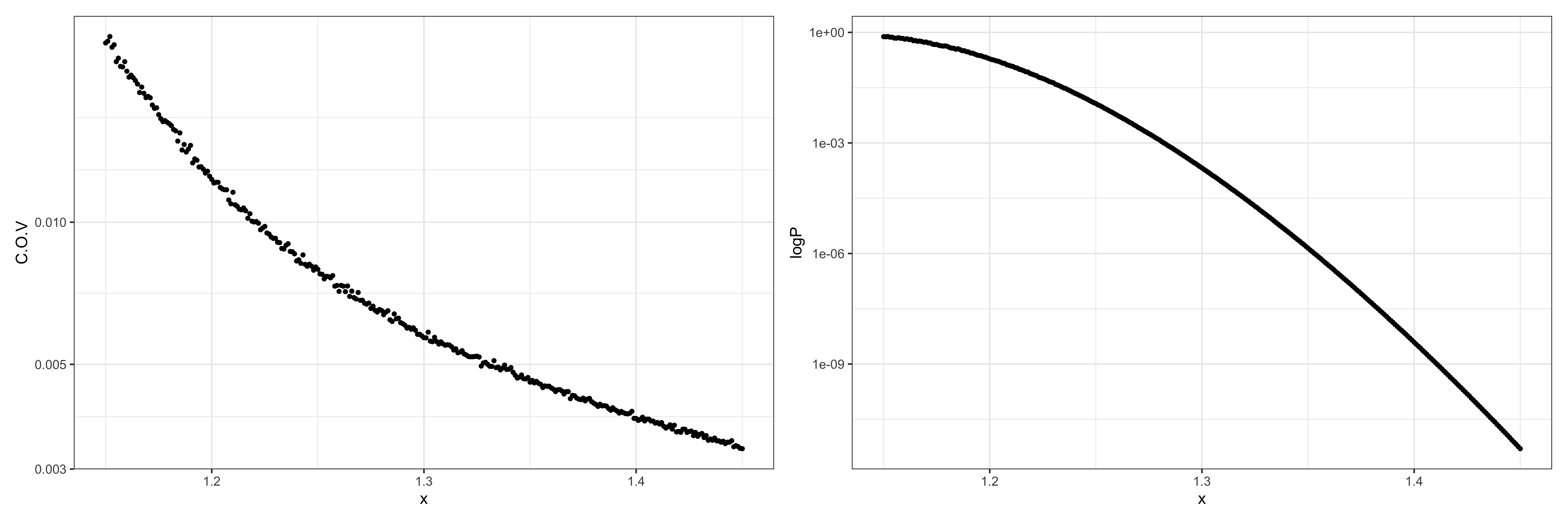
References

  • [1] Asmussen, S. and Kroese, D. (2006). Improved algorithms for rare event simulation with heavy tails. Adv. Appl. Probab., 38: 545-558.
  • [2] Asmussen, S. and Glynn, P. (2007). Stochastic Simulation: Algorithms and Analysis. Springer, New York.
  • [3] Bucklew, J. (2004). Introduction to Rare-Event Simulation. Springer, New York.
  • [4] Dembo, A. and Zeitouni, O. (1998). Large Deviations Techniques and Applications. Springer, New York.
  • [5] Dubbs, A. and Edelman, A. (2015). Infinite random matrix theory, tridiagonal bordered Toeplitz matrices, and the moment problem. Linear Algebra Appl., 467: 188-201.
  • [6] Dumitriu, I. and Edelman, A. (2002) Matrix models for beta ensembles. J. Math. Phys., 43(11): 5830-5847.
  • [7] Dumitriu, I. and Paquette, E. (2012). Global fluctuations for linear statistics of β𝛽\beta-Jacobi ensembles. Random Matrices Theo. 1, 1250013, 60pp.
  • [8] Gamboa, F., Rouault, A. (2011). Large deviations for random spectral measures and sum rules. Appl. Math. Res. Express AMRX. 2, 281-307.
  • [9] Huang, N. and Ma, Y-T.(2022) Limit theorems for beta-Laguerre and beta-Jacobi ensembles. Acta Math. Sci. 42B(5): 2025-2039.
  • [10] Jiang, T. (2013). Limit theorems for beta-Jacobi ensembles. Bernoulli, 19(3), 1028-1046.
  • [11] Jiang, T., Leder, K., and Xu, G. (2017). Rare-event analysis for extremal eigenvalues of white Wishart matrices. Ann. Stat., 45(4): 1609-1637.
  • [12] Johnstone, I. M. (2001). On the distribution of the largest eigenvalue in principal components analysis. Ann. Stat. 29: 295-327.
  • [13] Johnstone, I. M. . (2008). Multivariate analysis and Jacobi ensembles: largest eigenvalue, tracy–widom limits and rates of convergence. Ann. Stat., 36(6), 2638-2716.
  • [14] Juneja, S. and Shahabuddin, P. (2006). Rare event simulation techniques: An introduction and recent advances. In Handbook on Simulation (S. Henderson and B. Nelson, eds.) 291-350. North-Holland, Amsterdam.
  • [15] Killip, R. and Nenciu, I. (2004). Matrix models for circular ensembles, Int. Math. Res. Not. 50: 2665-2701.
  • [16] Ma, Y-T. (2023). Limits theorems and large deviations for β𝛽\beta-Jacobi ensembles at scaling temperatures. Acta Math. Sinica Ser. B. 39: 2054-2074.
  • [17] Lei, L. and Ma, Y-T.(2023) Large deviations for top eigenvalues of β𝛽\beta-Jacobi ensembles at scaling temperatures. Acta Math. Sci. 43: 1767-1780.
  • [18] Ma, Y-T. and Wang, S-Y. Rare-event analysis for extremal eigenvalues of β𝛽\beta-Jacobi matrices at any temperatures. Submitted.
  • [19] Muirhead, R. J. (1982). Aspects of Multivariate Statistical Theory. John Wiley & Sons, New York.
  • [20] Nagel, J. (2014) Nonstandard limit theorems and large deviations for the Jacobi beta ensembles. Random Matrices Theo., 3(3): 1450012.
  • [21] Pakzad, C. (2018). Large deviations principle for the largest eigenvalue of the Gaussian β𝛽\beta-Ensemble at high temperature. J. Theoret. Probab., 33: 428-443.
  • [22] Shwartz, A. and Weiss, A. (1995) Large Deviations for Performance Analysis. Chapman and Hall, London.