Multi-objective Evolution of Heuristic Using Large Language Model

Abstract

Heuristics are commonly used to tackle diverse search and optimization problems. Design heuristics usually require tedious manual crafting with domain knowledge. Recent works have incorporated large language models (LLMs) into automatic heuristic search leveraging their powerful language and coding capacity. However, existing research focuses on the optimal performance on the target problem as the sole objective, neglecting other criteria such as efficiency and scalability, which are vital in practice. To tackle this challenge, we propose to model heuristic search as a multi-objective optimization problem and consider introducing other practical criteria beyond optimal performance. Due to the complexity of the search space, conventional multi-objective optimization methods struggle to effectively handle multi-objective heuristic search. We propose the first LLM-based multi-objective heuristic search framework, Multi-objective Evolution of Heuristic (MEoH), which integrates LLMs in a zero-shot manner to generate a non-dominated set of heuristics to meet multiple design criteria. We design a new dominance-dissimilarity mechanism for effective population management and selection, which incorporates both code dissimilarity in the search space and dominance in the objective space. MEoH is demonstrated in two well-known combinatorial optimization problems: the online Bin Packing Problem (BPP) and the Traveling Salesman Problem (TSP). Results indicate that a variety of elite heuristics are automatically generated in a single run, offering more trade-off options than existing methods. It successfully achieves competitive or superior performance while improving efficiency up to 10 times. Moreover, we also observe that the multi-objective search introduces novel insights into heuristic design and leads to the discovery of diverse heuristics.

1 Introduction

Heuristics are commonly used in solving optimization and decision-making problems in a variety of fields, including engineering (Bozorg-Haddad, Solgi, and Loáiciga 2017), industry (Silver 2004), and economics (Vasant 2012). Unlike exact methods, heuristics offer practical alternatives for finding sub-optimal solutions within a reasonable time cost (Pearl 1984) and are particularly adept at handling complex problems with diverse attributes and constraints. However, developing effective heuristics usually demands expert knowledge and involves a laborious trial-and-error manual crafting, which poses a significant challenge for real-world applications.

To address this challenge, much effort has been devoted to automating the design of heuristics (Pillay and Qu 2021). These efforts can be broadly classified into three categories: heuristic configuration (Ramos et al. 2005; Visheratin, Melnik, and Nasonov 2016), heuristic selection (Tang et al. 2014; Xu, Hoos, and Leyton-Brown 2010), and heuristic composition (Burke et al. 2010; Drake et al. 2020; Pillay and Qu 2018). Despite the successful creation of novel heuristics, the effectiveness of these heuristics still heavily rely on algorithmic components crafted by human expert (Drake et al. 2020).

In recent years, large language models (LLMs) have demonstrated remarkable capabilities across various domains (Kaddour et al. 2023) including heuristic design. The integration of LLMs with evolutionary computation (EC) has enabled the automatic generation and refinement of heuristics along with their corresponding code implementations (Liu et al. 2024; Romera-Paredes et al. 2024; Ye et al. 2024). The designed heuristics achieved competitive performance with minimized human design and model training. However, all the existing LLM-based evolutionary heuristic search methods focus on a single objective regarding the optimized performance of the target problem (Ma et al. 2023; Nasir et al. 2024; Liu et al. 2024; Romera-Paredes et al. 2024; Zhang et al. 2024; Yao et al. 2024; van Stein and Bäck 2024; Li et al. 2024; Zeng et al. 2024; Mao et al. 2024; Ma et al. 2024). Other important heuristic design criteria, such as heuristic complexity (Ausiello et al. 2012) and code readability (Buse and Weimer 2009), which could be vital in practice, are neglected. While some studies have attempted to optimize multiple objectives by combining them into a single objective function, resulting in a single heuristic, the conflicting nature of diverse objectives often makes it challenging to find a single heuristic that satisfies all simultaneously. The exploration of effective methods for searching a set of non-dominated heuristics in a single run remains unexplored.

In this study, we model the automatic heuristic design as a multi-objective optimization problem (Dréo 2009) and propose the first LLM-based multi-objective heuristic search framework, termed Multi-objective Evolution of Heuristic (MEoH), to effectively search for a set of non-dominated heuristics in a single run. The contributions of this paper are as follows:

• We first propose an LLM-based automated heuristic design framework to consider the heuristic design from a multi-objective optimization perspective.

• We propose a dominance-dissimilarity mechanism to enhance diversity and improve search efficiency by considering both the dominance relationships in the objective space and the dissimilarity of heuristics in the search space.

• We demonstrate the superiority compared with the counterpart of single-objective LLM-based automated heuristic design on two classical optimization problems: the Traveling Salesman Problem (TSP) and the online Bin Packing Problem (BPP).

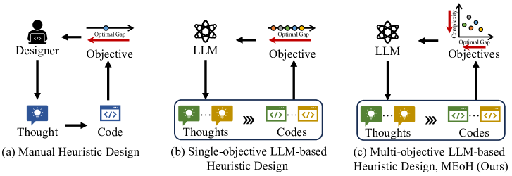
Figure 1: Comparison to human design and existing LLM-based heuristic design (a) manual heuristic design by human experts, (b) single-objective LLM-based heuristic design (e.g., FunSearch and EoH), and (c) our proposed multi-objective heuristic design (MEoH).

2 Related Works

2.1 Automated Heuristic Design

Automated heuristic design methods can be broadly classified into automated heuristic configuration, automated heuristic selection, and automated heuristic composition (Pillay and Qu 2021). The first category involves using optimization methods and machine learning techniques (Ramos et al. 2005; Visheratin, Melnik, and Nasonov 2016) to automatically adjust the parameters within a given algorithm framework (Agasiev and Karpenko 2017). The second category focuses on automatically choosing a suitable heuristic for each specific instance from a pool of existing heuristics (Tang et al. 2014; Xu, Hoos, and Leyton-Brown 2010). The third category combines various algorithmic elements to create novel heuristics  (Burke et al. 2010; Drake et al. 2020; Pillay and Qu 2018). While these methods have shown promise in enhancing the automation of heuristic design and improving performance, they still heavily rely on human-designed algorithmic components.

2.2 LLM-based Automated Heuristic Design

Large language models have shown remarkable performance across a variety of tasks and exhibit promising zero-shot capabilities in linguistic processing and code generation. The use of LLMs in automated heuristic design is still in its early stages. For example, FunSearch (Romera-Paredes et al. 2024) leverages LLMs to generate and improve code implementations of heuristics based on EC frameworks, achieving state-of-the-art results in mathematical and combinatorial optimization problems. EoH (Liu et al. 2024) evolves both idea descriptions and code implementations of heuristics simultaneously, leading to competitive performance in a more efficient manner. This EC+LLM approach has been successfully applied in heuristic and function design across various tasks such as reward function design (Ma et al. 2023), molecular design (Wang et al. 2024), network design (Mao et al. 2024), and Bayesian optimization (Yao et al. 2024). While effective heuristics are produced, they only consider the performance on target instances as the sole objective, without other critical objectives.

2.3 Multi-objective Heuristic Design

Dréo (2009) view automated heuristic design as a multi-objective problem, emphasizing the importance of identifying a set of non-dominated heuristics that can effectively balance optimality and efficiency. By automatically adjusting multiple sets of parameters for a heuristic (Dréo 2009; Dang and De Causmaecker 2014), it can be tailored to different scenarios. Zhang, Georgiopoulos, and Anagnostopoulos (2013) introduce S-Race, which employs a racing algorithm to automatically choose machine learning models based on multiple objectives. Furthermore, Blot et al. (2016) extend the single-objective heuristic configuration framework ParamILS to handle multiple objectives with MO-ParamILS. These methods rely on existing hand-crafted heuristics. Multi-objective genetic programming has also been applied on heuristic search (Schmidt and Lipson 2009; Vladislavleva, Smits, and Den Hertog 2008; Fan et al. 2024). However, they still demand existing hand-crafted primitives for defining and generating heuristics.

3 Preliminaries

3.1 Multi-objective Optimization

A multi-objective optimization problem (MOP) can be defined as

$$\min_{\boldsymbol{x}\in\mathcal{X}}\ \boldsymbol{f}(\boldsymbol{x})=(f_{1}(\boldsymbol{x}),f_{2}(\boldsymbol{x}),\ldots,f_{M}(\boldsymbol{x})),$$ (1)

where $\mathcal{X}$ represents the search space, $\boldsymbol{x}$ is a decision vector, and $\textbf{\em f}(\boldsymbol{x})$ is an $M$-objective vector to optimize. A non-trivial MOP cannot be solved by a single decision vector, and we have the following definitions for multi-objective optimization:

Pareto Dominance: Let $\boldsymbol{x}_{a},\boldsymbol{x}_{b}\in\mathcal{X}$, $\boldsymbol{x}_{a}$ is said to dominate $\boldsymbol{x}_{b}$ ($\boldsymbol{x}_{a}\prec\boldsymbol{x}_{b}$) if and only if $f_{i}(\boldsymbol{x}_{a})\leq f_{i}(\boldsymbol{x}_{b}),\forall i\in\{1,2,\ldots,M\}$ and $f_{j}(\boldsymbol{x}_{a})<f_{j}(\boldsymbol{x}_{b}),\exists j\in\{1,2,\ldots,M\}$.

Pareto Optimality: A decision vector $\boldsymbol{x}^{*}\in\mathcal{X}$ is Pareto-optimal if there does not exist $\boldsymbol{x}^{\prime}\in\mathcal{X}$ dominates $\boldsymbol{x}^{*}$, i.e., $\nexists\boldsymbol{x}^{\prime}\in\mathcal{X}$ such that $\boldsymbol{x}^{\prime}\prec\boldsymbol{x}^{*}$.

Pareto Set/Front: The set of all Pareto-optimal decision vectors is called the Pareto Set (PS), and its mapping in the objective space is called the Pareto Front (PF).

In this paper, we investigate multi-objective heuristic design. The decision vector $\boldsymbol{x}$ indicates the heuristic and the M-objective vector represents different criteria measuring different aspects of the performance of heuristics (e.g., optimal performance and complexity).

3.2 Multi-objective Evolutionary Algorithms

Multi-objective evolutionary algorithms (MOEAs) are among the most commonly used methods to solve MOPs. MOEAs work by maintaining a population of $N$ candidate individuals that evolve iteratively through genetic operators like crossover and mutation. There are three main paradigms for MOEAs: the dominance-based approach (Deb et al. 2002), the decomposition-based approach (Zhang and Li 2007), and the indicator-based approach (Zitzler and Künzli 2004).

4 Methodology

4.1 Framework

Multi-objective Evolution of Heuristic (MEoH) is a fusion of LLMs and multi-objective evolutionary optimization for effective multi-objective heuristic design. As is illustrated in Algorithm 1, MEoH commences with population initialization, where the population comprises heuristics, and progressively improves the population using MOEA until the termination condition is satisfied, to obtain a set of non-dominated heuristics that represent trade-offs among multiple objectives. Throughout each iteration, MEoH generates offspring using search operators. These operators are implemented through LLMs and predefined prompts to create offspring based on the selected parents from the population. New offspring are added to the population and population management is utilized to update the population to keep its size, with a focus on maintaining diversity and convergence. The dominance-dissimilarity mechanism is utilized in both parent selection and population management. Detailed explanations of each of these components will be provided in the subsequent sections.

MEoH represents a significant advancement in LLM-based heuristic design by extending the single-objective approach in existing works to the multi-objective scenarios and designing a set of non-dominated heuristics in a single run. Moreover, unlike directly combining MOEA and LLM-based heuristic search, MEoH introduces a unique dominance-dissimilarity measure to navigate the complex and discrete heuristic search space, overcoming challenges faced by conventional MOEAs like NSGA-II and MOEA/D.

1:  Input: Population size $N$; Maximum number of iterations $T$, Parent selection size $d$; Initial population $\boldsymbol{P}_{0}$; Pre-trained LLM $\mathcal{L}$.

2:  Output: Approximate Pareto-set $\boldsymbol{P}^{*}$.

3:  if $\boldsymbol{P}_{0}=\emptyset$ then

4:     for $i=1,\ldots,N$ do

5:        $o\leftarrow$ Generation($\mathcal{L}$);

6:        $\boldsymbol{P}_{0}\leftarrow\boldsymbol{P}_{0}\cup o$

7:     end for

8:  end if

9:  for $t=1,\ldots,T$ do

10:     for $i=1,\ldots,N$ do

11:        $\boldsymbol{P}_{parent}\leftarrow$ ParentSelection($\boldsymbol{P}_{t-1}$, $d$);

12:        $o\leftarrow$ Search($\mathcal{L},\boldsymbol{P}_{parent}$);

13:        $\boldsymbol{P}_{t-1}\leftarrow\boldsymbol{P}_{t-1}\cup o$

14:     end for

15:     $\boldsymbol{P}_{t}\leftarrow$ PopulationManagement($\boldsymbol{P}_{t-1},N$)

16:  end for

17:  $\boldsymbol{P}^{*}\leftarrow\boldsymbol{P}_{T}$

Algorithm 1 MEoH

4.2 Dominance-dissimilarity Mechanism

Traditional MOEAs (Deb et al. 2002; Zhang and Li 2007) and single-objective LLM-based heuristic design methods (Romera-Paredes et al. 2024; Liu et al. 2024) lack effective diversity maintenance strategies for multi-objective automated heuristic design. To address this, we propose a novel dominance-dissimilarity mechanism that considers both objective space dominance and heuristic search space dissimilarity.

Dominance Measure in Objective Space:

In the objective space, the Pareto dominance relationship between this pair of heuristics is evaluated, which is widely used in MOEAs (Zitzler and Thiele 1998; Deb et al. 2002).

Dissimilarity Measure in Search Space:

In the search space, the heuristics are represented through natural language descriptions and implemented in Python code. We evaluate the dissimilarity between code segments. Notably, there are various techniques available for this purpose, and we choose to utilize the widely adopted abstract syntax tree (AST) (Neamtiu, Foster, and Hicks 2005). The AST converts the code segment to an abstract syntactic structure (Baxter et al. 1998). And the similarity of code $a$ and code $b$ can be calculated based on the tree structures following Ren et al. (2020):

$$\text{Sim}_{\text{AST}}(a,b)=\text{Count}_{\text{clip}}(\text{Tree}_{a})/\text{Count}(\text{Tree}_{b}),$$ (2)

where $\text{Count}(\text{Tree}_{b})$ is the number of subtrees of $\text{Tree}_{b}$, and $\text{Count}_{\text{clip}}(\text{Tree}_{a})$ is the number of subtrees of $\text{Tree}_{a}$ that are matched the $\text{Tree}_{b}$. The AST similarity value ranges from 0 to 1, with 0 indicating complete dissimilarity between the two code segments and 1 signifying identical code segments. This approach allows for a quantitative assessment of the structural similarity between code segments, facilitating the comparison and evaluation of heuristics based on their code implementations.

Dominance-dissimilarity Score:

As illustrated in Figure 2, to determine the dominance-dissimilarity of each heuristic in the population, the dissimilarity, i.e., the negative AST similarity, between each pair of heuristics is calculated and stored in a matrix. Concurrently, in the objective space, the dominance relationship between each pair of heuristics is captured and represented as a mask with the same size as the dissimilarity matrix. Specifically, only the dominance relationship is accessible, while all other relationships are masked. Subsequently, the masked dissimilarity matrix is aggregated column-wise. The resulting dominance-dissimilarity score vector encapsulates both dominance and diversity aspects to guide the following parent selection and population management. The details can be found in Appendix A.

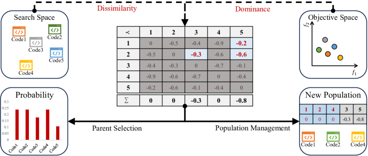
Figure 2: An illustration of parent selection and population management with dominance-dissimilarity mechanism. By incorporating code dissimilarity in the search space and dominance relationships in the objective space, the parent selection and population management are improved to foster diversity and search efficiency.

4.3 Heuristic Representation

Similar to Liu et al. (2024), each heuristic in MEoH is composed of three elements: a description in plain language, a code snippet in a specific format, and a fitness score.

The description is a brief linguistic explanation generated by LLMs that conveys the main idea. The code snippet is the actual implementation of the heuristic. In the experiments, we opted to use Python functions for implementation. The code snippet must include the 1) function name, 2) input variables, and 3) output variables for clarity. The fitness is evaluated on a set of instances for the specific target problem. Example heuristics can be found in Appendix G.

4.4 Heuristic Generation

Initial Heuristic Generation

The initial population of MEoH is comprised of heuristics. These heuristics can be generated by leveraging a LLM with a predefined generation prompt or by using human-designed existing heuristics. In order to fully demonstrate the capability of MEoH in designing competitive heuristics, we let LLM generate all the heuristics in both the initiation and evolution processes.

Offspring Heuristic Generation

The parent selection is the first step of generating offspring, in which a set of parent heuristics $\boldsymbol{S}$ are selected from the current population. In order to take into account the convergence and diversity of the heuristic search process, the dominance-dissimilarity score is employed to guide the probability of parent selection. A higher dominance-dissimilarity score indicates a lower likelihood of being dominated or a more diverse code segment, making it preferable. The parents are selected with probability proportional to their dominance-dissimilarity scores. The details can be found in Appendix A.

The parent heuristics are used as samples in the prompt to instruct LLM to generate offspring heuristics. We employ five different search operators with diverse prompt strategies adapted from EoH (Liu et al. 2024) to produce offspring heuristics. The details of these prompts can be found in Appendix F.

4.5 Population Management

As the offspring generated through search operations are incorporated into the population, the size of the population gradually increases. In order to ensure a consistent population size and update the population effectively, a population management strategy is proposed. The dominance-dissimilarity score is utilized for this purpose. Specifically, the heuristics in the population are sorted based on their dominance-dissimilarity score and the worst heuristics are removed to ensure that only the most promising individuals are retained within the population with details in Appendix A. By employing this strategy, the population is continually refined to maintain a high-quality and diverse set of individuals, enhancing the overall efficiency and effectiveness of the evolutionary process.

5 Experiments

5.1 Experimental Settings

Problems & Implementation Details

We demonstrate MEoH on two representative combinatorial optimization problems:

1) Online Bin Packing Problem: In online Bin Packing Problem (BPP) (Seiden 2002), a set of items, each with its own weight, needs to be packed into bins with a predetermined capacity. The objective of the BPP is to minimize the total number of bins required to accommodate all the items. In an online scenario, items are packed as they are received without prior knowledge. The generated heuristics are evaluated on $5$ Weibull instances with $5,000$ items (referred to as 5k), and the capacity of bins is $100$.

We inherit the settings from Romera-Paredes et al. (2024) to design constructive heuristics for aligning the arriving items to the appropriate bins. The designed heuristics involve a function scoring the bins, where the input includes the arriving item size and the remaining capacities of the bins. The item with the highest score will be assigned to the bin.

2) Travelling Salesman Problem: In Traveling Salesman Problem (TSP) (Reinelt 2003), the objective is to find the shortest route that visits all given nodes exactly once and returns to the starting node. In this work, we evaluate the fitness of designed heuristics during evolution on $64$ instances with $100$ nodes. The coordinate of each node is randomly sampled from $[0,1]$ (Kool, van Hoof, and Welling 2018).

The Guided Local Search (GLS) framework is employed (Voudouris, Tsang, and Alsheddy 2010) to iteratively improve the solution quality following (Liu et al. 2024). GLS iteratively performs two steps: 1) local search and 2) perturbation. Until the stop criterion is satisfied, the best solution obtained throughout the iterations is considered the final solution. We aim to design a heuristic to update the distance matrix in the perturbation step.

The experimental parameter settings are as follows: the number of generations is $20$, and the population size is $20$ and $10$ for online BPP and TSP, respectively. Each crossover operator selects 5 parent heuristics to reproduce the offspring heuristics. The number of iterations and running time in the GLS for TSP is limited to $1,000$ and $60$ seconds.

Environments

To ensure fairness and consistency, all experiments in this study were conducted on a computer equipped with an Intel Core i7-11700 processor and 32GB of memory. GPT3.5-turbo is employed as the per-trained LLM.

Performance Metric

Objectives

1) Optimal Gap: We use the heuristic’ optimal gap to baseline as the first objective (e.g., the gap of the number of bins used in designed heuristics to the lower bound of bin number). 2) Efficiency: The running time of heuristics is used as the second objective to represent the efficiency of heuristics.

Metric

1) Hypervolume: The Hypervolume(HV) is a commonly used metric in multi-objective optimization. It provides a comprehensive assessment of convergence and diversity of the approximate Pareto front without the ground truth Pareto front (Audet et al. 2021). A larger HV value indicates a better performance. 2) IGD: The Inverted Generational Distance(IGD) measures the quality of the generated approximate Pareto front in relation to the reference set. Here the reference set is the nondominated set derived from the union of all generated heuristics. A lower IGD value is preferred, which indicates better convergence and diversity, implying that the generated solutions are closer to the reference set. The detailed formulation of two metrics can be found in Appendix D.

Baseline Methods

In this study, our primary focus lies in exploring LLM-based automated heuristic design approaches. Consequently, we compare the two closest related works, namely FunSearch (Romera-Paredes et al. 2024) and EoH (Liu et al. 2024). The details can be found in Appendix C.

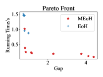
(a) Pareto Front

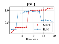
(b) HV

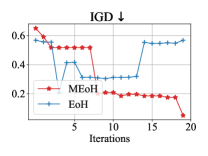
(c) IGD

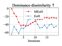
(d) Score

Figure 3: Comparations of EoH and MEoH on BPP5k.

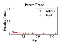
(a) Pareto Front

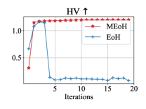
(b) HV

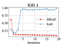
(c) IGD

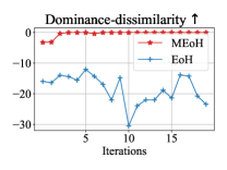
(d) Score

Figure 4: Comparations of EoH and MEoH on TSP100.

5.2 Experimental Results

Convergence Analysis

1) BPP: The curve of HV and IGD for the heuristic populations generated in each iteration are displayed in Figure 3(b) and (c), respectively. As EoH only pursues optimal gap without considering diversity, the HV and IGD become worse as the evolution progresses. In contrast, MEoH systematically takes into account both the optimal gap and running time. As a result, MEoH achieves notably higher HV and lower IGD, indicating significantly better multi-objective trade-off results. Figure 4(b) and (c) provide more evidence. MEoH converges faster and clearly outperforms EoH in terms of HV and IGD.

Pareto Fronts

Figure 3(a) and Figure 4(a) compare the approximate non-dominated heuristics of the final population obtained by MEoH and EoH. Results show that 1) MEoH generates a diverse set of heuristics with different trade-offs over the two objective. In contrast, EoH only finds similar heuristics that cover a much smaller region in the objective space. 2) The heuristics obtained from MEoH can significantly reduce the running time (up to 10 times) when achieving a similar optimal gap.

Performance Measurement

1) BPP: To comprehensively evaluate the performance of our MEoH in more general cases, we test FunSearch, EoH, and MEoH on various problem instances with different sizes and capacities. The problem sizes in our test include 5k, 10k, and 100k, and the capacities of the bins are set at $100$ and $500$. Each test set consists of five instances sampled from Weibull distribution (Romera-Paredes et al. 2024). The average gap with reference to the relaxation lower bound $lb$ and the running time are shown in Table 1. For the in-distribution instances, i.e., the bin capacity is $100$, all of these three frameworks exhibit promising performance in terms of the optimal gap, and the running time of MEoH heuristics are significantly less than the counterparts of FunSearch and EoH, especially in large-size instances, i.e., BPP100k. MEoH heuristics achieve competitive performance compared to EoH but do so in significantly less running time (up to 10 times faster). In contrast, for out-distribution instances, i.e., the bin capacity is $500$, the performance of FunSearch heuristics drastically deteriorates in terms of the optimal gap. On the other hand, both EoH and MEoH heuristics exhibit promising performances in such scenarios. Notably, MEoH demonstrates a balanced trade-off between the optimal gap and running time, showcasing its effectiveness in handling out-distribution instances efficiently.

Table 1: Results of In- and Out-of-distribution BPP.

Weibull	FunSearch		EoH		MEoH
	Gap	Time/s	Gap	Time/s	Gap	Time/s
5k C100	0.802%	0.728	lightgray 0.753%	1.362	1.387%	lightgray 0.191
10k C100	2.595%	2.128	lightgray 0.537%	5.128	0.651%	lightgray 0.650
100k C100	3.319%	195.734	0.391%	502.938	lightgray 0.080%	lightgray 59.078
Avg.	2.239%	66.197	lightgray0.560%	169.809	0.706%	lightgray19.973
5k C500	29.494%	0.750	lightgray0.100%	1.672	0.351%	lightgray0.100
10k C500	47.734%	2.459	lightgray0.125%	6.337	0.473%	lightgray0.306
100k C500	53.640%	259.094	lightgray0.099%	646.828	0.410%	lightgray22.078
Avg.	43.623%	87.434	lightgray 0.108%	218.279	0.411%	lightgray 7.495

1) TSP: We evaluate these three methods on randomly generated TSP instances comprising $100$, $500$, and $1,000$ nodes and a variety of TSP instances with up to $1,002$ nodes from TSPLIB (Reinelt 1991). Table 2 and Table 3 display the gap compared to the best-known solution (for the randomly generated instances, the best-known solutions are obtained using the Concorde solver (Applegate et al. 2006)) and the corresponding running times. As shown in Table 2, FunSearch and MEoH (Best) heuristics exhibit promising performance on TSP100 and TSP500 instances. In general, MEoH provides a set of heuristics that enable trade-offs between optimality and efficiency. As shown in Table 3, for smaller instances (up to $200$ nodes), the MEoH heuristics demonstrate superior performance in terms of both the optimal gap and running time. For larger instances ($200$ to $1,002$ nodes), MEoH still outperforms in running time, although slightly lagging behind EoH in terms of the optimal gap.

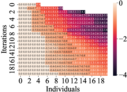
(a) BPP, MEoH

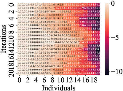
(b) BPP, EoH

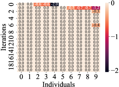
(c) TSP, MEoH

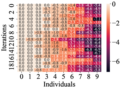
(d) TSP, EoH

Figure 5: Visualization of the evolution of dominance-dissimilarity score.

Table 2: Results of in- and out-of-distribution randomly generated TSP.

	TSP100		TSP500		TSP1000
	Gap	Time/s	Gap	Time/s	Gap	Time/s
FunSearch	lightgray0.100%	1.452	lightgray1.525%	27.598	lightgray2.344%	161.124
EoH	0.113%	22.434	1.750%	43.541	2.524%	262.603
MEoH(Best)	0.109%	1.373	1.733%	30.945	4.208%	26.844
MEoH(Fast)	3.690%	lightgray0.175	4.402%	lightgray3.306	4.536%	lightgray21.900

Table 3: Results of small and large TSPLIB instances.

TSPLIB	FunSearch		EoH		MEoH
	Gap	Time/s	Gap	Time/s	Gap	Time/s
berlin52	0.000%	0.484	0.000%	8.500	0.000%	lightgray0.344
ch130	lightgray 0.156%	2.031	0.233%	42.360	0.233%	lightgraylightgray1.016
ch150	0.306%	2.500	0.502%	56.062	lightgray0.000%	lightgray1.250
eil101	lightgray0.000%	28.391	0.373%	56.031	lightgray0.000%	2lightgray2.297
eil51	0.000%	0.515	0.000%	7.109	0.000%	lightgray0.312
eil76	0.183%	0.938	0.107%	14.844	lightgray0.000%	lightgray0.531
kroA100	0.000%	1.407	0.000%	24.437	0.000%	lightgray0.734
kroC100	0.000%	1.500	0.000%	24.781	0.000%	lightgray0.703
kroD100	0.000%	1.578	0.000%	24.563	0.000%	lightgray0.734
lin105	0.000%	1.812	0.000%	26.703	0.000%	lightgray0.890
pr76	0.000%	0.969	0.000%	14.469	0.000%	lightgray0.546
rd100	0.000%	1.453	0.000%	24.266	0.000%	lightgray0.750
st70	0.000%	0.859	0.000%	12.797	0.000%	lightgray0.500
Avg.	0.050%	3.418	0.093%	25.917	lightgray0.018%	lightgray2.354
a280	0.195%	378.656	lightgray0.059%	640.453	1.245%	lightgray356.468
pcb442	1.389%	932.093	1.714%	1694.547	lightgray1.284%	lightgray916.219
pr1002	2.878%	354.813	lightgray2.487%	3592.891	3.272%	lightgray142.000
tsp225	1.679%	12.891	1.243%	136.078	lightgray0.197%	lightgray8.328
Avg.	1.535%	419.613	lightgray1.376%	1515.992	1.50%	lightgray355.754

Table 4: Two top heuristics designed by MEoH.

	TSPLIB		BPP C100
	Gap	Time/s	Gap	Time/s
FunSearch	0.050%	3.418	2.239%	66.197
EoH	0.093%	25.917	lightgray0.560%	169.809
MEoH (Best)	lightgray0.018%	2.354	0.706%	19.973
MEoH (Fast)	3.563%	lightgray0.138	4.326%	lightgray6.533

5.3 Comparison to Conventional MOEAs

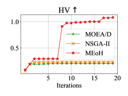
(a) HV

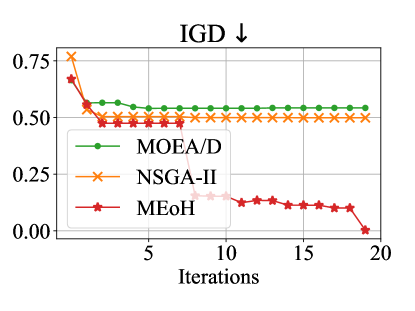
(b) IGD

Figure 6: Comparison to conventional MOEAs.

In this section, we evaluate the impact of our proposed dominance-dissimilarity mechanism on the optimization process and compare to two representative MOEAs: NSGA-II (Deb et al. 2002) and MOEA/D (Zhang and Li 2007).

Figure 6 depicts the results on BPP. MEoH can obtain the best HV and IGD. Our findings highlight the effectiveness of our dominance-dissimilarity mechanism, which integrates considerations from both the search and objective spaces, in improving the optimization process.

5.4 Visualization of Dominance-dissimilarity Scores

We visualize the evolution of Dominance-dissimilarity Scores in Figure 5. The x-axis is the heuristic index, and the y-axis is the iteration index. It is important to note that the presence of blank blocks in the early iterations indicates cases where the population is not filled, due to the generation of illegal code segments by LLM. As shown in Figure 5, MEoH heuristics can maintain diversity during the evolutionary process, while the diversity of EoH drastically deteriorates. We also depict the average dominance-dissimilarity score, as depicted in Figure 3 (d) and Figure 4 (d). Results demonstrate the superiority of MEoH and the efficiency of our dominance-dissimilarity mechanism in maintaining population diversity.

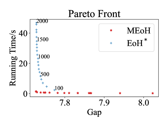
Figure 7: Comparations of the non-dominated heuristics of MEoH and the any-time performance the best heuristic generated by EoH (termed as $EoH^{*}$) on TSP.

5.5 Comparison to Any-time Performance

The performance of a single heuristic at any given time can provide a set of heuristics that offer different trade-offs between optimal gap and running time. For instance, reducing the number of iterations in GLS from $1,000$ to $100$ results in a decrease in running time but a deterioration in the optimal gap. By comparing the heuristics generated by MEoH to the best heuristic produced by EoH, we can further illustrate the benefits of multi-objective heuristic design. We evaluate the performance of the best EoH heuristic with varying numbers of iterations. Figure 7 demonstrates that the heuristics generated by MEoH outperform those of EoH. Even the best EoH heuristic with 100 iterations falls short in terms of running time and optimal gap compared to all MEoH heuristics. Additionally, while the best EoH heuristic with $2,000$ iterations can achieve competitive optimality, it lags behind in running time by approximately 20 times.

6 Conclusion, Limitation, and Future Work

Conclusion

This paper developes a novel framework, termed MEoH, for LLM-based multi-objective automatic heuristic design. We propose a dominance-dissimilarity mechanism for effective search in the discrete and complex heuristic space. We demonstrate MEoH on two widely-studied combinatorial optimization problems to optimize both heuristics’ optimal gap and running time. Results show that MEoH significantly outperforms existing LLM-based heuristic design methods including FunSearch and EoH in producing trade-off heuristics over multiple objectives. The efficiency can be increased dramatically up to 10 times with a close optimal gap. Moreover, additional ablation studies and visualization of the evolution process validate the superiority of MEoH over conventional MOEAs and the effectiveness of the proposed dominance-dissimilarity mechanism in multi-objective automatic heuristic design.

Limitation and Future Work

While we have demonstrated the effectiveness of MEoH, we only test it on two objectives. We want to investigate the performance of MEoH on many-objective cases and more heuristic design tasks.

Appendix A Algorithm Details

In this part, we elaborate on the details of parent selection and population management used in our proposed MEoH, as shown in Algorithm 1 and Algorithm 2, respectively.

Calculation of Dominance-dissimilarity Score

The lines 3-16 in Algorithm 1 and the lines 4-17 in Algorithm 2 are almost identical, illustrating the computation of the dominance-dissimilarity score. Specifically, two square matrices, namely the dissimilarity score matrix $\boldsymbol{S}$ and the dominance mask matrix $\boldsymbol{D}$, are initialized to be zeros. Each heuristic within the population is compared in pairs, with their dissimilarity (negative AST similarity) and dominance relationships recorded in the corresponding matrices. Subsequently, these matrices are element-wise multiplied to yield the dominance-dissimilarity score matrix $\boldsymbol{S}^{\prime}$. The dominance-dissimilarity vector $\boldsymbol{v}$ is then derived by summing the columns of $\boldsymbol{S}^{\prime}$. This vector encapsulates a blend of dominance and dissimilarity considerations, guiding the following parent selection and population management.

Parent Selection

For parent selection, as delineated in Algorithm 1, the dominance-dissimilarity vector $\boldsymbol{v}$ is leveraged to construct a probability distribution $\boldsymbol{\pi}$ using the softmax function. The parents are subsequently sampled based on this distribution to strike a balance between exploration and exploitation.

Population Management

For population management, as shown in Algorithm 2, the dominance-dissimilarity vector $\boldsymbol{v}$ is descending sorted, and the resulting indices $\boldsymbol{k}$ are utilized to truncate the population, and the first $N$ individuals consists the new population $\boldsymbol{P}^{\prime}$.

1:  Input: Population $\boldsymbol{P}$; Population size $N$; Parent selection size $d$.

2:  Output: Selected parents $\boldsymbol{P}_{parent}$.

3:  Initialize the dissimilarity score matrix $\boldsymbol{S}$ as an $N\times N$ matrix filled with zeros;

4:  Initialize the dominance mask matrix $\boldsymbol{D}$ as an $N\times N$ matrix filled with zeros;

5:  for $i=1,\ldots,N$ do

6:     for $j=1,\ldots,N$ do

7:        if $i\neq j$ then

8:           $\boldsymbol{S}[i,j]\leftarrow-$AST($\boldsymbol{P}[i],\boldsymbol{P}[j]$);

9:           if $\boldsymbol{P}[i]\prec\boldsymbol{P}[j]$ then

10:              $\boldsymbol{D}[i,j]\leftarrow 1$;

11:           end if

12:        end if

13:     end for

14:  end for

15:  $\boldsymbol{S}^{\prime}\leftarrow\boldsymbol{S}\odot\boldsymbol{D}$

16:  $\boldsymbol{v}\leftarrow$ ColumnwiseSum($\boldsymbol{S}^{\prime}$)

17:  $\boldsymbol{\pi}\leftarrow$ Softmax($\boldsymbol{v}$)

18:  $\boldsymbol{P}_{parent}\leftarrow$ Sample($\boldsymbol{P},\boldsymbol{\pi},d$)

Algorithm 1 ParentSelection

1:  Input: Population $\boldsymbol{P}$; Population size $N$.

2:  Output: New population $\boldsymbol{P}^{\prime}$.

3:  Current population size $N^{\prime}\leftarrow$ size($\boldsymbol{P}$)

4:  Initialize the dissimilarity score matrix $\boldsymbol{S}$ as an $N^{\prime}\times N^{\prime}$ matrix filled with zeros;

5:  Initialize the dominance mask matrix $\boldsymbol{D}$ as an $N^{\prime}\times N^{\prime}$ matrix filled with zeros;

6:  for $i=1,\ldots,N$ do

7:     for $j=1,\ldots,N$ do

8:        if $i\neq j$ then

9:           $\boldsymbol{S}[i,j]\leftarrow-$AST($\boldsymbol{P}[i],\boldsymbol{P}[j]$);

10:           if $\boldsymbol{P}[i]\prec\boldsymbol{P}[j]$ then

11:              $\boldsymbol{D}[i,j]\leftarrow 1$;

12:           end if

13:        end if

14:     end for

15:  end for

16:  $\boldsymbol{S}^{\prime}\leftarrow\boldsymbol{S}\odot\boldsymbol{D}$

17:  $\boldsymbol{v}\leftarrow$ ColumnwiseSum($\boldsymbol{S}^{\prime}$)

18:  $\boldsymbol{k}\leftarrow$ DescendingSortedIndexes($\boldsymbol{v}$)

19:  Initialize a new population $\boldsymbol{P}^{\prime}\leftarrow\emptyset$

20:  for $i=1,\ldots,N$ do

21:     $\boldsymbol{P}^{\prime}\leftarrow\boldsymbol{P}^{\prime}\cup\boldsymbol{P}[\boldsymbol{k}[i]]$

22:  end for

Algorithm 2 PopulationManagement

Appendix B Heuristic Design Task Details

We demonstrate the proposed method on two heuristic design tasks: 1) heuristics design for online Bin Packing Problem (BPP) and 2) heuristic design for guided local search for Traveling Salesman Problem (TSP). We introduce the detailed heuristic design settings for each task.

B.1 BPP

In online Bin Packing Problem (BPP) (Seiden 2002), a set of items, each with its own weight, needs to be packed into bins with a predetermined capacity. The objective of the BPP is to minimize the total number of bins required to accommodate all the items. In an online scenario, items are packed as they are received without prior knowledge.

The heuristic operates by loading items sequentially in an online fashion, requiring only the selection of the best bin at each iteration. This designed function scores bins based on their remaining capacities and the size of the arriving item, with the highest scoring bin chosen for each iteration. The function takes two inputs - the size of the arriving item and the remaining capacities of the bins - and outputs a vector that ranks the bins accordingly. A task description used in the prompt and the Python code snippet requirements are illustrated as follows:

Task Description: I need help designing a novel score function that scoring a set of bins to assign an item. In each step, the item will be assigned to the bin with the maximum score. If the rest capacity of a bin equals the maximum capacity, it will not be used. The final goal is to minimize the number of used bins. Code Requirements: Implement it in Python as a function named “score”. This function should accept 2 inputs: [“item”, “bins”]. The function should return 1 output: [“scores”]. “item” and “bins” are the size of current item and the rest capacities of feasible bins, which are larger than the item size. The output named “scores” is the scores for the bins for assignment. Note that “item” is of type int, “bins” is a Numpy array include integer values, and “scores” should be Numpy array. Avoid utilizing the random component, and it is crucial to maintain self-consistency.

Figure 1: BPP heuristic design description and code requirement.

B.2 TSP

For TSP, one of the widely used metaheuristics, Guided Local Search (GLS), is used (Voudouris, Tsang, and Alsheddy 2010). The pipeline of GLS is as follows:

Step 1: Create an initial solution using nearest neighbor constructive heuristics.

Step 2: Local Search Stage: Perform a local search (swap and relocate) to improve the current solution and generate a local optimal solution.

Step 3: Perturbation Stage: Update the distance matrix. Perform another local search based on the updated distance matrix to perturb the local optimal solution to escape from local optimality.

Steps 2 and 3 are iteratively repeated until the stopping criterion (maximum number of iterations set to $1,000$ in the experiments) is satisfied. The best solution obtained throughout the iterations is considered the final solution.

Our goal is to develop a heuristic to update the distance matrix in the perturbation step. The task description provided in the prompt and the requirements for the Python code snippet are outlined below. The inputs include the original distance matrix, the local optimal solution, and the frequency of edge usage in perturbation. The output should be the updated distance matrix.

Task Description: Given an edge distance matrix and a local optimal route, please help me design a strategy to update the distance matrix to avoid being trapped in the local optimum with the final goal of finding a tour with minimized distance. You should create a heuristic for me to update the edge distance matrix. Code Requirements: Implement it in Python as a function named “update_edge_distance”. This function should accept 3 inputs: [“edge_distance”, “local_opt_tour”, “edge_n_used”]. The function should return 1 output: “updated_edge_distance”]. “local_opt_tour” includes the local optimal tour of IDs, “edge_distance” and “edge_n_used” are matrixes, “edge_n_used” includes the number of each edge used during permutation. All are Numpy arrays.

Figure 2: TSP heuristic design task description and code requirement.

Appendix C Baseline Settings

In this work, we employ FunSearch (Romera-Paredes et al. 2024) and EoH (Liu et al. 2024) as baseline. For EoH, we inherit the default settings, including the number of iterations $T=20$, the parent selection size $d=5$, and the population size $N=10$ for the TSP and $N=20$ for the BPP. Our MEoH also follows these settings. In summary, $1,000$ heuristics are generated for solving TSP, and $2,000$ heuristics for BPP. For FunSearch, we also adopt the default settings, the number of islands is $10$ and the number of samples for each prompt is $4$. FunSearch generates $10,000$ heuristics for solving BPP and TSP.

Appendix D Metric Definition

D.1 HV

Hypervolume (HV) is calculated as follows:

$${\rm HV}(\mathcal{P},\boldsymbol{r}^{*})={\rm VOL}\Big{(}\mathop{\cup}\limits_{\boldsymbol{v}\in\mathcal{P}}[v_{1},r_{1}^{*}]\times\ldots\times[v_{m},r_{m}^{*}]\Big{)},$$ (3)

where $\mathcal{P}$ represents the approximate Pareto front obtained by an automated algorithm design approach, $\boldsymbol{v}=(v_{1},\ldots,v_{m})^{\intercal}$ denotes the corresponding objective vector, ${\rm VOL}(\cdot)$ represents the Lebesgue measure, and $\boldsymbol{r}^{*}=(r_{1}^{*},\ldots,r_{m}^{*})^{\intercal}$ is a reference objective vector.

To account for variations in HV values across different objective domains, i.e., the scalar of intrinsic objective value and the running time, we normalized each objective value for each instance. Specifically, the generated algorithm $\boldsymbol{x}$ can be normalized in the objective space using the approximated ideal point $\boldsymbol{z}^{\text{ideal}}=(z_{1}^{\text{ideal}},\ldots,z_{M}^{\text{ideal}})^{\intercal}$ and the approximated nadir point $\boldsymbol{z}^{\text{nadir}}=(z_{1}^{\text{nadir}},\ldots,z_{M}^{\text{nadir}})^{\intercal}$ derived from the union of all approximated Pareto-front $\mathcal{P}$ as

$$f_{i}^{\prime}(\boldsymbol{x})=\frac{f_{i}(\boldsymbol{x})-z_{i}^{\text{ideal}}}{z_{i}^{\text{nadir}}-z_{i}^{\text{ideal}}},$$ (4)

where $z_{i}^{\text{ideal}}=\min\{v_{i}|\boldsymbol{v}\in\mathcal{P}\}$ and $z_{i}^{\text{nadir}}=\max\{v_{i}|\boldsymbol{v}\in\mathcal{P}\}$, $\forall i\in\{1,\ldots,M\}$. Consequently, the value of each objective is normalized to $[0,1]$. Based on that, the reference point $\boldsymbol{r}^{*}=(1.1,\ldots,1.1)^{\intercal}$.

D.2 IGD

Inverted Generational Distance (IGD) measures the convergence and diversity of the obtained Pareto front approximation concerning the true Pareto front. It is calculated as follows:

$$\text{IGD}(P,P^{*})=\frac{1}{{\lvert P^{*}\rvert}}\sum_{p\in P^{*}}\min_{q\in P}d(p,q),$$ (5)

where $P$ is the set of decision vectors, i.e, the approximated Pareto front. $P^{*}$ is the true Pareto front, $\lvert P^{*}\rvert$ is the number of points in the true Pareto front $d(p,q)$ is the Euclidean distance between the points $p$ and $q$ in the objective space.

The IGD calculates the average distance from the true Pareto front points to their nearest neighbor in the approximated Pareto front. A lower IGD value indicates a better approximation of the true Pareto front.

It’s important to note that the true Pareto front is required for calculating the IGD metric, which may not always be available in many cases. So, a reference set of well-distributed Pareto-optimal solutions is often used as an approximation of the true Pareto front, here the reference set is the nondominated set derived from the union of all generated heuristics.

Appendix E Additional Experimental Results

In this section, we assess the influence of our proposed dominance-dissimilarity mechanism on the optimization process and compare to two representative MOEAs: NSGA-II (Deb et al. 2002) and MOEA/D (Zhang and Li 2007). The experiments are conducted consistently across identical experimental settings, with each experiment repeated three times to ensure the robustness and reliability of the results. To enhance clarity, the standard deviation, represented by the shaded area, is reduced by a factor of $0.3$.

As shown in Figure 3 and Figure 4, compared NSGA-II and MOEA/D, our MEoH can achieve the best HV and IGD on both BPP and TSP. These findings demonstrate the effectiveness of our dominance-dissimilarity mechanism, which integrates considerations from both the search and objective spaces, in improving the optimization process.

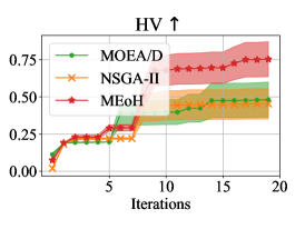
(a) HV

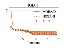
(b) IGD

Figure 3: Comparison to conventional MOEAs on BPP.

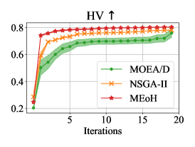
(a) HV

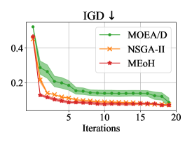
(b) IGD

Figure 4: Comparison to conventional MOEAs on TSP.

Appendix F Search Operators

MEoH inherits $5$ search operators from EoH (Liu et al. 2024). These operators are all implemented based on LLMs. In this part, the corresponding prompts will be elaborated. Generally, the prompt consists of operator-specific guidance, task description, and code requirements. For brevity, the task description and the code requirements are denoted as $Task Description and $Code Requirements, respectively.

F.1 E1 Operator

As shown in Figure 5, the E1 operator is used to explore a new heuristic different from the $5$ selected heuristics. For simplicity, the heuristics including corresponding algorithm description and code are omitted.

$Task Description I have $5$ existing algorithms with their codes as follows: $<$Algorithm description$>$: … $<$Code$>$: … … Please help me create a new algorithm that has a totally different form from the given ones. First, describe your new algorithm and main steps in one sentence. The description must start with “$<$start$>$” and end with “$<$end$>$”. Next, $Code Requirements Your Python code should be formatted as a Python code string: “python … ” Be creative and do not give additional explanation.

Figure 5: An example of E1 prompt for TSP

F.2 E2 Operator

As shown in Figure 6, the E2 operator is used to generate a new heuristic based on the common idea of the $5$ selected heuristics.

$Task Description I have $5$ existing algorithms with their codes as follows: $<$Algorithm description$>$: … $<$Code$>$: … … Please help me create a new algorithm that has a totally different form from the given ones. First, describe your new algorithm and main steps in one sentence. The description must start with “$<$start$>$” and end with “$<$end$>$”. Next, $Code Requirements Your Python code should be formatted as a Python code string: “python … ” Be creative and do not give additional explanation.

Figure 6: An example of E2 prompt for TSP

F.3 M1 Operator

As shown in Figure 7, the M1 operator is desired to generate a new heuristic based on a given heuristics to improve the performance.

$Task Description I have one algorithm with its code as follows: $<$Algorithm description$>$: … $<$Code$>$: … … Please assist me in creating a new algorithm that has a different form but can be a modified version of the algorithm provided. First, describe your new algorithm and main steps in one sentence. The description must start with “$<$start$>$” and end with “$<$end$>$”. Next, $Code Requirements Your Python code should be formatted as a Python code string: “python … ” Be creative and do not give additional explanation.

Figure 7: An example of M1 prompt for TSP

F.4 M2 Operator

As shown in Figure 8, the goal of the M2 operator is to modify the parameters of a given heuristic.

$Task Description I have one algorithm with its code as follows: $<$Algorithm description$>$: … $<$Code$>$: … Please identify the main algorithm parameters and assist me in creating a new algorithm that has a different parameter settings of the score function provided. First, describe your new algorithm and main steps in one sentence. The description must start with “$<$start$>$” and end with “$<$end$>$”. Next, $Code Requirements Your Python code should be formatted as a Python code string: “python … ” Be creative and do not give additional explanation.

Figure 8: An example of M2 prompt for TSP

F.5 M3 Operator

In Figure 9, the M3 operator is used to simplify a given heuristic by eliminating redundant components. In this context, the task description is not required. Furthermore, only the part introducing the input and output from code requirements is needed.

First, you need to identify the main components in the function below. Next, analyze whether any of these components can be overfit to the in-distribution instances. Then, based on your analysis, simplify the components to enhance the generalization to potential out-of-distribution instances. Finally, provide the revised code, keeping the function, inputs, and outputs unchanged. $<$Code$>$: … “local_opt_tour” includes the local optimal tour of IDs, “edge_distance” and “edge_n_used” are matrixes, “edge_n_used” includes the number of each edge used during permutation. All are Numpy arrays. Your Python code should be formatted as a Python code string: “python … ” Be creative and do not give additional explanation.

Figure 9: An example of M3 prompt for TSP

Appendix G Designed Heuristics

In this section, we present a variety of representative heuristics designed by LLM-based automated heuristic design frameworks, encompassing FunSearch (Romera-Paredes et al. 2024), EoH (Liu et al. 2024), and our own MEoH.

G.1 BPP

EoH Heuristics

The heuristic developed by EoH with the best performance in terms of the optimal gap, as shown in Figure 10, utilizes sophisticated mathematical operators such as logarithm, square root, and exponential. The complexity of this scoring function renders it challenging to construct manually due to its intricate nature and reliance on advanced mathematical operations.

Algorithm Description: My new algorithm calculates the score for each bin as the sum of the bin’s current capacity divided by the product of the logarithm of the difference between the bin’s capacity and the item size and the square root of the difference between the bin’s capacity and the item size, raised to the power of the bin’s current capacity, and multiplied by the exponential function raised to the power of the item size multiplied by the difference between the bin’s capacity and the item size. Additionally, the score is multiplied by the reciprocal of the bin’s current capacity to prioritize bins with lower capacities. ⬇ 1 2import numpy as np 3\pardef score(item, bins): 4scores = (bins / ((np.log(bins - item) * np.sqrt(bins - item)) ** bins)) * np.exp(item * (bins - item)) * (1/bins) 5return scores

Figure 10: The EoH heuristic with the best optimal gap on BPP.

FunSearch Heuristics

The heuristic devised by FunSearch, illustrated in Figure 11, it incorporates numerous sophisticated parameters and introduces a random noise. Unlike the EoH approach, the FunSearch heuristic relies on intricate parameter settings and stochastic perturbations for optimization.

⬇ 1 2def priority(item: float, bins: np.ndarray) -> np.ndarray: 3eps = 1e-7 4\par# Calculate scores based on available space and current capacity 5scores = (bins - item) / (bins + eps) 6\par# Adjust the penalty if necessary 7penalty = np.power(np.min(bins), 0.5) * np.arange(len(bins)) * 0.01 8scores -= penalty 9\par# Scale the scores and add a weight 10weight = 0.8 11scores = (scores - np.min(scores)) / (np.max(scores) - np.min(scores)) * (1 - weight) + weight 12\par# Favor bins where the item fits perfectly 13scores += 0.5 * (bins == item) 14\par# Favor bins with relatively higher remaining capacity 15scores += 0.02 * (bins - item) / np.max(bins) 16\par# Normalize the priority values 17priority = scores / np.sum(scores) 18\par# Add a small randomness to the priorities for exploration 19priority += np.random.uniform(0, 1e-5, bins.shape) 20\par# Handle the case where the sum of priorities is not equal to 1 21if np.abs(np.sum(priority) - 1) > 1e-6: 22remaining_capacity = bins - np.sum(priority * bins) 23priority += remaining_capacity / (np.sum(remaining_capacity) * len(bins)) 24\parreturn priority 25\par

Figure 11: The FunSearch heuristic with the best optimal gap on BPP.

MEoH Heuristics

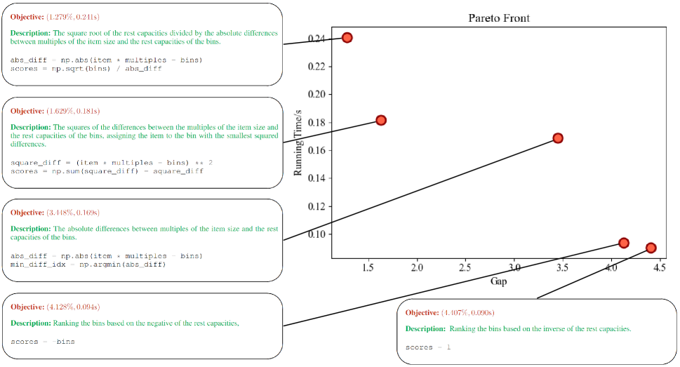
Figure 12: An illustration of MEoH heuristics on BPP.

In this section, Figure 12 showcases the heuristics developed by MEoH, featuring heuristic descriptions, corresponding code segments, and images in the objective space.

Specifically, these heuristics are designed to assign scores to bins based on the arriving items, subsequently arranging the items in bins with the highest scores.

Among these heuristics highlighted in Figure 12, three exhibit superior performance in terms of the optimal gap, leveraging advanced mathematical operators like absolute value and square root. Furthermore, in the case of the fast heuristic, the score is consistently set to a fixed value of $1$, which deviates from the intended description.

Given the integration of these heuristics into a greedy algorithm, the running time demonstrates low variance. Nevertheless, these MEoH-generated heuristics effectively balance the optimal gap and running time, enabling adaptability to diverse scenarios.

G.2 TSP

EoH Heuristics

The heuristic crafted by EoH, as illustrated in Figure 13, intricately incorporates advanced mathematical functions such as tanh alongside sophisticated parameters. It is noteworthy that this complex operation is executed within two nested for-loops, resulting in a computational complexity of $\mathcal{O}(n^{2})$.

Algorithm Description: Update the edge distances in the edge distance matrix by applying a genetic algorithm-inspired method, where the update is determined by a combination of edge count, distance, usage, and a customized genetic function to promote global exploration and improved convergence. ⬇ 1 2import numpy as np 3\pardef update_edge_distance(edge_distance, local_opt_tour, edge_n_used): 4updated_edge_distance = np.copy(edge_distance) 5\paredge_count = np.zeros_like(edge_distance) 6for i in range(len(local_opt_tour) - 1): 7start = local_opt_tour[i] 8end = local_opt_tour[i + 1] 9edge_count[start][end] += 1 10edge_count[end][start] += 1 11\paredge_n_used_max = np.max(edge_n_used) 12mean_edge_distance = np.mean(edge_distance) 13\parfor i in range(edge_distance.shape[0]): 14for j in range(edge_distance.shape[1]): 15if edge_count[i][j] > 0: 16score_factor = (np.tanh(edge_count[i][j]) / edge_count[i][j]) + (edge_distance[i][j] / mean_edge_distance) - (0.6 / edge_n_used_max) * edge_n_used[i][j] 17updated_edge_distance[i][j] += score_factor * (1 + edge_count[i][j]) 18\parreturn updated_edge_distance

Figure 13: The EoH heuristic with the best optimal gap on TSP.

FunSearch Heuristics

The heuristic formulated by FunSearch, as depicted in Figure 14, incorporates a logarithm operation base 2, Gaussian-distributed noise sampling, and intricate parameter configurations. It is worth noting that this heuristic only includes a single for-loop, indicating a computational efficiency that surpasses the aforementioned EoH heuristic.

⬇ 1 2def update_edge_distance(edge_distance: np.ndarray, local_opt_tour: np.ndarray, edge_n_used: np.ndarray) -> np.ndarray: 3num_nodes = edge_distance.shape[0] 4updated_edge_distance = np.copy(edge_distance) 5\pardecay_factor = 0.99 6\parfor i in range(num_nodes - 1): 7node_i, node_j = local_opt_tour[i], local_opt_tour[i + 1] 8\paredge_score = edge_distance[node_i, node_j] * np.log2((num_nodes - edge_n_used[node_i, node_j]) + 1) 9edge_score *= decay_factor ** edge_n_used[node_i, node_j] # Multiply by decay factor 10edge_score += np.random.normal(0, 0.1) # Add small noise 11\parupdated_edge_distance[node_i, node_j] = edge_score 12updated_edge_distance[node_j, node_i] = edge_score 13\parreturn updated_edge_distance

Figure 14: The FunSearch heuristic with the best optimal gap on TSP.

MEoH Heuristics

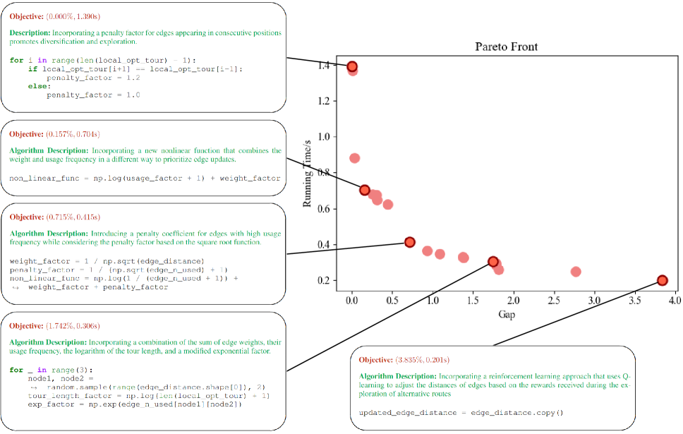
Figure 15: An illustration of MEoH heuristics on TSP.

In this section, the heuristics designed by MEoH are shown in Figure 15, showcasing $5$ representative heuristic descriptions along with corresponding code segments, and visual representations of all the heuristics in the objective space.

In this work, GLS is employed to solve TSP, and the heuristics are designed to update the edge distance to facilitate the perturbation in each iteration.

As shown in Figure 15, the designed heuristics leverage advanced mathematical operators including logarithm, square root, and exponential functions. Furthermore, for the fast heuristic, the edge distances remain unchanged, deviating from the original description due to the complexity of implementing Q-Learning.

These heuristics underscore the capability of our MEoH to strike a balance between the optimal gap and running time, allowing for effective adaptation to various scenarios.

References

- Agasiev and Karpenko (2017) Agasiev, T.; and Karpenko, A. 2017. The program system for automated parameter tuning of optimization algorithms. Procedia Computer Science, 103: 347–354.
- Applegate et al. (2006) Applegate, D.; Bixby, R.; Chvatal, V.; and Cook, W. 2006. Concorde TSP solver.
- Audet et al. (2021) Audet, C.; Bigeon, J.; Cartier, D.; Le Digabel, S.; and Salomon, L. 2021. Performance indicators in multiobjective optimization. European journal of operational research, 292(2): 397–422.
- Ausiello et al. (2012) Ausiello, G.; Crescenzi, P.; Gambosi, G.; Kann, V.; Marchetti-Spaccamela, A.; and Protasi, M. 2012. Complexity and approximation: Combinatorial optimization problems and their approximability properties. Springer Science & Business Media.
- Baxter et al. (1998) Baxter, I. D.; Yahin, A.; Moura, L.; Sant’Anna, M.; and Bier, L. 1998. Clone detection using abstract syntax trees. In Proceedings. International Conference on Software Maintenance (Cat. No. 98CB36272), 368–377. IEEE.
- Blot et al. (2016) Blot, A.; Hoos, H. H.; Jourdan, L.; Kessaci-Marmion, M.-É.; and Trautmann, H. 2016. MO-ParamILS: A multi-objective automatic algorithm configuration framework. In Learning and Intelligent Optimization: 10th International Conference, LION 10, Ischia, Italy, May 29–June 1, 2016, Revised Selected Papers 10, 32–47. Springer.
- Bozorg-Haddad, Solgi, and Loáiciga (2017) Bozorg-Haddad, O.; Solgi, M.; and Loáiciga, H. A. 2017. Meta-heuristic and evolutionary algorithms for engineering optimization. John Wiley & Sons.
- Burke et al. (2010) Burke, E. K.; Hyde, M.; Kendall, G.; Ochoa, G.; Özcan, E.; and Woodward, J. R. 2010. A classification of hyper-heuristic approaches. Handbook of metaheuristics, 449–468.
- Buse and Weimer (2009) Buse, R. P.; and Weimer, W. R. 2009. Learning a metric for code readability. IEEE Transactions on software engineering, 36(4): 546–558.
- Dang and De Causmaecker (2014) Dang, N. T. T.; and De Causmaecker, P. 2014. Motivations for the development of a multi-objective algorithm configurator. In International Conference on Operations Research and Enterprise Systems, volume 2, 328–333. SCITEPRESS.
- Deb et al. (2002) Deb, K.; Pratap, A.; Agarwal, S.; and Meyarivan, T. 2002. A fast and elitist multiobjective genetic algorithm: NSGA-II. IEEE transactions on evolutionary computation, 6(2): 182–197.
- Drake et al. (2020) Drake, J. H.; Kheiri, A.; Özcan, E.; and Burke, E. K. 2020. Recent advances in selection hyper-heuristics. European Journal of Operational Research, 285(2): 405–428.
- Dréo (2009) Dréo, J. 2009. Using performance fronts for parameter setting of stochastic metaheuristics. In Proceedings of the 11th Annual Conference Companion on Genetic and Evolutionary Computation Conference: Late Breaking Papers, 2197–2200.
- Fan et al. (2024) Fan, L.; Su, Z.; Liu, X.; and Wang, Y. 2024. Decomposition based cross-parallel multiobjective genetic programming for symbolic regression. Applied Soft Computing, 112239.
- Kaddour et al. (2023) Kaddour, J.; Harris, J.; Mozes, M.; Bradley, H.; Raileanu, R.; and McHardy, R. 2023. Challenges and applications of large language models. arXiv preprint arXiv:2307.10169.
- Kool, van Hoof, and Welling (2018) Kool, W.; van Hoof, H.; and Welling, M. 2018. Attention, Learn to Solve Routing Problems! In International Conference on Learning Representations.
- Li et al. (2024) Li, H.; Yang, X.; Wang, Z.; Zhu, X.; Zhou, J.; Qiao, Y.; Wang, X.; Li, H.; Lu, L.; and Dai, J. 2024. Auto mc-reward: Automated dense reward design with large language models for minecraft. In Proceedings of the IEEE/CVF Conference on Computer Vision and Pattern Recognition, 16426–16435.
- Liu et al. (2024) Liu, F.; Xialiang, T.; Yuan, M.; Lin, X.; Luo, F.; Wang, Z.; Lu, Z.; and Zhang, Q. 2024. Evolution of Heuristics: Towards Efficient Automatic Algorithm Design Using Large Language Model. In Forty-first International Conference on Machine Learning.
- Ma et al. (2024) Ma, P.; Wang, T.-H.; Guo, M.; Sun, Z.; Tenenbaum, J. B.; Rus, D.; Gan, C.; and Matusik, W. 2024. LLM and Simulation as Bilevel Optimizers: A New Paradigm to Advance Physical Scientific Discovery. arXiv preprint arXiv:2405.09783.
- Ma et al. (2023) Ma, Y. J.; Liang, W.; Wang, G.; Huang, D.-A.; Bastani, O.; Jayaraman, D.; Zhu, Y.; Fan, L.; and Anandkumar, A. 2023. Eureka: Human-level reward design via coding large language models. arXiv preprint arXiv:2310.12931.
- Mao et al. (2024) Mao, J.; Zou, D.; Sheng, L.; Liu, S.; Gao, C.; Wang, Y.; and Li, Y. 2024. Identify Critical Nodes in Complex Network with Large Language Models. arXiv preprint arXiv:2403.03962.
- Nasir et al. (2024) Nasir, M. U.; Earle, S.; Togelius, J.; James, S.; and Cleghorn, C. 2024. LLMatic: neural architecture search via large language models and quality diversity optimization. In Proceedings of the Genetic and Evolutionary Computation Conference, 1110–1118.
- Neamtiu, Foster, and Hicks (2005) Neamtiu, I.; Foster, J. S.; and Hicks, M. 2005. Understanding source code evolution using abstract syntax tree matching. In Proceedings of the 2005 international workshop on Mining software repositories, 1–5.
- Pearl (1984) Pearl, J. 1984. Heuristics: intelligent search strategies for computer problem solving. Addison-Wesley Longman Publishing Co., Inc.
- Pillay and Qu (2018) Pillay, N.; and Qu, R. 2018. Hyper-heuristics: theory and applications. Springer.
- Pillay and Qu (2021) Pillay, N.; and Qu, R. 2021. Automated Design of Machine Learning and Search Algorithms. Springer.
- Ramos et al. (2005) Ramos, I. C.; Goldbarg, M. C.; Goldbarg, E. G.; and Neto, A. D. D. 2005. Logistic regression for parameter tuning on an evolutionary algorithm. In 2005 IEEE congress on evolutionary computation, volume 2, 1061–1068. IEEE.
- Reinelt (1991) Reinelt, G. 1991. TSPLIB–A Traveling Salesman Problem Library. ORSA Journal on Computing, 3(4): 376–384.
- Reinelt (2003) Reinelt, G. 2003. The traveling salesman: computational solutions for TSP applications, volume 840. Springer.
- Ren et al. (2020) Ren, S.; Guo, D.; Lu, S.; Zhou, L.; Liu, S.; Tang, D.; Sundaresan, N.; Zhou, M.; Blanco, A.; and Ma, S. 2020. Codebleu: a method for automatic evaluation of code synthesis. arXiv preprint arXiv:2009.10297.
- Romera-Paredes et al. (2024) Romera-Paredes, B.; Barekatain, M.; Novikov, A.; Balog, M.; Kumar, M. P.; Dupont, E.; Ruiz, F. J.; Ellenberg, J. S.; Wang, P.; Fawzi, O.; et al. 2024. Mathematical discoveries from program search with large language models. Nature, 625(7995): 468–475.
- Schmidt and Lipson (2009) Schmidt, M.; and Lipson, H. 2009. Distilling free-form natural laws from experimental data. science, 324(5923): 81–85.
- Seiden (2002) Seiden, S. S. 2002. On the online bin packing problem. Journal of the ACM (JACM), 49(5): 640–671.
- Silver (2004) Silver, E. A. 2004. An overview of heuristic solution methods. Journal of the operational research society, 55: 936–956.
- Tang et al. (2014) Tang, K.; Peng, F.; Chen, G.; and Yao, X. 2014. Population-based algorithm portfolios with automated constituent algorithms selection. Information Sciences, 279: 94–104.
- van Stein and Bäck (2024) van Stein, N.; and Bäck, T. 2024. LLaMEA: A Large Language Model Evolutionary Algorithm for Automatically Generating Metaheuristics. arXiv preprint arXiv:2405.20132.
- Vasant (2012) Vasant, P. M. 2012. Meta-heuristics optimization algorithms in engineering, business, economics, and finance. IGI Global.
- Visheratin, Melnik, and Nasonov (2016) Visheratin, A. A.; Melnik, M.; and Nasonov, D. 2016. Automatic workflow scheduling tuning for distributed processing systems. Procedia Computer Science, 101: 388–397.
- Vladislavleva, Smits, and Den Hertog (2008) Vladislavleva, E. J.; Smits, G. F.; and Den Hertog, D. 2008. Order of nonlinearity as a complexity measure for models generated by symbolic regression via pareto genetic programming. IEEE Transactions on Evolutionary Computation, 13(2): 333–349.
- Voudouris, Tsang, and Alsheddy (2010) Voudouris, C.; Tsang, E. P.; and Alsheddy, A. 2010. Guided local search. In Handbook of metaheuristics, 321–361. Springer.
- Wang et al. (2024) Wang, H.; Skreta, M.; Ser, C.-T.; Gao, W.; Kong, L.; Streith-Kalthoff, F.; Duan, C.; Zhuang, Y.; Yu, Y.; Zhu, Y.; et al. 2024. Efficient Evolutionary Search over Chemical Space with Large Language Models. arXiv preprint arXiv:2406.16976.
- Xu, Hoos, and Leyton-Brown (2010) Xu, L.; Hoos, H.; and Leyton-Brown, K. 2010. Hydra: Automatically configuring algorithms for portfolio-based selection. In Proceedings of the AAAI Conference on Artificial Intelligence, volume 24, 210–216.
- Yao et al. (2024) Yao, Y.; Liu, F.; Cheng, J.; and Zhang, Q. 2024. Evolve Cost-aware Acquisition Functions Using Large Language Models. In International Conference on Parallel Problem Solving from Nature, 374–390. Springer.
- Ye et al. (2024) Ye, H.; Wang, J.; Cao, Z.; and Song, G. 2024. ReEvo: Large Language Models as Hyper-Heuristics with Reflective Evolution. arXiv preprint arXiv:2402.01145.
- Zeng et al. (2024) Zeng, J.; Li, C.; Sun, Z.; Zhao, Q.; and Zhou, G. 2024. tnGPS: Discovering Unknown Tensor Network Structure Search Algorithms via Large Language Models (LLMs). In Forty-first International Conference on Machine Learning.
- Zhang and Li (2007) Zhang, Q.; and Li, H. 2007. MOEA/D: A multiobjective evolutionary algorithm based on decomposition. IEEE Transactions on evolutionary computation, 11(6): 712–731.
- Zhang et al. (2024) Zhang, R.; Liu, F.; Lin, X.; Wang, Z.; Lu, Z.; and Zhang, Q. 2024. Understanding the Importance of Evolutionary Search in Automated Heuristic Design with Large Language Models. In International Conference on Parallel Problem Solving from Nature, 185–202. Springer.
- Zhang, Georgiopoulos, and Anagnostopoulos (2013) Zhang, T.; Georgiopoulos, M.; and Anagnostopoulos, G. C. 2013. S-Race: A multi-objective racing algorithm. In Proceedings of the 15th annual conference on Genetic and evolutionary computation, 1565–1572.
- Zitzler and Künzli (2004) Zitzler, E.; and Künzli, S. 2004. Indicator-based selection in multiobjective search. In International conference on parallel problem solving from nature, 832–842. Springer.
- Zitzler and Thiele (1998) Zitzler, E.; and Thiele, L. 1998. An evolutionary algorithm for multiobjective optimization: The strength pareto approach. TIK report, 43.