CREVE: An Acceleration-based Constraint Approach for Robust Radar Ego-Velocity Estimation

Abstract

Ego-velocity estimation from point cloud measurements of a millimeter-wave frequency-modulated continuous wave (mmWave FMCW) radar has become a crucial component of radar-inertial odometry (RIO) systems. Conventional approaches often perform poorly when the number of point cloud outliers exceeds that of inliers. In this paper, we propose CREVE, an acceleration-based inequality constraints filter that leverages additional measurements from an inertial measurement unit (IMU) to achieve robust ego-velocity estimations. To further enhance accuracy and robustness against sensor errors, we introduce a practical accelerometer bias estimation method and a parameter adaptation rule. The effectiveness of the proposed method is evaluated using five open-source drone datasets. Experimental results demonstrate that our algorithm significantly outperforms three existing state-of-the-art methods, achieving reductions in absolute trajectory error of approximately 53%, 84%, and 35% compared to them.

I INTRODUCTION

In recent years, millimeter-wave frequency-modulated continuous wave (mmWave FMCW) radio detection and ranging (radar) has gained significant attention in the field of robotics, particularly in applications focused on localization and navigation [1]. Due to its low cost, compact size, and ability to operate in all-weather conditions, radar emerges as a promising alternative to other perception sensors, such as cameras and light detection and ranging (LiDAR), which are often limited by poor lighting, illumination, and environmental factors [2, 3, 4, 5, 6]. Moreover, radar not only provides range and bearing information for objects of interest but also measures their Doppler velocity. In scenarios involving static objects, the ego-velocity of the sensor platform can be estimated [7]. This additional measurement is expected to further enhance localization performance, which, in turn, could lead to improved mapping accuracy.

Although static scene requirement is satisfied, ego-velocity estimation still remains a challenge. Due to the inherent characteristics of radar, outliers and noisy point cloud measurements resulting from multi-path signals and ghost targets make accurate estimation difficult [8]. Fig. 1 demonstrates an example of a system-on-chip (SoC) mmWave FMCW radar point cloud in an indoor scenario. The sparsity of the point cloud poses challenges for effective object detection and recognition. Additionally, the substantial variation in the Doppler velocities of objects (e.g., $-1.6253$ and $1.3753$ m/s in Fig. 1(a)) further complicates the estimation of the sensor’s velocity. This illustration also indicates that these challenges are amplified in confined environments, such as office spaces.

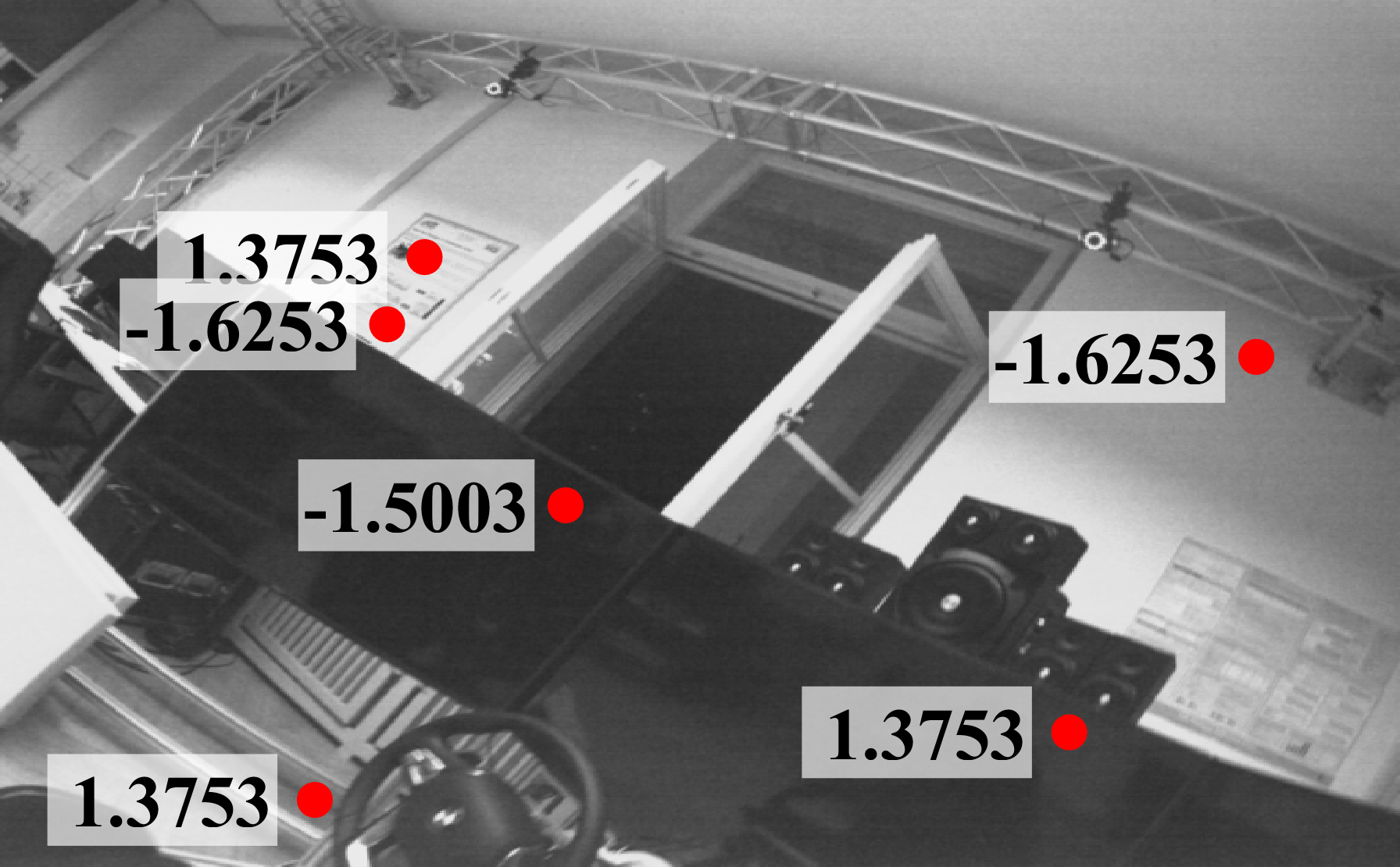
(a) MoCap Difficult.

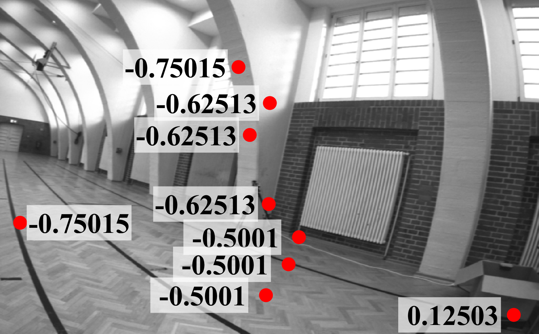
(b) Gym.

Figure 1: An example of 4D point cloud measurement from an mmWave FMCW radar of the open-source IRS dataset [9]. The radar’s 3D position points are projected onto a 2D image plane (red points), with each number indicating the corresponding 1D Doppler velocity.

To address the aforementioned problem, the implementation of a filtering technique or outlier removal algorithm is necessary. This preprocessing step is crucial for subsequent odometry [10] and mapping tasks [11]. However, a basic framework may prove insufficient in this context due to the presence of outliers. Generally, handling dynamic objects is considered more straightforward compared to dealing with radar ghost targets, given their arbitrary and unpredictable nature. To tackle this, most existing radar-only research focuses on consistently extracting static objects (e.g., the ground) [12] or on using previously estimated velocities to identify unusual estimation [13]. Nonetheless, these solutions may only be effective in specific situations and setups; for example, the radar must capture the ground for them to function properly. This requirement is often impractical for aerial systems or narrow indoor environments. Based on these observations, we believe that relying solely on spatial information and radar alone is insufficient. Consequently, integrating external sensors is essential and offers a promising approach to achieving robust estimation.

In this study, we present a framework that uses acceleration data estimated from an accelerometer as an inequality constraint to prevent incorrect radar-based ego-velocity estimation. Since acceleration represents the rate of change of velocity over time, this information allows us to establish boundary values for velocity estimation. In extreme scenarios where outliers, such as dynamic objects and ghost targets, vastly outnumber inliers, the estimation process is constrained to the acceleration surface. This approach ensures a robust estimation solution despite the presence of such outliers. Moreover, environmental factors such as scene changes or lack of features can be mitigated, as accelerometers are typically unaffected by these phenomena. Although our method requires an additional inertial measurement unit (IMU) sensor, such sensors are commonly available in most robotics applications. Notably, this proposed method complements our previous work in [14], which does not require accelerometers in odometry computation.

In summary, the contributions of this paper are as follows:

• We propose an acceleration-based Constraint method for robust Radar Ego-Velocity Estimation, termed CREVE, which addresses existing radar challenges. This framework functions as a submodule within a radar-inertial odometry (RIO) system.

• To enhance acceleration estimation from the accelerometer, we also introduce a practical bias calculation approach that leverages two consecutive constrained estimates of ego-velocity.

• Building on the work of [13], a practical adaptive parameter rule is developed to improve estimation accuracy by dynamically adjusting the range of the inequality constraint.

• A comprehensive analysis is conducted against existing state-of-the-art methods using the real-world IRS dataset [9]. The comparison uses root mean square error and absolute trajectory error as benchmarks.

II RELATED WORKS

II-A Radar Ego-Velocity Estimation

The use of radar for ego-motion estimation has been extensively explored in the literature through various methodologies. Broadly, these approaches can be categorized into two types: 1) estimating platform ego-velocity and subsequently fusing it with data from an IMU using a filter [15, 16, 14], and 2) estimating poses through scan matching algorithms [17, 18, 19]. The former approach has attracted more attention from researchers due to the challenges posed by the sparse and limited point clouds, particularly when SoC radar is employed. Moreover, when the focus is on odometry rather than mapping, the first approach requires only a single radar scan with a minimum of three points to estimate the platform’s ego-velocity, offering significant advantages [8]. One of the pioneering works in this field was presented by Kellner et al. in [20], where a single radar, combined with a random sample consensus/least squares (RANSAC/LSQ) estimator, was used to estimate the platform’s 2D ego-velocity. Building upon this foundation, the work in [21] employed multiple radars within the same pipeline. Doer and Trommer [10] further advanced this field by expanding the estimation from 2D to 3D ego-velocity with the modification of the RANSAC/LSQ model from a sinusoidal in [20] to a normalized position model of the point cloud. In a different fashion, Park et al. [22] utilized two perpendicular 2D radars to derive the 3D ego-velocity.

All of the methods mentioned above share a similar foundation, employing a basic RANSAC/LSQ workflow. However, this framework has empirically demonstrated poor performance in extreme environments, particularly in the $z$ direction, due to radar’s limited elevation angle resolution [8]. Jung et al. [23] improved upon this traditional approach by dividing the original workflow into a cascade of outlier removal processes for the $xy$ and $xz$ planes. Specifically, RANSAC/LSQ is first applied to the $x$ and $y$ axes, and the resulting inliers are then fed into a second RANSAC/LSQ, focused solely on the $x$ and $z$ directions. The authors claimed that this decoupling method improves accuracy in the $z$ direction, as the low-quality measurements from the $z$ axis do not affect the results from the $xy$ plane, thereby ensuring more reliable velocity estimation along the $x$ axis. However, this approach increases computational cost due to the use of two RANSAC algorithms. Alternatively, Štironja et al. [13] employed a different strategy by using a sliding window of previously estimated ego-velocity values to assess the anomaly of the current estimate. If the current outcome is identified to be unusual, it is deemed invalid and subsequently rejected. Nevertheless, this approach reduces the number of available radar measurements, which are already limited due to the radar’s low operational frequency (typically 10 Hz). This reduction may lead to divergence in a RIO system, where measurement updates are delayed over multiple steps To address this issue, we project the invalid estimation onto the constraint surface, rather than discarding them completely.

II-B Feature-based Outlier Removal

Unlike the previously discussed works, feature-based radar algorithms require a sufficient number of point clouds to compensate for the inherent sparsity of radar data and extract features of interest. In this regard, using a scanning radar is more suitable than a SoC type radar. Akarsh et al. [24] developed a neural network to transform radar point clouds into LiDAR-like point clouds for feature matching. Park et al. [25] employed phase correlation between two radar scans to infer relative motion. In [26], the authors applied the graduated non-convexity method to estimate ego-velocity and perform scan-to-submap matching. Lim et al. [27] further refined this outcome by introducing a rotation and translation decoupling method to remove outliers for scanning radar measurement. Alternatively, Chen et al. [12] combined point clouds from three SoC radars to generate a sufficient density of data points, enabling the extraction of ground features from the environment. It is important to note that all these studies primarily focus on ground vehicles in term of mapping. On the other hand, our study aims to explore odometry across various platforms (e.g., drones) that independent of the surrounding environment.

III PRELIMINARIES

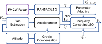
Figure 2: Block diagram overview of the proposed CREVE.

III-A Coordinate Frame and Mathematical Notations

In this article, the navigation (global) frame ${n}$ is defined as a local tangent frame fixed at the robot’s starting point, with axes aligned to the north, east, and downward. The IMU frame ${b}$ has axes pointing forward, right, and downward. The FMCW radar frame ${r}$ is oriented forward, left, and upward, with its origin at the center of the transmitter antenna. Superscripts denote the reference frame, subscripts indicate the target frame, and time indices are appended to subscripts for time-specific instances (e.g., $x_{b,k}^{n}$ represents a vector in ${b}$ at time step $k$, expressed in ${n}$). The direction cosine matrix $C_{b}^{n}$ transforms vectors from frame ${b}$ to frame ${n}$ and belongs to the special orthogonal group $SO(3)$.

In mathematical notation, $\mathbb{R}^{n}$ represents $n$-dimensional Euclidean space, while $\mathbb{R}^{m\times n}$ refers to the set of $m\times n$ real matrices. Scalars and vectors are written in lowercase (e.g., $x$), matrices in uppercase (e.g., $X$), with the transpose denoted as $X^{\top}$.

III-B RANSAC/LSQ Ego-Velocity Estimation

In this subsection, we provide briefly the iterative RANSAC/LSQ algorithm used to estimate 3D ego-velocity from a given set of radar point clouds. Most commercial mmWave FMCW radars produce a 4D point cloud for each spatial target, represented as $P_{i}=\begin{bmatrix}p_{i}\!\!&\!\!v_{D,i}\end{bmatrix}^{\top}$, where $p_{i}\in\mathbb{R}^{3}$ denote the position of the target $i$ expressed in $\{r\}$, and $v_{D,i}$ represents the corresponding 1D Doppler (radial) velocity. Given $\mathcal{P}_{k}=\{P_{i,k}|i=1,2,\ldots,N\}$ as a set of point cloud at the time instance $k$ with $|\mathcal{P}_{k}|\geq 3$ (where the operator $|.|$ returns the cardinality of the set, implying $N\geq 3$ or that the set contains at least 3 points), one can establish the following relationship [10]

$$\underbracket{\begin{bmatrix}-v_{D,1}\\ -v_{D,2}\\ \vdots\\ -v_{D,N}\end{bmatrix}=\begin{bmatrix}\bar{p}_{x,1}&\bar{p}_{y,1}&\bar{p}_{z,1}\\ \bar{p}_{x,2}&\bar{p}_{y,2}&\bar{p}_{z,2}\\ \vdots&\vdots&\vdots\\ \bar{p}_{x,N}&\bar{p}_{y,N}&\bar{p}_{z,N}\end{bmatrix}\begin{bmatrix}v_{x}^{r}\\ v_{y}^{r}\\ v_{z}^{r}\end{bmatrix}}_{y_{k}=H_{k}v_{k}^{r}}.$$ (1)

Here, $v_{k}^{r}\in\mathbb{R}^{3}$ is the radar velocity vector at time step $k$, and the direction vector $\bar{p}_{i}$ of target $i$ is obtained by normalizing $\bar{p}_{i}$, such that $\bar{p}_{i}=p_{i}/\|p_{i}\|_{2}^{\vphantom{2}}$. The estimate radar velocity $\hat{v}_{k}^{r}$ can be obtained by minimizing the squared $2$-norm loss function $\frac{1}{2}\big{\|}H_{k}\hat{v}_{k}^{r}-y_{k}\big{\|}_{2}^{2}$ . The well-known solution, given in [28], is $\hat{v}_{k}^{r}=\big{(}H_{k}^{\top}H_{k}\big{)}^{-1}H_{k}^{\top}y_{k}$.

The result discussed above does not account for outliers. To effectively handle outliers, the widely-used iterative RANSAC method [29] can be employed. Specifically, in each iterative, out of a fixed number of total iterations, three points from $\mathcal{P}_{k}$ are randomly select to compute a temporary estimate of $\hat{v}^{r}_{k}$. Inlier points are then determined by caclulating the absolute error between $y_{k}$ and $H_{k}\hat{v}_{r}^{k}$ for all points in $\mathcal{P}_{k}$, then comparing the error to a pre-determined threshold. Finally, the estimate $\hat{v}^{r}_{k}$ is refined by re-computing it using the inlier set.

IV METHODOLOGY

IV-A Overview

We begin by presenting an overview of our CREVE, as illustrated in the block diagram in Fig. 2. Our system adopts the conventional method from [10] with the state-of-the-art techniques outlines in [13]. To minimize computational complexity, the radar point cloud is initially processed using the traditional RANSAC/LSQ algorithm to extract an inlier set based on an initial estimate of ego-velocity. This inlier is subsequently utilized in the proposed inequality-constrained LSQ method. Meanwhile the initial estimate $\hat{v}_{k}^{r}$ is used to assess whether the result is anomalous, based on a moving window of size $M$ that containts previous velocity estimates. If the result falls outside the expected range, we incrementally tighten the inequality constraint to ensure robustness, rather than discarding it entirely as done in [13]. Next, to incorporate the acceleration constraint, the accelerometer measurements are compensated for both bias and gravity. In cases where an additional odometry filter is unavailable, the bias can be estimated from two consecutive radar-based ego-velocity estimations, while the attitude required for gravity compensation is derived from the gyroscope data.

IV-B Acceleration-constrained Least Squares

Given the rotation matrix and accelerometer bias estimation $\hat{b}_{a}$ at time instance $k$, the estimated acceleration expressed in the radar frame $\hat{a}_{f}^{r}$ can be calculated as

$$\hat{a}_{f}^{r}=C_{b}^{r}\big{(}\bar{f}^{b}-\hat{b}_{a}+C_{n}^{b}g^{n}\big{)}.$$ (2)

Here, $g^{n}$ represents the gravitational force vector, defined as $g^{n}=\begin{bmatrix}0&0&g\end{bmatrix}^{\top}$, where $g$ is the gravitational constant. The rotation matrix (extrinsic parameter) between the IMU and the radar $C_{b}^{r}$ is assumed to be given. For the sensor modeling, we adopt the model introduced in [14], which is given by $\bar{f}^{b}=C_{n}^{b}(a^{n}-g^{n})+b_{a}+n_{a}$. In this expression, $a^{n}$ and $n_{a}$ respectively signify the acceleration in the navigation frame and accelerometer noise.

Based on (2), we formulate the following linear programming (LP) problem —l—[] ~v_k^r ∈R^312 ∥H_k ~v_k^r - y_k ∥_2^2 ~v^r_k ≥( ^a^r_f, k - γ) Δt_r + ~v^r_k-1 ~v^r_k ≤( ^a^r_f, k + γ) Δt_r + ~v^r_k-1. In this relation, $\tilde{v}_{k}^{r}\in\mathbb{R}^{3}$ indicates the constrained ego-velocity estimation at time $k$, and $\Delta t_{r}$ is the radar time period. The LP above follows a standard form [30] and can be solved using various existing iterative methods. The inequality constraint is derived from the approximate relationship between average acceleration and velocity, given by $a^{r}_{k}=(v^{r}_{k}-v^{r}_{k-1})/\Delta t_{r}$. It is essential to recognize that these inequalities are subject to various sources of error, including attitude and bias estimation errors from (2) as well as discretization error. To take this issue into account, we introduce a pre-defined tuning parameter $\gamma\in\mathbb{R}^{3}$, which can be determined empirically. Incorporating $\gamma$ ensures that the nominal is adequately represented in the LP. Also, this parameter allows for the adjustment of the constraint range, providing flexibility to either tighten or loosen the constraints as needed.

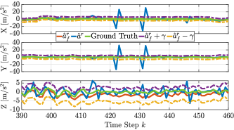
Figure 3: Our idea visualization using the IRS dataset [9], comparing the estimated $\hat{a}_{f}^{r}$ calculated from (2), MoCap ground truth, and average acceleration derived from $\hat{v}^{r}$. For this example, we used $\gamma=\begin{bmatrix}5\!\!&\!\!5\!\!&\!\!4\end{bmatrix}^{\top}$ (best viewed in color).

Our approach is visually demonstrated in Fig. 3. After compensating for bias and gravity, the estimated acceleration $\hat{a}^{r}$ provides valuable insight into the relationship between the current and previous velocity estimates. Additionally, the effectiveness of our proposed tuning parameter $\gamma$ is evident. With careful tuning, we can ensure that the ground truth acceleration consistently remains within the constraint boundaries. It is worth mentioning that we applied the standard method from [10] to produce this example, further supporting our claim that this method is not robust to outliers, even in a static environment, as evidenced by the peaks exceeding the constraint range.

IV-C Accelerometer Bias Estimation

In this subsection, we outline the process for estimating accelerometer bias using two consecutive radar ego-velocity measurements. According to [14], the relationship between the estimated body velocity expressed in navigation frame $\hat{v}_{b}^{n}$ and the constrained ego-velocity $\tilde{v}^{r}$ can be established as

$$\hat{v}_{b}^{n} =C_{b}^{n}C_{r}^{b}\tilde{v}^{r}-C_{b}^{n}\left[\bar{\omega}^{b}-\hat{b}_{g}\right]_{\!\times}p_{r}^{b},$$ (3)

where $\bar{\omega}^{b}$ is the raw gyroscope readings, $\hat{b}_{g}$ denotes gyroscope bias, and $p_{r}^{b}$ is the position of the radar relative to the $\{b\}$ frame. In this study, we assume that $\hat{b}_{g}$ and $p_{r}^{b}$ are known. These parameters can be obtained from a separated pre-processing step. For example, a coarse alignment algorithm, involving approximately 10 seconds of stationary data, can be used to estimate $\hat{b}_{g}$, while $p_{r}^{b}$ can be manually measured.

From this result and the previously described sensor model, one could yield the following equation

$$\hat{b}_{a}=\bar{f}^{b}+C_{n}^{b}\Bigg{(}g^{n}-\dfrac{\hat{v}_{b,k}^{n}-\hat{v}_{b,k-1}^{n}}{\Delta t_{r}}\Bigg{)}.$$ (4)

This calculation is practical and resembles that described in the previous subsection. The key difference is that, rather than compensating for bias and gravity to derive acceleration, (4) involves eliminating acceleration and gravity to directly estimate the bias. Combining these two methods appears to create a coupling relationship. However, we believe that by selecting $\gamma$ wisely, this coupling issue can be mitigated. In other words, all aforementioned error sources can be captured by our proposed parameter $\gamma$, which make the system more robust against to these errors. It is important to note that the bias estimation is influenced by the radar frequency, scaled by the factor $\Delta t_{r}$, which is typically around 10 Hz. This frequency can lead to substantial bias fluctuations. Since accelerometer bias varies slowly over time, we intentionally apply a low-pass filter to smooth the outcomes. Fig. 4 illustrates the performance of the bias estimation process described in (4).

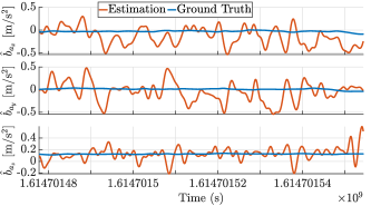
Figure 4: Accelerometer bias estimation of our CREVE, with a low-pass filter passband set to be 0.01 Hz.

IV-D Implementation

As mentioned earlier, our CREVE framework adopts the strategy outlined in [13], where anomalies of the current RANSAC/LSQ estimates are detected using a window of $M$ previous ego-velocity estimation. an estimate is considered invalid if the difference between the mean of the previous estimates and the newly estimated velocity norm exceeds a predefined threshold $T$. Additionally, if the difference between the last estimate and the current one is too large, indicating an acceleration above the threshold $a_{max}$, the estimate is also deemed invalid. In this case, we adjust the the inequality constraints in (IV-B) by slightly tightening them, i.e., by reducing $\gamma$. To achieve this adaptive adjustment, we select two value of $\gamma$, defined as $\gamma^{+}$ and $\gamma^{-}$, where each element of $\gamma^{+}$ is greater than the corresponding element of $\gamma^{-}$ ($\gamma^{+}_{i}>\gamma^{-}_{i}$ for $i=1,2,3$). Besides, we incorporate the a zero-velocity detection method from [10] to determine when the platform is stationary. A detailed, step-by-step implementation of our CREVE is provided in Algorithm 1.

Algorithm 1 CREVE

1:Initialize: $g^{n},\gamma^{+},\gamma^{-},T,a_{max}$, sliding window $W$, $Z$.

2:Performing coarse alignment for stationary motion $\rightarrow\hat{b}_{g},\hat{b}_{a}$.

3:for $k=1$ to $K$ do

4:    Computing the median $n$ of $v_{D,i}$ for all point cloud in $\mathcal{P}_{k}$.

5:    if $n<Z$ then

6:         Assigning $\hat{v}_{k}^{r}=0$.

7:    else

8:         Performing RANSAC/LSQ $\rightarrow\hat{v}_{k}^{r}$.

9:    end if

10:    if size of $W=M$ then

11:         Calculating $m=\frac{1}{M}\Sigma_{i=1}^{M}\|\hat{v}_{k-1}^{r}\|$.

12:         if $|m-\|\hat{v}_{k}^{r}\||<T$ and $\frac{1}{\Delta t_{r}}$$\|\hat{v}_{k}^{r}-\hat{v}_{k-1}^{r}\|<a_{max}$ then

13:             Assigning $\gamma=\gamma^{+}$.

14:         else

15:             Assigning $\gamma=\gamma^{-}$.

16:         end if

17:         Computing acceleration $\leftarrow$ (2).

18:         Solving the LP (IV-B) $\rightarrow\tilde{v}_{k}^{r}$.

19:         Calculating accelerometer bias $\leftarrow$ (4).

20:         Remove the oldest element of $W$.

21:         Appending $\tilde{v}_{k}^{r}$ to $W$.

22:    else

23:         Appending $\hat{v}_{k}^{r}$ to $W$.

24:    end if

25:end for

V NUMERICAL EXAMPLES

V-A Open-source datasets

To validate the proposed method (Ours), we used the renowned open-source IRS datasets provided by [9]. Specifically, we only selected five datasets that utilize a motion capture (MoCap) system to generate ground truth data for precise analysis. The selected datasets are named MoCap easy, medium, difficult, dark, and dark fast. We provide a brief overview of these datasets here; for a more detailed description of the experimental setup, we encourage readers to consult the original paper. These datasets were collected in an small laboratory room using a drone-based sensor platform equipped with a 4D FMCW radar (TI IWR6843AOP) and an IMU (Analog Devices ADIS16448). The IMU captures data at approximately 400 Hz, while the radar collects 4D point clouds at 10 Hz. On top of that, the radar offers a 120-degree field of view in both azimuth and elevation angles.

V-B Evaluation

We implemented our CREVE framework using MATLAB R2022b, running on a system equipped with an Intel i9-12900K CPU operating at 3.20 GHz. We compare the proposed method (Ours) with the following three state-of-the-art algorithms:

• REVE [10]: A standard RANSAC/LSQ-based framework for ego-velocity estimation.

• DeREVE [23]: A RANSAC/LSQ-based decoupling method designed to enhance the accuracy of velocity estimation along the $z$-axis.

• RAVE [13]: An extension of the REVE framework that incorporates mechanisms for detecting and rejecting anomalies in velocity estimation.

The parameters used in the experiments are as follows: gravitational constant $g=$ 9.81 m/s², $T=$ 7.5, $a_{max}=$ 10 m/s², $M=$ 5, $Z=$ 0.05. For the RANSAC algorithm, the success and outlier probability are set to 0.99 and 0.4, respectively. In the adaptive parameter settings, we use $\gamma^{+}=\begin{bmatrix}7.5\!\!&\!\!7.5\!\!&\!\!5\end{bmatrix}^{\top}$ and $\gamma^{-}=\begin{bmatrix}5\!\!&\!\!5\!\!&\!\!4\end{bmatrix}^{\top}$.

V-B1 Velocity Estimation

The $v^{r}$ estimation performance of all techniques are highlighted in Fig. 5. In typical scenarios, all of them exhibit comparable performance, with the exception of DeREVE, which displays some random peaks in its estimates. Conversely, RAVE consistently rejects anomalies, resulting in a discontinuous estimation. Interestingly, Ours also shows robustness against incorrect zero-velocity detection, as evidenced by the red box in the MoCap easy scenario.

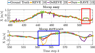
Figure 5: Comparison of ego-velocity estimation results across four investigated approaches using the MoCap easy and difficult datasets (best viewed in color).

(a)

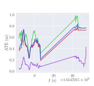
(b)

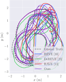
(c)

Figure 6: Odometry estimation results (easy) of the four methods compared to the MoCap ground truth using the toolbox [31]. The results are presented as: (a) $x$-$y$-$z$ position estimation comparison, (b) ATE comparison using Umeyama alignment, and (c) 2D $x$-$y$ trajectory comparison with the “x” marker denotes the end of the trajectory (best viewed in color).

TABLE I: Experimental results for 3D ego-velocity estimation, presented as RMSE for each $x$-$y$-$z$ axis. The table also includes the average computation time across all datasets and the number of rejections by the RAVE method.

Datasets	REVE [10] (0.007 s/loop)			DeREVE [23] (0.013 s/loop)			RAVE [13] (0.007 s/loop)				Ours (0.008 s/loop)
	$v_{x}$	$v_{y}$	$v_{z}$	$v_{x}$	$v_{y}$	$v_{z}$	$v_{x}$	$v_{y}$	$v_{z}$	Reject	$v_{x}$	$v_{y}$	$v_{z}$
Easy	0.120	0.069	0.086	0.178	0.111	0.292	0.103	0.067	0.086	4/766	0.066	0.038	0.110
Medium	0.158	0.085	0.262	0.310	0.178	0.350	0.155	0.078	0.128	7/719	0.133	0.071	0.105
Difficult	0.307	0.269	0.319	0.652	0.490	0.840	0.151	0.101	0.178	30/721	0.157	0.090	0.171
Dark	0.153	0.080	0.132	0.389	0.177	0.449	0.138	0.079	0.122	8/1264	0.132	0.078	0.118
Dark fast	0.197	0.248	0.196	0.517	0.478	0.832	0.117	0.076	0.129	8/643	0.113	0.089	0.122
Mean (m/s)	0.187	0.150	0.199	0.409	0.287	0.553	0.133	0.080	0.129	-	0.120	0.073	0.125
The bold numbers represent better results (the smaller number) and all values are rounded to three decimal digits.

TABLE II: Absolute trajectory error calculated with pos-yaw alignment [32], presented in terms of translation errors across five datasets for all considered approaches.

Datasets	REVE [10]	DeREVE [23]	RAVE [13]	Ours
Easy	0.596	0.664	0.562	0.167
Medium	0.357	1.047	0.259	0.148
Difficult	0.646	2.726	0.483	0.281
Dark	0.339	0.959	0.289	0.271
Dark Fast	0.531	2.018	0.207	0.292
Mean ATE (m)	0.494	1.483	0.360	0.232
The bold numbers represent better results (the smaller number).
All values are rounded to three decimal digits.

V-B2 Velocity Estimation Root Mean Square Error (RMSE)

Table I summarizes the RMSE between the ego-velocity estimates and the MoCap ground truth. Overall, our CREVE method outperforms the others across all experiments. Compared to the conventional approach (REVE), the proposed method reduces the RMSE by approximately 36% in the $x$-axis, 51% in the $y$-axis, and 37% in the $z$-direction, on average. In contrast, DeREVE demonstrates the lowest accuracy, while RAVE yields results comparable to those of CREVE. However, RAVE rejects 30 out of 721 radar measurements in the MoCap difficult experiments.

V-B3 Absolute Trajectory Error (ATE)

We calculate the odometry estimation directly from $v^{r}$ using attitude information, and utilize two well-known toolboxes [31, 32] to calculate the benchmark ATE. The results are summarized in Table II and illustrated in Fig. 6. Overall, Ours outperforms its competitors. Specifically, Fig. 6(b) suggests that CREVE achieves the smallest ATE in terms of minimum, maximum, and average ATE. Furthermore, Table II indicates that, on average, the proposed method reduces the ATE by approximately 53%, 84%, and 35% compared to REVE, DeREVE, and RAVE, respectively.

V-B4 Computation Time

We calculated the average time each method takes to process a set of radar point clouds across five datasets. Table I shows that DeREVE requires the longest processing time compared to the other methods, due to its use of double RANSAC/LSQ structure. In contrast, Ours has a processing time comparable to that of REVE and RAVE, with similar execution times for each iteration.

VI CONCLUSION

In this study, we have proposed CREVE, a robust radar ego-velocity estimation method that leverages acceleration from accelerometers as inequality constraints. The quantitative experimental results demonstrate that CREVE significantly outperforms existing state-of-the-art approaches. We have explicitly highlighted the strong relationship between radar and IMU for odometry purposes. As a submodule, the proposed method shows promising improvements in accuracy for a RIO system.

References

- [1] A. Venon, Y. Dupuis, P. Vasseur, and P. Merriaux, “Millimeter wave fmcw radars for perception, recognition and localization in automotive applications: A survey,” IEEE Transactions on Intelligent Vehicles, vol. 7, no. 3, pp. 533–555, 2022.
- [2] Y. Cheng, C. Pang, M. Jiang, and Y. Liu, “Relocalization based on millimeter wave radar point cloud for visually degraded environments,” Journal of Field Robotics, vol. 40, no. 4, pp. 901–918, 2023.
- [3] N. Yang, R. Wang, X. Gao, and D. Cremers, “Challenges in monocular visual odometry: Photometric calibration, motion bias, and rolling shutter effect,” IEEE Robotics and Automation Letters, vol. 3, no. 4, pp. 2878–2885, 2018.
- [4] D. Lee, M. Jung, W. Yang, and A. Kim, “Lidar odometry survey: recent advancements and remaining challenges,” Intelligent Service Robotics, vol. 17, no. 2, pp. 95–118, 2024.
- [5] S. H. Cen and P. Newman, “Precise ego-motion estimation with millimeter-wave radar under diverse and challenging conditions,” in 2018 IEEE International Conference on Robotics and Automation (ICRA), 2018, pp. 6045–6052.
- [6] K. Burnett, Y. Wu, D. J. Yoon, A. P. Schoellig, and T. D. Barfoot, “Are we ready for radar to replace lidar in all-weather mapping and localization?” IEEE Robotics and Automation Letters, vol. 7, no. 4, pp. 10 328–10 335, 2022.
- [7] M. A. Richards, J. Scheer, W. A. Holm, and W. L. Melvin, Principles of Modern Radar: Basic principles, ser. Radar, Sonar and Navigation. Institution of Engineering and Technology, 2010.
- [8] K. Harlow, H. Jang, T. D. Barfoot, A. Kim, and C. Heckman, “A new wave in robotics: Survey on recent mmwave radar applications in robotics,” arXiv preprint arXiv:2305.01135, 2023.
- [9] C. Doer and G. F. Trommer, “Radar visual inertial odometry and radar thermal inertial odometry: Robust navigation even in challenging visual conditions,” in 2021 IEEE/RSJ International Conference on Intelligent Robots and Systems (IROS), 2021, pp. 331–338.
- [10] C. Doer and G. F. Trommer, “An ekf based approach to radar inertial odometry,” in 2020 IEEE International Conference on Multisensor Fusion and Integration for Intelligent Systems (MFI), 2020, pp. 152–159.
- [11] J. Zhang, H. Zhuge, Z. Wu, G. Peng, M. Wen, Y. Liu, and D. Wang, “4dradarslam: A 4d imaging radar slam system for large-scale environments based on pose graph optimization,” in 2023 IEEE International Conference on Robotics and Automation (ICRA), 2023, pp. 8333–8340.
- [12] H. Chen, Y. Liu, and Y. Cheng, “Drio: Robust radar-inertial odometry in dynamic environments,” IEEE Robotics and Automation Letters, vol. 8, no. 9, pp. 5918–5925, 2023.
- [13] V.-J. Štironja, L. Petrović, J. Peršić, I. Marković, and I. Petrović, “Rave: A framework for radar ego-velocity estimation,” arXiv preprint arXiv:2406.18850, 2024.
- [14] H. V. Do, Y. H. Kim, J. H. Lee, M. H. Lee, and J. W. Song, “Dero: Dead reckoning based on radar odometry with accelerometers aided for robot localization,” in 2024 IEEE/RSJ International Conference on Intelligent Robots and Systems (IROS)., to be published.
- [15] C. Doer and G. F. Trommer, “Yaw aided radar inertial odometry using manhattan world assumptions,” in 2021 28th Saint Petersburg International Conference on Integrated Navigation Systems (ICINS), 2021, pp. 1–9.
- [16] Y. S. Kwon, Y. H. Kim, H. V. Do, S. H. Kang, H. J. Kim, and J. W. Song, “Radar velocity measurements aided navigation system for uavs,” in 2021 21st International Conference on Control, Automation and Systems (ICCAS), 2021, pp. 472–476.
- [17] S. H. Cen and P. Newman, “Radar-only ego-motion estimation in difficult settings via graph matching,” in 2019 International Conference on Robotics and Automation (ICRA), 2019, pp. 298–304.
- [18] J. Michalczyk, R. Jung, and S. Weiss, “Tightly-coupled ekf-based radar-inertial odometry,” in 2022 IEEE/RSJ International Conference on Intelligent Robots and Systems (IROS), 2022, pp. 12 336–12 343.
- [19] J. Michalczyk, R. Jung, C. Brommer, and S. Weiss, “Multi-state tightly-coupled ekf-based radar-inertial odometry with persistent landmarks,” in 2023 IEEE International Conference on Robotics and Automation (ICRA), 2023, pp. 4011–4017.
- [20] D. Kellner, M. Barjenbruch, J. Klappstein, J. Dickmann, and K. Dietmayer, “Instantaneous ego-motion estimation using doppler radar,” in 16th International IEEE Conference on Intelligent Transportation Systems (ITSC 2013), 2013, pp. 869–874.
- [21] D. Kellner, M. Barjenbruch, J. Klappstein, J. Dickmann, and K. Dietmayer, “Instantaneous ego-motion estimation using multiple doppler radars,” in 2014 IEEE International Conference on Robotics and Automation (ICRA), 2014, pp. 1592–1597.
- [22] Y. S. Park, Y.-S. Shin, J. Kim, and A. Kim, “3d ego-motion estimation using low-cost mmwave radars via radar velocity factor for pose-graph slam,” IEEE Robotics and Automation Letters, vol. 6, no. 4, pp. 7691–7698, 2021.
- [23] S. Jung, W. Yang, and A. Kim, “Co-ral: Complementary radar-leg odometry with 4-dof optimization and rolling contact,” in 2024 IEEE/RSJ International Conference on Intelligent Robots and Systems (IROS)., to be published.
- [24] A. Prabhakara, T. Jin, A. Das, G. Bhatt, L. Kumari, E. Soltanaghai, J. Bilmes, S. Kumar, and A. Rowe, “High resolution point clouds from mmwave radar,” in 2023 IEEE International Conference on Robotics and Automation (ICRA), 2023, pp. 4135–4142.
- [25] Y. S. Park, Y.-S. Shin, and A. Kim, “Pharao: Direct radar odometry using phase correlation,” in 2020 IEEE International Conference on Robotics and Automation (ICRA). IEEE, 2020, pp. 2617–2623.
- [26] Y. Zhuang, B. Wang, J. Huai, and M. Li, “4d iriom: 4d imaging radar inertial odometry and mapping,” IEEE Robotics and Automation Letters, vol. 8, no. 6, pp. 3246–3253, 2023.
- [27] H. Lim, K. Han, G. Shin, G. Kim, S. Hong, and H. Myung, “Orora: Outlier-robust radar odometry,” in 2023 IEEE International Conference on Robotics and Automation (ICRA), 2023, pp. 2046–2053.
- [28] D. Simon, Optimal state estimation: Kalman, H infinity, and nonlinear approaches. John Wiley & Sons, 2006.
- [29] M. A. Fischler and R. C. Bolles, “Random sample consensus: a paradigm for model fitting with applications to image analysis and automated cartography,” Commun. ACM, vol. 24, no. 6, p. 381–395, jun 1981. [Online]. Available: https://doi.org/10.1145/358669.358692
- [30] C. K. Liew, “Inequality constrained least-squares estimation,” Journal of the American Statistical Association, vol. 71, no. 355, pp. 746–751, 1976.
- [31] M. Grupp, “evo: Python package for the evaluation of odometry and slam.” https://github.com/MichaelGrupp/evo, 2017.
- [32] Z. Zhang and D. Scaramuzza, “A tutorial on quantitative trajectory evaluation for visual(-inertial) odometry,” in 2018 IEEE/RSJ International Conference on Intelligent Robots and Systems (IROS), 2018, pp. 7244–7251.