Asynchronous Fractional Multi-Agent Deep Reinforcement Learning for
Age-Minimal Mobile Edge Computing
Abstract
In the realm of emerging real-time networked applications like cyber-physical systems (CPS), the Age of Information (AoI) has merged as a pivotal metric for evaluating the timeliness. To meet the high computational demands, such as those in intelligent manufacturing within CPS, mobile edge computing (MEC) presents a promising solution for optimizing computing and reducing AoI. In this work, we study the timeliness of computational-intensive updates and explores jointly optimize the task updating and offloading policies to minimize AoI. Specifically, we consider edge load dynamics and formulate a task scheduling problem to minimize the expected time-average AoI. The fractional objective introduced by AoI and the semi-Markov game nature of the problem render this challenge particularly difficult, with existing approaches not directly applicable. To this end, we present a comprehensive framework to fractional reinforcement learning (RL). We first introduce a fractional single-agent RL framework and prove its linear convergence. We then extend this to a fractional multi-agent RL framework with a convergence analysis. To tackle the challenge of asynchronous control in semi-Markov game, we further design an asynchronous model-free fractional multi-agent RL algorithm, where each device makes scheduling decisions with the hybrid action space without knowing the system dynamics and decisions of other devices. Experimental results show that our proposed algorithms reduce the average AoI by up to compared with the best baseline algorithm in our experiments.
I Introduction
I-A Background and Motivations
Real-time embedded systems and mobile devices, including smartphones, IoT devices, and wireless sensors, have rapidly proliferated. This growth is driven by cyber-physical systems (CPS) applications such as collaborative autonomous driving [1], smart power grid [2], and intelligent manufacturing [3]. These applications generates vast amounts of data and requiring computationally intensive tasks that are progressively being processed closer to the mobile devices and edge nodes, rather than in the cloud. This surge in data and computation drives the needs for latency, reliability and privacy of processing on mobile devices or edge nodes. To address these intensive computational needs, mobile edge computing (MEC), also known as multi-access edge computing [4], has emerged as a workload architecture that distributes computational tasks and services from the network core to the network edge [5]. By enabling mobile devices to offload their computationally demanding tasks to nearby edge servers, MEC effectively reduces the processing delay associated with these tasks.
Additionally, there is another surge in the demand for real-time information updates across various CPS applications, such as ambient intelligence with IoT systems [6], autonomous driving [7] and industrial metaverse applications[8]. These applications require timely information updates. For instance, in industrial metaverse applications, users anticipate real-time virtual interactions along with actual industrial operations. In these real-time applications, the quality and precision of the user interactions hinge on information timeliness, rather than acquisition duration. For instance, critical applications such as high-resolution video crowdsourcing [9] and real-time collision warning [10] demand timely processing, yet local execution often leads to substantial latency or compromised quality. This need for data fresheness has led to the development of a new metric Age of Information (AoI) [11], which quantifies the elapsed time since the most recent data or computational results were received.
Although numerous prior studies on MEC have concentrated on minimizing delay (e.g., [12, 13]) without giving adequate attention to AoI, many real-time applications prioritize the freshness of status updates over mere delay reduction. Because status update freshness more accurately reflects the current relevance of information while delay does not directly reflect information timeliness. Here we highlight the substantial divergence between delay and AoI. Specifically, task delay only accounts for the duration from task generation to receipt of the task output by the mobile device. Thus, under less frequent updates (i.e. lower task generation frequency), task delays will naturally be smaller due to empty queues and reduced queuing delays, even though the freshness of updates cannot be assured. Conversely, AoI considers both task delay and the freshness of the output. This distinction between delay and AoI leads to a counter-intuitive phenomenon important for designing age-optimal scheduling policies: upon receiving each update, the mobile device may need to intentionally wait a certain duration before generating the subsequent new task [14]. In other words, the update frequency and the delay per task must be jointly optimized to minimize AoI for computationally intensive tasks. See [15] for further analysis of the tradeoffs between AoI and delay.
In this paper, we aim to answer the following questions:
Key Question.
How should mobile devices optimize their updating and offloading policies in real-time MEC systems in order to minimize AoI?
A few significant challenges of our paper include:
How to propose a fractional RL to combine the fractional optimization for AoI with RL? Optimizing AoI in MEC systems requires a sophisticated scheduling policy for mobile devices, which includes two fundamental decisions. First, the updating decision determines the optimal interval between task completion and the initiation of the subsequent task generation cycle. Second, the task offloading decision decides whether to offload a task to an edge server, and if so, selecting the optimal edge server. Prior work on MEC has investigated task offloading (e.g. [7, 16, 13, 17, 18, 19, 20, 21]) and some studies have considered AoI (e.g. [7, 16, 19, 20, 21]). However, they did not consider the fractional objective of AoI, which improves data timeliness while introduces significant complexity and instability for reinforcement learning (RL) due to its non-linear nature. Consequently, real-time MEC systems require a holistic approach that integrates both updating and offloading strategies and address the fractional AoI objective.
How should one deal with the adaption of fractional framework in multi-agent RL? Many MEC systems involve simultaneous decision-making processes among multiple mobile devices. Effectively addressing this multi-agent paradigm is imperative for tackling task scheduling and distributed computing. In these contexts, multi-agent reinforcement learning (MARL) has demonstrated considerable success [22]. However, the fractional nature of the AoI objective function introduces nonlinearity, adding complexity to its optimization within an MARL framework. Thus, the MARL framework faces challenges in optimizing the AoI objective.
How should one address the asynchronous decision problem in real-time MEC systems? Traditional MARL algorithms, like multi-agent deep deterministic gradient descent (MADDPG) [23] assume that agents make decisions synchronously. However, in multi-agent MEC systems, optimizing the AoI objective presents significant challenges. Furthermore, the inherent variability in task update and processing durations leads to asynchronous decision-making among agents, as transition times fluctuate throughout system operation. This fluctuating transitions aligns with the characteristics of semi-Markov games, where state transition intervals are stochastically determined rather than fixed. Consequently, addressing these challenges necessitates novel approaches that can effectively handle both the fractional objective and the asynchronous nature of agent interactions in MEC environments. Therefore, traditional MARL algorithms including QMIX [24] and MAPPO [25] would be inefficient to address the challenge of asynchronous control in mobile edge computing scheduling problem.
I-B Solution Approach and Contributions
In this paper, we aim to address the aforementioned key question and the associated challenges by designing multi-agent deep reinforcement learning (DRL) algorithms to jointly optimize task updating and offloading policies to minimize AoI in mobile edge computing systems. We propose a novel fractional RL framework that incorporates Nash Q-learning [26] with Dinkelbach’s approach for fractional programming as described in reference [20]. To handle the asynchronous decision-making scenario and hybrid action space, we further design a fractional multi-agent DRL-based algorithm.
Our main contributions are summarized as follows:
-
•
Joint Task Updating and Offloading Problem: We formulate the problem of joint task updating and offloading while accounting for multi-agent system and asynchronous control policies. To the best of our knowledge, this is the first work designing the joint updating and offloading multi-agent asynchronous policies for age-minimal MEC.
-
•
Fractional RL Framework: We consider the scenario of single-agent task scheduling and formulate a fractional RL framework that integrates RL with Dinkelbach’s method. This methodology is designed to adeptly handle fractional objectives within the RL paradigm and demonstrates a linear convergence rate.
-
•
Fractional MARL Framework: To address the fractional objective challenge in multi-agent scenario, we propose a novel fractional MARL framework. Our approach guarantees the existence of a Nash equilibrium (NE) in the proposed Markov game. Furthermore, we prove that our algorithm converges to this NE.
-
•
Asynchronous Fractional Multi-Agent DRL Algorithm: We propose a novel fractional asynchronous multi-agent DRL-based algorithm for multi-agent MEC systems. This algorithm addresses the asynchronous decision-making problem in semi-Markov games and the hybrid action space of offloading and updating decisions. Our approach aims to minimize AoI in MEC and approximate the Nash equilibrium. It extends two existing methods: the dueling double deep Q-network (D3QN) and proximal policy optimization (PPO). We enhance these methods with a fractional scheme and incorporate a recurrent neural network (RNN) which synthesizes information to evaluate other agents’ strategies.
-
•
Performance Evaluation: Our experimental evaluation demonstrates that asynchronous fractional multi-agent DRL algorithm outperforms established benchmarks across various metrics, showcasing its superior performance boost by up to 51.3%. Specifically, we observed that both the fractional module and the asynchronous mechanism contribute to enhancing the overall system performance.
II Literature Review
Mobile Edge Computing: Existing works have conducted various research questions in MEC, including resource allocation (e.g., [27]), service placement (e.g., [28]), proactive caching (e.g., [29]), and task offloading [30, 17, 31]. Among there areas, many works have proposed DRL-based approaches to optimize the task delay in a centralized manner (e.g., [32, 33]) while some existing works have proposed distributed DRL-based algorithms (e.g., [13, 34, 18]) which do not require the global information. Despite the success of these works in reducing the task delay, these approaches are NOT easily applicable to age-minimal MEC due to the challenges of fractional objective and asynchronous decision-making.
Multi-Agent RL in MEC: Multi-Agent RL has been widely adopted in multi-agent approaches with decentralized manners in MEC systems. Li et. al. proposed a decentralized edge server grouping algorithm and achieved NE by proving it be exact potential game [35]. Chen et al. addressed the task offloading in the information freshness-aware air-ground integrated multi-access edge computing by letting each non-cooperative mobile user behave independently with local conjectures utilizing double deep Q-network. Feng et al. utilized a gating threshold to intelligently choose between local and global observation and limit the information transmission for approximating Nash equilibrium in anti-jamming Markov game [36]. However, these MARL approaches have not considered the fractional objective when reaching NE.
Age of Information: Kaul et al. first introduced AoI in [11]. The majority of this line of work mainly focused on the optimization and analysis of AoI in queueing systems and wireless networks, assuming the availability of complete and known statistical information (see [37, 38, 39, 40, 41], and a survey in [42]). The above studies analyzed simple single-device-single-server models and hence did not consider offloading.
A few studies investigated DRL algorithm design to minimize AoI in various application scenarios, including wireless networks (e.g., [43]), Internet-of-Things (e.g., [44, 45]), autonomous driving[7], vehicular networks (e.g., [46]), and UAV-aided networks (e.g., [47, 48]). This line of work mainly focused on optimizing resource allocation and trajectory design. Existing works considered AoI as the performance metric for task offloading in MEC and proposed DRL-based approaches to address the AoI minimization problem. Chen et al. in [21] considered AoI to capture the freshness of computation outcomes and proposed a multi-agent DRL algorithm. However, these works focused on designing task offloading policy but did not jointly optimize updating policy. Most significantly, none of the aforementioned approaches have considered fractional RL, and hence they are unable to directly address the problem we focus on.
RL with Fractional Objectives: There is limited analysis on researches on RL with fractional objectives. Ren et. al. introduced fractional MDP [49]. Tanaka et. al. [50] further studied partially observed MDPs with fractional costs. However, these studies haven’t extended to RL framework. Suttle et al. [51] proposed a two-timescale RL algorithm for fractional cost optimization. However, this method requires fixed reference states in Q-learning updates, which can not be directly adapted in an asynchronous multi-agent environment.
Asynchronous Decision-Making MARL: Research on asynchronous decision-making in MARL is also limited. Chen et al. [52] proposed VarLenMARL in which each agent can have an independent time step with variable global system time length. Meanwhile, VarLenMARL maintains a synchronized delay-tolerant mechanism in which the agent can gather the padding data of the most up-to-date step of other agents. However, this approach becomes inefficient with a large number of agents and may neglect information from frequently deciding agents. Liang et al. [53] addressed these issues with ASM-PPO, which collected agent trajectories independently and trains using available agents at each time slot. But ASM-PPO could also lose track of the correct decision-making order when the decision-making frequencies vary significantly. Therefore, this algorithm cannot be adapted to our task scheduling problem, which involves high variability in agents’ decision-making.
III System Model
In this section, we present the system model for MEC. We first introduce the device and edge server model. We then define the AoI in our MEC setting and formulate the task scheduling problem within a semi-Markov game framework.
In this MEC system model, we consider mobile devices and edge servers respectively, as shown in Fig. 1. We denote the set of tasks be .
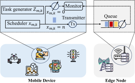
III-A Device Model
As shown in Fig. 1, each mobile device includes a task generator, a scheduler, a monitor, and a local processor. The generator produces computational tasks. The scheduler chooses to process them locally or offload to an edge server. After the edge server or local processor processes the task, the result is sent to the monitor and the generator then decides when to initiate a new task.
Generator: We consider a generate-at-will model, as in [14, 54, 55, 56, 57], i.e., the task generator of each mobile device decides when to generate the new task. Specifically, when task of mobile device is completed at , the task generator observes the latency of task and queue information of edge servers . It then decides on , i.e., the waiting time before generating the next task . We assume that edge servers share their load levels responding to the queries of mobile devices. Since a generator produces a new task after the previous task is finished, the queue length is less than or equal to , which incurs minimal signaling overheads. Let denote the updating action for task , i.e., and be the updating action space.
The time when the task is generated, can be calculated as . We note that the optimal waiting strategy for updating can outperform the zero-wait policy, implying that the waiting time is not necessarily zero and should be optimized for efficiency [14].
Scheduler: When the generator produces task at time , the scheduler makes the offloading decision denoted by with the queue information of edge servers111Under the system model in Section III, observing the queue lengths of edge servers is sufficient for mobile devices to learn their offloading policies. Under a more complicated system (e.g., with device mobility), mobile devices may need to observe additional state information, while our proposed fractional RL framework and DRL algorithm are still applicable with the extended state vector.. Let denote the action of task from mobile device . That is, . Let and denote the offloading action space and the task offloading policy of mobile device , respectively.
When task is processed locally on mobile device , we let (in seconds) denote the processing time of mobile device for processing task . The value of depends on the size of task and the real-time processing capacity of mobile device (e.g., whether the device is busy in processing tasks of other applications), which are unknown a priori. If mobile device offloads task to edge server , then let (in seconds) denote the latency of mobile device for sending task to edge server . The value of depends on the time-varying wireless channels and is unknown a priori. We assume that and are random variables that follow exponential distributions [58, 34, 59] and are independent across edge loads.
III-B Edge Server Model
When a mobile device offloads the task to edge server , the task is stored in the queue for processing, as shown in Fig. 1. We assume the queue operates in a first-come-first-served (FCFS) manner [42]. We denote as the queue lengths of all edge servers. Additionally, we assume that edge servers send their information of queue length upon request when a task is completed or when the waiting duration ends. 222Recall that a generator generates a new task only after the previous task has been processed, the queue length is less than or equal to . Thus, the information to be sent can be encoded in bits with minimal signaling overheads.
We denote (in seconds) as the duration that task of mobile device waits at the queue of edge server . Let (in seconds) denote the latency of edge server for processing task of mobile device . The value of depends on the size of task . We assume that is a random variable following an exponential distribution i.e., . Here, is the processing capacity (in GHz) of edge . Paramters and denotes the task size and task density of respectively. In addition, the value of depends on the processing time of the tasks placed in the queue (of edge server ) ahead of the task of device , where those tasks are possibly offloaded by mobile devices other than device . Thus, these offloading information cannot be observed by mobile device .
III-C Age of Information
For mobile device , the AoI at global clock [42] is defined by
| (1) |
where stands for the time stamp of the most recently completed task.
The overall duration to complete task is denoted by . Therefore,
| (2) |
We consider a deadline (in seconds) for all tasks. We assume that if a task is not finished within seconds, the task will be dropped [13, 60]. Meantime, the AoI keeps increasing until the next task is completed.
We define the trapezoid area associated with time interval :
| (3) |
where denotes the updating interval before generating next task . Based on (3), we can characterize the objective of mobile device , i.e., to minimize the time-average AoI of each device :
| (4) |
where is the expectation with respect to decisions made according to certain policies, which will be elaborated upon in the subsequent sections.
III-D Game Formulation
In MEC systems, mobile devices make updating and offloading decisions asynchronously due to variable transition times. These transition times, including waiting duration and latency, fluctuate based on scheduling strategies and edge workloads. Given that the current MARL framework is designed for synchronous decision-making processes, it is not suitable for application in this context. To characterize such asynchronous behaviors, we model the real-time MEC scheduling problem as a semi-Markov game (SMG). An SMG extends Markov decision processes to multi-agent systems with variable state transition times. Thus, this framework is able to address asynchronous decision-making in MEC systems by accommodating fluctuating transition times and allowing agents to act at different time points. The game is defined as , where is the set of agents (mobile devices in our system). A state can be expressed as , where denotes the decision indicators, specifying whether each mobile device needs to take offloading action , updating action or make no decisions. The state space is defined as .
The action space is defined as . Specifically, an action consists of its task updating action and task offloading action . We define the set of admissible triplets as . Let denote the collection of probability distributions over space . The transition function of the game is and the stochastic kernel determining the transition time distribution is . Additionally, denotes the initial state distribution.
We define policy space for semi-Markov game as , where each policy including both the updating and offloading policies of single mobile device . We define the expected long-term discounted AoI of mobile device as
| (5) |
where is a discount factor. We have the objective with the initial state under initial distribution . For simplicity, we drop the notation , which is by default unless stated otherwise in the following. Note that the discounted AoI form facilitates the application of AoI optimization within RL and MARL paradigms with discounted cost functions. Additionally, the discounted AoI (5) approximates the un-discounted AoI function (4) when approaches 1. We take the expectation over policy and the time-varying system parameters, e.g., the time-varying processing duration as well as the edge load dynamics. We define the Nash equilibrium for our minimization problem as follows.
Definition 1 (Nash Equilibrium).
In stochastic game , a Nash equilibrium point is a tuple of policies of cost functions such that for all we have,
| (6) |
For each mobile device , given the fixed stationary policies , the best response in our real-time MEC scheduling problem is defined as
| (7) |
Solving (7) is challenging due to the following reasons. First, the fractional objective introduces a major challenge in obtaining the optimal policy for conventional RL algorithms due to its non-linear nature. Second, the multi-agent environment introduces complex dynamics from interactions between edge servers and mobile devices. Third, the continuous time nature, stochastic state transitions, and asynchronous decision-making in SMG poses significant challenges in directly applying conventional game-theoretic methodologies.
In the following sections, we first analyze a simplified version of single-agent fractional RL framework. This framework establishes a robust theoretical foundation and serves as a benchmark for subsequent experiments. We then extend our theoretical analysis of our fractional framework to multi-agent scenarios, which is closer to SMG and piratical dynamics. Finally, we propose the fractional MADRL algorithm in asynchronous setting for SMG, which matches the practical dynamics of real-time MEC systems.
IV Fractional Single-Agent RL Framework
For fundamental theoretical analysis, we first consider the fractional single agent RL framework and design the fractional MDP. Then we propose fractional Q-learning algorithm with convergence analysis. We consider the problem as follows.
IV-A Single-Agent Problem Formulation
The objective for single-agent MEC system can be expressed as
| (8) |
where we focus on the policy of the agent alone compared with (7). We study the general fractional MDP framework and drop index in the rest of this section.
IV-B Dinkelbach’s Reformulation
To solve Problem (8), we consider the Dinkelbach’s reformulation. Specifically, we define a reformulated AoI in a discounted fashion:
| (9) |
Let be the optimal value of Problem (8). Leveraging Dinkelbach’s method [61], we have the following reformulated problem:
Lemma 1 ([61]).
Since for any and , is also optimal for the Dinkelbach reformulation. This implies that the reformulation equivalence is also established for our stationary policy space.
IV-C Fractional MDP
We then extend the standard MDP to a fractional form, laying the goundwork to more complex and practical setting in Markov game.
Definition 2 (Fractional MDP).
A fractional MDP is defined as , where and are the finite sets of states and actions, respectively; is the state transition distribution; and are the cost functions, is a discount factor, and denotes the initial global state distribution. We use to denote the joint state-action space, i.e., .
From Definition 2 and Lemma 1, Problem (8) has the equivalent Dinkelbach’s reformulation:
| (11) |
where we can see from Lemma 1 that satisfies
| (12) |
Note that Problem (11) is a classical MDP problem, including an immediate cost . Thus, we can apply a traditional RL algorithm to solve such a reformulated problem, such as Q-Learning or its variants (e.g., SQL in [62]).
However, the optimal quotient coefficient and the transition distribution are not known a priori. Therefore, we design an algorithm that combines fractional programming and reinforcement learning to solve Problem (11) for a given and seek the value of . To achieve this, we start by introducing the following definitions.
Given a quotient coefficient , the optimal Q-function is
| (13) |
where is the action-state function that satisfies the following Bellman’s equation: for all ,
| (14) |
where is a concise notation for . In addition, we can further decompose the optimal Q-function in (13) into the following two parts: and, for all ,
| (15) | ||||
| (16) |
IV-D Fractional Q-Learning Algorithm
In this subsection, we present a Fractional Q-Learning (FQL) algorithm (see Algorithm 1). The algorithm consisting of an inner loop with episodes and an outer loop. The key idea is to approximate the Q-function using in the inner loop, while iterating over the sequence in the outer loop.
A notable innovation in Algorithm 1 is the design of the stopping condition, which ensures that the uniform approximation errors of shrink progressively. This allows us to adapt the convergence proof from [61] to our inner loop, while proving the linear convergence rate of in the outer loop. Importantly, this design does not increase the time complexity of the inner loop.
We describe the details of the inner loop and the outer loop procedures of Algorithm 1 in the following:
-
•
Inner loop: For each episode , given a quotient coefficient , we perform an (arbitrary) Q-Learning algorithm (as the Speedy Q-Learning in [62]) to approximate function by . Let denote the initial state of any arbitrary episode, and for all . We consider a stopping condition
(17) where is the error scaling factor. This stopping condition ensures the algorithm being terminated in each episode with a bounded uniform approximation error: Operator is the supremum norm, which satisfies . Specifically, we obtain , , and , which satisfy,
(18) -
•
Outer loop: We update the quotient coefficient:
(19) which will be shown to converge to the optimal value .
IV-E Convergence Analysis
We present the time complexity analysis of inner loop and the convergence results of our proposed FQL algorithm (Algorithm 1) as follows.
IV-E1 Time Complexity of the inner loop
IV-E2 Convergence of FQL algorithm
We then analyzing the convergence of FQL algorithm:
Theorem 1 (Linear Convergence of Fractional Q-Learning).
If the uniform approximation error holds with for some and for all , then the sequence generated by Algorithm 1 satisfies
| (20) |
That is, converges to linearly.
While the convergence proof in [61] requires to obtain the exact solution in each episode, Theorem 1 generalizes this result to the case where we only obtain an approximated (inexact) solution in each episode. In addition to the proof techniques in [61] and [62], our proof techniques include induction and exploiting the convexity of . We present a proof sketch of Theorem 1 in Appendix B .
V Fractional Multi-Agent RL Framework
To extend our fractional framework from the single-agent scenario to the multi-agent one, we propose a fractional Markov game framework in this section. We first introduce a Markov game for our task scheduling problem. We then introduce a fractional framework consisting of fractional sub-games to address the challenge of the fractional objective. Finally, we propose a corresponding MARL scheme and prove its convergence to the Nash equilibrium.
V-A Markov Game Formulation
We study our problem in the context of multi-agent and introduce the framework of task scheduling Markov game.
The task scheduling Markov game can be defined as: where is the number of agents, and represent the state space and action space, respectively, denotes the state transition probability, is discounted factor, and denotes the initial state distribution.
We define the instant fractional costs at task of mobile device as
| (21) | |||
| (22) |
Following the definition of discounted AoI in (5), we define the fractional long-term discounted cost for mobile device as
| (23) |
where be policies of mobile device and other agents that determine actions to execute, and is the expectation regarding transition dynamic given stationary control policy . Note that (23) approximates the un-discounted function when approaches 1 [63]. Specifically, an NE is a tuple of policies of game . For each mobile , given the fixed stationary policies , the fractional objective can be expressed as:
| (24) |
Lemma 2 guarantees the existence of a Nash equilibrium in our game .
Lemma 2.
By [64], for the multi-player stochastic game with expected long-term discounted costs, there always exist a Nash equilibrium in stationary polices, where the probability of taking an action remains constant throughout the game.
V-B Fractional Sub-Game
To deal with the fractional objective (24) with for Nash equilibrium, we reformulated our game into iterative fractional sub-games based on Dinkelbach method[61] in the this subsection. In the context of the proposed game , we utilize Dinkelbach’s reformulation [61] to tackle the challenge posed by the fractional objective. We then introduce an iterative fractional sub-game method for the game .
We first define sub-game given fractional coefficients for fractional sub-games as follows.
Definition 3 (Fractional Sub-Game).
The fractional sub-game is defined as , where are the set of fractional coefficients. Each is specific to mobile device m. These coefficients are used in the optimization process for the fractional sub-game.
The fractional discounted cost value functions of sub-game is denoted as , then the fractional cost function of mobile device can be defined as
| (25) |
where are the global state and action at task . The objective of each mobile device of sub-game is to device the best response that minimize its own cost value with fixed policies of other agents for any given global system state is obtained as
| (26) |
Lemma 2 ensures the existence of an NE in our game . For brevity, we denote the optimal state-value function as , where is the NE of sub-game .
We will show the convergence of and the equivalence between fractional sub-games and game in the subsequent subsections.
V-C Fractional Nash Q-Learning Algorithm
We now present a Fractional Nash Q-Learning (FNQL) algorithm in Algorithm 2. This algorithm includes 1) an inner loop to approximate Nash function and obtain Nash equilibrium of sub-game , and 2) an outer loop to iterate and reach the convergence of . The key idea is to iterate sub-game and ultimately attain the Nash equilibrium of Markov game when converges.
V-C1 Inner Loop
Following [65], we first define the Nash operator for the mapping from a cost function to its value with NE:
Definition 4.
Consider a collection of M functions that can achieve a Nash equilibrium , denoted as . We introduce the Nash operator , which maps the collections of functions into the values with their corresponding Nash equilibrium values as
| (27) |
where satisfies
| (28) |
For sub-game , the optimization of best response (26) utilize an instant cost, given by . To solve this optimization, we apply the traditional MARL algorithm Nash Q-learning[26]. We define the Nash Q-function with as:
| (29) |
where we denote , is a concise notation for . In the inner loop, we update Q-function of mobile device at task by
| (30) |
where is the learning rate.
Then, let be the collection of Q-functions of mobile devices. As in [65], . The Nash-Bellman equation can be expressed as
| (31) |
We define , as follows
| (32) | |||
| (33) |
where specifically, and . Then we have .
For each sub-game , we perform the fractional Nash Q-Learning algorithm to obtain the optimal value function . Each episode terminates when the sub-game achieves Nash equilibrium.
V-C2 Outer loop
The outer loop implements the Nash generation following the framework of Dinkelbach method [61]. After achieving the NE of sub-game , we update the quotient coefficient in line 9 of Algorithm 2 as :
| (34) |
We repeat this process until converges. The convergence of is discussed in the following subsection.
V-D Convergence Analysis
We proceed to build the equivalence between the optimization with fractional sub-games iteration proposed above and the original game .
We are ready to present the convergence results of our proposed fractional Nash RL algorithm (Algorithm 2) for the game . This facilitates us to adapt the convergence proof in [61] to our setting.
We first examine the existence of an equivalent condition of reaching NE between the Markov game and the fractional sub-game with the following lemma:
Lemma 3.
For each mobile device , there exists , such that at the NE of sub-game .
The proof of Lemma 3 mainly utilizes the Brouwer fixed point theorem. See Appendix C for detailed proof. We then analyze the equivalence for reaching NE between the Markov game and the fractional sub-game :
Lemma 4.
Markov game attains Nash equilibrium strategies if and only if sub-game achieves the Nash equilibrium and .
The proof Lemma 4 established upon the result of Lemma 3. See Appendix D for proof. We define two conditions when sub-game attains an NE as:
Definition 5 (Global optimum).
A strategy profile is a global optimal point if, for all agents , the following inequality holds:
| (35) |
Definition 6 (Saddle Point).
A strategy profile is a saddle point if, for all agents , the following inequalities holds:
| (36) | |||
| (37) |
Assumption 1.
For each sub-games in training, the Nash equilibrium of sub-game is recognized either as Condition A the global optimum or Condition B a saddle point expressed.
Assumption 1 imposes a relatively stringent constraint. However, we empirically show that this constraint may not be a necessary condition for the convergence of the learning algorithm. This observation aligns with the empirical findings reported by Hu and Wellman [26]. Moreover, this assumption is widely adopted in theoretical frameworks analyzing MARL[66], and is similarly applied in other MARL methodologies, such as Mean-field MARL [67] and Friend-or-Foe Q-learning [68] as well.
Choose . Then for any , we have . Define a compact and convex set and mapping of in Algorithm 2 as:
| (38) |
We present the definition of contraction mapping and the contraction mapping of as follows.
Definition 7.
(Contraction Mapping) Let be a metric space and be a mapping. The mapping is a contraction mapping if there exists such that:
| (39) |
Theorem 2.
(Contraction Mapping of )
VI Asynchronous Fractional Multi-Agent DRL Algorithm
In previous section, we has proposed the fractional Nash Q-learning algorithm to deal with the fractional objective in Markov games. However, when considering scheduling problem of MEC formulated in semi-Markov game, the tasks from mobile devices finish asynchronously and synchronized decision-making and training are inefficient. Thus, in this section, we first introduce an asynchronous trajectory collection mechanism named RNN-PPO and then propose an asynchronous fractional multi-agent DRL framework for solving Problem (7) in semi-Markov game.
VI-A Asynchronous Trajectory Collection Mechanism
To train MARL algorithms, we collect trajectories from agents, including global states, local observations, actions, and costs. However, traditional MARL algorithms like MADDPG [23] and MAPPO require synchronous joint information from all agents at each time step, making them unsuitable for asynchronous settings. VarlenMARL [52] addresses this by allowing variable-length trajectories, but it still struggles to fully utilize agent interactions in asynchronous environments.
Our method introduces a novel asynchronous trajectory collection mechanism. It collects agent trajectories based on a global task, asynchronously aggregating historical decision-making at local task, including global states and other agents’ strategies. This approach better leverages agent interactions and asynchronous collaboration. To illustrate, consider a mobile device performing task , where is the global state, the action, the cost, and the history at local timestamp and global clock . We compare our asynchronous mechanism with traditional MARL and VarlenMARL using two agents.
Traditional MARL algorithms collect the joint data of all agents at the each time step. That is, the joint trajectory collected is
.

(a)
(b)
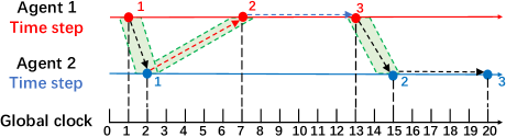
Since asynchronous decision-making events cannot be collected synchronously, VarlenMARL [52] let agents collect their own trajectories with its own data combined with the latest padded data from other agents. Let be the initial trajectory of agent . The trajectories shown in Figure 2(a) of Agent 1 and Agent 2 are
However, we observe that when agents’ task timelines are significantly unsynchronized, Agent 2’s information at global task 7 cannot be used as padding, disrupting the training process.
Our proposed trajectory collection mechanism as shown in Fig. 2(b) requires agents to collect their actions asynchronously in execution time order. We define time-aggregating information as , which is updated as , where function is time-aggregating function and is the latest state-action tuple. Additionally, the agent collects the time-aggregating information at global clock . In this way, agents are able to evaluate their state values and Q values more accurately with both observations and aggregated information from previous actions of all agents. The collected trajectory as shown in Fig. 2(b) is as follows:
Our proposed trajectory collection mechanism allows agents to collect memories asynchronously while leveraging time-aggregated information from past events in actual task order during both execution and training.
VI-B Cost Module
As in the proposed fractional MARL framework in section 5, we consider a set of episodes and introduce a quotient coefficient for episode . Let denote the set of updating and offloading strategies of mobile device in iteration with tasks, where superscript ‘H’ refers to ‘hybrid’. At task step ,333Here, step refers to the updating and offloading processes as well as the training process associated with task . a cost is determined and sent to the DRL modules. This process corresponds to the sub-game of the proposed fractional RL framework and is defined based on (26):
| (40) |
where stands for the area of a trapezoid in (3) and and are the duration of task and the time that the task generator waits to produce the next task , respectively. Note that is a function of , and is a function of . The cost module keeps track of or equivalently and for all across the training process.
Finally, at the end of each episode , the cost module updates as:
| (41) |
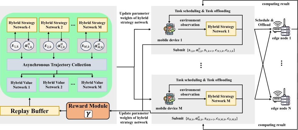
VI-C Fractional Asynchronous Multi-Agent DRL Framework
We present a fractional asynchronous multi-agent DRL-based framework (FA-MADRL) to achieve Nash equilibrium for Problem (7) and hybrid action space as shown in Figure 3. We train hybrid strategy networks for each mobile device which will updated to the mobile device to make decisions of hybrid actions444We centrally train the hybrid networks in a trusted third-party.. We adapt our asynchronous trajectory collection mechanism which synthesize the time-aggregating data to take use of state-action pairs from other agents and history events to interactive with other agents and history context when training with hybrid value networks. Adapting this mechanism in recurrent network, we apply our trajectory collection mechanism both on D3QN for discrete action space and proximal policy optimization (PPO) for continuous action space to deal with the task offloading and updating processes which are illustrated in Appendix F in detail. In addition, we design a cost module of for our fractional loops to ensure the overall convergence to Nash equilibrium.
VII Performance Evaluation
We evaluate our fractional multi-agent framework with experiments where 20 mobile devices learning their policies with interactive information. Basically, we follow the experimental settings of [13, Table I] and present details in Appendix G.
VII-A Baseline
We denote the proposed Fractional Multi-Agent DRL as FMADRL, which is compared with several benchmark methods.
-
•
Random: The updating and offloading decisions are randomly scheduled within action space.
-
•
Non-Fractional DRL (denoted by Non-F. DRL): This benchmark let each mobile devices learn their hybrid DRL algorithms individually without fractional scheme and multi-agent techniques. It exploits the same D3QN network as our proposed algorithm to generate discrete action for offloading decisions and PPO with continuous action for updating decisions. In comparison to our proposed fractional framework, this benchmark is non-fractional and is lack of the trajectory collection mechanism. It approximates the ratio-of-expectation average AoI by an expectation-of-ratio expression: This approximation to tackle the fractional challenge tends to cause large accuracy loss.
-
•
Fractional DRL (denoted by F. DRL): This benchmark adapts our fractional framework to the algorithm Non-F. DRL and is used to express the effectiveness of our proposed fractional technique. This benchmark exploits the same fractional framework as our proposed algorithm but the trajectory collection mechanism to deal with the asynchronous issue is missing.
-
•
H-IPPO: Independent proximal policy optimization [69] with hybrid action spaces for the updating and offloading decisions for the updating and offloading decisions.
-
•
H-MAPPO: Multi-agent proximal policy optimization [70] with hybrid action spaces for the updating and offloading decisions for the updating and offloading decisions.
-
•
VarlenMARL: VarLenMARL[52] adopts independent time step with variable length for each agent and leverages the synchronized delay-tolerant mechanism to improve performance as mentioned in Section 2 and 6.
-
•
Fractional Asynchronous Multi-Agent DRL (denoted by F. A. MADRL): Proposed algorithm adapts both the fractional scheme to approximate the averaged AoI and the trajectory collection mechanism to account for the information from history records and other agents.

(a) (b)
VII-B Experimental Results
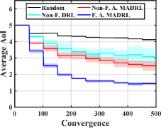
We empirically evaluate the convergence of our proposed algorithms and compare their performance against baselines. We systematically conduct experiments on edge capacity, drop coefficient, task density, mobile capacity, processing variance, and number of agents with proposed algorithms and baselines. Convergence: Fig. 4 demonstrates the convergence of Non-F. DRL and proposed F.DRL and F. A. MADRL algorithms. In contrast to non-fractional methods, our proposed methods consist of not only the convergence of target metric but also the fractional coefficient and they are supposed to converges at the same time. As a result, the convergence curve of averaged AoI may sometimes change non-monitonically. In Fig. 4(a), F. DRL and F. A. MADRL converges after about 300 episodes. Regarding to the converged averaged AoI, F. A. MADRL outperforms Non-F. DRL by 53.7%. The performance gap between DP and Frac. DP illustrates the necessity of our proposed fractional framework. The difference between Frac. DP and F. A. MADRL shows the significance of proposed trajectory collection.


(a) (b) (c)
(d) (e) (f)
(e) processing variances, (f) number of agents.
Edge Capacity: In Fig. 5(a), we evaluate different processing capacities of edge nodes. With the asynchronous trajectory collection scheme, Non-F. A. MADRL reduces the average AoI about 29.7% on average. Moreover, The proposed F. A. MADRL algorithm archieves lower average AoI consistently compared to other benchmarks without considering fractional AoI and asynchronous settings. it reduces the average AoI up to 36.0% compared to MAPPO at 55 GHz. This further shows that better design for asynchronous setting can archieves better performance when there exist relatively more edge capacity capabilities to exploit.
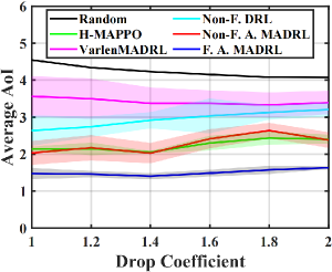
Drop Coefficient: Fig. 5(b) considers different drop coefficients which are the ratios of drop time to the average duration of task processing. Although the average AoI of random scheduling shrinks as the drop coefficient gets large, the performance of other RL techniques have’t shown a clear trend. This indicates that the updating policy may serves the function of dropping mechanism. Bescides, our proposed F. A. MADRL approach archives about 32.9% less average AoI compared against MAPPO on average.
Task Density: In Fig. 5(c), we evaluate AoI performance under different task densities, which determine the overall task loads and expected processing time on both mobile devices and edge nodes. Our proposed F. A. MADRL algorithm outperforms all the other benchmarks. Specifically, F. A. MADRL reduces the average AoI by up to 41.3% and 63.5% compared to MAPPO and Non-Fractional DRL at 15 Gigacycles per Mbits, respectively. Meanwhile, Non-F. A. MADRL outperforms Non-F. DRL by 17.5% on average, which demonstrates the effect of our asynchrnous trajectory collection scheme.
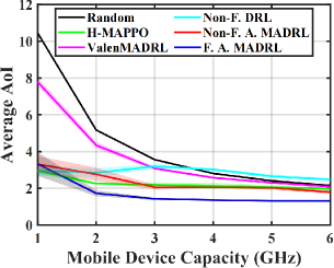
Mobile Capacity: In Fig. 5(d), we consider different mobile device capacities, where our proposed F. A. MADRL algorithm reduces average AoI by 39.1% on average compared with Non-F. DRL algorithm. We can see that performance gaps between algorithms narrow when mobile device capacity is very high because at that time mobile devices process their tasks process their tasks locally at most times and the effect of scheduling shrinks. And it seems that Non-F. DRL tends to offload tasks to edge nodes and perform badly when mobile device capacity is high and the performance is relatively steady when the capacity of mobile devices change.
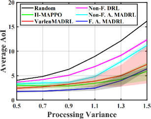
Processing Variance: Fig. 5(e) considers performance of algorithms under different variances of processing time which is evaluated as lognormal distribution in this part of experiment. It demonstrates that proposed F. A. MADRL algorithm shows significant performance advantage when the variance is relatively high at 1.1 and 1.3 by over 18%, which indicates that our asynchronous trajectory collection mechanism works well when decision steps of mobile devices vary dramatically over time.
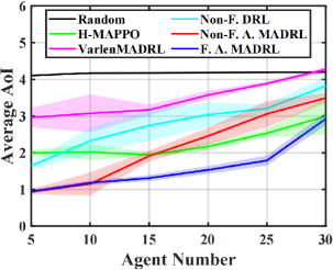
Number of Agents: Fig. 5(f) considers different amounts of agents or mobile devices with same edge nodes. In this case, the proposed F. A. MADRL algorithm achieves significant performance advancement up to 52.6% compared with MAPPO. And the performance gap between our proposed algorithm and benchmarks narrows when the number of mobile devices are very low or very high. Because in these cases either the computing capabilities of edge nodes or mobile devices themselves are abundant where the scheduling strategies don’t matter that much.
VIII Conclusion
In this paper, we proposed three schemes to tackle the computational task scheduling (including offloading and updating) problem in a semi-Markov game for age-minimal MEC. First, we propose a fractional RL framework to address the fractional objective in single-agent setting. Second, to address the fractional objective and load dynamics in multi-agent, we proposed a Nash fractional RL scheme with theoretical convergence to Nash equilibrium. Third, to settle the asynchronous multi-agent problem of mobile edge computing in semi-Markov game, we further proposed a trajectory collection mechanism with RNN network. Evaluation results indicates that both proposed fractional scheme and trajectory collection scheme significantly improve the performance for average AoI, validating the effects of the two techniques. In future works, apart form AoI, it’s worth concerning the energy consumption and security satisfaction at the same time, whose problem could be in fractional form as well.
References
- [1] D. Katare, D. Perino, J. Nurmi, M. Warnier, M. Janssen, and A. Y. Ding, “A survey on approximate edge ai for energy efficient autonomous driving services,” IEEE Communications Surveys & Tutorials, 2023.
- [2] Z. Xu, W. Jiang, J. Xu, Y. Deng, S. Cheng, and J. Zhao, “A power-grid-mapping edge computing structure for digital distributed distribution networks,” IEEE Transactions on Smart Grid, 2023.
- [3] J. Jin, K. Yu, J. Kua, N. Zhang, Z. Pang, and Q.-L. Han, “Cloud-fog automation: Vision, enabling technologies, and future research directions,” IEEE Transactions on Industrial Informatics, vol. 20, no. 2, pp. 1039–1054, 2023.
- [4] P. Porambage et al., “Survey on multi-access edge computing for Internet of things realization,” IEEE Commun. Surveys & Tuts., vol. 20, no. 4, pp. 2961–2991, Jun. 2018.
- [5] Y. Mao, C. You, J. Zhang, K. Huang, and K. B. Letaief, “A survey on mobile edge computing: The communication perspective,” IEEE Commun. Surveys & Tuts., vol. 19, no. 4, pp. 2322–2358, Aug. 2017.
- [6] Q. Abbas, S. A. Hassan, H. K. Qureshi, K. Dev, and H. Jung, “A comprehensive survey on age of information in massive iot networks,” Computer Communications, vol. 197, pp. 199–213, 2023.
- [7] C. Xu et al., “AoI-centric task scheduling for autonomous driving systems,” in Proc. IEEE INFOCOM, May 2022.
- [8] J. Cao, X. Zhu, S. Sun, Z. Wei, Y. Jiang, J. Wang, and V. K. Lau, “Toward industrial metaverse: Age of information, latency and reliability of short-packet transmission in 6g,” IEEE Wireless Communications, vol. 30, no. 2, pp. 40–47, 2023.
- [9] C. Zhu, G. Pastor, Y. Xiao, and A. Ylajaaski, “Vehicular fog computing for video crowdsourcing: Applications, feasibility, and challenges,” IEEE Communications Magazine, vol. 56, no. 10, pp. 58–63, 2018.
- [10] X. Xu, K. Liu, K. Xiao, L. Feng, Z. Wu, and S. Guo, “Vehicular fog computing enabled real-time collision warning via trajectory calibration,” Mobile Networks and Applications, vol. 25, pp. 2482–2494, 2020.
- [11] S. Kaul, R. Yates, and M. Gruteser, “Real-time status: How often should one update?” in Proc. IEEE INFOCOM, 2012, pp. 2731–2735.
- [12] S. Wang, Y. Guo, N. Zhang, P. Yang, A. Zhou, and X. Shen, “Delay-aware microservice coordination in mobile edge computing: A reinforcement learning approach,” IEEE Trans. Mobile Comput., vol. 20, no. 3, pp. 939 – 951, Mar. 2021.
- [13] M. Tang and V. W. Wong, “Deep reinforcement learning for task offloading in mobile edge computing systems,” IEEE Trans. Mobile Comput., vol. 21, no. 6, pp. 1985–1997, 2022.
- [14] Y. Sun, E. Uysal-Biyikoglu, R. D. Yates, C. E. Koksal, and N. B. Shroff, “Update or wait: How to keep your data fresh,” IEEE Trans. Inform. Theory, vol. 63, no. 11, pp. 7492–7508, 2017.
- [15] R. Talak and E. H. Modiano, “Age-delay tradeoffs in queueing systems,” IEEE Trans. Inform. Theory, vol. 67, no. 3, pp. 1743–1758, 2021.
- [16] N. Modina, R. El Azouzi, F. De Pellegrini, D. S. Menasche, and R. Figueiredo, “Joint traffic offloading and aging control in 5g iot networks,” IEEE Transactions on Mobile Computing, 2022.
- [17] H. Ma, P. Huang, Z. Zhou, X. Zhang, and X. Chen, “Greenedge: Joint green energy scheduling and dynamic task offloading in multi-tier edge computing systems,” IEEE Transactions on Vehicular Technology, vol. 71, no. 4, pp. 4322–4335, Apr. 2022.
- [18] N. Zhao, Z. Ye, Y. Pei, Y.-C. Liang, and D. Niyato, “Multi-agent deep reinforcement learning for task offloading in UAV-assisted mobile edge computing,” IEEE Trans. Wireless Commun., 2022.
- [19] Z. Zhu, S. Wan, P. Fan, and K. B. Letaief, “Federated multiagent actor–critic learning for age sensitive mobile-edge computing,” IEEE Internet of Things Journal, vol. 9, no. 2, pp. 1053–1067, Jan. 2022.
- [20] X. He, S. Wang, X. Wang, S. Xu, and J. Ren, “Age-based scheduling for monitoring and control applications in mobile edge computing systems,” in Proc. IEEE INFOCOM, May 2022.
- [21] X. Chen et al., “Information freshness-aware task offloading in air-ground integrated edge computing systems,” IEEE J. Sel. Areas Commun., vol. 40, no. 1, pp. 243–258, Jan. 2022.
- [22] J. Hao, T. Yang, H. Tang, C. Bai, J. Liu, Z. Meng, P. Liu, and Z. Wang, “Exploration in deep reinforcement learning: From single-agent to multiagent domain,” IEEE Transactions on Neural Networks and Learning Systems, 2023.
- [23] R. Lowe, Y. I. Wu, A. Tamar, J. Harb, O. Pieter Abbeel, and I. Mordatch, “Multi-agent actor-critic for mixed cooperative-competitive environments,” Advances in neural information processing systems, vol. 30, 2017.
- [24] T. Rashid, M. Samvelyan, C. S. De Witt, G. Farquhar, J. Foerster, and S. Whiteson, “Monotonic value function factorisation for deep multi-agent reinforcement learning,” The Journal of Machine Learning Research, vol. 21, no. 1, pp. 7234–7284, 2020.
- [25] C. Yu, A. Velu, E. Vinitsky, J. Gao, Y. Wang, A. Bayen, and Y. Wu, “The surprising effectiveness of ppo in cooperative multi-agent games,” Advances in Neural Information Processing Systems, vol. 35, pp. 24 611–24 624, 2022.
- [26] J. Hu and M. P. Wellman, “Nash q-learning for general-sum stochastic games,” Journal of machine learning research, vol. 4, no. Nov, pp. 1039–1069, 2003.
- [27] Y. Chen, J. Zhao, J. Hu, S. Wan, and J. Huang, “Distributed task offloading and resource purchasing in noma-enabled mobile edge computing: Hierarchical game theoretical approaches,” ACM Trans. Embed. Comput. Syst., vol. 23, no. 1, jan 2024. [Online]. Available: https://doi.org/10.1145/3597023
- [28] H. Taka, F. He, and E. Oki, “Service placement and user assignment in multi-access edge computing with base-station failure,” in Proc. IEEE/ACM IWQoS, Jun. 2022.
- [29] S. Liu, C. Zheng, Y. Huang, and T. Q. S. Quek, “Distributed reinforcement learning for privacy-preserving dynamic edge caching,” IEEE J. Sel. Areas Commun., vol. 40, no. 3, pp. 749–760, Mar. 2022.
- [30] X. Wang, J. Ye, and J. C. Lui, “Decentralized task offloading in edge computing: A multi-user multi-armed bandit approach,” in Proc. IEEE Conference on Computer Communications (INFOCOM), May 2022.
- [31] J. Chen and H. Xie, “An online learning approach to sequential user-centric selection problems,” Proceedings of the AAAI Conference on Artificial Intelligence, vol. 36, no. 66, p. 6231–6238, Jun 2022.
- [32] L. Huang, S. Bi, and Y.-J. A. Zhang, “Deep reinforcement learning for online computation offloading in wireless powered mobile-edge computing networks,” IEEE Trans. Mobile Comput., vol. 19, no. 11, pp. 2581 – 2593, Nov. 2020.
- [33] S. Tuli et al., “Dynamic scheduling for stochastic edge-cloud computing environments using A3C learning and residual recurrent neural networks,” IEEE Trans. Mobile Comput., vol. 21, no. 3, Mar. 2022.
- [34] T. Liu et al., “Deep reinforcement learning based approach for online service placement and computation resource allocation in edge computing,” IEEE Trans. Mobile Comput., 2022.
- [35] Q. Li, X. Ma, A. Zhou, X. Luo, F. Yang, and S. Wang, “User-oriented edge node grouping in mobile edge computing,” IEEE Transactions on Mobile Computing, 2021.
- [36] Z. Feng, M. Huang, Y. Wu, D. Wu, J. Cao, I. Korovin, S. Gorbachev, and N. Gorbacheva, “Approximating nash equilibrium for anti-uav jamming markov game using a novel event-triggered multi-agent reinforcement learning,” Neural Networks, vol. 161, pp. 330–342, 2023. [Online]. Available: https://www.sciencedirect.com/science/article/pii/S0893608022005226
- [37] P. Zou, O. Ozel, and S. Subramaniam, “Optimizing information freshness through computation–transmission tradeoff and queue management in edge computing,” IEEE/ACM Trans. Netw., vol. 29, no. 2, 2021.
- [38] F. Chiariotti, O. Vikhrova, B. Soret, and P. Popovski, “Peak age of information distribution for edge computing with wireless links,” IEEE Trans. Commun., vol. 69, no. 5, pp. 3176–3191, 2021.
- [39] Q. Kuang, J. Gong, X. Chen, and X. Ma, “Analysis on computation-intensive status update in mobile edge computing,” IEEE Transactions on Vehicular Technology, vol. 69, no. 4, pp. 4353–4366, 2020.
- [40] J. Pan, A. M. Bedewy, Y. Sun, and N. B. Shroff, “Optimizing sampling for data freshness: Unreliable transmissions with random two-way delay,” in IEEE INFOCOM 2022-IEEE Conference on Computer Communications. IEEE, 2022, pp. 1389–1398.
- [41] J. Pan, Y. Sun, and N. B. Shroff, “Sampling for remote estimation of the wiener process over an unreliable channel,” Proceedings of the ACM on Measurement and Analysis of Computing Systems, vol. 7, no. 3, pp. 1–41, 2023.
- [42] R. D. Yates, Y. Sun, D. R. Brown, S. K. Kaul, E. Modiano, and S. Ulukus, “Age of information: An introduction and survey,” IEEE J. Sel. Areas Commun., vol. 39, no. 5, pp. 1183–1210, 2021.
- [43] E. T. Ceran, D. Gündüz, and A. György, “A reinforcement learning approach to age of information in multi-user networks with HARQ,” IEEE J. Sel. Areas Commun., vol. 39, no. 5, pp. 1412–1426, 2021.
- [44] M. Akbari et al., “Age of information aware vnf scheduling in industrial iot using deep reinforcement learning,” IEEE J. Sel. Areas Commun., vol. 39, no. 8, pp. 2487–2500, 2021.
- [45] S. Wang et al., “Distributed reinforcement learning for age of information minimization in real-time iot systems,” IEEE J. Sel. Top. Signal Process., vol. 16, no. 3, pp. 501–515, 2022.
- [46] X. Chen et al., “Age of information aware radio resource management in vehicular networks: A proactive deep reinforcement learning perspective,” IEEE Trans. Wireless Commun., vol. 19, no. 4, 2020.
- [47] J. Hu, H. Zhang, L. Song, R. Schober, and H. V. Poor, “Cooperative Internet of UAVs: Distributed trajectory design by multi-agent deep reinforcement learning,” IEEE Trans. Commun., 2020.
- [48] F. Wu, H. Zhang, J. Wu, Z. Han, H. V. Poor, and L. Song, “UAV-to-device underlay communications: Age of information minimization by multi-agent deep reinforcement learning,” IEEE Transactions on Communications, vol. 69, no. 7, pp. 4461–4475, 2021.
- [49] Z. Ren and B. Krogh, “Markov decision processes with fractional costs,” IEEE Transactions on Automatic Control, vol. 50, no. 5, pp. 646–650, 2005.
- [50] T. Tanaka, “A partially observable discrete time markov decision process with a fractional discounted reward,” Journal of Information and Optimization Sciences, vol. 38, no. 1, pp. 21–37, 2017. [Online]. Available: https://doi.org/10.1080/02522667.2015.1105525
- [51] W. Suttle, K. Zhang, Z. Yang, J. Liu, and D. Kraemer, “Reinforcement learning for cost-aware markov decision processes,” in Proceedings of the 38th International Conference on Machine Learning, ser. Proceedings of Machine Learning Research, M. Meila and T. Zhang, Eds., vol. 139. PMLR, 18–24 Jul 2021, pp. 9989–9999. [Online]. Available: https://proceedings.mlr.press/v139/suttle21a.html
- [52] Y. Chen, H. Wu, Y. Liang, and G. Lai, “Varlenmarl: A framework of variable-length time-step multi-agent reinforcement learning for cooperative charging in sensor networks,” in 2021 18th Annual IEEE International Conference on Sensing, Communication, and Networking (SECON). IEEE, 2021, pp. 1–9.
- [53] Y. Liang, H. Wu, and H. Wang, “Asm-ppo: Asynchronous and scalable multi-agent ppo for cooperative charging,” in Proceedings of the 21st International Conference on Autonomous Agents and Multiagent Systems, 2022, pp. 798–806.
- [54] A. Arafa, R. D. Yates, and H. V. Poor, “Timely cloud computing: Preemption and waiting,” in Proc. Allerton, 2019.
- [55] Y. Sun and B. Cyr, “Sampling for data freshness optimization: Non-linear age functions,” Journal of Communications and Networks, vol. 21, no. 3, pp. 204–219, 2019.
- [56] A. Arafa, J. Yang, S. Ulukus, and H. V. Poor, “Age-minimal transmission for energy harvesting sensors with finite batteries: Online policies,” IEEE Transactions on Information Theory, vol. 66, no. 1, pp. 534–556, 2019.
- [57] M. Zhang, A. Arafa, J. Huang, and H. V. Poor, “Pricing fresh data,” IEEE J. Sel. Areas Commun., vol. 39, no. 5, pp. 1211–1225, 2021.
- [58] Z. Tang, Z. Sun, N. Yang, and X. Zhou, “Age of information analysis of multi-user mobile edge computing systems,” in Proc. IEEE GLOBECOM, Dec. 2021.
- [59] J. Zhu and J. Gong, “Online scheduling of transmission and processing for aoi minimization with edge computing,” in Proc. IEEE INFOCOM WKSHPS, May 2022.
- [60] J. Li, Y. Zhou, and H. Chen, “Age of information for multicast transmission with fixed and random deadlines in IoT systems,” IEEE Internet of Things Journal, vol. 7, no. 9, pp. 8178–8191, Sep. 2020.
- [61] W. Dinkelbach, “On nonlinear fractional programming,” Management science, vol. 13, no. 7, pp. 492–498, May 1967.
- [62] M. Ghavamzadeh, H. Kappen, M. Azar, and R. Munos, “Speedy q-learning,” in Proc. Neural Info. Process. Syst. (NIPS), vol. 24, 2011.
- [63] D. Adelman and A. J. Mersereau, “Relaxations of Weakly Coupled Stochastic Dynamic Programs,” Operations Research, Jan. 2008, publisher: INFORMS. [Online]. Available: https://pubsonline.informs.org/doi/abs/10.1287/opre.1070.0445
- [64] A. M. Fink, “Equilibrium in a stochastic -person game,” Journal of science of the hiroshima university, series ai (mathematics), vol. 28, no. 1, pp. 89–93, 1964.
- [65] P. Casgrain, B. Ning, and S. Jaimungal, “Deep q-learning for nash equilibria: Nash-dqn,” Applied Mathematical Finance, vol. 29, no. 1, pp. 62–78, 2022.
- [66] J. Hu, M. P. Wellman et al., “Multiagent reinforcement learning: theoretical framework and an algorithm.” in ICML, vol. 98, 1998, pp. 242–250.
- [67] Y. Yang, R. Luo, M. Li, M. Zhou, W. Zhang, and J. Wang, “Mean field multi-agent reinforcement learning,” in International conference on machine learning. PMLR, 2018, pp. 5571–5580.
- [68] M. L. Littman et al., “Friend-or-foe q-learning in general-sum games,” in ICML, vol. 1, no. 2001, 2001, pp. 322–328.
- [69] C. S. De Witt, T. Gupta, D. Makoviichuk, V. Makoviychuk, P. H. Torr, M. Sun, and S. Whiteson, “Is independent learning all you need in the starcraft multi-agent challenge?” arXiv preprint arXiv:2011.09533, 2020.
- [70] C. Yu, A. Velu, E. Vinitsky, J. Gao, Y. Wang, A. Bayen, and Y. Wu, “The Surprising Effectiveness of PPO in Cooperative Multi-Agent Games,” Advances in Neural Information Processing Systems, vol. 35, pp. 24 611–24 624, Dec. 2022. [Online]. Available: https://proceedings.neurips.cc/paper_files/paper/2022/hash/9c1535a02f0ce079433344e14d910597-Abstract-Datasets_and_Benchmarks.html
- [71] V. Mnih et al., “Human-level control through deep reinforcement learning,” Nature, vol. 518, no. 7540, pp. 529–533, Feb. 2015.
- [72] H. Van Hasselt, A. Guez, and D. Silver, “Deep reinforcement learning with double q-learning,” in Proceedings of the AAAI conference on artificial intelligence, vol. 30, no. 1, 2016.
- [73] Z. Wang, T. Schaul, M. Hessel, H. Hasselt, M. Lanctot, and N. Freitas, “Dueling network architectures for deep reinforcement learning,” in International conference on machine learning. PMLR, 2016, pp. 1995–2003.
- [74] M. Hausknecht and P. Stone, “Deep recurrent q-learning for partially observable mdps,” in 2015 aaai fall symposium series, 2015.
Appendix A Time Complexity of Inner loop in FQL Algorithm
Proposition 1.
Proposed FQL Algorithm satisfies the stopping condition for some , then after
| (42) |
steps of SQL in [62], the uniform approximation error holds for all , with a probability of for any .
Proof Sketch: The main proof of Proposition 1 is based on [62]. Specifically, we can prove that the required is proportional to , and hence corresponding to a constant upper bound.
Proposition 1 shows that the total steps needed does not increase in , even though the stopping condition is getting more restrictive as increases.
Appendix B Proof of Theorem 1
Define
| (43a) | ||||
| (43b) | ||||
| (43c) | ||||
| (43d) | ||||
| (43e) | ||||
for all . In the remaining part of this proof, we use , , and for presentation simplicity. Note that
| (44) | ||||
where (a) is from the suboptimality of . Sequences , , and generated by FQL Algorithm satisfy
| (45) |
for all such that . In addition, from the fact that and for all , it follows that and hence It follows from (44) that, for all ,
Note that is inducted from (45). Specifically, if , then . Therefore, we have that, if then , and hence that for all . There exists , such that for all large enough , which implies that converges linearly to .
Appendix C Proof of Lemma 3
The Bellman equation form of of mobile device is given by:
| (46) |
Let denote the Banach space of bounded real-valued functions on with the supremum norm. Let be the mapping:
| (47) |
From [64], we have the following conclusion:
Theorem C.3.
(Contraction Mapping of ) For any fixed and , is a contraction mapping of .
By Theorem C.3, the sequence , converges to the optimal cost :
| (48) |
Lemma C.5.
is continuous with respect to .
Proof.
Define function as
| (49) |
From (48), we have
| (50) |
Since , is continuous with respect to , we have is continuous with respect to and . Thus, as the set of is a compact set, by Berge’s maximum theorem, we have is continuous with respect to . ∎
Since , are continuous with respect to , from (31), we have Nash operator is continuous with respect to . From (32), we have are continuous with respect to .
Theorem C.4.
(Existence of Fixed Point) There exists a fixed point for mapping , such that .
Proof.
Since , mapping is continuous on . By Brouwer fixed point theorem, there exists a fixed point for continuous mapping . ∎
Therefore, there exists , such that . Then we have . Thus, we have .
Appendix D Proof of Lemma 4
Define
| (51a) | |||
| (51b) | |||
where is the NE of game defined in Section V with respect to . We prove that game reaches NE if and only if the sub-game reaches NE as follows.
-
(a)
Assume be the Nash equilibrium of game . We have for each agent ,
(52) Hence,
(53) and
(54) Thus, is also the Nash equilibrium of the sub-game .
-
(b)
Conversely, assume be the Nash equilibrium of the sub-game and for each mobile device . We have
(55) which means game converges on sub-game with the iterations and from Definition 1, for each agent we have
(56) Hence,
(57)
Appendix E Proof of Theorem 2
We denote the th sub-game as and the corresponding NE as for .
We prove the convergence of game with our framework of iterative sub-games under Assumption 1 for each mobile device as follows.
Case 1: When and satisfy Condition A in Assumption 1 for their sub-games respectively, which means they are both global optimal points. From Condition A of Assumption 1, for any NE of sub-games we have
| (58) |
Hence, and . Also from Condition A of Assumption 1 with assumption error we have,
| (59) | |||
| (60) |
Thus, for each mobile device , we have
| (61) | ||||
Hence, we have .
Case 2: When and satisfy Condition B in Assumption 1, which means they are saddle points.
From Definition 1 with approximation error we have,
| (62) | ||||
| (63) |
From Condition B of Assumption 1 we have,
| (64) | ||||
| (65) |
Case 2.1: Suppose and , we have
| (66) | ||||
Hence, we have .
Case 2.2: Suppose and , we have
| (67) |
Then, .
Case 2.3: When there exist , , , and , .
| (68) | ||||
Since , we have holds.
Case 2.4: When there exist , , , and , .
| (69) | ||||
Since , we have holds.
Thus, there exists such that in Algorithm 2.
Appendix F ASYNCHRONOUS FRACTIONAL MULTI-AGENT DRL NETWORKS
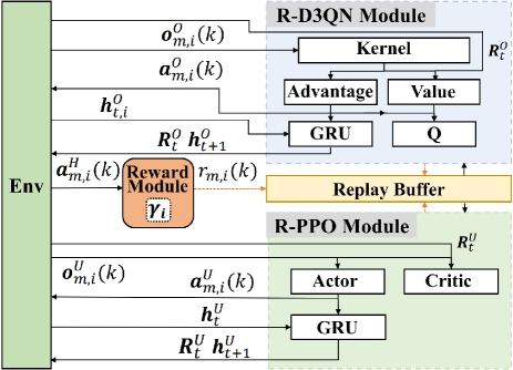
As shown in Fig. 6, for each mobile device, our algorithm contains R-D3QN and R-PPO networks for discrete and continuous action space as well as interactions between agents and history information.
F-A R-D3QN Module
D3QN is a modified version of deep Q-learning [71] equipped with double DQN technique with target Q to overcome overestimation [72] and dueling DQN technique which separately estimates value function and advantage function [73]. And our R-D3QN structure is inspired by DRQN [74] which allows networks to retain context and memory from history events and environment states. The key idea is to learn a mapping from states in state space to the Q-value of actions in action space . When the policy is learned and updated to the mobile device, it can selective offloading actions with the maximum Q-value to maximize the expected long-term reward. Apart from traditional deep Q-learning, it has a target Q-function network to compute the expected long-term reward of based on the optimal action chosen with the traditional Q-function network to solve the overestimation problem. What’s more, both the Q-function networks contain the advantage layer and value layer, which are used to estimate the value of the state and the relative advantage of the action. What’s more, we take advantage of a GRU module to provide history information of other agents’ decisions and environment states.
F-B R-PPO Module
R-PPO mainly includes two networks: policy network and value network. Policy network is responsible for producing actions based on networks. It outputs mean and standard deviation vectors for continuous action and probability distribution for discrete network. The value network computes the advantage values and estimates the expected return of the current state. Similar to R-D3QN network, it has an additional GRU module to memory the state-action pairs from history and other agents to enhance the information contained by the state based on which the value network estimates the state value.