Conditional Testing based on Localized Conformal -values
Abstract
In this paper, we address conditional testing problems through the conformal inference framework. We define the localized conformal -values by inverting prediction intervals and prove their theoretical properties. These defined -values are then applied to several conditional testing problems to illustrate their practicality. Firstly, we propose a conditional outlier detection procedure to test for outliers in the conditional distribution with finite-sample false discovery rate (FDR) control. We also introduce a novel conditional label screening problem with the goal of screening multivariate response variables and propose a screening procedure to control the family-wise error rate (FWER). Finally, we consider the two-sample conditional distribution test and define a weighted U-statistic through the aggregation of localized -values. Numerical simulations and real-data examples validate the superior performance of our proposed strategies.
Keywords: Conditional testing; Conformal inference; False discovery rate; Family-wise error rate; U-statistic.
1 Introduction
Nowadays, conformal inference has become an increasingly popular framework for quantifying uncertainty of machine learning models. Suppose we have i.i.d. training data and test data , where test responses are unobserved. The goal is to construct prediction intervals for with marginal coverage guarantee
| (1) |
By sample splitting or cross-fitting, conformal prediction methods (Vovk et al., 2005) can be coupled with any machine learning algorithm to construct distribution-free prediction intervals with finite-sample coverage guarantee. However, the marginal coverage (1) alone is not sufficient for an efficient prediction interval. A marginally valid prediction interval could have a miscoverage rate much higher than in some subgroups of the data. Therefore, the conditional coverage is also an important aspect:
| (2) |
Although appealing, achieving (2) in a finite-sample and distribution-free context is impossible (Vovk, 2013). Recent works have proposed many methods to construct prediction intervals with approximate or asymptotic conditional coverage guarantee by either modifying the calibration step (Lei and Wasserman, 2013; Guan, 2023) or using different score functions (Romano et al., 2019; Chernozhukov et al., 2021).
In addition to prediction intervals, the conformal inference framework is also valuable for other inference problems. With a similar calibration procedure, the conformal -value is defined to address various testing problems. This includes classical two-sample tests (Hu and Lei, 2023) and multiple testing problems such as outlier detection (Bates et al., 2023; Zhang et al., 2022) and data selection/sampling (Jin and Candès, 2023b; Wu et al., 2023). Therefore, as a parallel development, our paper moves beyond conditional prediction intervals and defines conformal -values tailored for conditional testing problems.
We define localized conformal -values by leveraging recent works Guan (2023) and Hore and Barber (2023) which constructed prediction intervals to adapt to the conditional distribution of the response. We present some fundamental properties of our defined -values and demonstrate why they can effectively resolve these problems. More importantly, we also consider several non-trivial applications of localized conformal -values, encompassing various testing problems with different error criteria (e.g., FDR, FWER or type I error). We show that the proposed testing rule can ensure valid corresponding error rate control. Here we provide a brief overview of those problems and defer rigorous formulations to later sections.
-
•
Conditional outlier detection: Outlyingness in data sets may come from various forms of heterogeneity. One of the important cases is that a few individuals in the test data do not share the same regression functions with majority (Peng et al., 2023). This amounts to detecting outliers in the functional relationship between the response and covariates that can be represented by the conditional distribution of . This is common in many spatial or temporal contexts where the scale or variance of the response variable varies with location or time (Catterson et al., 2010).
-
•
Two-sample conditional distribution test: The goal is to test for equality of conditional distributions of between two samples (Hu and Lei, 2023). This is also known as the problem of comparison of regression curves (Dette and Neumeyer, 2003). Some contemporary applications include assessing casuality by testing whether the conditional distribution of the response given the covariates remains the same between two samples (Bühlmann, 2020) and testing whether the pre-trained model can still perform well on a new test sample (Farahani et al., 2021).
-
•
Conditional label screening: Consider a scenario where the response is multivariate. Our goal is to determine whether each component of the response satisfies a pre-specified rule for an unlabeled data point. For example, in the LLM factuality problem (Mohri and Hashimoto, 2024; Cherian et al., 2024) we have a vector of claims output by a LLM. It is desirable to screen out false claims to ensure reliability. In this example, the conditional performance of the screening procedure is important, which needs to be addressed properly to avoid extreme or imbalanced results.
1.1 Our contributions
In this article, building on Hore and Barber (2023)’s randomly localized conformal prediction interval, we construct localized conformal -values, study their theoretical properties, and apply them to several conditional testing problems. Our contributions to the applications are as follows:
- •
-
•
We elaborate a novel conditional label screening problem with rigorous formulation. We use the localized conformal -value to construct a screening procedure with finite-sample marginal FWER control. We also present a conditional FWER inflation bound of our procedure to demonstrate its robustness against conditionality.
-
•
We propose a U-statistic for the two-sample conditional distribution testing problem by aggregating the localized conformal -values. The asymptotic normality of the test statistic under null and local alternatives is established.
We also validate our methods through simulations and real-data experiments. With commonly used prediction algorithms, our proposed methods exhibit superiority in terms of both validity and power compared to existing approaches.
1.2 Related works
Conformal inference was originally designed to construct prediction intervals and enjoy valid and distribution-free properties with the only assumption that the data are exchangeable. There have been several extensions to this framework. For example, Tibshirani et al. (2019) proposed weighted conformal prediction for covariate shift settings, and Romano et al. (2019) introduced conformalized quantile regression to account for heteroscedasticity. Other applications of the conformal inference framework include causal inference (Lei and Candès, 2021), selective inference (Bao et al., 2024), and survival analysis (Candès et al., 2023), among others.
Besides conformal inference, we also briefly review recent literature about our application problems.
-
•
Outlier detection. Classical outlier detection methods include multivariate outlier detection methods that use model assumptions to identify outliers (Riani et al., 2009; Cerioli, 2010), and machine learning algorithms (Liu et al., 2008; Erfani et al., 2016). Most existing works on conditional outlier detection fall into these two categories (Song et al., 2007; Catterson et al., 2010; Hong and Hauskrecht, 2015). Recent studies have used the conformal inference framework to test for outliers with advanced machine learning models (Bates et al., 2023; Marandon et al., 2024; Liang et al., 2024). Although these methods ensure finite-sample FDR control, they focus primarily on marginal cases and do not address outlier detection in conditional distributions.
-
•
Two-sample conditional distribution test. Most existing works focus on testing the equality of two conditional moments (Hall and Hart, 1990; Dette and Neumeyer, 2003), which is less stringent than testing for equality of distributions. A notable contribution is Hu and Lei (2023), which proposed a U-statistic based on the conformal inference framework by aggregating conformal -values. Chen and Lei (2024) improved this method by de-biasing the functions estimated using machine learning algorithms. Our porposed test statistic, a kernel-weighted U-statistic, is closely related to Hu and Lei (2023) by aggregating localized conformal -values instead.
-
•
Data selection and subsampling. Our introduced label screening problem is similar to label-based data selection (Jin and Candès, 2023a, b; Rava et al., 2021) and subsampling problems (Wu et al., 2023). These works consider a semi-supervised setting where the selection or sampling rule is based on the value of the response variable. The key difference in our problem is that we focus on screening within the multivariate response vector for each data point, rather than selecting different data points from the unlabeled dataset. Additionally, existing works do not account for the conditional properties of their methods, which is the main concern of our paper.
1.3 Organization and notations
The remainder of this paper is organized as follows. We briefly review conformal inference and then give the definitions and theoretical properties of the localized conformal -value in Section 2. In Section 3, we apply the proposed -values to several conditional testing problems. Simulation and real-data experiments results for all three applications are displayed in Section 4 and Section 5. Finally, we conclude the article in Section 6 with some remarks.
Notations. The is the indicator function and are the - and -norm. The denotes the set . The denotes the point mass at value . The notation denotes the -th quantile of distribution . The subscripts of and indicate distributions of random variables in the expectations and probabilities.
2 Localized conformal -values
In this section, we first revisit the definition of the split conformal prediction and its localized extensions by Guan (2023) and Hore and Barber (2023) in Section 2.1. Then we propose the localized conformal -values by inverting the localized prediction intervals in Section 2.2. At last we discuss basic properties of the defined -values in Section 2.3.
2.1 Recap: conformal prediction and localization
We consider data pair . Suppose we have and with each data point . In different problems, the responses of the second sample can be observed or unobserved.
In the classical split conformal prediction, is divided into the training and calibration sets with index sets . The training set is used to train a prediction function for the response and construct a non-conformity function which measures the similarity between the prediction and the true response. We then apply the score function to the calibration set to compute calibration scores and obtain the quantile threshold
| (3) |
The split conformal prediction interval is defined as If are exchangeable, the prediction interval is finite-sample valid in the sense that .
However, calibrating marginally with (3) does not account for the local information of the test point. Guan (2023) proposed the localized conformal prediction by calibrating with the quantile of a weighted empirical distribution
where for some kernel function characterizing the similarity between its two arguments. Here is the adjusted level to guarantee finite-sample coverage. Despite its efficiency, the LCP method needs to compute the adjusted level , which is complex and computationally inefficient. As an improvement, Hore and Barber (2023) proposed a randomization technique to circumvent level adjustment. Their method first samples from the distribution , takes the threshold as
and define the prediction interval as
| (4) |
where . If are exchangeable, we can compute the density ratio of and conditional on as
which exactly matches the weights in the empirical distribution. By the weighted exchangeability in Tibshirani et al. (2019), the randomly localized conformal prediction interval is finite-sample valid in the sense that
2.2 From prediction intervals to -values
Motivated by the capability of (randomly) localized conformal prediction to capture local information, we invert these prediction intervals to construct the localized conformal -value. Due to its simplicity, we follow Hore and Barber (2023) and take the randomization technique as in (4).
Let be a bi-variate kernel function with bandwidth
where is a kernel density function. Here can be taken as the Gaussian kernel, the box kernel or any other nonparametric kernel function as long as it is a symmetric density function. Define the localized conformal -value for as
| (5) |
where is an independent random variable and is randomly sampled from density . The non-conformity score may depend on both and or only on , contingent on the specific problem. The can be viewed as a localized counterpart of the conformal -value investigated by Bates et al. (2023) by using weighted empirical distributions. To simplify terminology, we will use CP and LCP to refer to the unweighted conformal -value and our localized conformal -value, respectively in the rest of the article. Since we do not discuss prediction intervals, this should not lead to confusion.
2.3 Basic properties
In this section we state some basic properties of the localized conformal -value. The first property is its finite-sample validity.
Theorem 1.
Under the condition , the localized conformal -value satisfies
Furthermore, if the score has a continuous distribution, then
This theorem is a direct corollary of the weighted exchangeability of given . By leveraging this property, the LCP can be used for multiple testing to guarantee finite-sample FDR or FWER control.
By the nature of the local-weighting scheme, the LCP can adapt to potential covariate shifts. The following theorem is an analog of the robustness result in Hore and Barber (2023).
Theorem 2.
Under the condition , denote the covariate density ratio as . The LCP satisfies
where the distribution has a density function .
This theorem gives a deviation bound of the distribution of LCP from uniform distribution under covariate shift. The excess term will be small with a small when the density ratio function satisfies some regularity conditions. For example, if is Lipchitz continuous, the excess term will vanish as . If we otherwise take as the normalized indicator of some fixed , the excess term will also vanish, indicating the LCP is approximately valid conditional on any fixed subset .
As an indirect power characterization, the next theorem studies the point-wise limit of the LCP function which is defined as
where and is sampled from . With a score function chosen properly based on the specific problem, a larger score value will indicate stronger evidence against the pre-specified null hypothesis. Our defined -value therefore reflects evidence against the null contained in a single data point. For the -value to be powerful, the value of should be small if is sampled under the alternative. Therefore, for a fixed score value under the alternative, we can regard a -value function to be asymptotically more powerful than another if its limit function takes smaller value at .
We need some regularity conditions which are commonly used in nonparametric estimations.
Assumption 1.
The following conditions hold for :
-
•
has a continuous distribution with bounded density;
-
•
The conditional distribution of the score satisfies
for some constant . That is, the conditional distribution function varies smoothly with .
-
•
The density function is continuous, and the conditional density function is continuous in .
Theorem 3.
Assume Assumption 1 holds and the split ratio for some constant , then the LCP function converges in probability
for any fixed , as .
By the weak law of large number, the unweighted CP function satisfies
where is the marginal distribution function of score . If we take such that , the LCP function converges to in probability. Comparing the power then amounts to comparing the value of and . For a score value under the alternative, our conditional testing problem can generally ensure a uniformly small value of since the signal lies in the deviation of the conditional distribution. In contrast, the value of could be quite large for pairs with a small conditional scale , even if these pairs are sampled under the alternative. Although not uniformly more powerful, the LCP can identify signals in these regions of with a small conditional scale , which tends to be missed by the CP. This property further motivates us to apply the LCP on conditional testing problems.
Remark 1.
The deviation bound in Theorem 3 has two terms corresponding to the bias and variance of -value functions. This is different from Theorem 2 in which we only need to eliminate bias and ensure validity. Fixing the sample size and taking , the LCP will degenerate to the independent uniform random variable , which remains valid but does not contain any information of the data. Otherwise if we take it will degenerate to the unweighted CP. Therefore, the bandwidth controls the trade-off between the conditional validity of the LCP and the effective sample size.
3 Applications on conditional testing
In this section, we apply the LCP on several conditional testing problems. We first provide a straightforward application on sample selection problem in Section 3.1. Then in Section 3.2 we study the conditional outlier detection problem and adopt the conditional calibration technique to achieve finite-sample FDR control. In Section 3.3 we introduce a novel conditional label screening problem and leverage the LCP to design a screening procedure with FWER control. Finally, we propose a two-sample U-statistic by aggregating the simplified LCP for the two-sample conditional distribution test in Section 3.4.
3.1 Warm-up: balanced data selection
Consider the sample selection problem which was investigated by Jin and Candès (2023b) and Wu et al. (2023). The test sample is unlabeled. The goal is to select test samples satisfying a pre-specified rule . Therefore, whether to select the th sample amounts to conducting the following hypothesis test:
In this case, the CP can be accordingly defined as
and if we select . Such methods directly controls the per selection error rate (PSER), say
Analogously, we can apply our proposed localized conformal -value instead to achieve certain improvement in terms of conditional performance. The LCP is defined as
where is a non-conformity score function depending on . We use to indicate selecting or not, where . As a corollary of Theorems 1-2, the following theorem provides the marginal and conditional properties of this simple selection rule.
Theorem 4.
Suppose and are exchangeable, the selection rule can ensure finite-sample marginal PSER control . Moreover, the conditional PSER inflation bound is given by
where is the conditional density of , has a density function and is the boundary set of .
The second result is obtained by taking the function in Theorem 2 and simplifying the deviation term. For general sets of regular form (e.g., balls or hypercubes), the excess term will be small with a small . This indicates that using the LCP for data selection can lead to a more balanced selection result since the PSER inflation for different sub-groups is bounded. For instance, by choosing an appropriate , we can expect that the burden of incorrect selection probability (PSER) will be more evenly distributed among different genders and races via our LCP. Similar issue is also considered by Rava et al. (2021) from the perspective of fairness.
3.2 Conditional outlier detection
In the conditional outlier detection problem, the available data consists of clean data and test data with potential outliers. Both samples are labeled with observed responses. The inliers in have the same conditional distribution with while the outliers may have different conditional distributions from each other. Detecting conditional outliers can be formulated as the following multiple testing problem:
| (6) |
where is an inlier if holds and outlier if holds. Our goal is to determine the detection set (or the rejection set equivalently) based on the observed data and . Denote as the index sets of inliers and outliers. The rejection set should contain as many indices in as possible while guaranteeing finite-sample false discovery rate (FDR) control
Bates et al. (2023) utilized the conformal -value to test for marginal outliers by applying the BH procedure on conformal -values computed on the test data. However, this is generally not effective when testing for conditional outliers. As discussed in the previous section, the classical CP targets on the joint distribution of rather than , and thus cannot identify all information in the conditional distribution of score variables. In light of the capability of the LCP to capture deviations in conditional distributions, we can take it as a refinement to detect conditional outliers.
As proved by Bates et al. (2023), the unweighted conformal -values based on the same calibration set is PRDS, under which the BH procedure can still guarantee finite-sample FDR control. This property, however, does not hold for the weighted conformal -values. In order to achieve the finite-sample property, we adopt the conditional calibration technique (Fithian and Lei, 2022) to prune the rejection set output by the BH procedure.
To perform multiple testing with the LCP, we first train the non-conformity score function on and then compute scores and on and , respectively. After sampling for each , the LCP’s are computed as in Eq. (5). Define the auxiliary -values as
| (7) |
for . Let be the rejection set of the BH procedure applied on and be the initial rejection set. We determine the final rejection set by generating independent and pruning into
| (8) |
where .
The outlier detection procedure is summarized in Algorithm 1.
The following theorems shows that our detection procedure can guarantee finite-sample FDR control if the distribution of the covariates does not change.
Theorem 5 (Finite-sample FDR control).
Under the condition that , the final output given by Algorithm 1 ensures .
Remark 2.
Testing for conditional outliers may not be restricted to the regression setting. Consider the case where only the covariate is available. By splitting the covariate vector into , one can compute weights with respect to and test for outliers regarding the conditional distribution . This approach is applicable in various spatial or temporal settings where can be taken as the location or time variable.
3.3 Conditional label screening
In the conditional label screening problem, the response variable is multivariate with for some random variable . The first sample is the labeled data while the second sample is unlabeled. The response vectors are denoted as for . Our goal is to determine whether each component of the unobserved response satisfies a pre-specified rule for each . For each entry , we define the screening rule as with pre-chosen sets . This can be formulated as a multiple testing problem for each test sample
| (9) |
For example, Mohri and Hashimoto (2024); Cherian et al. (2024) considered using conformal prediction techniques to improve the output factuality of large language models (LLM). Specifically, they transform the output of the LLM into a set of claims and aim to construct a filtered claim set that contains no false claims with high probability. Such application can be framed into our conditional label screening problem stated above. The covariate includes the input prompt , the output of the LLM model and a claim vector of length summarized by another language model. The response vector is a 0-1 vector with or indicating whether the corresponding claim is correct or not. Here we can take for every to screen out false claims.
To ensure reliability of the screening procedure, we seek to control the probability of failing to screen out any component of that does not meet the rule. Let or indicate whether is retained after screening. This can be rigorously formulated as
| (10) |
say, controlling the FWER for (9). However, the marginal FWER might not be sufficient in real problems. We can use the localization technique to improved conditional validity while still guaranteeing marginal FWER control.
Since the test data is unlabeled in the current problem, the non-conformity score function should depend only on the covariate . We can use the training data to estimate the probability . This can be achieved by training classification models for each component of if the length is a fixed constant or fitting a joint classification model that outputs a probability vector. In both scenarios, we can define the score vector
where each approximates . By this definition, we should reject if is large, and controlling the FWER amounts to examining the distribution of . This motivates us to define the localized -value
| (11) |
where . We can show that the ’s satisfy the group super-uniform property, i.e.,
and thus we can screen out components of with , We summarize our label screening procedure in Algorithm 2.
We have the following result.
Theorem 6.
Suppose are exchangeable, then the label screening procedure given by Algorithm 2 ensures finite-sample FWER control
Regarding the conditional property, we can also establish the finite-sample conditional FWER deviation bound for our procedure.
Theorem 7.
Suppose the assumptions in Theorem 6 hold. For any fixed set with , the conditional FWER has the following bound
where is the boundary of set .
In this theorem, the inflation bound is similar to that in the second result of Theorem 4. By a similar rationale, this demonstrate the advantage of our method to mitigate conditional error rate inflation.
3.4 Two-sample conditional distribution test
In the two-sample conditional testing problem, the second sample is labeled and i.i.d. following a potentially different distribution from the first sample . The conditional distribution test can be formulated as
| (12) |
Hu and Lei (2023) proposed a two-sample conditional distribution test based on the conformal inference framework. To be specific, they first split both samples as and with . For notation convenience, we perform an equal-sized sample splitting with and let in this section. Thereafter, the score function and density ratio estimator
are trained on by fitting classification models to distinguish and . After computing scores and , the weighted conformal -values are obtained as
The test statistic is constructed by averaging these -values
where and is the variance estimator. Under the null hypothesis, they proved that is asymptotically normally distributed and the rejection region is given by .
We extend the above strategy by aggregating the localized conformal -values computed on the second sample. Since -values are no longer necessary to be finite-sample valid in this case, here we use a simplified variant of the localized conformal -value without randomization
| (13) |
and our proposed test statistic is defined as
| (14) |
where and is the variance estimator. This test statistic is constructed by averaging unnormalized LCP’s in Eq. (13) and performing standardization. From a different perspective, it is also related to the classical U-statistic for model checking problems (Zheng, 1996; Gao and Gijbels, 2008) in which the ’s are replaced by the residuals. Inherited from the nice property of conformal techniques, our method enjoys model-agnostic features and allows us to employ state-of-the-art algorithms to construct efficient score function that is able to better measure the discrepancy between two conditional distributions.
We need the following technical assumptions to establish the asymptotic normality of . We also make the same regularity assumptions to those in Hu and Lei (2023) without further declaration in theorems, which guarantee identifiability of the problem.
Assumption 2.
Let be the true conditional density ratio. Denote the oracle statistics as and . Suppose that
-
•
has a continuous distribution;
-
•
.
Recall that we use classification to construct the score function to approximate the true conditional density ratio in this problem. This assumption requires the approximation error is sufficiently small after local-weighting. A similar assumption has been made in Hu and Lei (2023) with replaced by . These two assumptions are introduced both to ensure a vanishing asymptotic bias and achieve asymptotic normality in the presence of covariate shift.
Theorem 8 (Asymptotic normality).
Note that the convergence of the score function is only needed under covariate shift settings. Given the asymptotic normality property, we can construct our testing procedure as summarized in Algorithm 3.
Theorem 9 (Behavior under local alternatives).
This theorem is similar to Proposition 1 in Hu and Lei (2023). The main difference lies in the form of “signal strength” , which is in their article. In comparison, the difference term in is based on the same covariate value and therefore better captures the deviation in conditional distribution. This reflects the superiority of our proposed test statistic in the two-sample conditional testing problem.
4 Simulation experiments
In this section, we provide extensive synthetic experiment results to show the validity and efficiency of our proposed methods for three main applications in Sections 4.1-4.3, respectively.
4.1 Results for conditional outlier detection
For the conditional outlier detection problem, we consider two scenarios:
-
•
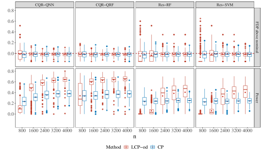
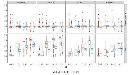
Scenario A1 (with label ): A heterogeneous linear regression model. The covariate vector consists of with and an additional time feature . The model is
with and independently. The coefficient vector is . The test data contains outliers following the model
where and .
-
•
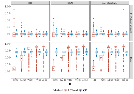
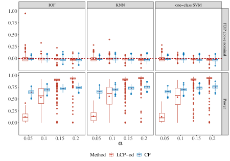
Scenario B1 (without label ): Another example which does not include the label . To fit our problem, we consider a spatial setting with where is the spatial variable and contains the remaining features. We consider with and with :
where independently. The test data contains outliers with the same distribution for and a different conditional distribution
Benchmarks. We abbreviate our method as LCP-od (outlier detection) and compare it with a benchmark method abbreviated as CP. The CP method is implemented by computing the unweighted conformal -values as defined in Bates et al. (2023) and then applying the BH procedure. For the LCP-od and CP methods, we use two score functions and apply various regression or classification algorithms, which are detailed in the implementation part.
Implementation details. Since our goal is to test for outliers conditional on or in Scenarios A1 and B1, we only use these variables when computing the weights. For both scenarios, the kernel function of the LCP-od method is taken as the Gaussian kernel with bandwidth for in Scenarios A1 and B1. This corresponds to the optimal convergence rate for . For Scenario A1, we consider two kinds of score functions: the CQR score and the absolute residual of different regression algorithms. Similar to Romano et al. (2019), for the CQR score, we consider using quantile neural networks (CQR-QNN) and quantile random forests (CQR-QRF). For the absolute residual score, we take two regression algorithms: random forest (Res-RF), and support vector machine (Res-SVM). For Scenario B1, we use one-class classifiers for both the LCP-od and CP methods. We take three kinds of one-class classification algorithms: the isolation forest (IOF), -Nearest-Neighbor (-NN) with and one-class support vector machine (one-class SVM).
Results. For each scenario, we consider either fixing and varying or fixing the sample size and varying . The results for Scenario A1 are shown in Figure 1-2, and the results for Scenario B1 are shown in Figure 3-4. In both scenarios, the LCP-od method accurately controls the FDR around the nominal level, which validates its finite-sample FDR control property. In terms of power, the LCP-od method demonstrates higher power than the CP benchmark in Scenario A1 with both two score functions when the sample size and the nominal level are relatively large. Compared with the absolute residual score, the CQR score leads to relatively higher power due to its adaptivity to the conditional distribution . However, the power gain is still significant after applying the LCP-od method, illustrating the advantage of local weighting.
In Scenario B1, the power of the LCP-od method grows significantly with the sample size and the nominal level , while the power of the CP method only rises slightly. As discussed in the main text, the unweighted CP cannot identify those outliers with small conditional variance of the score. This explains why the power of the CP method remains “stuck” around the same value. In contrast, the power of the LCP-od method approaches 1 as the sample size increases, demonstrating the full identifiability of the LCP-od method in testing for conditional outliers.
4.2 Results for conditional label screening
For the conditional label screening problem, we consider a nonlinear regression model:
-
•
Scenario A2 (nonlinear regression): We take a constant and the response with , , and . The screening target is where is the 70% quantile of for , respectively.
Implementation details. We fix the sample sizes and vary . We apply three different algorithms to train a probability prediction function for each component of : linear logistic regression (LL), neural network (NN) and random forest (RF).
Benchmarks. We compare our conditional label screening method via the LCP (abbreviated as LCP-ls) as summarised in Algorithm 2 with the thresholding procedure without weighting (abbreviated as THR). The THR method is performed by only replacing the LCP by the classical unweighted CP.
Results. We calculate the empirical marginal FWER and four kinds of conditional FWER’s (conditional on for four different sets ). The evaluation measures are defined as follows:
-
•
(Marginal FWER):
-
•
(Conditional FWER): for and , where , , , and .
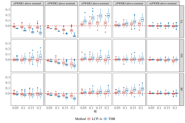
The results for Scenario A2 are reported in Figure 5. As theoretically ensured, both methods control the marginal FWER at nominal levels. However, the LCP-ls is much more robust against conditionality and exhibit a much smaller conditional FWER inflation than the THR method on subsets and . Accordingly, while the FWER conditional on of both the THR and LCP-ls methods approach 0 as the nominal level increases, the conditional error rate of the LCP-ls method remains much closer to the nominal level. This also suggests that the LCP-ls method offers a more balanced screening result.
4.3 Results for two-sample conditional distribution test
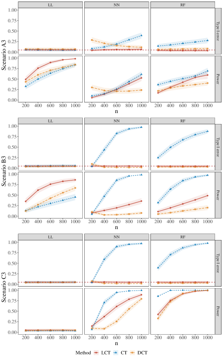
We consider three different scenarios for the problem of two-sample conditional distribution test, which are analogous to those in Hu and Lei (2023):
Scenario A3: Let and , where with and independently. We set under the null and under the alternative.
Scenario B3: Let and , where with , and independently. We set under the null and under the alternative.
Scenario C3: Let and , where is an additive function of B-splines, and with , and we set under the null and , under the alternative.
Implementation details. Under each scenario, we fix and consider different sample sizes with equal splitting. The coefficient in model A and B are taken as . For our localized conformal test (LCT) method, we take the Gaussian kernel function and choose the same bandwidth . For all three scenarios, we use three different probabilistic classification models to estimate density ratios: linear logistic (LL), random forest (RF) and neural network (NN). The type I error (size) under the null and the power under the alternative are calculated for each scenario across 500 replications with nominal type I error level .
Benchmarks. We compare our localized conformal test (LCT) as summarised in Algorithm 3 with the following two tests:
- •
-
•
DCT: Chen and Lei (2024)’s de-biased conformal test, where they formulate the covariate shift problem within the nonparametric framework and utilize the doubly-robust technique to correct the bias of the test statistic.
Results. The results for all three scenarios are summarised in Figure 6. Regarding type I error, the CT method is only valid when the training model is correctly specified and exhibits a severely inflated type I error rate under mis-specified models. The DCT method is more robust than the CT method and controls the type I error rate under the nominal level for most scenarios and training models. This corresponds to its doubly-robust property, which relaxes the requirement on accuracy of the estimated density ratios. In contrast, the LCT method controls the type I error rate accurately around the nominal level for any combination of scenario and training model. This shows the robustness and wide applicability of our proposed test statistic.
In terms of power, the CT method is not valid with misspecified training models, so we only discuss the DCT and LCT methods. In Scenarios A3 and B3, the LCT method exhibits higher power than the DCT method especially when the sample size is large. In Scenario C3, the LCT method is more powerful than the DCT method using the NN algorithm and the two methods perform similarly when using the LL or RF algorithm. In general, the power improvement is more significant when the classification algorithm can distinguish the two populations better. Except for the numerical performance, the DCT method involves not only data splitting but also a cross-fitting step. The LCT test does not require the latter and is therefore much easier to implement and computationally more efficient.
5 Real data examples
5.1 Conditional outlier detection on spatial data
Dataset. We use the House Sales in the King County, USA dataset (Kaggle, 2016) to demonstrate the performance of our method in a spatial scenario with label . The dataset contains observations with 21 attributes including two spatial features: longitude () and latitude (). The response is the price of houses.
Implementation details. We randomly sample three parts of the data from the whole dataset: training data, calibration data and test data. Since the original dataset contains no conditional outliers, we create synthetic outliers and apply different methods for detection. We randomly sample 10% of the testing data to be outliers. For the outliers, we add a random noise to the original response . We consider two kinds of synthetic outliers.
-
•
Conditional quantile-based outlier:
where is the 90% conditional quantile of given and .
-
•
Conditional variance-based outlier:
where is the conditional variance of given and .
All results are based on 500 replications.
Results. We compare the LCP-od and the CP methods with the CQR score constructed by two different algorithms: quantile random forest (QRF) and quantile neural network (QNN). The empirical FDR and power for conditional outlier detection are reported in Table 1-2. The result is similar to the simulation part, where all methods control the FDR below the nominal. While the advantage is not as significant as before, the LCP-od method still enjoys the highest power in all cases.
| Method | LCP-od | CP | |||
|---|---|---|---|---|---|
| Score | CQR-QNN | CQR-QRF | CQR-QNN | CQR-QRF | |
| 0.15 | FDR | 0.139 (0.087) | 0.131 (0.030) | 0.128 (0.047) | 0.145 (0.036) |
| Power | 0.657 (0.096) | 0.871 (0.048) | 0.593 (0.037) | 0.858 (0.070) | |
| 0.2 | FDR | 0.177 (0.033) | 0.175 (0.030) | 0.174 (0.049) | 0.175 (0.037) |
| Power | 0.882 (0.131) | 0.913 (0.021) | 0.824 (0.078) | 0.907 (0.022) | |
| Method | LCP-od | CP | |||
|---|---|---|---|---|---|
| Score | CQR-QNN | CQR-QRF | CQR-QNN | CQR-QRF | |
| 0.15 | FDR | 0.141 (0.051) | 0.127 (0.029) | 0.142 (0.043) | 0.128 (0.035) |
| Power | 0.520 (0.168) | 0.628 (0.092) | 0.480 (0.085) | 0.581 (0.119) | |
| 0.2 | FDR | 0.181 (0.036) | 0.176 (0.038) | 0.196 (0.034) | 0.186 (0.030) |
| Power | 0.630 (0.084) | 0.722 (0.056) | 0.597 (0.099) | 0.692 (0.106) | |
5.2 Conditional label screening on health data
Dataset. We use the health indicators dataset from Kaggle (Kaggle, 2021) to illustrate the performance of our conditional label screening method. The dataset comprises samples and 22 variables, including demographic attributes (e.g., sex, age, BMI), lifestyle-related features, as well as several binary health indicators. These indicators capture whether an individual has conditions such as diabetes, coronary heart disease, or has experienced a myocardial infarction, among others. Accordingly, we define the response variable Y as these disease-related binary labels, with the goal of predicting the risk of these conditions in test data. More specifically, the response vector is set as follows:
-
•
: Indicates whether an individual has diabetes.
-
•
: Indicates whether an individual has coronary heart disease or myocardial infarction.
-
•
: Indicates whether an individual has experienced a stroke.
Consequently, the label screening targets are for .
Implementation details. We fix the size of the labeled data at and the test data at , randomly sampling them from the original dataset without replacement in each replication. We fix the nominal level at , and apply two different algorithms to compute the score vectors: linear logistic regression (LL) and random forest (RF). We calculate the empirical marginal FWER and conditional FWER (conditional on for a specific set ) across 500 replications for the screening procedure via LCP-ls and the simple thresholding rule, respectively. The evaluation measures are defined as follows:
-
•
(Marginal FWER):
-
•
(Conditional FWER): for , where .
Results. We show the average of measures for all test samples. The results are reported in Table 3. We observe that both benchmarks can ensure valid marginal FWER control, while only the label screening procedure via the LCP-ls is capable of controlling both conditional and marginal FWER simultaneously.
| Method | ||||
|---|---|---|---|---|
| LCP-ls | 0.0329 (0.018) | 0.0372 (0.018) | 0.0487 (0.009) | 0.0507 (0.009) |
| THR | 0.0740 (0.028) | 0.0887 (0.029) | 0.0500 (0.011) | 0.0538 (0.012) |
5.3 Two-sample conditional distribution test on the airfoil data
Dataset. Refer to previous related works (Hu and Lei, 2023; Chen and Lei, 2024), we consider using the airfoil dataset (Brooks et al., 2014) from the UCI Machine Learning Repository to demonstrate the effectiveness of our proposed LCT on real data. This dataset investigates the sound pressure of various airfoils with observations of the response : the scaled sound pressure and the covariates with dimensions: log frequency, angle of attack, chord length, free-stream velocity, and suction side log displacement thickness.
Implementation details. We use part of the rules in Hu and Lei (2023) to split the observations into two samples as follows:
-
(i)
Random partition. Randomly partition the dataset into two groups with sizes and .
-
(ii)
Exponential tilting. First randomly partition the data into . Then construct by sampling 25% of the points from with replacement, with probabilities proportional to , where .
-
(iii)
Partition along the response. Split the data according to the value of response, where the first group contains the samples with smaller response values.
In the first two partitions, the two samples satisfy the null hypothesis. The first partition has samples from the same distribution, while the second shows a non-trivial covariate shift. In the last partition, the covariate shift assumption is not satisfied and the alternative hypothesis holds. For all three cases, we use the linear logistic (LL) and neural network (NN) to estimate the density ratios. All results are based on 500 replications.
Results. Similar to Hu and Lei (2023), we use out-of-sample marginal classification error as a proxy of the accuracy of marginal density ratio estimation for all cases. The percentage of rejections for cases (i-ii) are summarised in Table 4. The rejection proportions of both the LCT and DCT methods are close to the nominal level when using LL or NN algorithms, while the CT test fails to control the type I error when using the NN algorithm due to its low accuracy. For case (iii), we only have a single deterministic generation of the training and test data for each replication. We therefore report the median -values for case (iii) in Table 5. While all three tests correctly reject the null, the LCT test gives the smallest -value and is therefore the most powerful among all three tests.
| Cases | Method | ||||
|---|---|---|---|---|---|
| Case (i) | LCT | 0.054 (0.0325) | 0.053 (0.0374) | 0.429 | 0.608 |
| CT | 0.058 (0.0289) | 0.441 (0.0610) | |||
| DCT | 0.053 (0.0299) | 0.066 (0.0268) | |||
| Case (ii) | LCT | 0.067 (0.0323) | 0.066 (0.0390) | 0.213 | 0.367 |
| CT | 0.056 (0.0320) | 0.135 (0.0405) | |||
| DCT | 0.056 (0.0327) | 0.035 (0.0250) |
| Cases | Method | ||||
|---|---|---|---|---|---|
| Case (iii) | LCT | 0.000 | 0.000 | 0.279 | 0.429 |
| CT | 0.000 | 0.022 | |||
| DCT | 0.000 | 0.018 |
6 Concluding remarks
We conclude the paper with two remarks. Firstly, the localized conformal prediction is efficient in capturing local or conditional information, but this comes at the cost of a much smaller effective sample size. In our simulation experiments, the power of localized methods grows significantly as the sample size increases in many scenarios. However, when the sample size is small, our proposed methods often exhibit lower power compared to other methods. Therefore, it would be beneficial to increase the effective sample size by utilizing additional data or modifying the definition of the LCP.
Secondly, we define the LCP with a random sampling step for each test point to achieve finite-sample validity. However, the random sampling step introduces external randomness, which degrades the stability of the related methods. Additionally, the LCP is defined by computing the similarity between covariates of the calibration data and the sampled covariate instead of the test point itself. Although these two issues are equivalent asymptotically, they generally differ in finite-samples. This makes the LCP not effective enough in characterizing local information. A potential solution is to use a different definition for the localized conformal -value to ensure finite-sample validity without randomization, which warrants further consideration.
References
- Bao et al. (2024) Bao, Y., Huo, Y., Ren, H., and Zou, C. (2024), “Selective conformal inference with false coverage-statement rate control,” Biometrika, asae010.
- Bates et al. (2023) Bates, S., Candès, E., Lei, L., Romano, Y., and Sesia, M. (2023), “Testing for outliers with conformal p-values,” The Annals of Statistics, 51, 149–178.
- Benjamini and Hochberg (1995) Benjamini, Y. and Hochberg, Y. (1995), “Controlling the false discovery rate: a practical and powerful approach to multiple testing,” Journal of the Royal Statistical Society: Series B (Statistical Methodology), 57, 289–300.
- Brooks et al. (2014) Brooks, T., Pope, D., and Marcolini, M. (2014), “Airfoil Self-Noise,” UCI Machine Learning Repository https://archive.ics.uci.edu/dataset/291/airfoil+self+noise.
- Bühlmann (2020) Bühlmann, P. (2020), “Invariance, Causality and Robustness,” Statistical Science, 35, 404–426.
- Candès et al. (2023) Candès, E., Lei, L., and Ren, Z. (2023), “Conformalized Survival Analysis,” Journal of the Royal Statistical Society: Series B, 85, 24–45.
- Catterson et al. (2010) Catterson, V. M., McArthur, S. D. J., and Moss, G. (2010), “Online Conditional Anomaly Detection in Multivariate Data for Transformer Monitoring,” IEEE Transactions on Power Delivery, 25, 2556–2564.
- Cerioli (2010) Cerioli, A. (2010), “Multivariate Outlier Detection with High-Breakdown Estimators,” Journal of the American Statistical Association, 105, 147–156.
- Chen and Lei (2024) Chen, Y. and Lei, J. (2024), “De-Biased Two-Sample U-Statistics With Application To Conditional Distribution Testing,” arXiv preprint arXiv:2402.00164.
- Cherian et al. (2024) Cherian, J. J., Gibbs, I., and Candès, E. J. (2024), “Large language model validity via enhanced conformal prediction methods,” arXiv preprint arXiv:2406.09714.
- Chernozhukov et al. (2021) Chernozhukov, V., Wüthrich, K., and Zhu, Y. (2021), “Distributional conformal prediction,” Proceedings of the National Academy of Sciences, 118, e2107794118.
- Dette and Neumeyer (2003) Dette, H. and Neumeyer, N. (2003), “Nonparametric comparison of regression curves: an empirical process approach,” The Annals of Statistics, 31, 880–920.
- Erfani et al. (2016) Erfani, S. M., Rajasegarar, S., Karunasekera, S., and Leckie, C. (2016), “High-dimensional and large-scale anomaly detection using a linear one-class SVM with deep learning,” Pattern Recognition, 58, 121–134.
- Farahani et al. (2021) Farahani, A., Voghoei, S., Rasheed, K., and Arabnia, H. R. (2021), “A Brief Review of Domain Adaptation,” in Advances in Data Science and Information Engineering, pp. 877–894.
- Fithian and Lei (2022) Fithian, W. and Lei, L. (2022), “Conditional calibration for false discovery rate control under dependence,” The Annals of Statistics, 50, 3091 – 3118.
- Gao and Gijbels (2008) Gao, J. and Gijbels, I. (2008), “Bandwidth Selection in Nonparametric Kernel Testing,” Journal of the American Statistical Association, 103, 1584–1594.
- Guan (2023) Guan, L. (2023), “Localized conformal prediction: A generalized inference framework for conformal prediction,” Biometrika, 110, 33–50.
- Hall and Hart (1990) Hall, P. and Hart, J. D. (1990), “Bootstrap Test for Difference Between Means in Nonparametric Regression,” Journal of the American Statistical Association, 85, 1039–1049.
- Hong and Hauskrecht (2015) Hong, C. and Hauskrecht, M. (2015), “MCODE: Multivariate Conditional Outlier Detection,” arXiv preprint arXiv:1505.04097.
- Hore and Barber (2023) Hore, R. and Barber, R. F. (2023), “Conformal prediction with local weights: randomization enables local guarantees,” arXiv preprint arXiv:2310.07850.
- Hu and Lei (2023) Hu, X. and Lei, J. (2023), “A Two-Sample Conditional Distribution Test Using Conformal Prediction and Weighted Rank Sum,” Journal of the American Statistical Association, 0, 1–19.
- Jin and Candès (2023a) Jin, Y. and Candès, E. J. (2023a), “Model-free selective inference under covariate shift via weighted conformal p-values,” arXiv preprint arXiv:2307.09291.
- Jin and Candès (2023b) — (2023b), “Selection by Prediction with Conformal p-values,” Journal of Machine Learning Research, 24, 1–41.
- Kaggle (2016) Kaggle (2016), “House Sales in King County, USA,” https://www.kaggle.com/datasets/harlfoxem/housesalesprediction.
- Kaggle (2021) — (2021), “Diabetes Health Indicators Dataset,” https://www.kaggle.com/datasets/alexteboul/diabetes-health-indicators-dataset.
- Lei and Wasserman (2013) Lei, J. and Wasserman, L. (2013), “Distribution-free Prediction Bands for Non-parametric Regression,” Journal of the Royal Statistical Society Series B: Statistical Methodology, 76, 71–96.
- Lei and Candès (2021) Lei, L. and Candès, E. J. (2021), “Conformal inference of counterfactuals and individual treatment effects,” Journal of the Royal Statistical Society Series B: Statistical Methodology, 83, 911–938.
- Liang et al. (2024) Liang, Z., Sesia, M., and Sun, W. (2024), “Integrative conformal p-values for out-of-distribution testing with labelled outliers,” Journal of the Royal Statistical Society Series B: Statistical Methodology, qkad138.
- Liu et al. (2008) Liu, F. T., Ting, K. M., and Zhou, Z.-H. (2008), “Isolation Forest,” in Proceedings of the 2008 Eighth IEEE International Conference on Data Mining, IEEE Computer Society, pp. 413–422.
- Marandon et al. (2024) Marandon, A., Lei, L., Mary, D., and Roquain, E. (2024), “Adaptive novelty detection with false discovery rate guarantee,” The Annals of Statistics, 52, 157 – 183.
- Mohri and Hashimoto (2024) Mohri, C. and Hashimoto, T. (2024), “Language Models with Conformal Factuality Guarantees,” arXiv preprint arXiv:2402.10978.
- Peng et al. (2023) Peng, L., Wang, G., and Zou, C. (2023), “MEASURING, TESTING, AND IDENTIFYING HETEROGENEITY OF LARGE PARALLEL DATASETS,” Statistica Sinica, 33, 1–22.
- Powell et al. (1989) Powell, J. L., Stock, J. H., and Stoker, T. M. (1989), “Semiparametric estimation of index coefficients,” Econometrica, 57, 1403–1430.
- Rava et al. (2021) Rava, B., Sun, W., James, G. M., and Tong, X. (2021), “A burden shared is a burden halved: A fairness-adjusted approach to classification,” arXiv preprint arXiv:2110.05720.
- Riani et al. (2009) Riani, M., Atkinson, A. C., and Cerioli, A. (2009), “Finding an Unknown Number of Multivariate Outliers,” Journal of the Royal Statistical Society: Series B (Statistical Methodology), 71, 447–466.
- Romano et al. (2019) Romano, Y., Patterson, E., and Candes, E. (2019), “Conformalized quantile regression,” Advances in Neural Information Processing Systems, 32.
- Song et al. (2007) Song, X., Wu, M., Jermaine, C., and Ranka, S. (2007), “Conditional Anomaly Detection,” IEEE Transactions on Knowledge and Data Engineering, 19, 631–645.
- Tibshirani et al. (2019) Tibshirani, R. J., Foygel Barber, R., Candes, E., and Ramdas, A. (2019), “Conformal Prediction Under Covariate Shift,” in Advances in Neural Information Processing Systems, vol. 32.
- Vovk (2013) Vovk, V. (2013), “Conditional validity of inductive conformal predictors,” Mach. Learn., 92, 349–376.
- Vovk et al. (2005) Vovk, V., Gammerman, A., and Shafer, G. (2005), Algorithmic learning in a random world, New York: Springer.
- Wu et al. (2023) Wu, X., Huo, Y., Ren, H., and Zou, C. (2023), “Optimal Subsampling via Predictive Inference,” Journal of the American Statistical Association, 0, 1–29.
- Zhang et al. (2022) Zhang, Y., Jiang, H., Ren, H., Zou, C., and Dou, D. (2022), “AutoMS: Automatic Model Selection for Novelty Detection with Error Rate Control,” in Advances in Neural Information Processing Systems, vol. 35, pp. 19917–19929.
- Zheng (1996) Zheng, J. X. (1996), “A consistent test of functional form via nonparametric estimation techniques,” Journal of Econometrics, 75, 263–289.
Appendix
Appendix A Technical details
A.1 Proof of Theorem 2
Proof. Denote as the marginal distribution of if we fist sample from or and then sample from . The distributions of the calibration and test points are and where and denote the corresponding conditional distributions of calibration and test data points.
Notice that the super-uniform property still holds if the conditional distribution . Therefore, the super-uniform bound holds for an independent tuple . That is
The probability for is then upper bounded by
For a fixed we have
Taking expectation with respect to we have
where has a density function .
By integration
Combining the results above we conclude
A.2 Proof of Theorem 3
Proof.
Remember the definition of the RBF and box kernel
where are normalizing constants.
The LCP function is
| (15) |
For the difference we have
For the denominator , first notice for the RBF kernel
Define , for constants we have
and
for sufficiently large , where only depends on . Taking we have
Therefore with probability tending to 1 we have for some fixed constant . Then
| (16) | ||||
For the first term
By integration
As all integrations in the final expressions exist, we have
Together with inequality (16) we complete the proof.
A.3 Proof of Theorem 4
Proof. By the construction of the refined LCP’s, they are valid conditional on the event in finite sample
and marginal PSER control result is proved. For the conditional PSER inflation bound, the proof is exactly the same to Theorem 7 with the only difference that the distribution of is replaced by the conditional distribution of given the event . We therefore delay the computation of the deviation term to the proof of Theorem 7.
A.4 Proof of Theorem 5
Proof.
Denote the index set of inliers in as , We firstly need a lemma commonly used in literature relating the conditional calibration technique.
Lemma A.1.
The pruned rejection set satisfies
Denote and as tuples and the index set of calibration data where . Let be the unordered value set of . Let be the set of all sampled covariates. Note that the unordered value set are fully determined by , and . Moreover, the -value is fully determined by , and . As is independent of conditional on , we know is independent of conditional on and . By the fact that is fully determined by , we further have
By the independency we have
where
By the weighted exchangeability, . Taking the expectation we have
which completes the proof.
A.5 Proof of Theorem 6
Define the uncomputable oracle -value as
By Theorem 1, if are exchangeable, this oracle -value will be super-uniform
Note that . This indicates
By direct tranformation we have
which completes the proof.
A.6 Proof of Theorem 7
Proof. By our screening procedure, the conditional FWER can be transformed as
Since we assume exchangeability, this is equivalent to the covariate shift setting with . Therefore, we only need to compute the excess term in Theorem 2 with this specific . By transformation
Following the same proof to Theorem 2 we conclude
A.7 Proof of Theorem 8
Proof. Remember that we assume in the main text. We first introduce a lemma about our defined U-statistic.
Lemma A.2.
For some kernel function depending on , define the two-sample U-statistic and its projection as
and
Then if , and satisfy
This theorem is an extension of Lemma 3.1 in Powell et al. (1989) which constructs a similar result for one sample U-statistics of degree 2. The proof follows exactly the same and is therefore omitted.
Denote the unnormalized version of and its projection as and . In our defined statistic . We first check the condition in Lemma A.2. By integration and
Together with the assumption we have .
Define the centralized projection statistics as and
The projection can be decomposed as
By Assumption 1 and we know . Similar results also hold for and .
Note that under the null hypothesis . So we have
If Assumption 2 holds then
If then under the null hypothesis we have and therefore by symmetric.
Now the statistic can be decomposed as
As and are independent random variables not depending on , we have
| (17) |
where
Hereafter we only need to prove the consistency of the variance estimator. Denote , the non-asymptotic variance can be decomposed as
By similar integration computation, the cross-term expectation converges to and in probability. Removing the vanishing term we have and .
The variance estimator takes the form
It is easy to see that consists of term-wise approximations of the expectations in . By further computing the second moments of the estimators and Markov’s inequality we have . Together with (17) we conclude
A.8 Proof of Theorem 9
Proof. By the same proof with Theorem 5 we know
| (18) |
By Assumption 2 we have . Combining with the consistency of we know and
The rest is to compute the bias term . By integration
And by transformation
The bias term is then simplified as
Combining all the results above we conclude
Appendix B Additional details
B.1 A flow chart of our work
![[Uncaptioned image]](/html/2409.16829/assets/x7.png)