Gripenberg-like algorithm for the lower spectral radius

Abstract.

This article presents an extended algorithm for computing the lower spectral radius of finite, non-negative matrix sets. Given a set of matrices $\mathcal{F}=\{A_{1},\ldots,A_{m}\}$, the lower spectral radius represents the minimal growth rate of sequences in the product semigroup generated by $\mathcal{F}$. This quantity is crucial for characterizing optimal stable trajectories in discrete dynamical systems of the form $x_{k+1}=A_{i_{k}}x_{k}$, where $A_{i_{k}}\in\mathcal{F}$ for all $k\geq 0$. For the well-known joint spectral radius (which represents the highest growth rate), a famous algorithm providing suitable lower and upper bounds and able to approximate the joint spectral radius with arbitrary accuracy was proposed by Gripenberg in 1996. For the lower spectral radius, where a lower bound is not directly available (contrarily to the joint spectral radius), this computation appears more challenging.

Our work extends Gripenberg’s approach to the lower spectral radius computation for non-negative matrix families. The proposed algorithm employs a time-varying antinorm and demonstrates rapid convergence. Its success is related to the property that the lower spectral radius can be obtained as a Gelfand limit, which was recently proved in Guglielmi and Zennaro (2020). Additionally, we propose an improvement to the classical Gripenberg algorithm for approximating the joint spectral radius of arbitrary matrix sets.

1. Introduction

The most important joint spectral characteristics of a set of linear operators are the joint spectral radius and the lower spectral radius. The first one is largely studied while the second one, even if not less important, is less investigated, mainly due to the difficulties connected with its analysis and computation. The joint spectral radius (JSR) of a set of matrices represents the highest possible rate of growth of the products generated by the set. For a single matrix $A$ the JSR is clearly identified by the spectral radius $\rho(A)$. However, for a set of matrices, such a simple characterization is not available, and one has to analyze the product semigroup, where the products have to be considered with no ordering restriction and allowing repetitions of the matrices. The lower spectral radius (LSR) aka subradius of a set of matrices defines instead the lowest possible rate of growth of the products generated by the set. For a single matrix $A$ the LSR still coincides with its spectral radius $\rho(A)$, but for a set of matrices its computation (or approximation) turns out to be even more difficult than for the JSR.

The LSR is a very important stability measure, since it is related to the stabilizability of a dynamical system. In control theory (see, e.g., [21]) its computation identifies the most stable obtainable trajectories, whose importance is often crucial in terms of the behavior of the controlled system. Moreover, it allows to compute, for example, the lower and upper growth of the Euler partition functions [8, 23], which is relevant to the theory of subdivision schemes and refinement equations - refer to [28] for more details.

The JSR, on the other hand, appears to be an important measure in many applications including discrete switched systems (see, e.g., Shorten et. al. [33]), convergence analysis of subdivison schemes, refinement equations and wavelets (see, e.g., Daubechies and Lagarias [6, 7], [25]), numerical stability analysis of ordinary differential equations (see, e.g., Guglielmi and Zennaro [14]), regularity analysis of subdivision schemes [13], as well as coding theory and combinatorics, for which we refer to the survey monography by Jungers [19].

The JSR is largely studied in the literature and there exist several algorithms aiming to compute it. The LSR, instead, is less studied and turns out to be more difficult to compute or even approximate.

In this article, we mainly direct our attention to the approximation of the LSR, but we also consider the JSR. Specifically, we discuss several algorithms, which we call Gripenberg-like, as they extend the seminal work of Gripenberg [11]. These algorithms allow to estimate, within a specified precision $\delta$, both quantities even in relatively high dimension.

1.1. Main results of the article

The algorithms for computing the LSR and JSR are based on the identification of suitable lower and upper bounds. For any product $P$ of degree $k$ in the product semigroup, $\rho(P)^{1/k}$ provides an upper bound for the LSR and a lower bound for the JSR. Moreover, any matrix norm of the considered family $\mathcal{F}$, $\|\mathcal{F}\|=\max_{1\leq i\leq m}\|A_{i}\|$, provides an upper bound for the JSR. For the LSR the role of the norm is played instead by the so-called antinorm, which - however - can be only defined in a cone. Antinorms are continuous, nonnegative, positively homogeneous and superadditive functions defined on the cone, and turn out to provide a lower bound to the LSR.

The polytope algorithm, introduced in [12], is a commonly used method for computing the LSR of a family of matrices sharing an invariant cone. It involves two key steps, which consist respectively

1. of the identification of a spectrum lowest product (s.l.p.), that is a product $P$ of degree $k$ in the multiplicative semigroup, with $\rho(P)^{1/k}$ minimal with respect to all other products;

2. of the successive construction of a special polytope antinorm for the family of matrices (refer to Section 2.1 and Definition 9).

For a product $P$ of degree $k$, $\rho(P)^{1/k}$ provides an upper bound for the LSR, while any antinorm of the family $\mathcal{F}$ provides a lower bound. If these lower and upper bounds coincide, the LSR is computed exactly.

The main contribution of this paper is a Gripenberg-like algorithm (for the classical Gripenberg’s algorithm for the JSR, see [11]) that estimates the LSR within a given precision $\delta>0$ for a specific class of matrix families (finite and satisfying a certain assumption - Definition 5 -, which appears to be generic).

While the existing literature offers robust methods for computing the LSR, such as the polytopic algorithm [12], our approach differs in both aim and methodology. Specifically, unlike the polytopic algorithm, which requires identifying a s.l.p. and then constructing an optimal extremal polytope antinorm, our algorithm:

• guarantees convergence from any initial polytope antinorm;

• aims to compute the smallest possible set of products to estimate the LSR, thus reducing computational cost.

We also introduce an adaptive procedure (based on the polytopic algorithm) to iteratively refine the initial antinorm, significantly improving both the rate and accuracy of convergence. This variant, discussed in Section 3.2, performs better in our simulations, especially in high-dimensional cases, as shown in Section 7.

1.2. Outline of the article

In Section 2, we discuss all the preliminary material necessary for computing the lower spectral radius.

In Section 3, we present the Gripenberg-like algorithm for the computation of the LSR and in Section 3.1 we prove our main result. Subsequently, we discuss theoretical improvements: an adaptive procedure (Section 3.2) and a technique based on perturbation theory (Section 3.3) to extend the considered class of problems.

In Section 4, we detail the numerical implementation of our algorithm and its adaptive variants. Further considerations on these adaptive variants, as well as antinorm calculations, are provided in the appendix.

In Section 5, we present two illustrative examples that demonstrate both the advantages and critical aspects of our algorithm. In addition, we propose alternative strategies and analyze the corresponding improvements in LSR computation.

In Section 6, we discuss some applications to number theory and probability, that have already been investigated in [12], for a comparative analysis.

In Section 7, we present data collected from applying our algorithms to randomly generated matrix families both full and sparse with varying sparsity densities.

In Section 8, we provide concluding remarks and briefly discuss an improved version of Gripenberg’s algorithm for the JSR, which is described in Section 8.1.

Outline of the appendix

The appendix provides supplementary information on polytope antinorm calculations, numerical implementations of adaptive algorithms, and an illustrative output. It is structured as follows:

• Appendix A discusses an efficient numerical implementation for computing polytope antinorms, while Section A.1 outlines the vertex set pruning procedure required in adaptive algorithms.

• The numerical implementation of adaptive algorithms, Algorithm (A) and Algorithm (E), is described and commented in Appendix B.

• Appendix C provides a detailed numerical output from the first two steps of Algorithm (A) applied to the illustrative example introduced in Section 5.1.

2. Lower spectral radius

Consider a finite family $\mathcal{F}=\{A_{1},\ldots,A_{m}\}$ of $d\times d$ real-valued matrices. For each $k\in\mathbb{N}$, we define the set $\Sigma_{k}(\mathcal{F})$, containing all possible products of degree $k$ generated from the matrices in $\mathcal{F}$, as follows:

$$\Sigma_{k}(\mathcal{F}):=\left\{\ \prod_{j=1}^{k}A_{i_{j}}\>:\>i_{j}\in\{1,\ldots,m\}\text{ for every }j=1,\ldots,k\right\}.$$ (1)

Given a norm $\|\cdot\|$ on $\mathbb{R}^{d}$ and the corresponding induced matrix norm, the lower spectral radius (LSR) of $\mathcal{F}$ is defined as (see [17]):

$$\check{\rho}(\mathcal{F}):=\lim_{k\to+\infty}\min_{P\in\Sigma_{k}(\mathcal{F})}\|P\|^{1/k}.$$ (2)

On the other hand, if we set

$$\bar{\rho}_{k}(\mathcal{F}):=\min_{P\in\Sigma_{k}(\mathcal{F})}\rho(P)^{1/k},$$

then (see, for example, [1] and [5]) we have the following equality:

$$\check{\rho}(\mathcal{F})=\inf_{k\geq 1}\bar{\rho}_{k}(\mathcal{F}).$$

Thus, the spectral radius of a product provides an upper bound for the LSR in our algorithm. However, we lack a corresponding lower bound. To address this, we assume that $\mathcal{F}$ shares an invariant cone $K$ (e.g., $\mathbb{R}_{+}^{d}$). Under this assumption, we introduce in Section 2.2 the notion of an antinorm defined on a convex cone $K\subset\mathbb{R}^{d}$, which will be the tool to obtain a lower bound (in the same way as norms provide upper bounds to the JSR). We now introduce an important quantity for our analysis:

Definition 1.

A product $\Pi\in\Sigma_{k}$ is a spectral lowest product (s.l.p.) if

$$\check{\rho}(\mathcal{F})=\rho(\Pi)^{1/k}.$$

The lower spectral radius determines the asymptotic growth rate of the minimal product of matrices from $\mathcal{F}$. This notion, first defined in [17], has diverse applications across mathematics, including combinatorics, and number theory. For a comprehensive overview, see [19] and the references therein.

2.1. Invariant cones

In this section, we recall the notion of proper cone, a well-established topic in the literature (see, for example, the papers [31, 32, 34]).

Definition 2.

A proper cone $K$ of $\mathbb{R}^{d}$ is a nonempty closed and convex set which is:

1. positively homogeneous, i.e. $\mathbb{R}_{+}K\subseteq K$;

2. salient, i.e. $K\cap-K=\{0\}$;

3. solid, i.e. $\mathrm{span}(K)=\mathbb{R}^{d}$.

In addition, the dual cone is defined as

$$K^{\ast}:=\left\{y\in\mathbb{R}^{d}\>:\>x^{T}y\geq 0\text{ for all }x\in K\right\}.$$

Definition 3.

Let $A\in\mathbb{R}^{d,d}$. A proper cone $K$ is invariant for $A$ if

$$A(K)\subseteq K,$$

and strictly invariant if

$$A\left(K\setminus\{0\}\right)\subseteq\mathrm{int}(K).$$

In particular, $K$ is (strictly) invariant for the family $\mathcal{F}=\{A_{1},\ldots,A_{m}\}$ if it is (strictly) invariant for each matrix $A_{i}\in\mathcal{F}$.

Proposition 1 ([16]).

A cone $K$ is (strictly) invariant for $\mathcal{F}$ if and only if the dual $K^{\ast}$ is (striclty) invariant for $\mathcal{F}^{T}=\{A_{1}^{T},\ldots,A_{m}^{T}\}$.

Remark 1.

The cone $K=\mathbb{R}_{+}^{d}$ is self-dual. Thus, it is strictly invariant for $\mathcal{F}$ if and only if it is strictly invariant for $\mathcal{F}^{T}$.

We now turn our attention to asymptotically rank-one matrices. First, we briefly recall the spectral decomposition, adopting the notation used in [2, 3, 4]:

Let $\lambda\in\mathbb{C}$ be an eigenvalue of $A$ with algebraic multiplicity $k$. Denote by $\widetilde{V}_{\lambda}$ and $\widetilde{W}_{\lambda}$ respectively the associated eigenspace and the generalized eigenspace:

$$\widetilde{W}_{\lambda}:=\operatorname{Ker}\left((A-\lambda I)^{k}\right)\supseteq\operatorname{Ker}\left(A-\lambda I\right)=:\widetilde{V}_{\lambda}.$$

If $\lambda\in\mathbb{R}$, then $W_{\lambda}:=\widetilde{W}_{\lambda}\cap\mathbb{R}^{d}$ and $V_{\lambda}:=\widetilde{V}_{\lambda}\cap\mathbb{R}^{d}$ are linear subspaces of $\mathbb{R}^{d}$, invariant under the action of $A$. On the other hand, when $\lambda\notin\mathbb{R}$, we define

$$U_{\mathbb{R}}(\lambda,\bar{\lambda}):=\left(\widetilde{W}_{\lambda}\oplus\widetilde{W}_{\bar{\lambda}}\right)\cap\mathbb{R}^{d}.$$

Since $\lambda$ and $\bar{\lambda}$ are eigenvalues with the same multiplicity, it is easy to check that $U_{\mathbb{R}}$ is a linear subspace of $\mathbb{R}^{d}$ invariant under the action of $A$.

Remark 2.

Assume $\rho(A)>0$ and there is a leading eigenvalue $\lambda_{1}\in\mathbb{R}$. Then the spectral theorem yields a decomposition of the space:

$$\mathbb{R}^{d}=W_{A}\oplus H_{A},$$

where $W_{A}:=W_{\lambda_{1}}$ is the generalized eigenspace of $\lambda_{1}$, and $H_{A}$ is defined as

$$H_{A}:=\left(\bigoplus_{i=2}^{r}W_{\lambda_{i}}\right)\oplus\left(\bigoplus_{i=1}^{s}U_{\mathbb{R}}(\mu_{i},\bar{\mu}_{i})\right),$$ (3)

where $\lambda_{1},\lambda_{2},\ldots,\lambda_{r}\in\mathbb{R}$ are the real eigenvectors of $A$, while $(\mu_{1},\bar{\mu}_{1}),\ldots,(\mu_{s},\bar{\mu}_{s})$ the complex conjugate pairs.

Definition 4.

$A\in\mathbb{R}^{d,d}$ is asymptotically rank-one if:

1. $\rho(A)>0$ and either $\rho(A)$ or $-\rho(A)$ is a simple eigenvalue;

2. $|\lambda|<\rho(A)$ for any other eigenvalue of $A$.

In particular, the leading generalized eigenspace $W_{A}$ of an asymptotically rank-one matrix is the one-dimensional line $V_{\rho(A)}$.

Definition 5.

Let $\mathcal{F}=\{A_{1},\ldots,A_{m}\}$ be a family of real-valued matrices and consider the set of all possible products of any degree:

$$\Sigma(\mathcal{F}):=\bigcup_{k\geq 1}\Sigma_{k}(\mathcal{F})$$

We say that $\mathcal{F}$ is asymptotically rank-one if all products $P\in\Sigma(\mathcal{F})$ are so.

Remark 3.

It is important to note that even if all matrices $A_{1},\ldots,A_{m}$ are asymptotically rank-one, the same may not be true for their products.

The following result, which includes the well-known Perron-Frobenius theorem, relates invariant cones and asymptotic rank-one matrices:

Theorem 1.

If $A\in\mathbb{R}^{d,d}$ and $K$ is an invariant cone for $A$, then:

1. The spectral radius $\rho(A)$ is an eigenvalue of $A$.

2. The cone $K$ contains an eigenvector $v_{A}$ corresponding to $\rho(A)$.

3. The intersection $\operatorname{int}(K)\cap H_{A}$ is empty.

If, in addition, $K$ is a strictly invariant cone for $A$, the following holds:

1. The matrix $A$ is asymptotically rank-one.

2. The unique eigenvector of $A$ which belongs to the interior of $K$ is $v_{A}$.

3. The intersection $K\cap H_{A}$ is empty.

For the proof, refer to [2, Theorem 4.7, Theorem 4.8 and Theorem 4.10].

2.2. Antinorms

Assume that the family $\mathcal{F}=\{A_{1},\ldots,A_{m}\}$ shares a common invariant cone $K$. First, we recall the definition of antinorm ([24]):

Definition 6.

An antinorm is a nontrivial continuous function $a(\cdot)$ defined on $K$ satisfying the following properties:

1. non-negativity: $a(x)\geq 0$ for all $x\in K$;

2. positive homogeneity: $a(\lambda x)=\lambda a(x)$ for all $\lambda\geq 0$ and $x\in K$;

3. superadditivity: $a(x+y)\geq a(x)+a(y)$ for all $x,y\in K$.

Remark 4.

By $(a2)$ and $(a3)$, any antinorm $a(\cdot)$ is concave and thus continuous in the interior of the cone $\operatorname{int}(K)$.

Definition 7.

For an antinorm $a(\cdot)$ on $K$, its unit antiball is defined as

$$\mathcal{A}:=\{x\in K\>:\>a(x)\geq 1\},$$

and its corresponding unit antisphere is $\mathcal{A}^{\prime}:=\{x\in K\>:\>a(x)=1\}$.

Remark 5.

Since $a(\cdot)$ is concave, the unit antiball $\mathcal{A}$ is convex.

For a given norm $\|\cdot\|$, [16, Proposition 4.3] proves that even for $a(\cdot)$ discontinuous on $\partial K$, there is $\beta>0$ such that $a(x)\leq\beta\|x\|$ for all $x\in K$. However, establishing a lower bound requires an additional assumption on $a(\cdot)$, namely positivity:

Definition 8.

We say that $a(\cdot)$ is positive if $a(x)>0$ for all $x\in K\setminus\{0\}$.

Proposition 2.

Let $a(\cdot)$ be a positive antinorm on $K$ and $\|\cdot\|$ be any norm on $\mathbb{R}^{d}$. Then there are $\beta,\gamma>0$ such that

$$\beta^{-1}a(x)\leq\|x\|\leq\gamma a(x)\qquad\text{for every }x\in K.$$

In particular, the unit antisphere $\mathcal{A}^{\prime}$ is compact.

See [16, Proposition 4.3] for a precise statement and the proof. For finite computability, the following class of antinorms is crucial:

Definition 9.

An antinorm $a(\cdot)$ on a cone $K$ is a polytope antinorm if its unit antiball $\mathcal{A}$ is a positive infinite polytope. In other words, there exists a set

$$V:=\{v_{1},\ldots,v_{p}\}\subset K\setminus\{0\},$$

minimal and finite of vertices such that:

1. $a(v_{i})=1$ for every $i=1,\ldots,p$;

2. $\mathcal{A}=\operatorname{conv}(V)+K$, where $\operatorname{conv}(V)$ denotes the convex hull of $V$.

Remark 6.

The term “polytope” is used loosely, as the unit antiball $\mathcal{A}$ might reside in a non-polyhedral cone $K$.

Examples of antinorms

Throughout this paper, we focus on matrix families $\mathcal{F}=\{A_{1},\ldots,A_{m}\}$ with all non-negative entries. This guarantees that $\mathbb{R}_{+}^{d}$ is an invariant cone, allowing the use of $p$-antinorms - for more details, refer to [24].

Definition 10.

Let $K=\mathbb{R}^{d}_{+}$. For $p\leq 1$ and $p\neq 0$, we define the $p$-antinorm:

$$a_{p}(x):=\left(\sum_{i=1}^{d}x_{i}^{p}\right)^{1/p}.$$

Moreover, by letting $p\to-\infty$ we define the antinorm $a_{-\infty}(x):=\min_{1\leq i\leq d}x_{i}$.

For $p\geq 1$, this formula characterizes the standard $p$-norm restricted to the positive orthant $\mathbb{R}^{d}_{+}$. As a special case, the linear functional

$$a_{1}:\mathbb{R}_{+}^{d}\ni x\longmapsto\sum_{i=1}^{d}x_{i}\in\mathbb{R}_{+}$$

is both a norm and antinorm, called the 1-antinorm. See Remark 10 for additional considerations regarding its use in the numerical implementation.

2.3. Matrix antinorms and Gelfand’s limit

Let $K$ be a cone and $\mathcal{L}(K)$ the set of all $d\times d$ real matrices for which $K$ is invariant. Then:

$$\mathrm{int}(\mathcal{L}(K))=\left\{A\in\mathcal{L}(K)\>:\>K\text{ is strictly invariant for }A\right\}.$$

Analogous to the well-known notion of operator norms for matrices, we introduce operator antinorms:

Definition 11.

For any antinorm $a(\cdot)$ on $K$ and $A\in\mathcal{L}(K)$, the operator antinorm of $A$ is defined as follows:

$$a(A):=\inf\left\{a(Ax)\>:\>x\in K\text{ with }a(x)=1\right\}=\inf_{x\in\mathcal{A}^{\prime}}a(Ax).$$

Theorem 2.

Let $a(\cdot)$ be an antinorm on $K$. Then the functional

$$\mathcal{L}(K)\ni A\longmapsto a(A)\in\mathbb{R}_{\geq 0}$$

is an antinorm on $\mathcal{L}(K)$, possibly discontinuous at the boundary $\partial\mathcal{L}(K)$. Moreover, for all $A,B\in\mathcal{L}(K)$ it holds:

$$a(AB)\geq a(A)a(B).$$ (4)

See [16, Section 4] for the proof and additional properties of antinorms. From now on, assume $\mathcal{F}=\{A_{1},\ldots,A_{m}\}$ finite family of real $d\times d$ matrices sharing an invariant cone $K$.

Definition 12.

Let $a(\cdot)$ be any antinorm. Then, $\displaystyle a(\mathcal{F}):=\min_{1\leq j\leq m}a(A_{j})$.

The following result, proved in [12, Proposition 6], guarantees that $a(\mathcal{F})$ is a lower bound for the lower spectral radius of $\mathcal{F}$:

Proposition 3.

Let $\mathcal{F}$, $K$ and $a(\cdot)$ be as above. Then it holds:

$$a(\mathcal{F})\leq\check{\rho}(\mathcal{F}).$$ (5)

Definition 13.

An antinorm $a(\cdot)$ is extremal for $\mathcal{F}$ if equality holds in (5).

The existence of an extremal antinorm was established in [12, Theorem 5]. Although the proof is constructive, it is impractical for our purposes.

Theorem 3.

Let $\mathcal{F}$ and $K$ be as above. Then

$$\check{\rho}(\mathcal{F})=\max\left\{a(\mathcal{F})\>:\>a(\cdot)\text{ antinorm defined on }K\right\}.$$ (6)

Our goal is to find a lower bound for $\check{\rho}(\mathcal{F})$; so, solving the optimization problem (6) may not be the best strategy. Instead, fix an antinorm $a(\cdot)$ and define:

$$\alpha_{k}(\mathcal{F}):=\min_{P\in\Sigma_{k}}a(P)^{1/k},\quad k\geq 1.$$

For every $k\geq 1$, $\alpha_{k}(\mathcal{F})$ serves as a lower bound for $\check{\rho}(\mathcal{F})$:

Theorem 4.

Let $\mathcal{F}$, $K$ and $a(\cdot)$ as above. Then, for all $k\geq 1$, it turns out

$$\alpha_{k}(\mathcal{F})\leq\check{\rho}(\mathcal{F}).$$

Moreover, if either $\check{\rho}(\mathcal{F})=0$ or $\alpha_{1}(\mathcal{F})>0$, then there exists

$$\alpha(\mathcal{F}):=\lim_{k\to+\infty}\alpha_{k}(\mathcal{F})=\sup_{k\geq 1}\alpha_{k}(\mathcal{F}).$$

The proof is given in [16, Theorem 5.2]. As a consequence, when the limit exists, we have the lower bound:

$$\alpha(\mathcal{F})\leq\check{\rho}(\mathcal{F}).$$ (7)

However, the value $\alpha(\mathcal{F})$ depends on the antinorm $a(\cdot)$ and, consequently, the inequality (7) may be strict. In addition, the accuracy of $\alpha(\mathcal{F})$ in approximating the LSR for a given antinorm is unclear, suggesting that there is no clear method for selecting $a(\cdot)$ for any given family. Consequently, we restrict the class of admissible families.

From now on, we assume $\mathcal{F}$ asymptotically rank-one. This allows us to associate a unique decomposition of the space:

$$\mathbb{R}^{d}=V_{P}\oplus H_{P}$$

for every $P\in\Sigma(\mathcal{F})$. We define the leading set of $\mathcal{F}$ as

$$\mathcal{V}(\mathcal{F})=\bigcup_{P\in\Sigma(\mathcal{F})}V_{P},$$

and the secondary set as

$$\mathcal{H}(\mathcal{F}):=\bigcup_{P\in\Sigma(\mathcal{F})}H_{P},$$

where $V_{P}$ is the leading eigenspace of $P$, and $H_{P}$ is defined as in (3). If $K$ is an invariant cone for $\mathcal{F}$, then by Theorem 1 we have

$$\mathrm{clos}\left(\mathcal{V}(\mathcal{F})\right)\subseteq K\cup-K\qquad\text{and}\qquad\mathrm{clos}\left(\mathcal{H}(\mathcal{F})\right)\cap\mathrm{int}(K)=\emptyset.$$

We now state the main result of [16], a Gelfand-type limit. Specifically, it establishes the equality in (7), providing a crucial tool for our algorithm.

Theorem 5.

Let $\mathcal{F}$ be an asymptotically rank-one family of matrices and $K$ an invariant cone for $\mathcal{F}$ such that

$$K\cap\mathrm{clos}\left(\mathcal{H}(\mathcal{F})\right)=\{0\}.$$ (8)

Then, for any positive antinorm $a(\cdot)$, the following Gelfand’s limit holds:

$$\alpha(\mathcal{F}):=\lim_{k\to+\infty}\alpha_{k}(\mathcal{F})=\check{\rho}(\mathcal{F}).$$ (9)

For $\mathcal{F}=\{A\}$, we obtain a characterization of the spectral radius of any asymptotically rank-one matrix using any antinorm:

Corollary 1.

Let $A$ be an asymptotically rank-one matrix and $K$ an invariant cone such that (8) holds. Then, there holds the spectral limit:

$$\rho(A)=\lim_{k\to+\infty}\left[a(A^{k})\right]^{1/k}.$$ (10)

Example 1.

Consider the matrix family $\mathcal{F}=\{A_{1},A_{2}\}$ where

$$A_{1}=\begin{pmatrix}2&0\\ 1&1\end{pmatrix}\qquad\text{and}\qquad A_{2}=\begin{pmatrix}1&1\\ 0&2\end{pmatrix}.$$

Both $A_{1}$ and $A_{2}$ have spectrum $\Lambda=\{1,2\}$, secondary eigenvalue $\lambda=1$, and corresponding eigenvectors $v(A_{1})=(0,1)^{T}$ and $v(A_{2})=(1,0)^{T}$. Thus,

$$v(A_{1}),v(A_{2})\in\mathcal{H}(\mathcal{F})\implies\mathcal{H}(\mathcal{F})\cap\mathbb{R}_{+}^{d}\neq\{0\},$$

violating assumption (8). The secondary eigenvectors of the transpose family $\mathcal{F}^{T}=\{A_{1}^{T},A_{2}^{T}\}$ (see Remark 1), on the other hand, are

$$v(A_{1})=v(A_{2})=(-1,1)^{T},$$

so they do not belong to $K=\mathbb{R}_{+}^{d}$. As a result, we can apply Theorem 5 to the transpose family, ensuring convergence of our algorithms.

We conclude with two important observations for nonnegative matrices. The first is that for families of strictly positive matrices, the Perron-Frobenius theorem [18] ensures the asymptotic rank-one property. The second is that this is no longer true if $\mathcal{F}$ includes matrices with zero entries. However, if we assume that $\mathcal{F}$ is primitive, namely $\exists k$ such that for all $P\in\Sigma_{k}(\mathcal{F})$, $P$ is positive, then the asymptotically rank-one property still holds, and as a result Theorem 5 can be applied.

3. A Gripenberg-like algorithm for the LSR

In 1996, Gripenberg [11] developed an algorithm to approximate the JSR of a matrix family $\mathcal{F}$ to a specified accuracy $\delta>0$. The algorithm utilizes the bounds:

$$\rho(P)^{1/k}\leq\hat{\rho}(\mathcal{F})\leq\|P\|^{1/k},\qquad\text{for all }P\in\Sigma_{k}(\mathcal{F})\text{ and all }k\geq 1.$$

This algorithm converges without assumptions on $\mathcal{F}$, though the convergence rate depends on the chosen norm $\|\cdot\|$. The main novelty is its identification of subsets of products of degree $k$ (see (1)), denoted by

$$S_{k}\subset\Sigma_{k}(\mathcal{F})\text{ for every }k\in\mathbb{N},$$

which exclude unnecessary products for estimating the JSR and typically have much smaller cardinality than $\Sigma_{k}$.

In Section 3.1, we present a Gripenberg-like algorithm that applies to the lower spectral radius and, specifically, prove convergence to a fixed accuracy $\delta>0$ independent of the initial antinorm choice.

In Section 3.2, we introduce an improved variant based on ideas from the polytopic algorithm [12]. This enhancement adaptively refines the antinorm, boosting convergence rate and robustness, particularly when the extremal antinorm significantly differs from the initial one. We apply these ideas to develop an adaptive procedure improving the original Gripenberg algorithm for the JSR in Section 8.1.

In Section 3.3, we study the continuity properties of the LSR and develop a perturbation theory that allows to extend the algorithm’s applicability to cases where the assumption (8) may not hold.

3.1. Proof of the main result

This section presents and proves the article’s main result (Theorem 6), providing the theoretical foundation for our algorithms.

Let $\mathcal{F}=\{A_{1},\ldots,A_{m}\}$ with an invariant cone $K$. Recall that $\Sigma_{k}:=\Sigma_{k}(\mathcal{F})$ (see (1)) denotes of all products of degree $k$.

3.1.1. Basic Methodology

Given a target accuracy $\delta>0$ and a fixed antinorm $a(\cdot)$ on $K$, define:

$$S_{1}:=\Sigma_{1}=\mathcal{F}.$$

Additionally, set the initial lower and upper bounds for $\check{\rho}(\mathcal{F})$ as:

$$\min_{A\in S_{1}}a(A)=:t_{1}\leq\check{\rho}(\mathcal{F})\leq s_{1}:=\min_{A\in S_{1}}\rho(A).$$

For $k>1$, recursively define the subset of products of degree $k$:

$$\scalebox{0.9}{$\displaystyle S_{k}:=\left\{P=\prod_{\ell=1}^{k}A_{i_{\ell}},\ i_{\ell}\in\{1,\ldots,m\}\>:\>\prod_{\ell=1}^{k-1}A_{i_{\ell}}\in S_{k-1}\text{ and }q(P)<s_{k-1}-\delta\right\}$},$$

where

$$q(P):=\max_{1\leq j\leq k}a\left(\prod_{\ell=1}^{j}A_{i_{\ell}}\right)^{1/j}.$$ (11)

Next, update the sequences $t_{k}$ and $s_{k}$ as follows:

$$\scalebox{0.9}{$\displaystyle t_{k}:=\max\left\{t_{k-1},\min\left\{s_{k}-\delta,\min_{P\in S_{k}}q(P)\right\}\right\},\quad s_{k}:=\min\left\{s_{k-1},\min_{P\in S_{k}}\rho(P)^{1/k}\right\}$}.$$

Our main result establishes that $t_{k}$ and $s_{k}$ bound the lower spectral radius from below and above, respectively, with $s_{k}-t_{k}$ converging to the target accuracy $\delta$.

Theorem 6.

Let $\mathcal{F}$ be an asymptotically rank-one family with an invariant cone $K$ satisfying (8). Fix $\delta>0$ and choose any positive antinorm $a(\cdot)$ on $K$. Then

$$t_{k}\leq\check{\rho}(\mathcal{F})\leq s_{k}$$

for all $k\in\mathbb{N}$, and

$$\lim_{k\to+\infty}(s_{k}-t_{k})=\delta.$$

Proof.

Combines Lemma 1, Lemma 2, and Lemma 3. ∎

Lemma 1 (Upper bound).

For every $k\geq 1$, it holds $\check{\rho}(\mathcal{F})\leq s_{k}$.

Proof.

For $k=1$, $s_{1}\geq\check{\rho}(\mathcal{F})$ by definition. For $k>1$, we note that $S_{k}\subseteq\Sigma_{k}$. Since the minimization is monotone decreasing with respect to inclusion, we have:

$$s_{k}\geq\min_{P\in S_{k}}\rho(P)^{1/k}\geq\min_{P\in\Sigma_{k}}\rho(P)^{1/k}\geq\check{\rho}(\mathcal{F}).$$

∎

Lemma 2 (Lower bound).

For every $k\geq 1$, it holds $\check{\rho}(\mathcal{F})\geq t_{k}$.

Proof.

Consider an arbitrary product $R$ of degree $k$, say $R=\prod_{h=1}^{k}A_{i_{h}}\in\Sigma_{k}$. Since the sequence $\{s_{n}\}_{n\in\mathbb{N}}$ is non-increasing, the definition of $t_{k}$ implies that

$$\max_{1\leq j\leq k}a\left(\prod_{h=1}^{j}A_{i_{h}}\right)^{1/j}=:q(R)\geq t_{k}.$$ (12)

Consequently, there must be an index $j_{\ast}\in\{1,\ldots,k\}$ such that

$$a\left(\prod_{h=1}^{j_{\ast}}A_{i_{h}}\right)^{1/j_{\ast}}\geq t_{k}.$$ (13)

Consider now an arbitrary product $P$ of degree $N>k$ of the form

$$P:=\prod_{\ell=1}^{N}A_{i_{\ell}},\qquad i_{\ell}\in\{1,\ldots,m\}\text{ for all }\ell.$$

Notice that we do not require $R$ to be a sub-product of $P$. Given the inequality (13), it is possible to construct a sequence of indices

$$0=j_{0}<j_{1}<j_{2}<\cdots<j_{p}\leq j_{p+1}=N$$

such that, for every $0\leq r\leq p-1$, there holds:

$$j_{r+1}-j_{r}\leq k\qquad\text{and}\qquad a\left(\prod_{\ell=j_{r}+1}^{j_{r+1}}A_{i_{\ell}}\right)^{\frac{1}{j_{r+1}-j_{r}}}\geq t_{k}.$$

Using (4), the previous allows us to derive an estimate for the antinorm of $P$ as

$$a\left(P\right)^{1/N} \geq\prod_{r=0}^{p-1}\left(a\left(\prod_{\ell=j_{r}+1}^{j_{r+1}}A_{i_{\ell}}\right)^{\frac{1}{j_{r+1}-j_{r}}}\right)^{\frac{j_{r+1}-j_{r}}{N}}\prod_{\ell=j_{p}+1}^{N}a(A_{i_{\ell}})^{1/N}$$

$$\geq(t_{k})^{j_{p}/N}\inf_{A\in\mathcal{F}}a(A)^{k/N},$$

where $j_{p}/N\to 1$ and $k/N\to 0$ as $N\to+\infty$. Since $P\in\Sigma_{N}$ is an arbitrary product, we can take the infimum over all such products of degree $N$ to conclude that

$$\alpha_{N}(\mathcal{F})\geq(t_{k})^{j_{p}/N}\inf_{A\in\mathcal{F}}a(A)^{k/N}.$$

By Theorem 5, the quantity $\alpha_{N}(\mathcal{F})$ converges to $\check{\rho}(\mathcal{F})$ as $N\to+\infty$. Therefore, passing to the limit the inequality above yields

$$\check{\rho}(\mathcal{F})=\lim_{N\to+\infty}\alpha_{N}(\mathcal{F})\geq\lim_{N\to+\infty}\left[(t_{k})^{j_{p}/N}\inf_{A\in\mathcal{F}}a(A)^{k/N}\right]=t_{k},$$

and this completes the proof. ∎

Lemma 3 (Convergence).

Under the assumptions of Theorem 6, the difference between $s_{k}$ and $t_{k}$ converges to the fixed accuracy, i.e. $\lim_{k\to+\infty}(s_{k}-t_{k})=\delta$.

Proof.

We argue by contradiction. Assume the limit is not $\delta$. Then there exists $\varepsilon>0$ such that, defining $s_{\infty}:=\lim_{n\to\infty}s_{n}$, we have

$$t_{k}\leq s_{\infty}-\delta-2\varepsilon\quad\text{for every }k\geq 1.$$ (14)

Consequently, by the definition of $t_{k}$, the minimum $\min\left\{s_{k}-\delta,\inf_{P\in S_{k}}q(P)\right\}$ is achieved by the second term, which can also be written as:

$$\min_{P\in S_{k}}\max_{1\leq j\leq k}a\left(\prod_{\ell=1}^{j}A_{i_{\ell}}\right)^{1/j}.$$

In addition, for every $k\geq 1$, $\alpha_{k}(\mathcal{F})\leq t_{k}$. Combining this with (14), we find $\alpha_{k}(\mathcal{F})\leq s_{\infty}-\delta-2\varepsilon$. Taking the limit as $k\to\infty$ and using Theorem 5, we deduce:

$$\check{\rho}(\mathcal{F})\leq s_{\infty}-\delta-2\varepsilon.$$

As $\varepsilon>0$ is arbitrarily small, there exists $k\in\mathbb{N}$ and matrices $A_{i_{1}},\ldots,A_{i_{k}}$ in the family $\mathcal{F}$ such that the following inequality holds:

$$\rho\left(\prod_{\ell=1}^{k}A_{i_{\ell}}\right)^{1/k}<\check{\rho}(\mathcal{F})+\varepsilon\leq s_{\infty}-\delta-\varepsilon.$$ (15)

We claim that (15) yields a contradiction. Consider $P=A_{i_{1}}\cdots A_{i_{k}}$ and define the infinite product $P^{\infty}:=\prod_{j=1}^{\infty}P$, obtained by multiplying $P$ by itself infinitely many times. Our goal is to now identify a sequence of integers

$$0=j_{0}<j_{1}<j_{2}<\cdots$$

such that, for $r\geq 0$, there holds:

$$a\left(\prod_{\ell=j_{r}+1}^{j_{r+1}}A_{i_{\ell}}\right)^{1/(j_{r+1}-j_{r})}\geq s_{\infty}-\delta-\varepsilon.$$

There are now two cases that we need to analyze separately:

1. Infinitely many $j_{r}$ with this property exist. Applying Corollary 1, we calculate the spectral radius of $P$ as:

   $$\rho\left(P\right)=\lim_{N\to+\infty}a\left(\left(\prod_{\ell=1}^{k}A_{i_{\ell}}\right)^{N}\right)^{1/N}=\lim_{N\to+\infty}a\left(P^{N}\right)^{1/N}.$$

   Thus, using the infinite sequence $j_{0}<j_{1}<\cdots$, we get

   $$\rho\left(P\right)^{1/k}\geq s_{\infty}-\delta-\varepsilon,$$

   contradicting (15).

2. If not, then there exists an integer $j_{p}$, with $p\geq 0$, such that

   $$a\left(\prod_{\ell=j_{p}+1}^{j_{p}+N}A_{i_{\ell}}\right)^{1/N}<s_{\infty}-\delta-\varepsilon\qquad\text{for }N\geq 1.$$

   The product $\prod_{\ell=j_{p}+1}^{j_{p}+k}A_{i_{\ell}}$ belongs to $S_{k}$ since the sequence of upper bounds $\{s_{n}\}_{n}$ is non-increasing and, consequently, it satisfies the inequality:

   $$a\left(\prod_{\ell=j_{p}+1}^{j_{p}+k}A_{i_{\ell}}\right)^{1/k}<s_{\infty}-\delta-\varepsilon\leq s_{k}-\delta-\varepsilon.$$

   Furthermore, the sequence of matrices $(A_{i_{j_{p}+1}},\ldots,A_{i_{j_{p}+k}})$ is a cyclic permutation of $(A_{i_{1}},\ldots,A_{i_{k}})$. Therefore, since the spectral radius is invariant under cyclic permutations, applying Corollary 1 yields:

   $$\rho\left(\prod_{\ell=j_{p}+1}^{j_{p}+k}A_{i_{\ell}}\right)^{1/k}=\left[\lim_{N\to+\infty}a\left(P^{N}\right)^{1/N}\right]^{1/k}\geq s_{\infty}-\delta-\varepsilon,$$

   again contradicting (15).

∎

3.2. Adaptive methodology

We now introduce an adaptive procedure for refining the initial polytope antinorm. Unlike our previous approach, this strategy dynamically improves the antinorm throughout the algorithm. The outline of this adaptive procedure is as follows:

1. Let $a^{(0)}:=a$ be the initial polytope antinorm, with $V_{0}$ as the corresponding minimal vertex set (see Definition 9 for details).

2. At step $k$, let $a^{(k-1)}$ and $V_{k-1}$ be the antinorm and minimal vertex set from step $k-1$. Set $V_{k}:=V_{k-1}$. For each matrix product $P\in S_{k}$, find $y\in\mathbb{R}^{d}$ that solves the problem:

   $$a^{(k-1)}(Py)=\min\left\{a^{(k-1)}(Px)\>:\>x\in K\text{ s.t. }a^{(k-1)}(x)=1\right\}.$$

   Add $Py$ to $V_{k}$ if it falls inside the polytope (i.e., $a^{(k-1)}(Py)\leq 1$); otherwise, discard it.

3. After evaluating all matrix products in $S_{k}$, extract a minimal vertex set from $V_{k}$ and define $a^{(k)}(\cdot)$ as the corresponding polytope antinorm.

Proposition 4.

Let $\mathcal{F}$, $K$, $a(\cdot)$ and $s_{k}$ be as in Theorem 6. Set $a^{(0)}:=a$, and define new lower bound and product set as:

$$t_{k}^{\ast}:=\max\left\{t_{k-1}^{\ast},\min\left\{s_{k}-\delta,\inf_{P\in S_{k}}q^{(k-1)}(P)\right\}\right\},$$

$$S_{k}^{\ast}:=\left\{P=\prod_{\ell=1}^{k}A_{i_{\ell}}\>:\>q^{(k-1)}(P)<s_{k-1}-\delta\text{ and }\prod_{\ell=1}^{k-1}A_{i_{\ell}}\in S_{k-1}^{\ast}\right\},$$

where $q^{(k-1)}(\cdot)$ is defined as in (11) with $a^{(k-1)}$ replacing $a(\cdot)$:

$$q^{(k-1)}(P):=\max_{1\leq j\leq k}a^{(k-1)}\left(\prod_{\ell=1}^{j}A_{i_{\ell}}\right)^{1/j}.$$

Then $S_{k}^{\ast}\subseteq S_{k}$, $\check{\rho}(\mathcal{F})\geq t_{k}^{\ast}\geq t_{k}$, and $\lim_{k\to+\infty}(s_{k}-t_{k}^{\ast})=\delta^{\ast}\leq\delta$.

Proof.

This follows directly from the definition of $a^{(k)}$. Indeed, we obtain an increasing sequence of antinorms:

$$a^{(0)}(P)\leq\cdots\leq a^{(k-1)}(P)\leq a^{(k)}(P)\qquad\text{for every }P\in S_{k}.$$

∎

For numerical implementation, see Section 4.2. We conclude this section with observations on the theoretical results:

• While Proposition 4 only guarantees $\delta^{\ast}\leq\delta$, empirical evidence suggests the adaptive procedure provides significantly more precise bounds.

• For simplicity, Proposition 4 defines $a^{(k)}$ only at the end of step $k$; however, the numerical algorithm refines the antinorm after incorporating each vertex, typically resulting in faster convergence - refer to Section 4.2.

Eigenvector-based adaptive methodology

Inspired by the polytopic algorithm [12], we propose a potential enhancement to our adaptive procedure. If $\Sigma$ is a s.l.p. for $\mathcal{F}$, the extremal antinorm can be obtained starting from the leading eigenvector of $\Sigma$. Taking this into account, we propose the following modification:

1. At step $k$, identify all $P\in S_{k}^{\ast}$ that improve the upper bound.

2. Choose a scaling factor $\vartheta>1$. For each identified product $P$:

   • let $v_{P}$ be its leading eigenvector;

   • compute its antinorm $a(v_{P})$;

   • incorporate the rescaled vector $w_{P}:=v_{p}/(\vartheta\cdot a(v_{P}))$ into the vertex set.

Remark 7.

While including eigenvectors in the vertex set may enhance convergence, this improvement is not guaranteed, unlike the adaptive procedure in Proposition 4. Furthermore, the choice of the scaling parameter $\vartheta$ can significantly impact the algorithm’s performance, as mentioned in Section 4.3.

3.3. Continuity of the LSR and extendibility of our methodologies

The continuity properties of the LSR are not fully understood. In our context, even the assumption of non-negativity for $\mathcal{F}$ does not guarantee the continuity of $\check{\rho}$ in a neighborhood of $\mathcal{F}$. Discontinuities may occur outside invariant cones (see, e.g., [27] and [22]). The following example, adapted from [1], illustrates this issue:

Example 2.

Consider the family $\mathcal{F}=\{A_{1},A_{2}\}$ where

$$A_{1}=\begin{pmatrix}2&0\\ 0&1/8\end{pmatrix}\quad\text{and}\quad A_{2}=\begin{pmatrix}1&0\\ 0&1\end{pmatrix},$$

with $\check{\rho}(\mathcal{F})=1$. For $N\in\mathbb{N}$, consider the perturbed family $\mathcal{F}_{N}:=\{A_{1},R_{2\pi/N}\}$, where $R_{2\pi/N}$ is the rotation matrix of angle $2\pi/N$. For $m\geq 1$, we have

$$(A_{1})^{m}(R_{2\pi/N})^{N}=\begin{pmatrix}2^{m}&0\\ 0&8^{-m}\end{pmatrix}\begin{pmatrix}0&-1\\ 1&0\end{pmatrix}=\begin{pmatrix}0&-2^{m}\\ 8^{-m}&0\end{pmatrix},$$

implying $\check{\rho}(\mathcal{F}_{N})=1/2$ for all $N\in\mathbb{N}$, thus demonstrating the discontinuity of $\check{\rho}$ at $\mathcal{F}$.

However, continuity can be ensured under a more restrictive condition: the existence of an invariant pair of embedded cones, a concept introduced in [29].

Definition 14.

A convex closed cone $K^{\prime}$ is embedded in a cone $K$ if $K^{\prime}\setminus\{0\}\subset\operatorname{int}K$. In this case, $\{K,K^{\prime}\}$ is called an embedded pair.

Definition 15.

An embedded pair $\{K,K^{\prime}\}$ is an invariant pair for a matrix family $\mathcal{F}$ if both $K$ and $K^{\prime}$ are invariant for $\mathcal{F}$.

Theorem 7.

Let $\mathcal{F}\subset\mathbb{R}^{d,d}$ be compact and $\mathcal{F}_{\varepsilon}$ be a sequence converging to $\mathcal{F}$ in the Hausdorff metric. If $\mathcal{F}$ admits an invariant pair of cones, then

$$\check{\rho}(\mathcal{F})=\lim_{\varepsilon\to 0}\check{\rho}(\mathcal{F}_{\varepsilon}).$$ (16)

The proof of this result is given in [20]. While identifying an invariant pair of cones is generally challenging, it is always possible and computationally inexpensive for strictly positive matrices:

Lemma 4.

If $A>0$ for all $A\in\mathcal{F}$, then $\mathcal{F}$ admits an invariant pair of cones.

Proof.

Let $A>0$ and define $c(A):=\max_{1\leq j\leq d}\left(\frac{\max_{1\leq i\leq d}a_{ij}}{\min_{1\leq i\leq d}a_{ij}}\right)$. By [29, Corollary 2.14], the cone defined as

$$K_{c(A)}:=\left\{x\in\mathbb{R}_{+}^{d}\>:\>\max_{1\leq i\leq d}(x_{i})\leq c(A)\min_{1\leq i\leq d}(x_{i})\right\}.$$

is invariant for $\mathcal{F}$ and embedded in $K:=\mathbb{R}_{+}^{d}$ by construction. Since $\mathcal{F}$ is compact, $c:=\min_{A\in\mathcal{F}}c(A)$ is well-defined. The corresponding cone $K^{\prime}:=K_{c}$ forms an invariant pair with $\mathbb{R}_{+}^{d}$, concluding the proof. ∎

This result has significant implications for the application and convergence of our algorithms. When $\mathcal{F}$ includes matrices with zero entries, the assumptions of Theorem 5 may not hold. However, we can address this issue by considering perturbed families of the form:

$$\mathcal{F}_{\varepsilon}:=\{A_{1}+\varepsilon\Delta_{1},\ldots,A_{m}+\varepsilon\Delta_{m}\},\quad\text{where }\|\Delta_{i}\|_{F}=1\text{ and }\Delta_{i}>0.$$

In these perturbed families, all matrices are positive, ensuring the convergence of our algorithms by the Perron-Frobenius theorem. Moreover, for every $\varepsilon>0$, $\mathcal{F}_{\varepsilon}$ satisfies the assumption of Lemma 4, yielding:

$$\check{\rho}(\mathcal{F})=\lim_{\varepsilon\to 0^{+}}\check{\rho}(\mathcal{F}_{\varepsilon}).$$

This approach proves valuable in critical cases, such as the one discussed in Section 5.2. However, there is a potential trade-off: for extremely small $\varepsilon$, the algorithm may slow down significantly, leading to high computational costs. Empirical evidences suggests that the difference $\check{\rho}(\mathcal{F}_{\varepsilon})-\check{\rho}(\mathcal{F})$ is of order $\varepsilon$; hence, to observe this difference, we require $\delta\simeq\varepsilon$, which is computationally expensive as $\varepsilon\to 0$.

4. Algorithms

This section focuses on the numerical implementation of the methodologies introduced in Section 3. We primarily address:

1. Optimization of intermediate calculations to minimize overall computational cost; for instance, when computing (11).

2. Development of efficient adaptive algorithms that exploit the ideas from Section 3.2 and Section 4.3 to refine the initial antinorm at each step.

4.1. Standard Algorithm (S)

Let $\mathcal{F}=\{A_{1},\ldots,A_{m}\}$ be a family of non-negative real matrices for which $\mathbb{R}^{d}_{+}$ is an invariant cone. This section implements the basic methodology described in Section 3.1.1, which utilizes a fixed polytope antinorm (Definition 9).

We describe in details the computational cost of a polytope antinorm evaluation in Section 4.2. It is important to note, however, that it requires solving a number of linear programming (LP) problems equal to the cardinality of the vertex set $V$. Conversely, for the $1$-antinorm, denoted $a_{1}(\cdot)$, we have the following formula:

Using (17) in the algorithm offers a significant computational advantage: calculating $a_{1}(A)$ becomes inexpensive as it does not require solving any LP problems. However, it is important to observe that the $1$-antinorm is often unsuitable; see Section 5.1 for an example of the $1$-antinorm converging too slowly, making it impractical.

4.1.1. Pseudocode

Algorithm (S) requires the following inputs: the elements of the family $\mathcal{F}=\{A_{1},\ldots,A_{m}\}$ and these parameters:

• accuracy ($\delta>0$) as specified in Theorem 6, and computation limit ($M>0$), the maximum allowed number of antinorm evaluations.

• vertex set (V) which contains, as columns, the vertices corresponding to the initial polytope antinorm.

Algorithm 1 Algorithm (S) for Computing the Lower Spectral Radius

1:  Set the initial lower and upper bounds for the LSR: $L=0$ and $H=+\infty$ {lower and upper bound initialized, respectively, to $0$ and $+\infty$}

2:  Let $S_{1}:=\mathcal{F}$ {to store matrices of degree $1$, following the notation of Theorem 6} and set $m=\#S_{1}$ {number of elements in the family $\mathcal{F}$}

3:  for $i=1$ to $m$ do

4:     compute the antinorm $a(A_{i})$ and the spectral radius $\rho(A_{i})$

5:     set $l(i)=a(A_{i})$ {the vector $l$ stores all candidate lower bounds in the current step} and $H=\min\{H,\rho(A_{i})\}$ {updates the upper bound if $\rho(A_{i})$ improves it}

6:  end for

7:  compute the lower bound after step one as $L=\min_{1\leq i\leq m}l(i)$

8:  Setting of iterations parameters:

9:  set $\texttt{n}=1$ {current degree}, $\texttt{n}_{op}=m$ {total number of antinorm evaluations}, $\texttt{J}=m$ {cardinality of $S_{\texttt{n}}$, which is $m$ after the first step}, and $\texttt{J}_{max}=\texttt{J}$ {to keep track of the maximum value of J in the main loop}

10:  set $\ell_{opt}=1$ {i.e., the degree for which the gap between lower and upper bounds is optimal} and $\ell_{slp}=1$ {i.e., degree yielding the optimal upper bound}

11:  while $H-L\geq\delta\quad\&\&\quad\texttt{n}_{op}\leq M$ do

12:     set $H_{old}=H$, $L_{old}=L$ {store the current bounds} and $\texttt{J}_{new}=0$

13:     set $\texttt{n}=\texttt{n}+1$ and initialize $S_{\texttt{n}}=[\cdot]$ {empty set to store matrix products of degree n for the next iteration, following the notation of Theorem 6}

14:     for $k=1$ to J {iterate on all products of degree $\texttt{n}-1$} do

15:        for $i=1$ to $m$ {iterate on all elements of $\mathcal{F}$} do

16:           let $X_{k}$ be the $k$-th element in $S_{\texttt{n}-1}$ {note: $S_{\texttt{n}-1}$ has cardinality J}

17:           set $q=\texttt{J}_{new}+1$ and consider the product $Y:=X_{k}A_{i}$

18:           compute the antinorm $a(Y)$ and the spectral radius $\rho(Y)$

19:           set $l_{new}(q)=\max\{l(k),(a(Y))^{1/\texttt{n}}\}$ and $H:=\min\{H,(\rho(Y))^{1/\texttt{n}}\}$

20:           if $l_{new}(q)<H-\delta$ {criterion for $Y$ to belongs to $S_{\texttt{n}}$} then

21:              increase $\texttt{J}_{new}=\texttt{J}_{new}+1$ and compute $L=\min\{L,l_{new}(q)\}$

22:              include $Y$ in the set $S_{\texttt{n}}$ {which is used in the next while iteration}

23:           end if

24:        end for

25:     end for

26:     compute $L=\max\{L_{old},\min\{L,H-\delta\}\}$ and set $l:=l_{new}$

27:     set $\texttt{n}_{op}=\texttt{n}_{op}+\texttt{J}\cdot m$, $\texttt{J}=\texttt{J}_{new}$ and $\texttt{J}_{max}=\max\{\texttt{J},\texttt{J}_{max}\}$

28:     if $H-L<H_{old}-L_{old}$ then

29:        set $\ell_{opt}:=\texttt{n}$ {store the degree yielding the best bounds gap}

30:     end if

31:     if $H<H_{old}$ then

32:        set $\ell_{slp}:=\texttt{n}$ {store the degree yielding the best upper bound so far}

33:     end if

34:  end while

35:  return $\texttt{lsr}:=(L,H)$ and $\texttt{p}=(\ell_{opt},\ell_{slp},\texttt{n},\texttt{n}_{op},\texttt{J}_{max})$ {performance metrics}

Remark 8.

The algorithm outputs the best upper/lower bounds found, along with a performance metric p containing:

• $\ell_{opt}$: the optimal product degree (minimizing the gap $H-L$ between upper and lower bounds);

• $\ell_{slp}$: the product degree achieving the optimal (smallest) upper bound;

• n: the maximum product length considered by the algorithm;

• $\texttt{n}_{op}$: the number of antinorm evaluations performed;

• $\texttt{J}_{max}$: the maximum number of elements in any $S_{k}$, $k\in\{1,\ldots,\texttt{n}\}$. A small $\texttt{J}_{max}$ indicates the algorithm’s ability to explore high-degree products while maintaining a reasonable number of antinorm evaluations.

To clarify the numerical implementation of Algorithm 1, we now highlight the following key lines of the pseudocode provided below:

1. The initial step (lines 3–6) computes preliminary lower and upper bounds using all elements of $\mathcal{F}$.

2. The lower bound is updated directly (line 7) setting $L=\min_{i}l(i)$, allowing reuse of intermediate calculations stored in $l$ for efficient computation of (11) at line 19 as $\max\{l(k),a(Y)^{1/\texttt{n}}\}$.

3. The iteration parameter J tracks the cardinality of $S_{\texttt{n}}$ (n being the current degree), determining the length of the for loop in line 14.

4. Restricting the number of antinorm evaluations (by requiring $\texttt{n}_{op}\leq M$) ensures that the loop terminates even if the target accuracy $\delta$ cannot be achieved within reasonable time.

5. In line 13, the set $S_{\texttt{n}}$ is initialized (as defined in Theorem 6). This set stores products of length n for constructing products of length $\texttt{n}+1$ in the next step.

6. The if statement (lines 20–23) determines whether $Y:=X_{k}A_{i}\in\Sigma_{\texttt{n}}$ also belongs to $S_{\texttt{n}}$. If so, it is stored for the next step in $S_{\texttt{n}}$; if not, it is discarded.

7. The antinorm $a(Y)$ is computed using either (17) for the $1$-antinorm, or the method outlined in the subsequent Section 4.2 and implemented in the appendix (see Appendix A).

Remark 9.

The metric $\ell_{slp}$ tracks upper bound improvements, indicating candidate s.l.p. degree. In contrast, $\ell_{opt}$ updates when the gap between lower and upper bounds narrows, regardless of which bound changes. As a result, $\ell_{opt}$ is often larger than $\ell_{slp}$. For example, slow lower bound improvements can lead to $\ell_{opt}\gg\ell_{slp}$.

Remark 10.

The numerical implementation often uses $a_{1}$ as the intial (fixed) polytope antinorm, due to:

• Numerical stability of summing non-negative elements.

• Efficient computation of the antinorm of any matrix using (17).

• Due to Theorem 5, the 1-antinorm is well-suited when $K=\mathbb{R}_{+}^{d}$ is a strictly invariant cone. This happens, for instance, when all matrices are positive.

Despite the guaranteed convergence of Algorithm 1 to the target accuracy $\delta$, practical limitations exist. For example, using a fixed antinorm can significantly slow down lower bound convergence, resulting in excessively long computational times. Alternative strategies are the following:

1. Initializing Algorithm 1 with a different initial antinorm. For example, if $v$ is the leading eigenvector of some $A\in\mathcal{F}$, the polytope antinorm (see Definition 9) corresponding to the vertex set given by $v$ only is often effective.

2. Developing an adaptive antinorm refinement algorithm (detailed in Section 4.2), based on the theoretical results in Proposition 4.

4.2. Adaptive Algorithm (A)

In this section, we develop the adaptive algorithm which is outlined in Section 3.2 and draws inspiration from the polytopic algorithm. First, however, we briefly recall how to compute a polytope antinorm:

Polytope antinorm evaluation

Let $a(\cdot)$ be a polytope antinorm with a corresponding minimal vertex set $V=\{v_{1},\ldots,v_{p}\}$ (see Definition 9). Given a matrix $A$, to compute $a(A)$ we utilize the following formula:

$$a(A)=\min_{v\in V}a(Av)=\min_{1\leq j\leq p}a(Av_{j}).$$ (18)

This allows us to focus on determining $a(Av_{j})$ for $j\in\{1,\dots,p\}$. Specifically, for $z:=Av_{j}$, we solve the following LP problem:

$$\min c_{0}\quad\text{subject to }\begin{cases}c_{0}z\geq\sum_{i=1}^{p}c_{i}v_{i}\\[3.99994pt] \sum_{i=1}^{p}c_{i}\geq 1\text{ with }c_{i}\geq 0\text{ for every }i.\end{cases}$$ (19)

The solution, denoted by $c_{V,z}:=\min c_{0}$, is non-negative and potentially $+\infty$ if the system of inequalities has no solution. Consequently, we define $a(z)$ as:

$$a(z)=\begin{cases}0&\text{if }c_{V,z}=+\infty,\\ +\infty&\text{if }c_{V,z}=0,\\ 1/c_{V,z}&\text{otherwise}.\end{cases}$$ (20)

After solving all LP problems, we apply (18) to determine $a(A)$. For an efficient numerical implementation, refer to Appendix A.

Remark 11.

Vertex pruning is crucial: minimizing the number of vertices reduces both the quantity and complexity of LP problems.

To simplify the process of adding new vertices, we assume $\mathcal{F}$ is normalized (i.e., its lower spectral radius is one). Our strategy is as follows:

1. Let $a^{(k-1)}$ be the polytope antinorm corresponding to $V_{k-1}$, as defined in Proposition 4. Set $V_{k}:=V_{k-1}$ and proceed to the $k$-th step. For each $P\in S_{k}^{\ast}$ evaluated by the algorithm, the candidate vertex $z:=Av_{i}$ satisfies:

   $$a^{(k-1)}(P)=a^{(k-1)}(z).$$

2. Include $z$ in $V_{k}$ based on the following criterion:

   • If $a^{(k-1)}(z)>1$, discard $z$ as it falls outside the polytope.

   • If $a^{(k-1)}(z)\leq 1$, incorporate $z$ into the vertex set.

3. After the $k$-th step, up to $\#S_{k}^{\ast}$ new vertices may be added, some potentially redundant. Apply the following pruning procedure:

   1. Let $V_{k}=\{v_{1},\ldots,v_{q}\}$, where $q>\#V_{k-1}$.

   2. For each $v_{i}\in V_{k}$, define $V_{k}^{i}$ as the matrix derived from $V_{k}$ by omitting $v_{i}$, and let $a_{v_{i}}(\cdot)$ be its corresponding polytope antinorm. If

      $$a_{v_{i}}(v_{i})\geq 1+\texttt{tol}$$ (21)

      remove $v_{i}$ from $V_{k}$; otherwise, retain $v_{i}$.

   3. Repeat this process for each $v_{i}\in V_{k}$ until either a minimal set is achieved or the rank of $V_{k}$ reduces to $1$.

4. Define $a^{(k)}(\cdot)$ as the polytope antinorm with vertex set $V_{k}$. Proceed to the $(k+1)$-th step, repeating the procedure from $(1)$.

In the numerical implementation (see Algorithm 6 and Appendix B), we enhance this strategy. Each time we add a vertex, we immediately update the antinorm used in step (1) for the next vertex. This generates a non-decreasing sequence of antinorms:

$$a_{0}^{(k-1)}\to a^{(k-1)}_{1}\to\cdots\to a^{(k-1)}_{\ell},\qquad\text{where }a^{(k-1)}_{\ell}=a^{(k)}.$$

This approach offers an additional advantage: the algorithm might not add some redundant vertices before the pruning procedure even begins.

Remark 12.

The initial antinorm choice significantly impacts the adaptive algorithm’s performance. For instance, vertices defining the $1$-antinorm, due to their position on the boundary of the cone $\mathbb{R}_{+}^{d}$, often restrict the algorithm’s ability to refine the polytope. This issue is clearly illustrated by Figure 1 and the example provided in Section 5.1.

Remark 13.

Identifying s.l.p. candidates is straightforward to implement numerically, owing to their connection with optimal upper bounds - see Section A.2 for the pseudocode. Once the algorithm establishes $\ell_{slp}$ (see Remark 8), it suffices to consider all products of degree $\ell_{slp}$ and compare their spectral radii.

4.3. Adaptive Algorithm (E)

We now present an extension of Algorithm (A) that potentially enhances the polytope antinorm by exploiting products that improve the upper bound. Within the main while loop of Algorithm 1, we update the current upper bound (line 19) using the following relation:

$$H=\min\{H,(\rho(Y))^{1/\texttt{n}}\}.$$ (22)

This update allows us to identify all products $Y=X_{k}A_{i}$ that improve the current upper bound - specifically, those for which the minimum in (22) is given by the spectral radius. We then use these products to refine the antinorm. More precisely, as discussed in Section 3.2, Algorithm (E) is derived from Algorithm (A) by implementing the following key modifications:

1. Set the scaling parameter $\vartheta$. While the optimal value is context-dependent, empirical evidence suggests that setting $\vartheta\in(1,1+\varepsilon)$, where $\varepsilon\ll 1$, is effective in most cases.

2. Add vertices to the polytope antinorm as in Algorithm (A). Additionally, when a product $P\in S_{k}^{\ast}$ improves the current upper bound according to (22), include in the vertex set the rescaled leading eigenvector $w$ of $P$:

   $$\widetilde{w}:=(a(w)\cdot\vartheta)^{-1}w.$$

3. Perform vertex pruning identical to Algorithm (A). Proceed to the next step with the updated antinorm.

The pseudocode of this adaptive algorithm is briefly discussed in the appendix (Appendix B). Results of numerical simulations are presented in Sections 5, 6 and 7.

5. Illustrative examples

In this section, to illustrate our algorithms, we consider two examples in detail. The first compares the performance with the polytopic algorithm [12], and the second shows how to deal with a critical case.

5.1. Comparison of the algorithms

Let us consider the family of matrices

$$\mathcal{F}:=\{A_{1},A_{2}\}=\left\{\begin{pmatrix}7&0\\ 2&3\end{pmatrix},\begin{pmatrix}2&4\\ 0&8\end{pmatrix}\right\}.$$

In [2] it is shown that the product $\Pi:=A_{1}A_{2}(A_{1}^{2}A_{2})^{2}$ is a s.l.p. and, therefore, that the lower spectral radius of $\mathcal{F}$ is given by:

$$\check{\rho}(\mathcal{F})=\rho(\Pi)^{1/8}=\left[4\cdot\left(213803+\sqrt{(}44666192953)\right)\right]^{1/8}\approx 6.009313489.$$

Applying the polytopic algorithm to $\widetilde{\mathcal{F}}=\rho(\Pi)^{-1/8}\cdot\mathcal{F}$, yields the extremal polytope antinorm illustrated in Figure 1. However, the rescaled family $\widetilde{\mathcal{F}}$ violates the condition (8), making our algorithms inapplicable; to address this issue, we simply work with the transpose family, which satisfies the assumption.

We are now ready to examine the performances on this example of Algorithm (S) and its adaptive variants: Algorithm (A) and Algorithm (E).

Algorithm (S)

Table 1 collects the results obtained with Algorithm 1 when applied with the $1$-antinorm and $\delta=10^{-6}$ for various values of $M$. It contains the LSR bounds, along with some elements of the performance metric p (see Remark 8): optimal degree for convergence ($\ell_{opt}$), potential s.l.p. degree ($\ell_{slp}$), highest degree explored (n), and maximum number of products ($\texttt{J}_{max}$) for any given length.

$M$	low.bound	up.bound	$\ell_{slp}$	$\ell_{opt}$	n	$\texttt{J}_{max}$
$5\text{\times}{10}^{1}$	$0.985087$	$1.000025$	$5$	$7$	$7$	$9$
$1\text{\times}{10}^{3}$	$0.995985$	$1.000000$	$8$	$17$	$18$	$139$
$5\text{\times}{10}^{3}$	$0.997440$	$1.000000$	$8$	$25$	$25$	$647$
$1\text{\times}{10}^{4}$	$0.997680$	$1.000000$	$8$	$27$	$28$	$1219$
$1\text{\times}{10}^{6}$	$0.998927$	$1.000000$	$8$	$51$	$51$	$116265$

Table 1. Algorithm 1 applied with the $1$-antinorm and $\delta=10^{-6}$.

The differences between the extremal polytope (see Figure 1) and the one generated by the $1$-antinorm suggest a slow convergence towards one. This is confirmed by the data: the lower bound improves from $M=50$ to $M=10^{6}$ (the latter required several hours) rather slowly, increasing by only approximately $1.4\%$.

Algorithm (A)

In this case, even taking $M=50$ leads to convergence:

$$\texttt{lower bound}=\texttt{upper bound}=1.$$

Thus, the algorithm converges to an accuracy $\delta$ that is smaller than the $\varepsilon$-precision of the machine. The performance metric $\texttt{p}=(8,8,8,54,5)$ shows that both $\ell_{opt}$ and $\ell_{slp}$ coincide with the correct s.l.p. degree ($8$).

Algorithm (E)

The performance is similar to Algorithm (A), so we focus only on the behavior with respect to the scaling parameter $\vartheta$. Based on the data collected in Table 2, we make the following observations:

$\vartheta$	low.bound	up.bound	$(\ell_{slp},\ell_{opt},\texttt{n},\texttt{n}_{op},\texttt{J}_{max})$	$\#V$
$1.005$	$1$	$1$	(8,10,10,50,5)	$7$
$1.055$	$1$	$1$	(5,7,7,30,93)	$6$
$1.105$	$1$	$1$	(5,11,11,44,3)	$8$
$1.155$	$1$	$1$	(8,10, 10,64,5)	$7$
$1.205$	$1$	$1$	(8,18,18,172,9)	$20$
$1.605$	$1$	$1$	(8,20,20,362,24)	$53$

Table 2. Algorithm (E) applied with different values of the scaling parameter $\vartheta$.

• A small scaling parameter, such as $\vartheta=1.005$, is beneficial. Convergence is achieved with a small number of antinorm evaluations ($\texttt{n}_{op}=50$) and the s.l.p. degree is correctly identified $\ell_{slp}=8$. It returns a polytope with $7$ vertices, close to the extremal one - see Figure 1 (left).

• Larger values of $\vartheta$ either fail to identify the s.l.p. degree or require more antinorm evaluations, and thus computational cost, for convergence. Furthermore, as shown in Figure 1 (right), the vertex count increases significantly and the polytope starts to resemble the whole cone $\mathbb{R}_{+}^{d}$, making it inefficient.

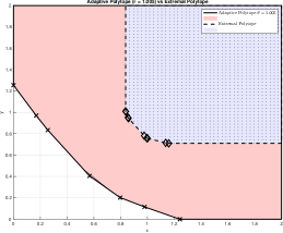
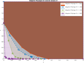
Figure 1. Comparison between extremal and adaptive ($\vartheta=1.005$) polytopes (left). Comparison of adaptive polytopes generated for different values of $\vartheta$ (right).

5.2. Critical example

A critical case for our algorithms is a family $\mathcal{F}$ violating the assumptions of Theorem 6. Specifically, there are secondary eigenvectors lying on the boundary of $\mathbb{R}_{+}^{d}$ and some $A_{i}\in\mathcal{F}$ have non-simple leading eigenvalues. For instance, consider the family $\mathcal{F}=\{A_{1},A_{2}\}$, where

Since $A_{1}$ has a non-simple leading eigenvalue ($\lambda=5$) and $\mathcal{F}$ does not satisfy (8), Theorem 5 does not apply. Thus, the identity (9) fails for an arbitrary antinorm. To illustrate this issue, let $a_{1}(\cdot)$ be the $1$-antinorm. By (17), there holds

$$a_{1}(A_{1})=3\qquad\text{and}\qquad a_{1}(A_{2})=1,$$

which means that the lower bound is $1$ after the first step. It is easy to verify that $a_{1}(A_{2}^{k})=1$ for all $k\in\mathbb{N}$; therefore, the lower bound remains stuck at one, showing that the $1$-antinorm cannot satisfy the Gelfand’s limit (9).

Remark 14.

Even the adaptive algorithms (A) and (E) fail to converge when starting with the $1$-antinorm. This is because vectors with small $2$-norms (order of $10^{-12}$) are incorporated into the vertex set, leading to $S_{6}^{\ast}=\emptyset$. Consequently, no matrix products are selected for evaluation in the subsequent step, preventing the algorithm from progressing further and thus failing to converge to $\delta$.

Since $\check{\rho}(\mathcal{F})=3$ and $\Pi=A_{1}^{3}A_{2}^{4}$ is a s.l.p., we consider the rescaled family $\widetilde{\mathcal{F}}:=\rho(\mathcal{F})^{-1}\cdot\mathcal{F}$ and the vertex set $V=\{v_{1}\}$, where $v_{1}$ is the leading eigenvector of $\widetilde{\Pi}:=\rho(\Pi)^{-1}\cdot\Pi$. In this case, it turns out that:

• Algorithm (S) is no longer stuck, but converges too slowly: it returns a lower bound of $0.889231$ with $M=10^{6}$, making it impractical.

• Algorithm (A) converges to the target accuracy $\delta=10^{-6}$ within $\texttt{n}_{op}=512$ antinorm evaluations. However, the vertex set grows to $1020$ vertices despite the pruning procedure, making the linprog function (solving LP problems) increasingly slower.

• Algorithm (E) fails to return a lower bound because eigenvectors of the form $(\star,0,0,0)^{T}$ are included into the vertex set, causing the algorithm to stop prematurely for the same reason described in Remark 14.

To avoid relying on a priori knowledge of an s.l.p., we can use a regularization technique (see Section 3.3) by introducing small perturbations of the form:

$$\widetilde{\mathcal{F}}_{\varepsilon}^{\Delta}=\widetilde{\mathcal{F}}+\varepsilon\{\Delta_{1},\Delta_{2}\},$$ (23)

where $\varepsilon>0$ and $\Delta_{1},\Delta_{2}$ are non-negative matrices with $\|\Delta_{i}\|_{F}=1$. By Theorem 7, the lower spectral radius is right-continuous; therefore, we have:

$$\lim_{\varepsilon\to 0^{+}}\check{\rho}(\mathcal{F}_{\varepsilon}^{\Delta})=\check{\rho}(\mathcal{F}).$$

The main advantage of this approach is that we can choose the perturbations to ensure that $\widetilde{A}_{1}+\varepsilon\Delta_{1}$ and $\widetilde{A}_{2}+\varepsilon\Delta_{2}$ are strictly positive for all $\varepsilon>0$. By the Perron-Frobenius theorem, this choice guarantees the convergence of our algorithms.

$\varepsilon$	Algorithm (A)		Algorithm (E)
	low.bound	up.bound	low.bound	up.bound
$1\text{\times}{10}^{-3}$	$1.001520$	$1.109109$	$1.028864$	$1.109109$
$1\text{\times}{10}^{-4}$	$0.999286$	$1.046703$	$0.999286$	$1.046703$
$1\text{\times}{10}^{-5}$	$0.997308$	$1.018235$	$0.997517$	$1.018235$
$1\text{\times}{10}^{-6}$	$0.994291$	$1.005660$	$0.994587$	$1.005660$
$1\text{\times}{10}^{-7}$	$0.998546$	$1.001086$	$0.999128$	$1.001086$

Table 3. Algorithms (A) and (E) initialized with the $1$-antinorm. Here Algorithm (E) uses the scaling parameter $\vartheta=1.005$ for simplicity.

Let us now focus on numerical simulation results obtained by applying Algorithm (E) to perturbations of $\mathcal{F}$. In particular, we consider several values of the scaling parameter $\vartheta$ and perturbations of the form (23):

$\vartheta$	$\varepsilon$	low.bound	up.bound	$\#V$	$\ell_{slp}$	$\ell_{opt}$
$1.005$	$1\text{\times}{10}^{-3}$	$1.062580$	$1.101026$	$15$	$12$	$16$
	$1\text{\times}{10}^{-5}$	$1.000000$	$1.016912$	$14$	$7$	$12$
	$1\text{\times}{10}^{-7}$	$0.999271$	$1.000948$	$27$	$7$	$13$
$1.015$	$1\text{\times}{10}^{-3}$	$1.0647885$	$1.104739$	$10$	$7$	$16$
	$1\text{\times}{10}^{-5}$	$1.000000$	$1.017197$	$15$	$7$	$12$
	$1\text{\times}{10}^{-7}$	$0.999271$	$1.000968$	$51$	$7$	$13$
$1.025$	$1\text{\times}{10}^{-3}$	$1.065196$	$1.103720$	$11$	$5$	$16$
	$1\text{\times}{10}^{-5}$	$1.000000$	$1.017378$	$14$	$7$	$12$
	$1\text{\times}{10}^{-7}$	$0.999271$	$1.000994$	$74$	$7$	$13$
$1.035$	$1\text{\times}{10}^{-3}$	$1.069077$	$1.110830$	$15$	$7$	$16$
	$1\text{\times}{10}^{-5}$	$1.000000$	$1.019048$	$15$	$7$	$12$
	$1\text{\times}{10}^{-7}$	$0.999271$	$1.001193$	$86$	$7$	$13$
$1.045$	$1\text{\times}{10}^{-3}$	$1.068030$	$1.110830$	$15$	$7$	$15$
	$1\text{\times}{10}^{-5}$	$1.000000$	$1.019048$	$15$	$7$	$12$
	$1\text{\times}{10}^{-7}$	$0.998857$	$1.001193$	$98$	$7$	$13$

Table 4. Algorithm (E) applied for various values of the scaling parameter $\vartheta$.

We conclude with few interesting observations drawn from this data, specifically in comparison with the results presented in Table 3:

• The s.l.p. degree of $7$ is correctly identified for all $\vartheta$ values when $\varepsilon\leq 10^{-5}$.

• For $\varepsilon\in\{10^{-3},10^{-5}\}$, the impact of $\vartheta$ is minimal. This is further confirmed by the similarity in the number of vertices for different $\vartheta$ values.

• The scaling parameter $\vartheta=1.005$ is optimal in two aspects:

  • It yields the smallest gap between upper and lower bounds for $\varepsilon=10^{-7}$.

  • The resulting adaptive antinorm has the smallest number of vertices.

• For $\varepsilon=10^{-7}$, larger values of $\vartheta$ become problematic. The vertex count grows substantially, while the gap between upper and lower bounds widens.

6. Numerical applications

In this section, we discuss two applications in combinatorial analysis that have already been addressed with the polytopic algorithm in [12, Section 8]. Our goal here is different: we aim to find accurate bounds for the lower spectral radius as efficientlt as possible. Thus, it is not essential to identify extremal antinorms; for instance, as shown in Table 5, adaptive polytopes can have significantly fewer vertices than extremal ones while yielding accurate approximations.

6.1. The density of ones in the Pascal rhombus

The Pascal rhombus is an extension of Pascal’s triangle. Unlike the latter, which is generated by summing adjacent numbers in the above row forming a triangular array, the Pascal rhombus creates a two-dimensional rhomboidal shape array ([10]). The elements of the Pascal rhombus can also be characterized by a linear recurrence relation on polynomials:

$$\begin{cases}p_{n}(x)=(x^{2}+x+1)\cdot p_{n-1}(x)+x^{2}\cdot p_{n-2}(x),&\text{for }n\geq 2,\\ p_{0}(x)=1,\quad p_{1}(x)=x^{2}+x+1.\end{cases}$$

The asymptotic growth of $w_{n}$, which denotes the number of odd coefficients in the polynomial $p_{n}$, as shown in [9], depends on the JSR $\hat{\rho}(\mathcal{F})$ and the LSR $\check{\rho}(\mathcal{F})$ of the matrix family $\mathcal{F}:=\{A_{1},A_{2}\}$, where:

$$A_{1}=\begin{pmatrix}0&1&0&0&0\\ 1&0&2&0&0\\ 0&0&0&0&0\\ 0&1&0&0&1\\ 0&0&0&2&1\end{pmatrix}\qquad\text{and}\qquad A_{2}=\begin{pmatrix}1&0&2&0&0\\ 0&0&0&2&1\\ 1&1&0&0&0\\ 0&0&0&0&0\\ 0&1&0&0&0\end{pmatrix}.$$

While the JSR ($\hat{\rho}(\mathcal{F})=2$) can be easily determined, computing the lower spectral radius is quite challenging. In [12], the polytopic algorithm is employed to determine that $\Pi=A_{1}^{3}A_{2}^{3}$ is a s.l.p., resulting in $\check{\rho}(\mathcal{F})=\rho(\Pi)^{1/6}\approx 1.6376$. We now compare this to the outcomes obtained by applying our algorithms:

• Algorithm (S). Setting $M=10^{4}$ and $\delta=10^{-6}$, and applying Algorithm 1 with the $1$-antinorm to the rescaled family $\widetilde{\mathcal{F}}:=\check{\rho}^{-1}(\mathcal{F})\cdot\{A_{1},A_{2}\}$, yields:

  $$0.9987\leq\check{\rho}(\widetilde{\mathcal{F}})\leq 1.$$

  The upper bound equals one because $M$ is large enough for the algorithm to evaluate products of degree six, $\widetilde{\Pi}:=\rho(\Pi)^{-1}\cdot\Pi$ included. In contrast with the example in Section 5.1, increasing $M$ improves the lower bound:

  $$M=10^{6}\implies(1-\texttt{lower bound})\approx 10^{-4}.$$

  However, the difference between the extremal polytope (which includes $8$ vertices) and the polytope corresponding to the $1$-antinorm slows down convergence as $M$ increases.

• Algorithm (A). Applying the adaptive algorithm using the $1$-antinorm as the initial one, yields a significantly more precise and efficient outcome:

  $$M=500\implies(1-\texttt{lower bound})\approx 10^{-6}=\delta.$$

  The algorithm identifies the s.l.p. degree $\ell_{slp}=6$ correctly. If we apply the algorithm again using the refined antinorm (which has $29$ vertices) as the initial one, we achieve a much higher precision ($\delta=10^{-11}$) within the same amount of antinorm evaluations $\texttt{n}_{op}\approx 50$. In this case, the algorithm correctly returns all cyclic permutations of $\widetilde{\Pi}$ as s.l.p. candidates.

• Algorithm (E). Outperforms Algorithm (A) in terms of speed and accuracy; e.g., it achieves an accuracy of $\delta=10^{-12}$ within $150$ antinorm evaluations.

6.2. Euler binary partition functions

Let $r\geq 2$ integer. The Euler partition function $b(k):=b(r,k)$ is defined as the number of distinct binary representations:

$$k=\sum_{j=0}^{+\infty}d_{j}2^{j},\quad\text{where }d_{j}\in\{0,\ldots,r-1\}\text{ for all }j\in\mathbb{N}.$$

The function’s asymptotic behavior - see [26] for an overview - is characterized in [30], for $r$ odd, via the JSR ($\hat{\rho}$) and LSR ($\check{\rho}$) of a matrix family $\mathcal{F}$ as follows:

$$\limsup_{k\to+\infty}\frac{\log b(k)}{\log k}=\log_{2}\hat{\rho}(\mathcal{F})\qquad\text{and}\qquad\liminf_{k\to+\infty}\frac{\log b(k)}{\log k}=\log_{2}\check{\rho}(\mathcal{F}).$$

More precisely, the family $\mathcal{F}$ is given by two $(r-1)\times(r-1)$ matrices which, for $s\in\{1,2\}$, are defined by the following relation:

$$(A_{s})_{ij}=\begin{cases}1&\text{if }i+2-s\leq 2j\leq i+r-s+1,\\ 0&\text{otherwise}.\end{cases}$$

In [12], the polytopic algorithm demonstrates that for $r$ odd (up to $41$), one of the matrices $A_{1}$ or $A_{1}A_{2}$ acts as a s.m.p. while the other as a s.l.p.

Remark 15.

Algorithm (A) generally performs better than Algorithm (E), as shown by the data in Table 5 and Table 7. This is likely due to Algorithm (E) including several eigenvectors of matrix products of degree $\geq 3$ in the vertex set, which reduces the impact of the leading eigenvector of the s.l.p. ($A_{1}$ or $A_{1}A_{2}$).

In this context, the $1$-antinorm is not recommended as the cone $\mathbb{R}_{+}^{d}$ is not strictly invariant for $\mathcal{F}$. Instead, we use the polytope antinorm corresponding to $V=\{v_{1}\}$, where $v_{1}$ is the leading eigenvector of $A_{1}$. Moreover, since taking $M$ large has limited benefit when the s.l.p. degree is low, a more effective approach is the following:

1. Apply Algorithm (A)/(E) with $M$ small (e.g., $M=10$) to establish a preliminary bound $L\leq\check{\rho}(\mathcal{F})\leq H$. In this case, the upper bound $H$ already coincides with the LSR because the s.l.p. degree is either one or two.

2. To prevent large entries from appearing while exploring long products, use the preliminary lower bound to rescale the family of matrices. In particular, consider the matrix family $\widetilde{\mathcal{F}}:=L^{-1}\cdot\mathcal{F}$.

3. Set $\delta>0$, $j=1$ (iteration count), and $M$. Apply Algorithm (A)/(E) to obtain a new lower bound ($L_{new}$), upper bound ($H_{new}$, which does not improve further in this case) and vertex set ($V_{new}$).

4. Check the stopping criterion:

   $$H_{new}-L_{new}<\delta\qquad\text{or}\qquad\left|L_{new}-L\right|<\delta.$$ (24)

   If (24) is satisfied or $j=\texttt{maxIter}$ (which is fixed a priori), the procedure terminates, returning $(L_{new},H_{new})$. Otherwise, increase $j$ by one, rescale the family with $L_{new}$, set $L=L_{new}$ and $H=H_{new}$, and re-apply Algorithm (A)/(E) starting with the refined antinorm corresponding to $V_{new}$.

In Table 5, we summarize the results obtained by applying this strategy initializing Algorithm (A) with the parameters $M=100$ and $\texttt{maxIter}=20$. It provides a comparison between the vertex count of adaptive polytopes ($\#V_{adap}$) and extremal polytopes ($\#V_{ext}$), the latter taken from [12, Section 8]. The table also includes a time column (T[s]), rounded to the nearest second, showing the algorithm’s efficiency even for higher dimensions.

r	low.bound	up.bound	T[s]	$\#V_{adap}$	$\#V_{ext}$	r	low.bound	up.bound	T[s]	$\#V_{adap}$	$\#V_{ext}$
$7$	$3.490363$	$3.491891$	$78$	$12$	$14$	$25$	$12.499932$	$12.499971$	$393$	$42$	$58$
$9$	$4.493916$	$4.494493$	$200$	$11$	$17$	$27$	$13.499891$	$13.499938$	$354$	$24$	$37$
$11$	$5.496584$	$5.497043$	$349$	$19$	$24$	$29$	$14.499962$	$14.499982$	$344$	$24$	$43$
$13$	$6.498560$	$6.498947$	$335$	$21$	$28$	$31$	$15.499997$	$15.499999$	$302$	$23$	$34$
$15$	$7.499776$	$7.499842$	$261$	$23$	$23$	$33$	$16.499998$	$16.499999$	$289$	$25$	$55$
$17$	$8.499875$	$8.499904$	$260$	$28$	$30$	$35$	$17.499980$	$17.499997$	$310$	$22$	$102$
$19$	$9.499646$	$9.499789$	$340$	$24$	$46$	$37$	$18.499963$	$18.499994$	$341$	$25$	$113$
$21$	$10.499695$	$10.499813$	$372$	$27$	$50$	$39$	$19.499986$	$19.499994$	$292$	$18$	$59$
$23$	$11.499848$	$11.499894$	$317$	$33$	$31$	$41$	$20.499983$	$20.499997$	$336$	$23$	$120$

Table 5. Data obtained applying the procedure above with Algorithm (A) and initial antinorm determined by the leading eigenvector of $A_{1}$.

In conclusion, we make the following observations:

• Reducing the maximum iteration number leads to slightly less precise approximations, but the computational time decreases significantly - see Table 8.

• Since Algorithm (A) restarts with a rescaled matrix family after each iteration, the target accuracy $\delta$ is relative rather than absolute.

• The vertex set corresponding to the extremal antinorm is typically larger than the adaptive one given by Algorithm (A). This difference becomes more significant in higher dimensions - refer to Table 6.

It is worth noting that Algorithm (E) can be applied to very large values of $r$, returning accurate bounds in a short time-frame. For instance:

r	low.bound	up.bound	s.l.p.	$\#V_{adapt}$	$\#V_{extr}$
$251$	$125.4999994835$	$125.5000000000$	$A_{1}A_{2}$	$27$	$24$
$501$	$250.4999998897$	$250.5000000000$	$A_{1}$	$97$	$11$
$751$	$375.4999999117$	$375.5000000000$	$A_{1}A_{2}$	$125$	$5$
$1001$	$500.4998890105$	$500.5000000000$	$A_{1}$	$4$	$11$
$1501$	$750.4999999250$	$750.5000000000$	$A_{1}$	$30$	$7$

Table 6. Algorithm (E) applied to large values of $r$. Comparison between the adaptive polytopes and the extremal polytopes (given by the polytope algorithm).

Our algorithm is able to identify the correct s.l.p. ($A_{1}$ or $A_{1}A_{2}$), while keeping low the number of vertices of the adaptive antinorm. In addition, convergence to $\delta=10^{-6}$ is typically achieved in a few minutes.

Let us now compare Algorithm (E) applied with two different choice of the initial antinorm: the $1$-antinorm and the antinorm derived from the leading eigenvector of $A_{1}$.

	$1$-antinorm			antinorm $V=\{v_{1}\}$
r	low.bound	up.bound	$\#V$	low.bound	up.bound	$\#V$
$7$	$3.491891$	$3.491891$	$62$	$3.491891$	$3.491891$	$38$
$9$	$4.487566$	$4.494493$	$63$	$4.494370$	$4.494493$	$16$
$11$	$5.489837$	$5.497043$	$66$	$5.497043$	$5.497043$	$23$
$13$	$6.479278$	$6.498947$	$67$	$6.495736$	$6.498947$	$36$
$15$	$7.457363$	$7.499842$	$69$	$7.499830$	$7.499842$	$28$
$17$	$8.461750$	$8.499904$	$72$	$8.499888$	$8.499904$	$29$
$19$	$9.458195$	$9.499789$	$74$	$9.499789$	$9.499789$	$126$
$21$	$10.467492$	$10.499813$	$76$	$10.498826$	$10.499813$	$16$
$23$	$11.460798$	$11.499893$	$72$	$11.499856$	$11.499894$	$29$
$25$	$12.450722$	$12.499971$	$80$	$12.499824$	$12.499971$	$17$
$27$	$13.445389$	$13.499938$	$81$	$13.499723$	$13.499938$	$17$
$29$	$14.414215$	$14.499982$	$84$	$14.499089$	$14.499982$	$16$
$31$	$15.380684$	$15.500000$	$80$	$15.499982$	$15.500000$	$17$
$33$	$16.402404$	$16.500000$	$88$	$16.499194$	$16.500000$	$5$
$35$	$17.424716$	$17.499997$	$90$	$17.499432$	$17.499997$	$9$
$37$	$18.431588$	$18.499994$	$92$	$18.499185$	$18.499994$	$19$
$39$	$19.423864$	$19.499994$	$91$	$19.423864$	$19.499994$	$8$
$41$	$20.414314$	$20.499997$	$95$	$20.499542$	$20.499997$	$9$

Table 7. Algorithm (E) with two different choices of the initial antinorm.

1. Algorithm (E) starting with the $1$-antinorm performs poorly. The accuracy decreases significantly as $r$ increases, and in some cases, it takes hours for a standard laptop to achieve such poor results.

2. The other choice is generally more accurate and requires less computational time, though it does not always converge to $\delta=10^{-6}$.

Finally, we apply Algorithm (A) using the same initial antinorm as Table 5, but limiting the computational cost (reducing the number of allowed iterations). The results, presented in Table 8 below, while less precise than Table 5 due to less allowed iterations, remains relatively accurate compared to Table 7:

r	low.bound	up.bound	$\#V_{adp}$	$\#V_{ext}$	r	low.bound	up.bound	$\#V_{adp}$	$\#V_{ext}$
$7$	$3.489753$	$3.491891$	$11$	$14$	$25$	$12.499378$	$12.499971$	$9$	$58$
$9$	$4.492477$	$4.494493$	$12$	$17$	$27$	$13.498726$	$13.499938$	$11$	$37$
$11$	$5.492146$	$5.497043$	$15$	$24$	$29$	$14.499118$	$14.499982$	$11$	$43$
$13$	$6.495201$	$6.498947$	$16$	$28$	$31$	$15.499456$	$15.499999$	$10$	$34$
$15$	$7.498230$	$7.499842$	$11$	$23$	$33$	$16.499702$	$16.499999$	$7$	$55$
$17$	$8.499265$	$8.499904$	$11$	$30$	$35$	$17.499298$	$17.499996$	$11$	$102$
$19$	$9.497710$	$9.499789$	$8$	$46$	$37$	$18.499373$	$18.499994$	$8$	$113$
$21$	$10.497841$	$10.499813$	$8$	$50$	$39$	$19.499542$	$19.499994$	$7$	$59$
$23$	$11.498875$	$11.499894$	$11$	$31$	$41$	$20.499736$	$20.499997$	$8$	$120$

Table 8. Algorithm (A) with $\texttt{maxIter}=8$ and $M=50$.

7. Simulations on randomly generated families

In this section, we examine the performance of Algorithm (E) applied to randomly generated families of matrices, including both full matrices and sparse matrices with several sparsity densities $\rho$. The section is organized as follows:

1. In Section 7.1, we briefly discuss the unsuitability of the non-adaptive algorithm (Algorithm 1) for such classes of matrices.

2. In Section 7.2, we apply Algorithm (E) to randomly generated families with scaling parameter fixed ($\vartheta=1.005$) and examine the results obtained.

3. In Section 7.3, we apply Algorithm (E) to sparse families with low sparsity densities ($\rho\leq 0.25$) using the regularization technique involving perturbations.

4. In Section 7.4, we discuss the choice of the scaling parameter $\vartheta$ for Algorithm (E) by performing a grid-search optimization.

5. In Section 7.5, we consider examples of families including more than two matrices and compare the results obtained.

7.1. Algorithm (S) analysis

Algorithm (S) exhibits limitations when applied to sparse matrices with sparsity density $\rho\leq 0.5$, mainly due to the many zero entries. While it can be utilized for (almost) full matrices, its performance in high-dimensional spaces is poor compared to adaptive algorithms, as shown in the table below:

	$1$-antinorm		antinorm $V=\{v_{1}\}$
d	low.bound	up.bound	low.bound	up.bound
$25$	$12.014676$	$12.204626$	$12.124379$	$12.396828$
$50$	$24.213542$	$24.545062$	$24.267634$	$24.573435$
$100$	$49.671633$	$50.133269$	$49.632976$	$49.632976$
$150$	$74.001873$	$74.530903$	$74.672414$	$75.389293$
$200$	$96.186436$	$100.017694$	$98.924848$	$99.742000$

Table 9. Algorithm (S) with two different choices of the initial antinorm.

All simulations were conducted with a maximum of $M=10^{5}$ antinorm evaluations. This limitation was necessary as high-dimensional cases ($d\geq 50$) required several hours for algorithm termination, especially with the $1$-antinorm.

As expected, using the antinorm given by the leading eigenvector of a matrix family element yielded more accurate results than the $1$-antinorm. However, in no instance did we achieve convergence within a reasonable time-frame, making Algorithm (S) unsuitable for randomly generated families.

Conversely, as shown in subsequent sections, adaptive algorithms significantly outperforms Algorithm (S) in both speed and accuracy.

7.2. Algorithm (E) analysis

We now examine the performance of Algorithm (E) applied with $\vartheta=1.005$ to randomly generated families of matrices, including both full matrices and sparse matrices with several sparsity densities $\rho$.

Remark 16.

For randomly generated families, the s.l.p. degree is typically small; thus, we employ the same strategy outlined in Section 6.2.

d	low.bound	up.bound	$(\ell_{slp},\ell_{opt},\texttt{n},\texttt{n}_{op},\texttt{J}_{max})$	$\#V$	T[s]
$25$	$12.555472$	$12.555472$	$(1,3,3,14,8)$	$4$	$46$
$25$	$12.228911$	$12.228911$	$(2,7,7,254,128)$	$30$	$108$
$50$	$24.647721$	$24.647721$	$(1,3,3,14,8)$	$12$	$32$
$50$	$24.792006$	$24.792006$	$(3,5,5,62,32)$	$4$	$38$
$100$	$49.419854$	$49.419909$	$(3,5,7,254,128)$	$4$	$78$
$100$	$49.660798$	$49.660798$	$(1,2,2,6,4)$	$32$	$118$
$150$	$74.813865$	$74.813865$	$(1,6,6,126,64)$	$4$	$39$
$150$	$74.883378$	$74.883379$	$(1,3,3,14,8)$	$4$	$82$
$200$	$100.172004$	$100.172005$	$(3,11,11,154,20)$	$5$	$32$
$200$	$99.915573$	$99.915574$	$(1,5,5,62,32)$	$4$	$51$

Table 10. Algorithm (E) applied to randomly generated families of strictly positive matrices. The initial antinorm is given by the leading eigenvector of $A_{1}$.

As shown in Table 10, Algorithm (E) establishes bounds for the LSR of $d\times d$ random families with strictly nonzero entries, achieving high accuracy.

The efficiency of the algorithm is demonstrated by low values of $\texttt{J}_{max}$, which represents the maximum number of factors evaluated at any degree. When the set of examined products $S_{k}^{\ast}$ remains small, the algorithm can analyze longer matrix products within a small number of antinorm evaluations (e.g., $M=200$). Furthermore, the adaptive procedure typically adds only a few vertices to the initial antinorm, keeping the computational cost reasonable while improving the convergence rate.

Interestingly, the algorithm correctly identified a s.l.p. in most cases (except for the first $200\times 200$ family), which we verified using the polytopic algorithm.

$\rho$	d	low.bound	up.bound	$(\ell_{slp},\ell_{opt},\texttt{n},\texttt{n}_{op},\texttt{J}_{max})$	$\#V$
$0.25$	$25$	$2.531959$	$2.531959$	$(3,7,7,254,128)$	$8$
	$50$	$5.425970$	$5.425970$	$(2,8,8,510,256)$	$29$
	$100$	$11.22993$	$11.22993$	$(2,6,6,126,64)$	$19$
	$150$	$16.338661$	$16.338661$	$(2,8,8,510,256)$	$8$
	$200$	$22.194604$	$22.194604$	$(2,4,4,30,16)$	$8$
$0.50$	$25$	$4.700123$	$4.700123$	$(4,6,6,126,64)$	$13$
	$50$	$9.771280$	$9.771280$	$(3,4,4,30,16)$	$4$
	$100$	$19.748468$	$19.748468$	$(1,4,4,30,16)$	$7$
	$150$	$29.331904$	$29.331904$	$(2,7,7,254,128)$	$7$
	$200$	$39.459047$	$39.459047$	$(2,6,6,126,64)$	$12$
$0.75$	$25$	$6.480977$	$6.480977$	$(2,6,6,126,64)$	$4$
	$50$	$12.811969$	$12.811969$	$(1,5,5,62,32)$	$4$
	$100$	$26.476497$	$26.476497$	$(2,5,5,62,32)$	$4$
	$150$	$39.447342$	$39.447342$	$(1,6,6,126,64)$	$4$
	$200$	$52.924237$	$52.924237$	$(1,4,4,30,16)$	$4$

Table 11. Algorithm (E) applied to randomly generated families of matrices with sparsity density $\rho$. The initial antinorm is given by the leading eigenvector of $A_{1}$.

Table 11 gathers the results obtained when applying the same procedure on sparse matrices with sparsity density $\rho$. Below, we remark some interesting observations:

• For both full and sparse families, we use the initial antinorm given by the leading eigenvector of $A_{1}$. This choice is especially important for sparse matrices, as the $1$-antinorm is not suitable with numerous zero entries.

• When $\rho=0.25$, the algorithm typically incorporates more vertices compared to higher density or full matrices. Furthermore, a relative accuracy of $\delta=10^{-6}$ generally requires a higher number of operations ($\texttt{n}_{op}$). This is likely due to $S_{k}^{\ast}$, which represents the set of matrix products of degree $k$ that are evaluated, having cardinality close to $\Sigma_{k}$. Nonetheless, the algorithm converges within a reasonable time frame and successfully identifies s.l.p. in all tested dimensions $d$.

• When $\rho\in\{0.5,0.75\}$, the algorithm exhibits significantly faster convergence and incorporates fewer vertices.

7.3. Regularization

In this section, we apply Algorithm (E) to families regularized through perturbations, utilizing the methodology outlined in Section 6.2. We focus our analysis on sparse families with low sparsity densities ($\rho\leq 0.25$) and compare the results to Section 7.2, where no regularization technique was used.

d	$\varepsilon$	low.bound	up.bound	$\#V$	$\ell_{slp}$	$\ell_{opt}$
$25$	$1\text{\times}{10}^{-3}$	$0.773553$	$0.773554$	$38$	$4$	$14$
	$1\text{\times}{10}^{-5}$	$0.772502$	$0.772503$	$46$	$1$	$16$
	$1\text{\times}{10}^{-7}$	$0.772492$	$0.772493$	$43$	$1$	$42$
$50$	$1\text{\times}{10}^{-3}$	$2.223289$	$2.223293$	$52$	$1$	$11$
	$1\text{\times}{10}^{-5}$	$2.222668$	$2.222702$	$59$	$1$	$9$
	$1\text{\times}{10}^{-7}$	$2.222460$	$2.222696$	$52$	$1$	$9$
$100$	$1\text{\times}{10}^{-3}$	$4.608453$	$4.608458$	$55$	$3$	$10$
	$1\text{\times}{10}^{-5}$	$4.606516$	$4.607851$	$47$	$3$	$9$
	$1\text{\times}{10}^{-7}$	$4.607840$	$4.607845$	$57$	$3$	$10$
$200$	$1\text{\times}{10}^{-3}$	$9.476520$	$9.476530$	$8$	$2$	$21$
	$1\text{\times}{10}^{-5}$	$9.475914$	$9.475924$	$8$	$3$	$9$
	$1\text{\times}{10}^{-7}$	$9.475908$	$9.475918$	$10$	$1$	$13$

Table 12. Sparse families with sparsity density $\rho=0.10$. Algorithm (E) is applied starting from the leading eigenvector of $A_{1}$.

Remark 17.

Let us make a few observations about the data gathered above:

• Optimizing the scaling parameter $\vartheta$ is not a concern here. Thus, we use the fixed value $\vartheta=1.010$ for all simulations for consistency.

• Due to the low sparsity density, the $1$-antinorm is not suitable to initialize the algorithm as it may get stuck. Instead, we use the polytope antinorm derived from the leading eigenvector of $A_{1}$.

We now make a few observations about the data gathered in Table 12. In this case, we know that the LSR is right-continuous, so we expect that

$$\check{\rho}(\mathcal{F})\approx\check{\rho}(\mathcal{F}_{\varepsilon})$$

with $\varepsilon=10^{-7}$ is the correct approximation with a target accuracy of $\delta=10^{-6}$. In other words, a natural question arising here is the following: is it true that

$$\check{\rho}(\mathcal{F}_{\varepsilon})=\check{\rho}(\mathcal{F})+C\varepsilon+\mathcal{O}(\varepsilon^{2})$$ (25)

for some positive constant $C$? Another interesting question is the following: if the matrix product $\Pi_{\varepsilon}=\prod_{j=1}^{k}(A_{i_{j}}+\varepsilon\Delta_{i_{j}})$ is a s.l.p. for $\mathcal{F}_{\varepsilon}$, is it true that

$$\Pi:=\Pi_{\varepsilon}\,\big{|}_{\varepsilon=0}=\prod_{j=1}^{k}\left(A_{i_{j}}+\varepsilon\Delta_{i_{j}}\right)\,\Big{|}_{\varepsilon=0}=\prod_{j=1}^{k}A_{i_{j}}$$

is a s.l.p. for the unperturbed family $\mathcal{F}$? For example, when $d=25$ and $\varepsilon=10^{-7}$, the algorithm finds the s.l.p.

$$\Pi_{10^{-7}}=A_{1}+10^{-7}\Delta_{1}.$$

Next, we apply the polytopic algorithm to $\Pi=A_{1}$ and $\mathcal{F}$ and find that $\Pi$ is indeed a s.l.p. for the unperturbed family $\mathcal{F}$ and the extremal antinorm consists of $71$ vertices. As a result, the LSR of $\mathcal{F}$ can be computed exactly as $\check{\rho}(\mathcal{F})=\rho(A_{1})$. Thus,

$$\check{\rho}(\mathcal{F}_{\varepsilon})-\check{\rho}(\mathcal{F})=\rho(A_{1}+\varepsilon\Delta_{1})-\rho(A_{1})\approx\varepsilon$$

holds when $\varepsilon=10^{-7}$, which means that (25) is verified in this case, making this approximation correct for a target accuracy of $\delta=10^{-6}$.

In conclusion, the regularization technique performs well for any value of the dimension $d$ tested. The target accuracy of $\delta=10^{-6}$ is achieved within minutes, while the number of vertices remains relatively small.

d	$\varepsilon$	low.bound	up.bound	T[s]	$\#V$	$\ell_{slp}$	$\ell_{opt}$
$25$	$1\text{\times}{10}^{-3}$	$2.293235$	$2.293237$	$120$	$22$	$6$	$10$
	$1\text{\times}{10}^{-5}$	$2.292609$	$2.292612$	$93$	$24$	$4$	$7$
	$1\text{\times}{10}^{-7}$	$2.292603$	$2.292605$	$80$	$26$	$2$	$8$
$50$	$1\text{\times}{10}^{-3}$	$4.484785$	$4.484790$	$56$	$15$	$1$	$8$
	$1\text{\times}{10}^{-5}$	$4.484173$	$4.484177$	$70$	$18$	$1$	$7$
	$1\text{\times}{10}^{-7}$	$4.484167$	$4.484171$	$74$	$20$	$2$	$7$
$100$	$1\text{\times}{10}^{-3}$	$4.608453$	$4.608458$	$40$	$55$	$3$	$10$
	$1\text{\times}{10}^{-5}$	$4.606516$	$4.607851$	$45$	$47$	$3$	$9$
	$1\text{\times}{10}^{-7}$	$4.607840$	$4.607845$	$32$	$57$	$3$	$10$
$200$	$1\text{\times}{10}^{-3}$	$17.940780$	$17.940797$	$120$	$9$	$3$	$8$
	$1\text{\times}{10}^{-5}$	$17.940174$	$17.940191$	$131$	$10$	$2$	$7$
	$1\text{\times}{10}^{-7}$	$17.940167$	$17.940185$	$176$	$10$	$2$	$10$

Table 13. Regularization of sparse families with sparsity density $\rho=0.20$.

The results for a sparsity density of $\rho=0.2$ show a marked improvement in both accuracy and computational efficiency compared to those presented in Table 12.

Additionally, if we examine closely the case of $d=50$, we see that the algorithm returns the following s.l.p. candidates depending on the value of $\varepsilon$:

$$\Pi_{\varepsilon}=\begin{cases}A_{2}+\varepsilon\Delta_{2}&\text{for }\varepsilon\in\{10^{-3},10^{-5}\},\\ (A_{2}+\varepsilon\Delta_{2})^{2}&\text{for }\varepsilon=10^{-7}.\end{cases}$$

Theoretically, given that the spectral radius property $\rho(A^{2})=\rho(A)^{2}$ holds for any matrix $A$, the algorithm should have returned $A+\varepsilon\Delta_{2}$ for all $\varepsilon$ tested. The observed discrepancy for $\varepsilon=10^{-7}$ is likely due to numerical inaccuracies in computing the square root, which updates the upper bound even though it does not change.

That said, we applied the polytopic algorithm to $A_{2}$ directly. This confirmed that $A_{2}$ is indeed a s.l.p. for the unperturbed family. The extremal antinorm for this case has only $9$ vertices, which is fewer than all the adaptive ones.

d	$\varepsilon$	low.bound	up.bound	T[s]	$\#V$	$\ell_{slp}$	$\ell_{opt}$
$50$	$1\text{\times}{10}^{-3}$	$5.585884$	$5.585890$	$50$	$12$	$1$	$9$
	$1\text{\times}{10}^{-5}$	$5.585274$	$5.585280$	$55$	$11$	$1$	$13$
	$1\text{\times}{10}^{-7}$	$5.585268$	$5.585274$	$64$	$11$	$1$	$5$
$100$	$1\text{\times}{10}^{-3}$	$10.853029$	$10.853039$	$165$	$14$	$5$	$10$
	$1\text{\times}{10}^{-5}$	$10.852423$	$10.852434$	$268$	$14$	$1$	$5$
	$1\text{\times}{10}^{-7}$	$10.852417$	$10.852428$	$462$	$14$	$3$	$7$
$150$	$1\text{\times}{10}^{-3}$	$16.593939$	$16.593956$	$239$	$12$	$3$	$9$
	$1\text{\times}{10}^{-5}$	$16.593333$	$16.593349$	$136$	$13$	$1$	$11$
	$1\text{\times}{10}^{-7}$	$16.593326$	$16.593343$	$353$	$13$	$1$	$5$

Table 14. Regularization of sparse families with sparsity density $\rho=0.25$.

Comparing the data in Table 14 with Table 11, we deduce that the regularization technique does not yield better performances for a sparsity density of $\rho=0.25$. This suggests that at this density level, the matrices structure is robust enough to make perturbations essentially useless.

Therefore, for sparsity densities $\rho\geq 0.25$, Algorithm (E) can generally be applied directly without the need for regularization, thus improving computational efficiency.

7.4. Optimization of the scaling parameter

In this section, we discuss the choice of the scaling parameter $\vartheta$ for Algorithm (E). In particular, we focus on two classes of matrices in relatively high dimensions: full and sparse matrices.

• For consistency, we initialize the algorithm with the antinorm derived from the leading eigenvalue of $A_{1}$ for both classes.

• Since from a theoretical point of view there is no information on optimal values of $\vartheta$, we employ a grid-search strategy in Table 15 and Table 16.

d	$\vartheta$	low.bound	up.bound	$\ell_{slp}$	$\ell_{opt}$	$\texttt{n}_{op}$	$\texttt{J}_{max}$	$\#V$
$50$	$1.0005$	$24.4721163$	$24.4721163$	$1$	$8$	$26$	$3$	$2$
	$1.0010$	$24.4721163$	$24.4721163$	$1$	$8$	$26$	$3$	$2$
	$1.0050$	$24.4721163$	$24.4721163$	$1$	$8$	$26$	$3$	$2$
	$1.0100$	$24.4721163$	$24.4721163$	$1$	$12$	$58$	$4$	$2$
	$1.0200$	$24.4721163$	$24.4721163$	$1$	$12$	$58$	$4$	$2$
	$1.0500$	$24.4721163$	$24.4721163$	$1$	$8$	$26$	$3$	$2$
	$1.1000$	$24.4721163$	$24.4721163$	$1$	$8$	$26$	$3$	$2$
	$1.5000$	$24.4721163$	$24.4721163$	$1$	$8$	$26$	$3$	$3$
	$1.8000$	$24.4721163$	$24.4721163$	$1$	$5$	$20$	$3$	$2$
$150$	$1.0005$	$75.1124947$	$75.1124947$	$1$	$7$	$16$	$2$	$4$
	$1.0010$	$75.1124947$	$75.1124947$	$1$	$7$	$16$	$2$	$3$
	$1.0050$	$75.1124947$	$75.1124947$	$1$	$7$	$16$	$2$	$3$
	$1.0100$	$75.1124947$	$75.1124947$	$1$	$7$	$20$	$2$	$3$
	$1.0200$	$75.1124947$	$75.1124947$	$1$	$7$	$20$	$2$	$4$
	$1.0500$	$75.1124947$	$75.1124947$	$1$	$7$	$20$	$2$	$4$
	$1.1000$	$75.1124947$	$75.1124947$	$1$	$6$	$18$	$2$	$2$
	$1.5000$	$75.1124947$	$75.1124947$	$1$	$7$	$20$	$2$	$3$
	$1.8000$	$75.1124947$	$75.1124947$	$1$	$7$	$20$	$2$	$3$

Table 15. Algorithm (E) applied for different values of $\vartheta$ to full matrix families.

The behavior for full matrices yields unexpected results, as the value of $\vartheta$ appears to have minimal impact on perfomance. More precisely, referring to Table 15, we observe that:

1. In both dimensions tested, the algorithm converges quickly to the target accuracy $\delta=10^{-6}$, regardless of the $\vartheta$ value used.

2. ($d=50$) The algorithm correctly identifies the s.l.p. degree as $1$. The matrix $A_{2}$ is confirmed to be a s.l.p. by the polytopic algorithm, with its extremal antinorm having $4$ vertices. Therefore, the LSR of $\mathcal{F}$ is:

   $$\check{\rho}(\mathcal{F})=\rho(A_{2})\approx 24.4721163.$$

   The algorithm is extremely efficient, exploring products up to degree $12$ within fewer than $100$ antinorm evaluations ($\texttt{n}_{op}$). Indeed, the low values of $\texttt{J}_{max}$ indicate that each $S_{k}^{\ast}$ contains only a few elements - refer to Theorem 6 and Proposition 4 for the precise notations used here.

3. ($d=100$) As above, convergence to $\delta=10^{-6}$ is achieved quickly, and the correct s.l.p. degree is identified. This results in the following equality:

   $$\check{\rho}(\mathcal{F})=\rho(A_{2})\approx 75.1124947.$$

   Efficiency is even more significant in this case, with at most $\texttt{n}_{op}=20$ antinorm evaluations required for convergence.

Remark 18.

The convergence appears to be independent of the $\vartheta$ value tested. This unexpected behavior may be attributed to the adaptive procedure incorporating only a few new vertices, reducing the overall impact of $\vartheta$.

d	$\vartheta$	low.bound	up.bound	$\ell_{slp}$	$\ell_{opt}$	$\texttt{n}_{op}$	$\texttt{J}_{max}$	$\#V$
$100$	$1.0005$	$12.8611170$	$12.8611170$	$2$	$11$	$66$	$4$	$7$
	$1.0050$	$12.8611170$	$12.8611170$	$2$	$11$	$66$	$4$	$7$
	$1.0150$	$12.8611170$	$12.8611170$	$2$	$11$	$66$	$4$	$6$
	$1.0500$	$12.8611170$	$12.8611170$	$2$	$7$	$32$	$3$	$6$
	$1.5000$	$12.8611170$	$12.8611170$	$2$	$7$	$32$	$3$	$4$
$150$	$1.0005$	$19.5415187$	$19.5415187$	$1$	$4$	$12$	$2$	$11$
	$1.0050$	$19.5415187$	$19.5415187$	$1$	$4$	$12$	$2$	$11$
	$1.0150$	$19.5415187$	$19.5415187$	$1$	$4$	$12$	$2$	$11$
	$1.0500$	$19.5415187$	$19.5415187$	$1$	$4$	$12$	$2$	$11$
	$1.5000$	$19.5415187$	$19.5415187$	$1$	$4$	$12$	$2$	$11$

Table 16. Algorithm (E) applied to sparse matrices with sparsity density $\rho=0.3$.

Analysis of Table 16 shows that Algorithm (E) performs well when applied to sparse matrices with a sparsity density of $\rho=0.3$. A few conclusive observations:

1. ($d=100$) The algorithm converges quickly to the target accuracy $\delta=10^{-6}$ and returns $\ell_{slp}=2$. The candidate s.l.p. identified is $\Pi=A_{1}A_{2}$, which is confirmed to be a s.l.p. for $\mathcal{F}$ by the polytopic algorithm. Hence:

   $$\check{\rho}(\mathcal{F})=\rho(A_{1}A_{2})^{1/2}\approx 12.8611169884195,$$

   with an extremal antinorm that has $14$ vertices. As in Table 15, the algorithm is rather efficient, exploring relatively long products within few antinorm evaluations.

2. ($d=150$) The algorithm converges quickly, returning $\ell_{slp}=1$. The polytopic algorithm confirms that $A_{1}$ is a s.l.p., and hence

   $$\check{\rho}(\mathcal{F})=\rho(A_{1})\approx 19.5415186589294.$$

   The extremal antinorm has only $8$ vertices, fewer than our adaptive ones.

Remark 19.

The value of $\vartheta$ appears to have no impact on the result. This is due to no eigenvectors surviving the pruning procedure, likely due to the initial antinorm including the leading eigenvector of the s.l.p. $A_{1}$.

7.5. Random families of several matrices

The results, in the case of families including more than two matrices, are consistent with what we have observed so far: convergence to the pre-fixed accuracy $\delta$ is achieved in a reasonable time and, generally, s.l.p. are identified correctly. A few examples are detailed below:

1. Let $\mathcal{F}=\{A_{1},A_{2},A_{3}\}$, where each $A_{i}$ is a $50\times 50$ matrix with all strictly positive entries. Applying Algorithm (E) with $\vartheta=1.005$, yields:

   $$24.5734346483858\leq\check{\rho}(\mathcal{F})\leq 24.5734346483858.$$

   The process is rather efficient, as suggested by the low computational time of about ten minutes and the performance metric (Remark 8):

   $$\texttt{p}=(\ell_{slp},\ell_{opt},\texttt{n},\texttt{n}_{op},\texttt{J}_{max})=(1,6,6,1092,729).$$

   The algorithm identifies a candidate of degree $\ell_{slp}=1$ ($A_{1}$), which is confirmed to be a s.l.p. with the polytopic algorithm; consequently,

   $$\check{\rho}(\mathcal{F})=\rho(A_{1})\approx 24.5734346483858.$$

2. Let $\mathcal{F}=\{A_{1},A_{2},A_{3}\}$, where each $A_{i}$ is a $200\times 200$ matrix with all strictly positive entries. Applying Algorithm (E) with $\vartheta=1.005$ leads to

   $$100.094951113593\leq\check{\rho}(\mathcal{F})\leq 100.095037706193,$$

   Therefore, convergence is achieved with absolute accuracy $\delta_{abs}=10^{-4}$ and relative accuracy $\delta=10^{-6}$. The metric performance is

   $$\texttt{p}=(\ell_{slp},\ell_{opt},\texttt{n},\texttt{n}_{op},\texttt{J}_{max})=(1,6,6,1092,729)$$

   returning a unique s.l.p. candidate of degree one, $A_{3}$, that is confirmed to be a s.l.p. with the polytopic algorithm; thus,

   $$\check{\rho}(\mathcal{F})=\rho(A_{3})\approx 100.095037706193.$$

3. Let $\mathcal{F}=\{A_{1},A_{2},A_{3},A_{4}\}$ be a family of $150\times 150$ sparse matrices with sparsity density $\rho=0.5$. Applying Algorithm (E) with $\vartheta=1.005$, yields:

   $$29.2101076342739\leq\check{\rho}(\mathcal{F})\leq 29.2608364813336.$$

   Thus, the algorithm does not converge within the allowed number of antinorm evaluations to $\delta=10^{-6}$. Nevertheless, the performance metric is

   $$\texttt{p}=(\ell_{slp},\ell_{opt},\texttt{n},\texttt{n}_{op},\texttt{J}_{max})=(1,5,5,1364,1024).$$

   and there is a unique s.l.p. candidate of degree one, $\Pi:=A_{3}$. The polytopic algorithm converges in four iterations and confirms that

   • $\Pi$ is an actual s.l.p. for $\mathcal{F}$;

   • the extremal antinorm consists of $35$ vertices.

8. Conclusive remarks

In this article, we have extended Gripenberg’s algorithm for the first time to approximate the lower spectral radius for a class of families of matrices. This can be efficiently coupled with the polytope algorithm proposed in [12] when an exact computation is needed. However, being significantly faster than the polytope algorithm, in applications where an approximation of the lower spectral radius suffices, our algorithm can replace the polytope algorithm. We have analyzed several versions of the algorithm and in particular, beyond a standard basic formulation, we have considered and extensively experimented two main variations: an adaptive one, utilizing different antinorms, and a second one exploiting the knowledge of eigenvectors of certain products in the matrix semigroup. Further variants might be successfully explored for specific kind of problems. The algorithms are publically available and will hopefully be useful to the community, particularly for their relevance in important applications in approximation theory and stability of dynamical systems.

Finally, we briefly discuss in the next subsection an adaptive Gripenberg’s algorithm for the joint spectral radius computation. This extension of the original algorithm uses ideas similar to those proposed for approximating of the lower spectral radius. The obtained results indicate the advantages of using an adaptive strategy.

8.1. Adaptive Gripenberg’s algorithm for the JSR

The adaptive procedure used in Algorithm (A) suggests that a similar improvement can be implemented in Gripenberg’s algorithm [11]. First, we recall a few definitions from [12, 15, 35]:

Definition 16.

A set $P\subset\mathbb{C}^{d}$ is a balanced complex polytope (b.c.p.) if there exists a minimal set of vertices $V=\{v_{1},\ldots,v_{p}\}$ such that

$$\operatorname{span}(V)=\mathbb{C}^{d}\qquad\text{and}\qquad P=\operatorname{absco}(V),$$

where $\operatorname{absco}(\cdot)$ denotes the absolute convex hull. Moreover, a complex polytope norm is any norm $\|\cdot\|_{P}$ whose unit ball is a b.c.p. $P$.

Complex polytope norms are dense in the set of all norms on $\mathbb{C}^{d}$. This property extends to the induced matrix norms (see [15]). Consequently, we have:

$$\hat{\rho}(\mathcal{F})=\inf_{\|\cdot\|_{P}}\max_{A\in\mathcal{F}}\|A\|_{P}.$$

Therefore, even though an extremal complex polytope norm for $\mathcal{F}$ may not exist, the density property allows an arbitrarily close approximation of the JSR.

The numerical implementation is similar to Algorithm (A), but there are two crucial differences: how to compute $\|\cdot\|_{P}$ and when to add new vertices. Indeed, if we consider $P=\operatorname{absco}(V)$, then $\|z\|_{P}$ is given by the solution to

$$\max t_{0}\qquad\text{subject to }\begin{cases}\sum_{x\in V}\alpha_{x}\text{Re}(x)-\beta_{x}\text{Im}(x)=t_{0}\text{Re}(z)\\[3.99994pt] \sum_{x\in V}\beta_{x}\text{Re}(x)+\alpha_{x}\text{Im}(x)=t_{0}\text{Im}(z)\\[3.99994pt] \sum_{x\in V}\sqrt{\alpha_{x}^{2}+\beta_{x}^{2}}\leq 1\end{cases}$$ (26)

This optimization problem can be solved in the framework of the conic quadratic programming; for more details, refer to [12]. The decision to include $z$ in the vertex set relies on the same criterion of Algorithm (A), but with a reversed inequality. More precisely

• if $t_{0}>1$, then $z$ falls outside the polytope (so we discard it);

• if $t_{0}\leq 1$, then $z$ is incorporated into the vertex set.

Example of the adaptive Gripenberg algorithm

Consider the family:

$$\mathcal{F}=\frac{1}{5}\left\{\begin{pmatrix}3&0\\ 1&3\end{pmatrix},\begin{pmatrix}3&-3\\ 0&-1\end{pmatrix}\right\}.$$

In [11], numerical simulations (on MATLAB) with a maximum number of norm computations $M=52550$ yielded the following bound: $0.6596789<\hat{\rho}(\mathcal{F})<0.6596924$.

In this case, the algorithm considers products of length up to $243$ using the $2$-norm. It is also mentioned that increasing the value of $M$ does not improve the bound.

Applying the adaptive Gripenberg algorithm with the $1$-norm and setting $M=250$ yields (in about ten minutes) the following upper bound:

$$\hat{\rho}(\mathcal{F})\leq 0.659678900000002.$$

This is obtained exploring products of length up to eight, however the optimal gap is achieved at $3$. Additionally, only three vertices are added to the initial $1$-norm.

Remark 20.

The lower bound does not improve as the spectral radius does not benefit from this adaptive procedure.

Appendix A Polytopic antinorms

Let $\mathcal{F}$ be a finite family of real non-negative $d\times d$ matrices sharing an invariant cone $K\subseteq\mathbb{R}_{+}^{d}$. Consider a polytope antinorm

$$a(\cdot):K\longrightarrow\mathbb{R}_{+},$$

and let $V=\{v_{1},\ldots,v_{p}\}$ be a minimal vertex set for $a(\cdot)$. For any product $P\in\Sigma(\mathcal{F})$, we can compute its antinorm using the following formula:

$$a(P):=\min_{1\leq i\leq p}a(Pv_{i}).$$ (27)

Thus, being able to calculate $a(z)$ efficiently for any $z$ is fundamental. As mentioned in Section 4.2, this can be done by solving the LP problem (19). Since our algorithm relies on the linprog built-in MATLAB function, let us briefly summarize the key points and introduce some relavant notation for Algorithm 2:

1. The function linprog only solves LP problems of the form

   $$\min_{x\in\mathbb{R}^{N}}f^{T}x\qquad\text{ subject to }\begin{cases}Ax\leq b,\\ A_{eq}x=b_{eq},\\ l_{b}\leq x\leq u_{b}.\end{cases}$$

   Therefore, to write (19) in this form, we take $f=(1,0,\ldots,0)^{T}\in\mathbb{R}^{p+1}$ and we let $x$ be the vector $(c_{0},c_{1},\ldots,c_{p})\in\mathbb{R}^{p+1}$. The inequality constraints

   $$c_{0}z\geq\sum_{i=1}^{p}c_{i}v_{i}\qquad\text{and}\qquad\sum_{i=1}^{p}c_{i}\geq 1$$

   must be written as $Ax\leq b$. Hence, we take $b=(0,\ldots,0,-1)^{T}\in\mathbb{R}^{d+1}$ and define the augmented matrix:

   $$A=\begin{pmatrix}-z_{1}&|&\lx@intercol\hfil\hfil\lx@intercol&\\ \vdots&|&\lx@intercol\hfil\vspace{\jot}V\hfil\lx@intercol&\\ -z_{d}&|&\lx@intercol\vspace{\jot}\hfil\hfil\lx@intercol&\\ \cline{1-5}\cr 0&|&-1&\ldots&-1\end{pmatrix}\in\mathbb{R}^{(d+1),(p+1)}.$$ (28)

   The last constraint, $c_{i}\geq 0$ for each $i$, is recovered by setting $l_{b}=(0,\ldots,0)^{T}\in\mathbb{R}^{p+1}$ and leaving $u_{b}$ empty to indicate that there are no upper bounds on the variables. Notice also that the optimization problem (19) has no equality constraints, so we simply let $A_{eq}$ and $b_{eq}$ be empty.

2. To better suit our problem, we customize some options of linprog:

   • algorithm: The method used to find the solution. We use the interior-point algorithm since it works well with linear problems.

   • maxIter: Maximum number of iterations allowed; in our case, we set $\max\{300,d\}$ as a reasonable choice for all dimensions.

   • tol: Termination tolerance on the dual feasibility.

3. The implementation requires careful consideration, as it may occasionally fail to return a solution. To address this issue without interrupting the main algorithm (e.g., Algorithm 1), we can utilize the exitflag value returned by linprog as it provides information about the reason for termination.

Algorithm 2 Evaluation of the polytope antinorm $a(\cdot)$ on a vector $z$

1:  Initial data: $z\in K$ and $V=\begin{pmatrix}v_{1}&\cdots&v_{p}\end{pmatrix}$ vertex matrix corresponding to $a(\cdot)$

2:  Setting of the LP problem as in (a) above:

3:  let $f=(1,0,\ldots,0)^{T}\in\mathbb{R}^{p+1}$, $b:=(0,\ldots,0,-1)^{T}\in\mathbb{R}^{d+1}$, and denote by $A$ the augmented matrix given in (28)

4:  set $A_{eq},b_{eq}$ and $u_{b}$ empty and $l_{b}=(0,\ldots,0)^{T}\in\mathbb{R}^{p+1}$

5:  configure linprog’s options by setting $\texttt{tol}=10^{-10}$ and $\texttt{maxIter}=\max\{300,d\}$ {note that ’interior-point’ is the default setting for algorithm}

6:  let $x$ be the solution obtained via linprog {for simplicity, assume that a solution is found; however, in the actual implementation, the value of exitflag should be checked to handle potential errors}

7:  if $x(1)=+\infty$ then

8:     set $a(z)=0$

9:  else if $x(1)=0$ then

10:     set $a(z)=+\infty$

11:  else

12:     set $a(z)=1/x(1)$

13:  end if

14:  return  $a(z)$

We can now exploit the formula (27) to compute the antinorm $a(P)$ of any given product matrix $P\in\Sigma(\mathcal{F})$. Furthermore, since it is used in the adaptive algorithm, Algorithm 3 returns the candidate vertex $z:=Pv_{i}$, where $v_{i}\in V$ achieves the minimum in (27).

Remark 21.

Algorithm (A), detailed in Appendix B, incorporates new vertices immediately if a criterion is satisfied. As a result, Algorithm 3 is applied to each product $P\in S_{k}$ with a potentially different polytope antinorm.

Algorithm 3 Polytope antinorm evaluation at a matrix product $P\in\Sigma(\mathcal{F})$

1:  Initial data: $P\in\Sigma(\mathcal{F})$ and $V=\begin{pmatrix}v_{1}&\cdots&v_{p}\end{pmatrix}$ vertex matrix of $a(\cdot)$

2:  for $i=1$ to $p$ do

3:     compute the product $z_{i}=A\cdot v_{i}$ and its antinorm $a(z_{i})$ with Algorithm 2

4:     store the value in an auxiliary vector $c(i)=a(z_{i})$

5:  end for

6:  set $a(P)=\min_{1\leq i\leq p}c(i)$ and let $j$ be the index such that $a(P)=c(j)$.

7:  return  $a(P)$ and $z:=P\cdot v_{j}$ {i.e., the potential new vertex}

A.1. Vertices pruning

As mentioned in Section 4.2, at the end of each step of the adaptive algorithms, we have an augmented vertex set $V_{aux}$ that is likely not minimal. To address this issue, we employ a pruning procedure before the next algorithm step. However, in Algorithm 4, we need to be careful and avoid:

1. the accidental removal of non-redundant vertices;

2. the same vertex appearing multiple times.

Algorithm 4 Vertices pruning procedure

1:  Initial data: $V=\begin{pmatrix}v_{1}&\cdots&v_{p}\end{pmatrix}$ vertex matrix, $r=0$ {to determine when to stop the procedure} and $\texttt{tol}>0$ {used in the elimination criterion}

2:  while $r$ is equal to $0$ do

3:     let $n_{v}$ be the current number of vertices (i.e, columns) of $V$

4:     if $n_{v}$ is less than or equal to $1$ then

5:        exit the procedure

6:     end if

7:     set $r=1$ {this values is set to zero in the for cycle below if at least one vertex is eliminated; otherwise, it remains one and the while does not restart}

8:     for $i=n_{v},n_{v}-1,\ldots,1$ do

9:        let $v_{i}$ denote the $i$-th column of $V$ and define $W_{i}$ as the matrix obtained by removing the $i$-th column from $V$

10:        if $\operatorname{rank}(W)$ is equal to $1$ then

11:           skip directly to the next index ($i\to i-1$)

12:        end if

13:        compute $a_{W_{i}}(v_{i})$, where $a_{W_{i}}$ is the polytope antinorm with vertex set $W_{i}$

14:        if $a_{W_{i}}(v_{i})\geq 1+\texttt{tol}$ then

15:           set $r=0$ and remove the column $v_{i}$ from $V$, i.e. let $V=W_{i}$

16:        end if

17:     end for

18:  end while

19:  identify all columns of $V$ that appear more than once and remove them

20:  return  $V$

In particular, we examine each $v_{i}$ in the vertex set $V$ by considering the polytope antinorm obtained by excluding $v_{i}$ (which we denote by $a_{W_{i}}$) and, ideally, whenever $v_{i}$ lies on the boundary of said polytope, removing it. However, to avoid removing non-redundant vertices due to numerical inaccuracies, we fix a small tolerance (tol) and use the following inequality as the exclusion criterion:

$$a_{W_{i}}(v_{i})\geq 1+\texttt{tol}.$$

Finally, we make a few remarks about Algorithm 4:

• The stopping criterion $r=1$ halts the procedure as soon as an entire for cycle does not remove any vertex.

• The procedure may be computationally expensive, as a different antinorm $a_{W_{i}}(\cdot)$ appears at each iteartion of the for cycle.

• The fixed tolerance tol should be chosen to be small to maximize the removal of redundant vertices. Setting $\texttt{tol}=0$, while possible, is not recommended, as numerical inaccuracies may lead to the removal of important vertices.

A.2. Identification of s.l.p. candidates

Recall that a product $\Sigma\in\Sigma(\mathcal{F})$ of degree $k$ is a s.l.p. for $\mathcal{F}$ if the following holds:

$$\rho(\Sigma)^{1/k}=\inf_{k\geq 1}\min_{P\in\Sigma_{k}(\mathcal{F})}\rho(P)^{1/k}$$

Referring to the notation of Remark 13, it suffices to calculate $\ell_{slp}$ and then select among products of such degree those minimizing $\rho(P)^{1/\ell_{slp}}$. The numerical implementation is given in Algorithm 5, but first, we summarize the strategy:

1. Set $\ell_{slp}:=1$. Next, enter the main while loop of Algorithm 1 (or any adaptive variant) and complete the step.

2. If the new upper bound is strictly less than the previous value, set $\ell_{slp}$ equal to the current degree. If not, $\ell_{slp}$ remains unchanged.

3. When the algorithm terminates (due to convergence or reaching the maximum number of antinorm evaluations), the value $\ell_{slp}$ coincides with the one given in Remark 13.

4. Solve the minimization problem

   $$\min_{P\in\Sigma_{\ell_{slp}(\mathcal{F})}}\rho(P)^{1/\ell_{slp}},$$

   and apply the polytopic algorithm [12] to all solutions to verify if they are s.l.p.

This procedure can be integrated into any version of the algorithm, but performs better with the adaptive variants. Indeed, a fixed antinorm may lead Algorithm 1 to evaluate a large number of products at each degree and, consequently, limit its ability to explore higher degrees within a reasonable time-frame. In contrast, the adaptive variants consider sets $S_{k}^{\ast}$ with typically smaller cardinality and, hence, take into account higher-degree products at the same computational cost.

There is a potential drawback to this approach: adaptive algorithms might inadvertently remove actual s.l.p.s, resulting in the wrong value for $\ell_{slp}$. Despite this concern, numerical simulations suggest that this is not a common issue.

Remark 22.

A concrete example comparing the performance of Algorithm 1 and (A) and (E) in s.l.p. identification can be found in Section 5.

The numerical implementation of this procedure requires only a few modifications to our algorithms. As such, we will only discuss the lines that should be changed or added, and refer to Algorithm 1 or Algorithm 6 for the complete picture.

Algorithm 5 Identification of s.l.p. candidates

1:  Let $\ell_{slp}$ be the value returned by either Algorithm 1 or Algorithm 6 and do the following:

2:  if $\ell_{slp}$ is small enough then

3:     solve the minimization problem $\min_{P\in\Sigma_{\ell_{slp}}(\mathcal{F})}\rho(P)^{1/\ell_{slp}}$

4:  else if $\ell_{slp}$ is large then

5:     solve the minimization problem $\min_{P\in S_{\ell_{slp}}^{\ast}}\rho(P)^{1/\ell_{slp}}$ {the definition of $S_{\ell_{slp}}^{\ast}$ is given in Proposition 4}

6:  end if

7:  return  all solutions (up to cyclic permutations) of the minimization problem

Appendix B Implementation of Algorithm (A)/(E)

We now present the numerical implementations of the adaptive variants of Algorithm 1: Algorithms (A) and Algorithm (E). For the latter, we only highlight the main differences and omit the complete pseudocode due to their similarity.

Let us examine the complete pseudocode of Algorithm (A). We will maintain the notation from Algorithm 1 whenever possible for clarity.

Remark 23.

The polytope antinorm is defined by its vertex set, which is refined throughout the algorithm. Thus, we use the notation $a_{V}(\cdot)$ to refer to the antinorm corresponding to the current vertex set $V$.

Algorithm 6 Adaptive Algorithm (A)

1:  Set the initial bounds for the lower spectral radius: $L=0$ and $H=+\infty$

2:  Let $S_{1}:=\mathcal{F}$ {to store matrices of degree one, following the notation of Theorem 6} and set $m=\#S_{1}$ {number of elements in the family $\mathcal{F}$}

3:  for $i=1$ to $m$ do

4:     compute $a_{V}(A_{i})$ with Algorithm 3 and let $z_{i}$ be the candidate vertex

5:     set $l(i)=a_{V}(A_{i})$ {the vector $l$ stores all candidates lower bounds in the current step} and $H=\min\{H,\rho(A_{i})\}$ {update the upper bound}

6:     if $a_{V}(z_{i})\leq 1+\texttt{tol}$ then

7:        add $z_{i}$ to the vertex set $V$, i.e. set $V=[V,z_{i}]$

8:     end if

9:  end for

10:  compute the new lower bound as $L=\min_{1\leq i\leq m}l(i)$ and prune the vertex set $V$ by applying Algorithm 4

11:  set $\texttt{n}=1$ {current degree}, $\texttt{n}_{op}=m$ {number of antinorm evaluations}, $\texttt{J}=m$ {cardinality of $S_{\texttt{n}}$, coincides with $m$ after the first step}, and $\texttt{J}_{max}=\texttt{J}$ {keeps track of the maximum value of J}

12:  set $\ell_{opt}=1$ {i.e., the degree for which the gap between lower and upper bounds is optimal} and $\ell_{slp}=1$ {i.e., degree yielding the optimal upper bound}

13:  while $H-L\geq\delta\quad\&\&\quad\texttt{n}_{op}\leq M$ do

14:     set $H_{old}=H$, $L_{old}=L$ and $\texttt{J}_{new}=0$

15:     increase $\texttt{n}=\texttt{n}+1$ and initialize $S_{\texttt{n}}=[\cdot]$ {empty set to store matrix products of degree n for the next iteration, following the notation of Theorem 6}

16:     for $k=1$ to J do

17:        for $i=1$ to $m$ do

18:           let $X_{k}$ be the $k$-th element in $S_{\texttt{n}-1}$ {note: $S_{\texttt{n}-1}$ has cardinality J}

19:           set $q=\texttt{J}_{new}+1$ and consider the product $Y:=X_{k}A_{i}$

20:           compute $a_{V}(Y)$ and let $z_{Y}$ be the candidate vertex

21:           set $l_{new}(q)=\max\{l(k),(a_{V}(Y))^{1/\texttt{n}}\}$ and $H:=\min\{H,(\rho(Y))^{1/\texttt{n}}\}$

22:           if $a_{V}(z_{Y})\leq 1+\texttt{tol}$ then

23:              add $z_{Y}$ to the vertex set $V$, i.e. set $V=[V,z_{Y}]$

24:           end if

25:           if $l_{new}(q)<H-\delta$ then

26:              increase $\texttt{J}_{new}=\texttt{J}_{new}+1$ and compute $L=\min\{L,l_{new}(q)\}$

27:              include $Y$ in the set $S_{\texttt{n}}$ {which will be used in the next iteration}

28:           end if

29:        end for

30:     end for

31:     compute $L=\max\{L_{old},\min\{L,H-\delta\}\}$ and set $l:=l_{new}$

32:     set $\texttt{n}_{op}=\texttt{n}_{op}+\texttt{J}\cdot m$, $\texttt{J}=\texttt{J}_{new}$ and $\texttt{J}_{max}=\max\{\texttt{J},\texttt{J}_{max}\}$

33:     if $H-L<H_{old}-L_{old}$ then

34:        set $\ell_{opt}:=\texttt{n}$ {store the optimal degree so far (for convergence)}

35:     end if

36:     if $H<H_{old}$ then

37:        set $\ell_{slp}:=\texttt{n}$ {store the degree yielding the best upper bound so far}

38:     end if

39:     prune the current vertex set $V$ by applying Algorithm 4

40:  end while

41:  return $\texttt{lsr}:=(L,H)$, $\texttt{p}=(\ell_{opt},\ell_{slp},\texttt{n},\texttt{n}_{op},\texttt{J}_{max})$ and $V$ {final vertex set}

Algorithm (E), on the other hand, has an additional input value: the scaling parameter $\vartheta$. The main changes to Algorithm 6 are the following:

• Modify the first for cycle (lines 3–9). Specifically, store all matrices $A_{j}$ such that in line 5 we have

  $$\min\{H,\rho(A_{j})\}=\rho(A_{j}).$$

  After all elements in $\mathcal{F}$ have been evaluated, before the pruning procedure starts (line 10), find the leading eigenvector $v_{j}$ of each $A_{j}$ stored previously and add to the vertex set $V$ the rescaling

  $$\widetilde{v}_{j}:=v_{j}\left(a_{V}(v_{j})\vartheta\right)^{-1}.$$ (29)

• The same strategy is employed in the main while loop. Specifically, store all matrix products such that

  $$\min\{H,(\rho(Y))^{1/\texttt{n}}\}=(\rho(Y))^{1/\texttt{n}},$$

  and, before the pruning procedure in line $39$, add to $V$ all the leading eigenvectors rescaled as in (29).

Remark 24.

An interesting improvement to this algorithm would be to develop a method for adaptively change the value of $\vartheta$ after each step. The idea is to find a compromise between two conflicting requirements: preventing drastic changes to the antinorm (i.e., $\vartheta$ not too large) and ensuring that the antinorm actually improves (i.e., $\vartheta>1$).

Appendix C Output of Algorithm (A)

We now describe in details the first two steps of Algorithm (A) applied to the example in Section 5.1. Specifically, the input consists of the matrix family already rescaled, i.e.

$$\widetilde{\mathcal{F}}:=\rho(\Pi)^{-1/8}\cdot\left\{\begin{pmatrix}7&0\\ 2&3\end{pmatrix},\begin{pmatrix}2&4\\ 0&8\end{pmatrix}\right\},$$

where $\Pi:=A_{1}A_{2}(A_{1}^{2}A_{2})^{2}$. Fix the accuracy to $\delta=10^{-6}$ and the initial antinorm to $a_{1}(\cdot)$ (the $1$-antinorm), which corresponds to the vertex matrix

$$V_{in}=\begin{pmatrix}1&0\\ 0&1\end{pmatrix}.$$

Step 1: degree-one products (lines 3–9 of Algorithm 6)

The first step only considers the rescaled matrices $\tilde{A}_{1}$ and $\tilde{A}_{2}$ to compute the bounds:

1. The matrix $\tilde{A}_{1}$, when rounded to four decimal digits, is given by

   $$\tilde{A}_{1}\approx\begin{pmatrix}1.1649&0.3328\\ 0&0.4992\end{pmatrix}.$$

   Its $1$-antinorm is $a_{1}(\tilde{A}_{1})=0.8320$, and the candidate vertex returned by Algorithm 3 is $z=(0.3328,0.4992)^{T}$. Recall that $z$ is characterized by

   $$a_{1}(A_{1})=a_{1}(A_{1}z).$$

   Set $l(1):=a_{1}(\tilde{A}_{1})$ (refer to line 6), compute the corresponding spectral radius $\rho(\tilde{A}_{1})=1.1649$ and update the upper bound accordingly:

   $$H=\min\{H,\rho(\tilde{A}_{1})\}=\min\{+\infty,1.1649\}=1.1649.$$

   Store the matrix $\tilde{A}_{1}$ for the next step by setting $S_{1}=\{\tilde{A_{1}}\}$, and go to line 7. Since $a(z)=0.8320$, we add $z$ to the current vertex set:

   $$V=\begin{pmatrix}V_{in}&z\end{pmatrix}=\begin{pmatrix}1&0&0.3328\\ 0&1&0.4992\end{pmatrix}.$$

2. The matrix $\tilde{A}_{2}$, rounded to four decimal places, is given by

   $$\tilde{A}_{2}\approx\begin{pmatrix}0.3328&0\\ 0.6656&1.3313\end{pmatrix}.$$

   Calculate its antinorm with respect to the new vertex set, $a(\tilde{A}_{2})=1.0528$, obtaining the new candidate vertex $z=(0.1108,0.8861)^{T}$. Store its value by setting $l(2)=a(\tilde{A}_{2})$, compute the spectral radius $\rho(\tilde{A}_{2})=1.3313$, and update the upper bound:

   $$H=\min\{H,\rho(\tilde{A}_{2})\}=\min\{1.1649,1.3313\}=1.1649,$$

   which, in this case, does not change. Next, store the matrix $\tilde{A}_{2}$ as follows:

   $$S_{1}=S_{1}\cup\{\tilde{A}_{2}\}=\{\tilde{A}_{1},\tilde{A}_{2}\},$$

   and proceed to line 7. The antinorm of $z$ is $a(z)=1.0528$, so we do not add $z$ to the vertex set, which remains as before:

   $$V=\begin{pmatrix}1&0&0.3328\\ 0&1&0.4992\end{pmatrix}.$$

Pruning, lower bound and iterative parameters

In line 11, compute the lower bound after step one as $\min_{i}l(i)$, which in this case yields:

$$L=\min\{l(1),l(2)\}=l(1)=0.8320.$$

The pruning procedure applied to $V$ does not remove any vertex. Next, proceed to lines 13–14 and initialize the iteration parameters:

$$\texttt{n}=1,\quad\texttt{n}_{op}=2,\quad\texttt{J}=\texttt{J}_{max}=2.$$

Also set $\ell_{opt}=\ell_{slp}=1$ to keep track of the degree yielding the optimal gap and the best (smallest) upper bound respectively.

Step $2$: degree-two products (lines 13–39)

Increase n to $2$ and start the two nested for cycles:

1. When $k=1$ and $i=1$, consider $\tilde{A}_{1}\in S_{1}$ and set $Y=:\tilde{A}_{1}^{2}$, which rounded to the fourth decimal digit is given by

   $$Y\approx\begin{pmatrix}1.3569&0.5538\\ 0&0.2492\end{pmatrix}.$$

   Following line 20, compute the antinorm $a(Y)=0.8869$ to obtain the candidate vertex $z=(0.5538,0.2492)^{T}$ and, then, set

   $$l_{new}(1)=\max\{l(1),a(Y)^{1/2}\}=a(Y)^{1/2}=0.9418.$$

   Compute the spectral radius $\rho(Y)=.3569$, and note that the upper bound cannot improve since $\rho(A^{2})=\rho(A)^{2}$; therefore,

   $$H=\min\{H,\rho(Y)^{1/2}\}=H=\rho(Y)^{1/2}=1.1649.$$

   Next (lines 22–24), establish whether or not $z$ is added to the vertex set. In particular, since $a(z)=0.8869$ is less than $1$, it is incorporated:

   $$V=\begin{pmatrix}1&0&0.3328&0.5538\\ 0&1&0.4992&0.2492\end{pmatrix}.$$

   Finally (line 25), check the condition $l_{new}(1)<H-\delta$. Since it is satisfied, update the lower bound

   $$L=\min\{L,l_{new}(1)\}=l_{new}(1)=0.9418,$$

   and store $Y$ for the next step by setting $S_{2}=\{\tilde{A}_{1}^{2}\}$.

2. When $k=1$ and $i=2$, set $Y:=\tilde{A}_{1}\tilde{A}_{2}$, which rounded to the fourth decimal digit is given by

   $$Y\approx\begin{pmatrix}0.6092&0.4431\\ 0.3323&0.6646\end{pmatrix}.$$

   The antinorm is $a(Y)=0.9778$ and the corresponding candidate vertex is $z=(0.4478,0.3497)^{T}$. Set, once again, the quantity

   $$l_{new}(2)=\max\{l(1),a(Y)^{1/2}\}=a(Y)^{1/2}=0.9888.$$

   The spectral radius of $Y$ is $\rho(Y)=1.0216$ so, since there is an improvement, update the upper bound as follows:

   $$H=\min\{H,\rho(Y)^{1/2}\}=\rho(Y)^{1/2}=1.0108.$$

   Next, establish whether or not $z$ is added to the vertex set. Since $a(z)=0.9778$, the matrix $V$ is updated once again:

   $$V=\begin{pmatrix}1&0&0.3328&0.5538&0.4478\\ 0&1&0.4992&0.2492&0.3497\end{pmatrix}.$$

   Finally, the if condition in line 25 is satisfied; hence, compute the new lower bound as

   $$L=\min\{L,l_{new}(2)\}=l_{new}(2)=0.9418,$$

   and store $Y$ in $S_{2}$ by setting $S_{2}=\{\tilde{A}_{1}^{2},\tilde{A}_{1}\tilde{A}_{2}\}$.

3. When $k=2$ and $i=1$, consider $\tilde{A}_{2}\in S_{1}$ and set $Y=\tilde{A}_{2}\tilde{A}_{1}$, which rounded to the fourth decimal digit is given by

   $$Y\approx\begin{pmatrix}0.3877&0.1108\\ 0.7754&0.8861\end{pmatrix}.$$

   The antinorm of $Y$ is $a(Y)=0.9766$, while the corresponding candidate vertex is $z=(0.2123,0.6571)^{T}$. Set the quantity:

   $$l_{new}(3)=\max\{l(2),a(Y)^{1/2}\}=l(2)=1.0528.$$

   Calculate the spectral radius $\rho(Y)=1.0216$ and notice that the upper bound does not change since $\rho(AB)=\rho(BA)$:

   $$H=\min\{H,\rho(Y)^{1/2}\}=H=\rho(Y)^{1/2}=1.0108.$$

   Next establish whether or not $z$ is added to the vertex set. Since $a(z)=0.9766$ is less than $1$, the matrix $V$ is updated:

   $$V=\begin{pmatrix}1&0&0.3328&0.5538&0.4478&0.2123\\ 0&1&0.4992&0.2492&0.3497&0.6571\end{pmatrix}.$$

   However, the condition in line 25 is not satisfied ($l_{new}(3)>H-\delta$), which means that the product $Y$ is discarded and both the lower bound $L$ and the set $S_{2}$ do not change.

4. When $k=2$ and $i=2$, set $Y:=\tilde{A}_{2}^{2}$, which rounded to the fourth decimal digit is given by

   $$Y\approx\begin{pmatrix}0.1108&0\\ 1.1077&1.7723\end{pmatrix}.$$

   Compute $a(Y)=1.1542$, the candidate vertex $z=(0.0613,1.0552)^{T}$, and set the quantity:

   $$l_{new}(4)=\max\{l(2),a(Y)^{1/2}\}=a(Y)^{1/2}=1.0743.$$

   The spectral radius is $\rho(Y)=1.7723$, so it does not improve the upper bound:

   $$H=\min\{H,\rho(Y)^{1/2}\}=H=1.0108.$$

   Next, since $a(z)=1.1542$, the candidate vertex is discarded. Furthermore, the condition in line 25 is not satisfied ($l_{new}(4)>H-\delta$), so $Y$ is discarded and both $L$ and $S_{2}$ remain unchanged.

Update of iteration parameters and conclusion

Only two products of degree two survived this step since, following the notation of Theorem 6, we have

$$S_{2}=\{\tilde{A}_{1}^{2},\tilde{A}_{1}\tilde{A}_{2}\}.$$

This set is used to generate products of degree three, meaning that $S_{3}$ may have at most $4$ elements instead of $3^{2}=9$. Next, update the lower bound (line 31) as

$$L =\min\{L_{old},\min\{L,H-\delta\}\}$$

$$=\min\{0.8320,\min\{0.9418,1.0108-10^{-6}\}\}=0.9418.$$

Update the iteration parameters: $\texttt{n}_{op}=6$, $\texttt{J}=2=\texttt{J}_{max}$ and, finally, since both the gap and the upper bound improved, we set

$$\ell_{slp}=\ell_{opt}=\texttt{n}=2.$$

The vertex pruning (line 39) at the end of the step yields

$$V=\begin{pmatrix}1&0&0.3328&0.5538&0.4478&0.2123\\ 0&1&0.4992&0.2492&0.3497&0.6571\end{pmatrix},$$

which means that once again no vertex is removed during the procedure.

References

- [1] J. Bochi and I. Morris, Continuity properties of the lower spectral radius, Proc. Lond. Math. Soc., 110 (2015), pp. 477–509.
- [2] M. Brundu and M. Zennaro, Cones and matrix invariance: a short survey, Rend. Istit. Mat. Univ. Trieste, 50 (2018), pp. 81–100.
- [3] , Invariant multicones for families of matrices, Ann. Mat. Pura Appl., 198 (2019), pp. 571–614.
- [4] , Multicones, duality and matrix invariance, J. Convex Anal., 26 (2019), pp. 1021–1052.
- [5] A. Czornik, On the generalized spectral subradius, Linear Algebra Appl., 407 (2005), pp. 242–248.
- [6] I. Daubechies and J. Lagarias, Two-Scale Difference Equations. I. Existence and Global Regularity of Solutions, SIAM J. Math. Anal., 22 (1991), pp. 1388–1410.
- [7] , Sets of matrices all infinite products of which converge, Linear Algebra Appl., 161 (1992), pp. 227–263.
- [8] L. Euler, Introductio in Analysin Infinitorum. (Opera Omnia. Series Prima: Opera Mathematica, Volumen Novum.), Societas Scientiarum Naturalium Helveticae, Geneva, 1945. Editit Andreas Speiser.
- [9] S. Finch, P. Sebah, and Z. Bai, Odd entries in Pascal’s Trinomial Triangle, 2008.
- [10] J. Goldwasser, W. Klostermeyer, M. Mays, and G. Trapp, The density of ones in Pascal’s rhombus, Discrete Math., 204 (1999), pp. 231–236.
- [11] G. Gripenberg, Computing the joint spectral radius, Linear Algebra Appl., 234 (1996), pp. 43–60.
- [12] N. Guglielmi and V. Protasov, Exact Computation of Joint Spectral Characteristics of Linear Operators, Found. Comput. Math., 13 (2013), pp. 37–97.
- [13] N. Guglielmi and V. Protasov, Invariant Polytopes of Sets of Matrices with Application to Regularity of Wavelets and Subdivisions, SIAM J. Matrix Anal. Appl., 37 (2016), pp. 18–52.
- [14] N. Guglielmi and M. Zennaro, On the zero-stability of variable stepsize multistep methods: the spectral radius approach, Numer. Math., 88 (2001), pp. 445–458.
- [15] , Balanced Complex Polytopes and Related Vector and Matrix Norms, J. Convex Anal., 14 (2007), pp. 729–766.
- [16] , An antinorm theory for sets of matrices: Bounds and approximations to the lower spectral radius, Linear Algebra Appl., 607 (2020).
- [17] L. Gurvits, Stability of discrete linear inclusions, Linear Algebra Appl., 231 (1995), pp. 47–85.
- [18] R. Horn and C. Johnson, Matrix Analysis, Cambridge University Press, Cambridge, UK, 2nd ed., 2013.
- [19] R. Jungers, The Joint Spectral Radius: Theory and Applications, vol. 385 of Lecture Notes in Control and Information Sciences, Springer-Verlag, Berlin Heidelberg, 2009.
- [20] , On asymptotic properties of matrix semigroups with an invariant cone, Linear Algebra Appl., 437 (2012), pp. 1205–1214.
- [21] R. Jungers and P. Mason, On Feedback Stabilization of Linear Switched Systems via Switching Signal Control, SIAM J. Control Optim., 55 (2017), pp. 1179–1198.
- [22] B. Kashin, S. Konyagin, and V. Temlyakov, Sampling Discretization of the Uniform Norm, Constr. Approx., 57 (2023), pp. 663–694.
- [23] D. Kruyswijk, On some well-known properties of the partition function and Euler’s infinite product, Nieuw Arch. Wiskunde, 23 (1950), pp. 97–107.
- [24] J. Merikoski, On antinorms of nonnegative matrices, Linear Algebra Appl., 140 (1990), pp. 31–44.
- [25] C. Möller and U. Reif, A tree-based approach to joint spectral radius determination, Linear Algebra Appl., 463 (2014), pp. 154–170.
- [26] V. Protasov, Asymptotic behaviour of the partition function, Sb. Math., 191 (2000), pp. 381–414.
- [27] , Fractal curves and wavelets, Izv. Math., 70 (2006).
- [28] , The Euler binary partition function and subdivision schemes, Math. Comp., 86 (2017), pp. 1499–1524.
- [29] V. Protasov, R. Jungers, and V. Blondel, Joint Spectral Characteristics of Matrices: A Conic Programming Approach, SIAM J. Matrix Anal. Appl., 31 (2010), pp. 2146–2162.
- [30] B. Reznick, Some binary partition functions, in Analytic Number Theory: Proceedings of a Conference in Honor of Paul T. Bateman, Boston, 1990, Birkhauser, pp. 451–477.
- [31] L. Rodman, H. Seyalioglu, and I. Spitkovsky, On common invariant cones for families of matrices, Linear Algebra Appl., 432 (2010), pp. 911–926.
- [32] H. Schneider and B. Tam, Matrices leaving a cone invariant, in Handbook of Linear Algebra, Chapman and Hall/CRC, 2nd ed., 2014, ch. 26, pp. 1–14.
- [33] R. Shorten, F. Wirth, O. Mason, K. Wulff, and C. King, Stability Criteria for Switched and Hybrid Systems, SIAM Rev., 49 (2007), pp. 545–592.
- [34] B. Tam, A cone-theoretic approach to the spectral theory of positive linear operators: the finite dimensional case, Taiwan. J. Math., 5 (2001), pp. 207–277.
- [35] C. Vagnoni and M. Zennaro, The Analysis and the Representation of Balanced Complex Polytopes in 2D, Found Comput Math, 9 (2009), pp. 259–294.