Analytical assessment of workers’ safety concerning direct and indirect ways of getting infected by dangerous pathogen

Abstract

The development of safety policies for protecting large groups of individuals working in indoor environments against disease spreading provides an important and challenging task. To address this issue, we investigate the scenario of workers getting infected by the dangerous airborne pathogen in a close to real-life industrial environment. We present the simple analytical model based on the observations made during the recent pandemic, and business expectations concerning the protection of workers. The model can be tuned to handle other epidemic or non-epidemic threads, including dangerous vapors from industrial processes. In the presented model, we consider direct and indirect ways of getting infected, the first by direct contact with an infected agent, and the second by contact with a contaminated environment, including air in compartments or working surfaces. Our analysis is based on the simplified droplet/aerosol spreading diffusion model, validated by droplets’ spreading simulations. The model can be easily applied to new scenarios and has modest computational requirements compared with the simulations. Hence, the model can be applied in an automated protection ecosystem in the industrial environment, where the time for assessing danger is limited, and computation has to be performed almost in real time. Using a simple agent-based model, we confirm the general research conclusion on disease spreading. From our results, we draft a set of countermeasures for infection spreading, which could be used as the basis of the prevention policy, suitable for use in industrial scenarios.

Keyword

industrial safety, direct and indirect infection, droplets spreading, factory workplace, COVID-19 pandemic

1 Introduction

The original motivation of the presented work is derived from the problem of supply chain sustainability, from the perspective of a single industrial facility, during extraordinary situations such as epidemics. During the recent COVID-19 pandemic, many employers have decided to switch to home offices to reduce physical contact between employees and the transmission of the pathogen. This cannot be the long-term countermeasure, as many jobs cannot be performed remotely, where the physical presence of the worker is necessary. Some of these jobs are performed outdoors, where the probability of infection is low – in most cases, the outdoor risk is orders of magnitude less than the indoor risk [1]. Other jobs, such as those concerning working in a factory, have to be performed indoors where workers are more vulnerable to infections. Nevertheless, many such factory jobs are considered to be essential [2] for supply chain sustainability.

From a factory jobs point of view, in [3] many factors that influenced the factories’ functionality (and supply chain robustness) during the COVID-19 pandemic were discussed. One of these factors was the worker health risks; if many workers are infected, a factory may have to be closed. In [4] the intelligent manufacturing system was proposed to create a safe working environment given the COVID-19 pandemic. The system concerns the automated manufacturing assets monitored by the networked sensors to reduce the contact of workers and the probability of infection. However, to develop such models, one should be able to assess in real-time the infection probability. Assessment of such probability via droplets spreading model can be achieved utilizing numeric simulations of the diffusion equation [5]. Such an approach, however, takes time and computer resources and may not apply to edge computing in the smart factory approach.

Naturally, infection spreading, can be analyzed by agent models. For example, in [6] the multiagent model was applied to analyze the spread of COVID-19 infections in city space including schools, hospitals, trade, industry, and common areas. Our model derives from such an approach but is focused on the airborne spread of infectious pathogens in the indoor environment, with a particular interest in industrial facilities. Technically, we refer to [7] and two infection ways, namely: the direct one and the indirect one. The direct way concerns the transmission of the pathogen directly between agents via aerosols (respiratory droplets formed while breathing, talking, coughing, and sneezing of an infected person), and body-to-body contact. The indirect way concerns the contact via some indoor environment [8, 9, 10, 11] (air in the compartment, surfaces, tools, utensils, computer equipment, etc.).

To tackle this problem from an epidemiological point of view we recognize that, there was a debate on the role of aerosol vs. droplet transmission [12] and the spatial range of transmission. In general, droplets (large particles) remain airborne only close to the infected individual, leading to a direct way of infection. The importance of aerosol, which spreads to longer distances and stays infectious for a longer time, was recognized later in the pandemic. Referring to our approach the aerosols may be responsible for the indirect infection, at least to some extent - small droplets, travel far and remain suspended in the air for a long containing an active viral load.

Referring to [13] the direct way is the most probable one (approx $40\%$ cases from symptomatic and $50\%$ cases from asymptotic individuals in case of COVID$19$.) Following this, the indirect way is responsible for an order of magnitude fewer cases than the direct way. However, the proportion may be meaningfully dependent on particular circumstances, as there is strong evidence for airborne COVID-19 transmission [14]. Here, one should consider particular circumstances such as ventilation rate, directional airflow, or particular activities of infected agents (e.g. singing)[15].

Given this, we plan a more detailed one that focuses on industrial facilities where workers often share tools, working surfaces, etc. Hence, we put some additional stress on the indirect way of contact with contaminated tools, working places, or areas, as sharing those is the typical practice in the factory. In this light, we split indirect ways of infection into two subcategories: contact with contaminated environmental air and contact with contaminated surface.

In detail, we adopt the model of spreading based on three channels of contamination, as developed in [16]. Henceforth, we assume the following ways (or channels) of the infection spreading:

1. direct inhalation of droplets in the proximity of infected individual, for steady breath they travel $1.5$-$2$m [17] but for loud speech or cough droplets can travel further [18];

2. indirect inhalation via small droplets and aerosols from the contaminated environmental air in the compartment where the infected person is present (such transition mechanism is expected in indoor settings such as workplaces [15]);

3. indirect contact with the contaminated surface, the working place that has been already occupied by an infected individual. This is a specific infection way, as shared working places are specific for industrial facilities.

One should note that we consider only inhalation as a means of human-human contact. Other types of contact, such as shaking hands, can be easily eliminated in the factory. However, hands shaking can be modeled in analogy to the contact with the contaminated surface.

The paper is organized as follows. In Section 2 we present the analytical model of droplet spreading based on a simplified diffusion approach. Section 3 contains the assessment of infection probability. In Section 4 we demonstrate model validation based on simulations of droplets spreading. Section 5 contains the discussion of the results of the agent-based simulation of the factory. Finally, in Section 6 we discuss the impact of the presented results and provide some concluding remarks.

2 Analytical model of droplet spreading

In this section, we concentrate on modeling various ways of pathogen spreading, namely direct and indirect. This is the emission and contamination part of our model.

2.1 Direct way – via droplets from proximity of infected individual

First, we model the droplet density in the proximity of an infected individual. Following [5] we apply the diffusion equation to model the droplets’ density $c(t,x,y,z)$ in the air, at a given time $t$ and coordinates $x,y,z$. In this paper, we use a simplified diffusion approach, where modeled diffusion accounts for both real diffusion and convection in the air - we assume spherical symmetry and use spherical coordinates. The reason for using spherical coordinates (in contrast to cylindrical in [5]) is the observation that in industrial facilitate in general one cannot assume the single floor level.

Following Eq. $(1)$ in  [5], the density of droplets in the air $c(t,r)$ fulfils the following general diffusion equation:

$$\frac{\partial c(t,r)}{\partial t}=D\Delta c(t,r)+S(r,t)-\frac{c(t,r)}{\tau},$$ (1)

where $\Delta$ is the Laplace operator:

$$\Delta=\partial^{2}_{r}+\frac{2}{r}\partial_{r},$$ (2)

and the spherical symmetry yields $\partial^{2}\theta=\partial\theta=\partial^{2}\psi=\partial\psi=0$. Parameter $D$ is the coefficient that reflects real diffusion and convection in the air; parameter $S(r,t)$ refers to the source rate of droplets.

Droplets can be removed by drying, sedimentation, or by ventilation with the half lifetime $T_{1/2}=0.693\tau$, where $\tau$ is the decay constant. The decay constant has been assumed in  [5] to be of the order of $100s$, However, the particular determination of the $\tau$ parameter is not straightforward, and requires sensitivity analysis and validation. Nevertheless, $\tau$ is small compared with the time necessary to perform a particular industrial task by an agent. This assumption yields an important simplification. We can approximate the Eq. (1) by the time-independent one with $\partial c/\partial t=0$, which can be solved analytically. (While performing such a task, the agent is expected to stay roughly in an unchanged location.)

Following [5] we assume that in unit time the individual releases $s$ units of the aerosol to the control volume $V_{\text{control}}=1m^{3}$ (in our case sphere of radius $r_{0}=0.62$m) within which air and droplets mix up, i.e. droplets are distributed uniformly for $r<r_{0}$) diffusion and convection take place beyond this control volume. Then, for $r\geq r_{0}$, the source rate in Eq. (1) is:

$$S(r)=\begin{cases}s/V_{\text{control}}&\ \ r=r_{0}\\ 0&\ \ r>r_{0}\end{cases}.$$ (3)

We introduce $d_{\text{max}}$ parameter that limits the direct way model in the spherical distance from the source, leading to the boundary condition $c(d_{\text{max}})=0$. Then, droplets’ density at $r$ from the source is described by the following formula:

$$\hat{c}(r)=\begin{cases}C&\text{ for }r\leq r_{0}\\ c(r)&\text{ for }d_{\max}>r>r_{0}\\ 0&\text{ for }r\geq d_{\max}\end{cases}.$$ (4)

For $r_{0}\leq r\leq d_{\max}$ we can solve Eq. (1) analytically with above-mentioned conditions:

1. $\partial c/\partial t=0$,

2. $c(r_{0})=C$, $S(r)=s\cdot\delta(r-r_{0})$,

3. $c(d_{\max})=0$.

The solution yields:

$$c(r)=\frac{Cr_{0}\text{csch}\left(\frac{d_{\max}-r_{0}}{\sqrt{D\tau}}\right)\cdot\sinh\left(\frac{d_{\max}-r}{\sqrt{D\tau}}\right)}{r}\ \ \text{droplets}/\text{m}^{3}.$$ (5)

The parameters are listed below:

1. $D$ – coefficient that reflects real diffusion and convection of droplets in the air, in [5] $D=0.05$m²/s was used,

2. $\tau$ – decay constant, describes the rate of the droplet removal (drowning, ventilation), from [5] one can expect $\tau$ to be of the order of magnitude of $100$s,

3. $d_{\max}$ – the limit of direct interaction model, we used $d_{\max}=2.6$m – although for steady breath droplets travel $1.5$-$2$m [17] for loud speech or cough droplets can travel much further [18],

4. $C$ – the constant that we expect to be dependent on the decay constant and the source.

To compute the constant $C$, we require a total number of droplets equal to $s\tau$. Assuming spherical symmetry, we have:

$$\int_{0}^{\infty}\hat{c}(r)4\pi r^{2}dr=s\tau,$$ (6)

what allows to compute constant $C$ in terms of $s,\tau,r_{0},d_{\max}$.

The parameter $s$ – the rate of droplets produced by an individual – requires additional discussion and validation. Initially, we refer to [5, 19], leading to following values of this parameter:

• $s=1.5$s^-1 for breathing individual,

• $s=5$s^-1 for speaking individual,

• $s=66$s^-1 for coughing /sneezing one.

Here, a mask will reduce the source intensity by approximately $30\%-40\%$ [20] (for coughing /sneezing with a mask $s\approx 40$). Finally, the droplet’s density can be described by:

$$\hat{c}(r,s)=\begin{cases}C(s,\tau,r_{0},d_{\max})&\text{ for }r\leq r_{0}\\ C(s,\tau,r_{0},d_{\max})\frac{r_{0}}{r}\text{csch}\left(\frac{d_{\max}-r_{0}}{\sqrt{D\tau}}\right)\cdot\text{sinh}\left(\frac{d_{\max}-r}{\sqrt{D\tau}}\right)&\text{ for }d_{\max}>r>r_{0}\\ 0&\text{ for }r\geq d_{\max}\end{cases},$$ (7)

obviously $\hat{c}$ depends also on $\tau,r_{0},d_{\max}$. For particular values of droplet’s density see Fig. 1.

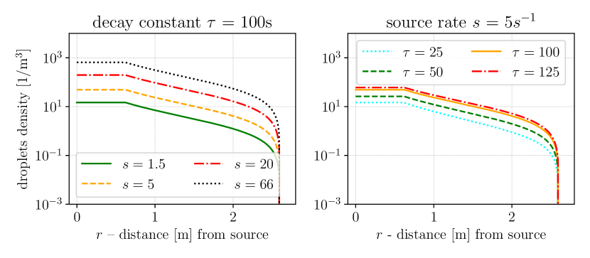
Figure 1: Swap over parameters for droplet density in the proximity of an infected individual (the source $s$ in s^-1). We use decay constant $\tau=100$s and various source rates (in the range of $1.5$ - $66$ $s^{-1}$) in the left panel, and source rate $s=5$s^-1 with various $\tau$ parameters in the range of $25$ - $125$ $s$ in the right panel.

In the final part of this subsection, recall that the parameter’s $D$ value, which reflects the diffusion and convection of the air, is rather heuristics. Its particular value in our model is based on the heuristics choice made in [5]. However, if $D$ is in some reasonable range, our model is rather not sensitive to its particular value, see Fig. 2. (From Eqs. (5) (6) can deduce that changes in $D$ may be roughly counterbalanced by changes in constant $C$.)

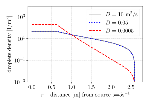
Figure 2: Sensitivity analysis of droplets density near the source $s=5$s^-1 for various diffusion constant $D$ values in Eq. (1), given decay constant $\tau=100$s. Observe similar behavior for the wide range of $D$ values.

2.2 Indirect – contaminated environmental air

To model pathogens’ spread in the compartment, but far from the source, we refer to the indirect spreading via indoor air [8]. The general dynamic of such is complex and depends on the topology in the compartment. The pathogen’s transmission at longer distances relies on small droplets and aerosol [12], while pathogens’ spread near the source more relies on large droplets. As this transition is expected not to be dominant, we apply the mean approximation. In detail, we assume that droplets (or aerosol units) contaminating environmental air are distributed uniformly over the compartment.

Assuming, that there are $S^{\prime}\in\{s_{1},s_{2},\ldots\}$ sources in the compartment of volume $V$, and following [5] (or using discussion analogical to Eq. (6)), we can compute the stationary state of the density of droplets (or aerosol units) in the compartment, namely:

$$c_{\text{b}}(s_{1},\ldots)=\frac{\tau^{\prime}\sum_{s\in S^{\prime}}s}{V}\ \ \text{droplets}/\text{m}^{3}.$$ (8)

We recognize, that transmission discussed in this subsection is relevant when mediated by small droplets (or aerosol elements) that can remain suspended in the air longer. Here decay constant denoted by $\tau^{\prime}$ is different (and higher in general) than $\tau$ in Eq. (5), for a direct way, as in indirect transmission aerosols play a more dominant role. Particular determination of $\tau^{\prime}$ must be performed with caution, best by validation with simulations.

In Fig 3 we present the density of droplets given particular ranges of values of parameters for indirect transmission via environmental air. In this particular parameters ranges, densities are considerably lower than these resulting form direct transmission in Fig. 1.

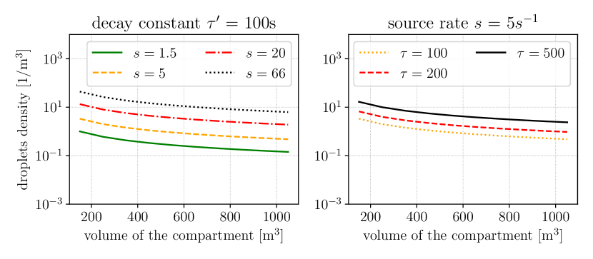
Figure 3: Swap over parameters for a density of droplets in contaminated environmental air, with one infected individual of source rate $s$.

2.3 Indirect – contaminated surface

We expect that, for factory workers, contact with contaminated workplaces or tools can also be the source of infection. Surfaces are usually contaminated by the sedimentation of droplets exhausted by an infected individual or from generally contaminated air. Here, we will however concentrate of the contamination by individual, as this way is expected to be more sound. This coincides with the modellin in [5] (and Fig. 2.1D therein), where droplets of diameter $80\mu$m or grater can sediment before evaporation. Henceforth, for surface contamination’s sake, we are interested in large droplets only. From [21] (Tab. $1$ and Fig. $3$ therein) one can conclude, that in exhausted air, there are rough $w=10\%$ of large droplets of above-mentioned size (i.e. greater or equal to $80\mu$m).

Following argumentation in Section 2.2, as the accurate model of droplet sedimentation is complex, we propose the approximation of the uniform surface contamination. Given such approximation, the source rate, i.e. the number of droplets sedimented on a unit area, in unit time is:

$$S_{s}=\frac{ws}{A}.$$ (9)

Here $A$ is the area of the surface that is being contaminated. The density of droplets on the surface (per unit area) can be modeled in time by the decay equation:

$$\frac{\partial c_{s}(t)}{\partial t}=S_{s}-\frac{c_{s}(t)}{\tau_{s}},$$ (10)

where $\tau_{s}$ is the decay constant on the surface, which differs largely from the decay constant in the air, as droplets can evaporate, be removed by ventilation, etc. To illustrate this on an example, in [22] following half-life times $T_{s,1/2}=\tau_{s}\ln(2)$ of COVID-19 virus on the surface was recorded: $5$ hours on stainless-steel surface and $7$ hours on plastic surface (these are materials often found in industry). Importantly, above mentioned time scales, are of the same order of magnitude as the length of the working shift. Hence, for surface contamination by pathogens similar to COVID-19, we can omit the decay factor in Eq. (10), yielding:

$$c_{s}(s)=\frac{ws}{A}t,$$ (11)

where $t$ is the time of the droplet’s sedimentation process. As the possible decay mechanism, we can consider disinfection. The disinfection of the surface will decrease $c_{s}$ by some percentages factor, see [23] and in particular Tab. III therein.

3 Probability of infection

As our research is dedicated to airborne pathogens, we identify spreading of droplets (or elements of the aerosol considered here as very small droplets) with pathogen spreading. Then infection can take place either by inhalation of infected droplets (spread in direct or indirect way) or be contact with a surfaced contaminated by already sedimented droplets (also indirect way).

3.1 Inhalation of droplets

In this subsection, we compute the probability of infection via droplet inhalation, no matter what mechanism of droplet spreading is considered (direct from the proximity of an infected individual or indirect from contaminated environmental air). For our model, we denote by $c$ the density of droplets in the unit volume given by Eq. (7) (in the case of direct droplet source from proximity of infected individual), or by Eq. (8) (in the case of indirect droplets source from contaminated environmental air). The number of inhaled droplets in time $t$ (assuming constant $c$) is:

$$N(t)=Qct,$$ (12)

where the breathing rate $Q$ is the model parameter. This value is tied to attributes of particular individuals, (e.g. physical effort, performed job, etc.). To account for the particular value of $Q$, let us refer to [5] where $Q$ was modeled by the probabilistic model of uniform distribution in the range $8-30$dm${}^{3}/$min, or by its mean value of $19$dm³/min. We will follow the latter approach, for probability computation in this section, however the model is easily convertible to the probabilistic approach. Bear in mind, that the value $19$dm³/min may seem to be large, especially when compared with medical measures (e.g. respiratory machine). However, we believe this value is more suitable for factory workers with physical effort, as performing various tasks.

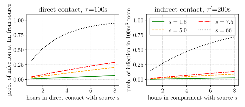
Figure 4: Probability of infection from droplets spread in a direct way from proximity of an infected individual (left panel), or in indirect way from contaminated environmental air (right panel). We assume various source rates $s$ (from $1.5$s^-1 to $66$s^-1 ). We assume $N_{b}=100$ in Eq. (13) in all cases. In left panel, we use compartment volume $V=100$m³ - for much larger industrial hale, the probability of infection in an indirect way may be negligible.

To compute the probability of infection from inhalation, one needs to determine the number of droplets $N_{b}$ exhausted by the infected individual and then inhaled by the healthy one, that will result in the latter getting infected with some threshold probability, e.g. $a=10\%$. Unfortunately, $N_{b}$ is not the universal parameter, given pathogen type, state of infection, immunity, etc. Referring to research on COVID-19 from $2020$ [5] significant level of individuals get infected if they inhale $10\leq N_{b}\leq 1000$ droplets exhausted by an infected individual. Referring to Tab $3$ in [5], and some data in [24], one can conclude that, on average, inhalation of $N_{b}=100$ droplets gives roughly $a=10\%$ the probability of getting infected. Given the above, the probability of getting infected after $t$ long inhalation can be modeled by:

$$p_{d}(t)=1-(1-a)^{\frac{N(t)}{N_{b}}},$$ (13)

where $N(t)$ is the number of droplets inhaled in time $t$. Remark that by Eq. (12) $N$ is the function of $Q$ and parameters of $c$ from Eq. (7) or Eq. (8), e.g. the source rate. We admit, that such an approach is an approximation, as it does not take into account the droplet’s size where droplets of various sizes propagate on various distances. However, the detailed approach would require much more computationally expensive simulations, deteriorating the simplicity of the model.

Computed in this way infection probabilities are presented in Fig 4 (direct way from proximity of infected individual – left panel, indirect way from contaminated environmental air – right panel). From this, we can conclude that the probability of getting infected in the indirect way (droplets from the background) even for a rather small industrial comportment of the volume of $250$m³, is relatively small, especially if the source rate can be mitigated. For a larger industrial compartment of the volume of several $1000$m³ this will be negligible. Hence, we will not analyze indirect way from contaminated environmental air further in agent-based simulations. The sensitivity analysis for various $N_{b}$ is presented in Fig. 5. Here $N_{b}=100$ is the basic scenario $N_{b}=33$ - reflects an agent with low immunity or highly infectious pathogen, and $N_{b}=300$ reflects someone with higher immunity (e.g. vaccinated). The conclusion is that long contact of an agent with low immunity with an agent with a high source rate (e.g. coughing) leads to almost certain infections. This is a rather straightforward observation that validates our model.

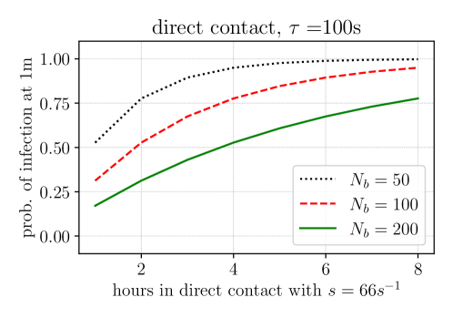
Figure 5: Probability of infection from direct contact with coughing infected individual ($s=66$s^-1), for various immunity factors $N_{b}$ in Eq. (13). Namely: $N_{b}=50$ - low immunity, $N_{b}=100$ - normal immunity, $N_{b}=200$ - high immunity (e.g. vaccinated). We assume $\tau=100$.

3.2 Infection by contact with a contaminated surface

Finally, we need to consider the indirect way of getting infected via contaminated surface. Such a way is the component of the transmission of the pathogen via the environment responsible for roughly $10\%$ of infections [13] of COVID-19. As we have not found a dedicated model for computing the probability of infection via contaminated surface, we propose the following simple model. Let $c_{s}$ be the number of droplets exhausted by the infected individual, and absorbed into the unit area surface. If enough droplets are absorbed by the surface, it can be treated as contaminated. In  [25] one genome copy (gc) /cm² was treated as a threshold of contamination of the surface. If the surface is contaminated, following  [25] the probability of a healthy individual getting infected is approx $1:10000$ for each hand-to-fomite and hand-to-facial mucosal membrane (mouth, eyes, and nose) contact.

To elaborate the model parameter with COVID-19 we are following [26], where the mean viral load is assumed to be $\text{vir}_{\text{load}}=7\times 10^{6}$ gc /ml$=7\times 10^{12}$ gc / m³ of saliva. Droplet’s diameters as discussed in [5] Fig. 2.1D are in the range of $1$-$200\mu$m; large droplets that sediments are of diameter of $80$-$200\mu$m  [21] (Tab. $1$ and Fig. $3$ therein). As discussed before in Section 2.3, we assume the rate of large droplets to all droplets to be $w=10\%$. Then we use the rough approximation of the mean diameter of a large droplet as $140\mu$m. Hence, the mean volume of large droplets is $\text{vol}_{d}=1.44\times 10^{-12}\ m^{3}$. The mean number of viral genomes in such a large droplet is

$$\nu\approx\text{vir}_{\text{load}}\text{vol}_{d}\approx 10\text{gc / droplet}$$ (14)

. Referring to Eq. (11), where $A$ is the area on which large droplets sediments, viral density after source $s$ exhausting droplets by time $t$, would be:

$$gc=c_{s}(w,s,A,t)\nu=\frac{wst}{A}\nu.$$ (15)

The time threshold of droplet sedimentation compatible with exceeding viral density of the surface equal to $gc_{\text{thres}}=1$ gc /cm${}^{2}=10000$ gc /m² (after which the surface is considered as contaminated) is:

$$t_{\text{thres}}=\frac{A\cdot gc_{\text{thres}}}{ws\nu}.$$ (16)

This threshold time is, however, highly dependent on the size of the working place, see the following examples:

• for $A=2.25m^{2}$ and $s=66$ we have $t_{\text{thres}}\approx 6$min

• for $A=2.25m^{2}$ and $s=5$ we have $t_{\text{thres}}\approx 75$min

• for $A=1m^{2}$ and $s=66$ we have $t_{\text{thres}}\approx 2.5$min

• for $A=1m^{2}$ and $s=5$ we have $t_{\text{thres}}\approx 33$min

The conclusion arises, that for small $s$ the threshold time $t_{\text{thres}}$ is rather large, here frequent disinfection of the surface (e.g. $1$ per hour) can mitigate the probability of getting infected in an indirect way from contact with a contaminated surface during the working shift. As the threshold time $t_{\text{thres}}$ value varies a lot between scenarios, we will perform simulations with the variable surface contamination probability.

As mentioned before, if the surface is contaminated, we assume that for each hand-to-fomite and hand-to-facial mucosal membrane (mouth, eyes, and nose) probability of infection from contact equals to $p_{\text{contact}}=10^{-4}$ [25]. If such contact occurs with frequency $f_{\text{contact}}$, the probability of infection is given by:

$$p(t,t_{1})=\begin{cases}tf_{\text{contact}}p_{\text{contact}}&\text{ if }t_{1}>t_{\text{thres}}\text{ Eq.~{}\eqref{eq::tthres}}\\ 0&\text{ otherwise}\end{cases}$$ (17)

where $t_{1}$ is the time spent by an infected agent at the particular surface or device prior and $t$ is the time spent by the healthy agent that can get infected. Here, no disinfection is assumed between agents’ presence at the localization.

Infection probability, assuming one hand-to-fomite and hand-to-facial mucosal membrane contact per minute, i.e. $f_{\text{contact}}=1$ min^-1 are presented in Fig. 6. These are compared to similar scenarios but from direct way from proximity of infected individual. Although in most cases infection via direct way is much more probable, the possibility of infection in mentioned here indirect way cannot be neglected, even in large volume industrial hale. This is why such indirect channels will be analyzed in agent-based simulations, provided in Section 5.

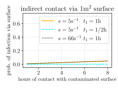
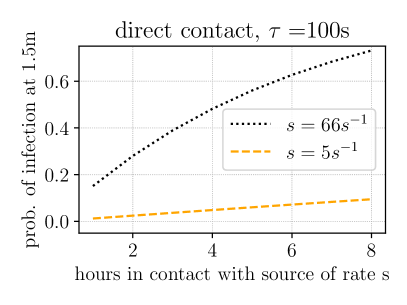
Figure 6: Probability of infection in indirect way from contact with a contaminated surface (left panel) compared with the probability of infection in direct way from proximity of infected individual (right panel). In the left panel, we use various surface contamination scenarios, namely before the contact the infected agent of source $s$ stays $t_{1}$ hours at the surface, we use $p_{\text{contact}}=10^{-4}$ [25] for modeling.

4 Simulation of droplets spreading – validation

The analytical model presented in Subsection 2.1 is simple and easy to compute. However, it contains many assumptions and simplifications concerning droplet spreading. (For validation, we have chosen the direct droplets spreading in the proximity of the source, as such way is the most important one in the disease spreading mechanism.) Hence, we aim to validate it through droplet dynamics simulations. Bear in mind however that such simulations are expensive in terms of computational time, presented here results are from the simulation that took 9-10 days on the GPU depending on the simulation parameters.

We have performed simulations of droplet dynamics in a $5\times 5\times 2.5m^{3}$ room in the following way. We used the Lattice Boltzmann method [27] implemented with the lbmpy Python module to simulate the motion of labeled air particles, with the usually used parameters: kinematic viscosity $1.516\times 10^{-5}m^{2}/s$, maximum physical velocity is 1 m/s, D3Q15 equilibrium moments, the Single Relaxation Time model with relaxation rate $1.994$, and the Smagorinsky turbulence model. We used a proprietary breathing model to force a change in respiratory air velocity. We used an advection-diffusion approach to simulate the movement of droplet particles concerning marked air particles, we used the following parameters: diffusion coefficient of $23.9\times 10^{-6}m^{2}/s$, Q27 diffusion direction pattern. The droplet particles are initially found only in the lungs of the infected person. As opposed to large droplets that sediments, see Section 2.3, we use here small droplets approximation and no droplets decay (the decay mechanism is mimicked by using limited simulation time). Here we follow simulation methodology in [28] then we consider small droplets’ sizes with the mean diameter of $1\mu$m. This is consistent with the mass-less approximation, see Section $7.3$ in [5] (as we simulate particles of diameter up to $10\mu$m). From simulations, we achieve unit-less droplets density that is then recalculated to droplets/m³, to be compatible with results in Section 2. It is worth mentioning that our simulations do not consider any air movement caused by factors other than breathing. This may cause the observation, that in real scenarios, the droplet spread is a bit larger than from ideal conditions in simulations.

We have performed two simulation settings, namely: emit and absorb. Every simulation takes in total of 20 minutes, and data are collected continuously with some time step. The emit setting concerns the spread of droplets’ density in the proximity of the infected individual, hence it can be applied to assess the analytical model of droplets’ density in proximity via Eq. (7). The second absorb setting concerns the absorption of droplets/aerosols from the air by a healthy individual. The density of droplets in the air was given from the emit simulation (after the whole cycle of $20$ minutes) assuming various distances of the infected individual ($r$). Hence it can be modeled to assess the overall mechanism of getting infected in the compartment parameterized by the particular location of the infection source.

The assessment of the analytical model with simulations in emit setting (after the whole simulation cycle of 20 minutes) is presented in Fig. 7. Concerning simulations, distance on the $y$-axis in the 1$D$ slide of $3$D spatial locations in the mouth direction (droplet’s density in other directions are similar for validity region). Finally, we did not model droplet decay (e.g. evaporation, sedimentation) in simulations; to overcome this problem we took the simulation time of the order of magnitude of the decay constant discussed Section 2 and [5]. Namely, we use simulation time in the range of $100$s - $300$s, a shorter simulation time is expected to model a non-stationary state, while a longer simulation time is far beyond the decay half-life in the proximity of the source.

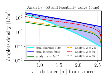
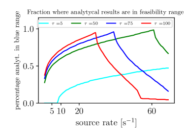
Figure 7: Emit setting, assessment of the analytical model of droplets in proximity (Eq. (7)) by the feasibility range computed from simulations - the blue area (left panel) computed for simulation time between $100$s and $300$s (the range on $x$-axis limited by $r_{0}=0.62$ and $d_{\max}=2.6$). Assessment of particular $\tau$ constant (right panel), where the percentage of analytical result in the feasibility range from simulations is depicted; observe, that $\tau=50$s models well high source rate, what is important in our model.

The analytical model returns outputs that fit into the range returned by simulations, especially for distances higher than $1.5$m for lower source intensity, this is the sound result as workers usually do not work face-to-face contact. Referring to the right panel of Fig. 7 the fair agreement between simulations and analytical model, for the range of source intensities $s$, is reached for $\tau=50$s, this value is still reasonable as we refer to [5]. From simulations, we also conclude, that low values of the source rate ($s$) do not fit simulations. To overcome this, at least partially, we suggest raising the source rate value for speaking individual from $s=5$ s^-1 suggested in Section 2 to $s=7.5$ s^-1. We recognize that in the analytical model, we used Eq. (7), i.e. we only considered the direct infection from the individual (direct way). As during simulations, the individual is placed in the compartment of a given volume ($62.5$ m³ in particular) more sound analysis should also consider the indirect way via contaminated environmental air. This (indirect way) will be considered in the next simulation setting discussed in the following paragraph.

In Fig 8 we compute the probability of a healthy individual getting infected from the proximity of the source and and infected air using the analytical model and simulations in absorb setting. Here, in analytical model we use source value $s=7.5$ s^-1 and the range of $\tau^{\prime}$, considerably larger than $\tau$ determined in Fig 7. Concerning the proximity of the infected individual, we analyze distances higher or equal to $1.5$m, which are in the validity range from Fig. 7. Given these distances, in analytical model we include the effect of an indirect way of infection via contaminated air in the compartment. Hence, the probability of infection from droplets spread from proximity and environmental air is considered in the analytical model.

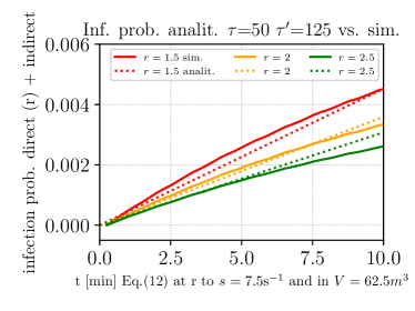
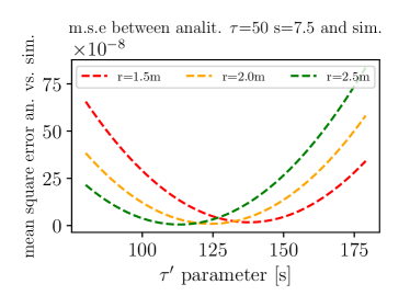
Figure 8: Absorb setting. In the left panel probability of infection computed from the analytical model and simulations is depicted as the function of time the agent inhales invective droplets/aerosol ($t$ [min]). In the right panel, the mean square error between the analytical model and simulations for various values of $\tau^{\prime}$ parameter is depicted. For both analytical model and simulations probability of infection is computed via. Eq. (13), with immunity factor $N_{b}=100$ from a number of inhaled droplets computed via simulations (solid) and analytical model (dashed). In the analytical model number of inhaled droplets computed from Eq. (12) via droplet’s density from proximity (direct) in Eq. (7) and environmental air (indirect) in Eq. (8). From the right panel, the reasonable range of $\tau^{\prime}$ parameter is $100-150$s, and the midpoint of $\tau^{\prime}=125$ can be selected as the sound value of this parameter.

From Fig. 7 we can conclude that the infection probability computed from the analytical model and simulations of inhaled droplets are similar. Here, we use various values of time ($t$) of the individual inhaling the contaminated air. This time is assumed to be meaningfully shorter than the duration of the emission stage, hence we reduce possible effects tied to the temporal separation of emission and absorption. The meaningful result of the comparison yields $\tau^{\prime}$ parameter (of indirect infection spread via environmental air in Eq. (8)) to be in the range $100-150$s, namely higher than the proposed $\tau$ value of infection via direct contact.

Finally, the impact of various masks from simulations in emit setting is presented in Fig. 9 in the form of the fraction of droplets reduced by the mask, i.e. $\frac{c_{\text{no mask}}-c_{\text{mask}}}{c_{\text{no mask}}}$. Although this value is distance-dependent and mask-dependent, we can model the good mask by reducing the source $s$ by $40\%$ as in [20]. The ordinary mask would reduce the source rather by a value closer to $20\%$.

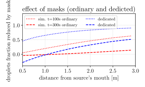
Figure 9: Simulation results of the reduction of droplets density due to application of various masks, compare the effect of the ordinary mask, and dedicated mask. Simulation times higher than $300$s would be much higher than the decay constant from Section 2.

5 Agent-based simulations

To place our previous findings closer to the industrial reality, and demonstrate that a simple random walk model can mimic the pathogen’s spreading, we analyze the spread of disease in the simple simulated environment. Besides, the goal of the presented simulations is to get insight into the relative strength of two ways of infection spreading, direct and indirect, under variable parameters of the model. Using agent-based simulations, we compare the impact of the most probable direct way of infection from proximity to an infected individual with indirect way of infection from contact with a contaminated surface.

We expect that the agents’ density, rather than the actual size of an industrial facility, is the most important factor in deciding about the infection spread. Nevertheless, for large industrial facility, the contaminated environment air infection probability may be rather negligible, but the contact of workers with potentially contaminated tools and machines cannot be neglected.

In this section, we use an agent-based model, developed to mimic the movement of individuals in an environment resembling the industrial workplace. To model the industrial environment, we use rectangle areas with spatial resolution $r=1.5$ m. The simulation step corresponds to $\delta t=60$ s = $1$ min of real-time. Hence, the $8$h working shift will correspond to $480$ simulation steps.

As in many infections such as COVID-19, in particular, the infected agent is not infecting immediately, we use the latency factor, namely the period in which the infected individual is not infecting others. In this particular experiment, we set the latency period parameter to be one day. Hence, for the results presented in this section, newly infected individuals do not infect others.

Figure 10: User interface of the NetLogo model used in this paper. The screen presents an example of one run of the simulation cycle corresponding to one day. Black elements represent walls, blue elements represent machines or workplaces. The source code of this mode can be obtained from [29].

The elements of the simulated object mimic compartments, machines, or workplaces, and the passing between compartments, see Fig. 10. Through this, agents move randomly, with the mobility parameter $\mu$, defined as the probability of altering the position during each simulation step. To mimic working at a given workplace, the process of slowing down the random movement of agents near particular locations is implemented. Technically, it is performed by modifying the mobility factor $\mu$, by $10^{-2}$ close to locations that mimic workplaces. The model used in this section was implemented using NetLogo multi-agent programmable modeling environment [30].

At the starting point of the simulation, we pick a given number of infected agents. The infected agent can infect others directly by contact or indirectly by contaminating the surface (patch) that simulates the workplace. As the development of the disease process is assumed to be much longer than the working shift, we assume that contaminated patches and infected agents do not heal during the working shift. Based on these assumptions, we consider the following possible ways of infection:

1. Direct contact with an infected individual. Taking the spatial resolution of our simulation, we consider potential infection if two agents are at the same pixel, distanced by $r=0.75$ m, or neighbor pixels distanced by $r=1.5$ m. The probability of getting infected during a $\delta t$ step is approximated from Eq. (13) by:

   $$\delta p_{\text{direct}}\approx a\frac{N(\delta t)}{N_{b}},$$ (18)

   for small $\delta t$. Then using Eq. (12) and Eq. (7) we have:

   $$\delta p_{\text{direct}}=a\frac{Q\hat{c}(r,s)}{N_{b}}\delta t.$$ (19)

   Taking $Q=19$dm³/min = $3.16\cdot 10^{-4}$m³/s, $N_{b}=100$, $a=0.1$ and computing $\hat{c}(r,s)$ via Eq. (7) with parameters $\tau=50$s, $D=0.05$m²/s, $r_{0}=0.62$m, $d_{\max}=3.5$m, and using source rate $s=66$ s^-1 that represents the coughing individual according to discussion in Section 2 and is fairly validated by Fig. 7 left, we have:

   $$\delta p_{\text{direct}}\approx\begin{cases}0.0049$ min${}^{-1}&\text{meet at the same patch}\\ 0.0013$ min${}^{-1}&\text{meet at neighbour patches}\end{cases}$$ (20)

2. Indirect, from contact with contaminated surface. As the probability of patch getting infected is highly parameter dependent (e.g. the area of the working place), we use variable patch infection possibility, to assess for various scenarios. Hence, for simulations we assume that in each ($1$min long) step the patch can get infected with a certain probability, called the patch contamination probability that varies from $0$ to $0.5$ with some resolution step.

   

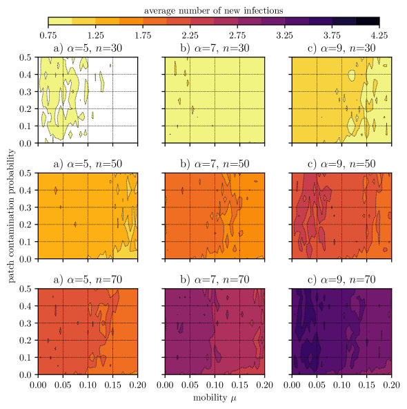
   Figure 11: Mean increase in the number of infected agents for different values of mobility parameter $\mu\in[0.0,0.5]$, different populations, $n=30,50$ and $70$ agents, and different number of initially infected agents, $\alpha=5,9$ and $9$. Each plot represents the absolute increase in the number of agents infected during one day in the population $\alpha$ of initially infected agents, with different values of probability contaminating the items, and with different mobility $\mu$ of the agents. We use the source rate of $s=66$ s^-1 (see: Eq. 20). Mean is calculated over $10^{4}$ realizations. No healing process is considered.

   To compute the probability of an agent getting infected from the surface, we use Eq. (17) with $p_{\text{contact}}=10^{-4}$ and $f_{\text{contact}}=1$ min^-1):

   $$\delta p_{\text{undir. c}}\approx 0.0001\text{ min}^{-1}.$$ (21)

Simulation results in numbers of newly infected agents are presented in Fig. 11. The density of agents is changed between $n=30,50$ and $70$.

The straightforward conclusion is that concentrations of agents favor infection spreading. Hence, limiting the number of people working at the same time on premises should be used as the first line of defense from infection spread. However, one can also conclude that in the presented case, although the increase in mobility leads to the decreased number of new infections, there appears local maxim in infection at a mobility factor of $\mu\approx 0.05$. This indicates the sound finding, that there is a certain mobility level at which infection is most probable.

Figure 12: Dependency between the number of infected agents and the agents’ mobility $\mu$. Each row represents a series of histograms for different numbers of initially infected agents, while each column a series of histograms for different agents’ mobility factor $\mu$. Histograms represent the occurrences (counts) of the number of new infections, for a fixed number of initially infected agents, for the case $n=30$ (red solid line) and the case $n=70$ (blue dashed line). Patch contamination probability is set to $0.5$. Histograms are calculated over $10^{4}$ realizations.

Another aspect we are interested in is the impact of an agent’s mobility and population density on the propagation of infection. The results illustrating detailed analysis of this impact are presented in Fig. 12. First, it can be seen in the top row of Fig. 12 that for a small number of initially infected agents mobility does not play a significant role in the infection propagation, and this effect is observed for small and large populations. For the case where the initial number of infected agents amounts to approximately 7%-15% of the population (middle row of Fig .12, case with $\alpha=5$), the increase in the mobility can lead to the decrease in the new cases for both large and small population density. However, for the larger number of initially infected agents, the density of all agents is crucial for the dynamics of the infection. In this case, as one can see in the bottom row of Fig .12, the larger density of individuals ensures a larger increase in the number of new infections. On the other hand, the smaller population of $n=30$ agents – and hence the smaller density of individuals – leads to a decrease in new infection with the increase in mobility. This effect does not occur for the larger population of $n=70$ agents. This suggests that for larger populations the mobility of agents is not crucial for the stable increase in the number of cases.

6 Conclusions

Nowadays, after the severe outbreaks of the COVID-19 pandemic, there is a growing understanding that outbreaks of dangerous pathogens are possible. Based on this experience, we understand that society has to prepare for another outbreak of an epidemic (not necessarily COVID-19) in such a way that the economy and supply chain will not be disturbed too much. For the strategic planning of industrial work in times of such an epidemic, one can take advantage of the following conclusions of our research.

We have introduced a new analytical model of pathogen spreading that is computationally inexpensive, making it a potentially preferable alternative to more computationally intensive simulations in some situations. We recognize, however, that the model relies on several simplifying assumptions and a wide range of parameters. The general conclusion is that the analytical model can reproduce simulations in many cases, while proper parameter tuning can be performed when comparing the analytical model with simulations. In this simple example, we demonstrate how simulations can be applied to validate analytical model and show that simulations can be meaningful tools to determine the parameters’ validity ranges. Henceforth, in practical application, simulations can be run only once to validate the analytical model, and then the latter can be used on the day-to-day basis to ensure safety in the industry. From the validation point of view, we, for example, recognize, that our analytical model, has limitations, while modeling the infection spread close to the source, see Fig. 7.

To validate the analytical model from another perspective, let us acknowledge that from the analytical model general countermeasures can be drawn, these are: removal of coughing/ sneezing workers from the common workplace, or immediately imposing high-quality masks on such individuals, then reducing agent density, then reducing agent’s mobility (or imposing mandatory high-quality masks on highly mobile workers), disinfection of surfaces. So, countermeasures should concern the direct channel of infection first. Countermeasures that focus mainly on the indirect channels, such as disinfection of surfaces, can be imposed in succession.

Finally, the role of agent-based simulations was demonstrative. We recognize that it would be valuable if the authors applied the simulation to a real-world industrial topology with realistic movements within the plant, perhaps based on actual measurements. Although the direct industrial data we have is confidential, further more detailed research shall enhance the relevance and applicability of the agent-based model, which currently remains a largely theoretical exercise. Nevertheless, we draw an unexpected conclusion, that there is a certain level of mobility of agents, where the infection is most probable. This conclusion needs further investigation.

Data availability

Source code used for simulating the model discussed in this work and sample simulation results can be obtained from [29].

Declaration of competing interest

The authors declare that they have no known competing financial interests or personal relationships that could have appeared to influence the work reported in this paper. All authors reviewed the manuscript.

References

- [1] B. R. Rowe, A. Canosa, J.-M. Drouffe, J. Mitchell, Simple quantitative assessment of the outdoor versus indoor airborne transmission of viruses and COVID-19, Environmental research 198 (2021) 111189. doi:10.1016/j.envres.2021.111189.
- [2] W. R. Milligan, Z. L. Fuller, I. Agarwal, M. B. Eisen, M. Przeworski, G. Sella, Impact of essential workers in the context of social distancing for epidemic control, PLoS One 16 (8) (2021) e0255680. doi:10.1371/journal.pone.0255680.
- [3] T. Chen, Y.-C. Wang, M.-C. Chiu, Assessing the robustness of a factory amid the COVID-19 pandemic: A fuzzy collaborative intelligence approach, in: Healthcare, no. 4 in 8, 2020, p. 481. doi:10.3390/healthcare8040481.
- [4] X. Li, B. Wang, C. Liu, T. Freiheit, B. I. Epureanu, Intelligent manufacturing systems in COVID-19 pandemic and beyond: framework and impact assessment, Chinese Journal of Mechanical Engineering 33 (1) (2020) 1–5. doi:10.1186/s10033-020-00476-w.
- [5] V. Vuorinen, M. Aarnio, M. Alava, V. Alopaeus, N. Atanasova, M. Auvinen, N. Balasubramanian, H. Bordbar, P. Erästö, R. Grande, N. Hayward, A. Hellsten, S. Hostikka, J. Hokkanen, O. Kaario, A. Karvinen, I. Kivistö, M. Korhonen, R. Kosonen, J. Kuusela, S. Lestinen, E. Laurila, H. J. Nieminen, P. Peltonen, J. Pokki, A. Puisto, P. Råback, H. Salmenjoki, T. Sironen, M. Österberg, Modelling aerosol transport and virus exposure with numerical simulations in relation to SARS-CoV-2 transmission by inhalation indoors, Safety Science 130 (2020) 104866. doi:10.1016/j.ssci.2020.104866.
- [6] B. M. Castro, Y. d. A. de Melo, N. F. Dos Santos, A. L. da Costa Barcellos, R. Choren, R. M. Salles, Multi-agent simulation model for the evaluation of COVID-19 transmission, Computers in Biology and Medicine 136 (2021) 104645. doi:10.1016/j.compbiomed.2021.104645.
- [7] R. Karia, I. Gupta, H. Khandait, A. Yadav, A. Yadav, COVID-19 and its modes of transmission, SN Comprehensive Clinical Medicine (2020) 1–4doi:10.1007/s42399-020-00498-4.
- [8] J. Cai, W. Sun, J. Huang, M. Gamber, J. Wu, G. He, Indirect virus transmission in cluster of COVID-19 cases, wenzhou, china, 2020, Emerging Infectious Diseases 26 (6) (2020) 1343. doi:10.3201/eid2606.200412.
- [9] A. Fadaei, Ventilation systems and COVID-19 spread: evidence from a systematic review study, European Journal of Sustainable Development Research 5 (2) (2021) em0157. doi:10.21601/ejosdr/10845.
- [10] L. Bourouiba, Turbulent gas clouds and respiratory pathogen emissions: potential implications for reducing transmission of COVID-19, Journal of the American Medical Association 323 (18) (2020) 1837–1838. doi:10.1001/jama.2020.4756.
- [11] L. Morawska, J. Cao, Airborne transmission of SARS-CoV-2: The world should face the reality, Environment International 139 (2020) 105730. doi:10.1016/j.envint.2020.105730.
- [12] M. Meselson, Droplets and aerosols in the transmission of sars-cov-2, New England Journal of Medicine 382 (21) (2020) 2063–2063. doi:10.1056/NEJMc2009324.
- [13] L. Ferretti, C. Wymant, M. Kendall, L. Zhao, A. Nurtay, L. Abeler-Dörner, M. Parker, D. Bonsall, C. Fraser, Quantifying SARS-CoV-2 transmission suggests epidemic control with digital contact tracing, Science 368 (6491) (2020). doi:10.1126/science.abb6936.
- [14] T. Greenhalgh, J. L. Jimenez, K. A. Prather, Z. Tufekci, D. Fisman, R. Schooley, Ten scientific reasons in support of airborne transmission of sars-cov-2, The lancet 397 (10285) (2021) 1603–1605.
- [15] D. Duval, J. C. Palmer, I. Tudge, N. Pearce-Smith, E. O’connell, A. Bennett, R. Clark, Long distance airborne transmission of sars-cov-2: rapid systematic review, bmj 377 (2022).
- [16] K. Domino, J. A. Miszczak, Will you infect me with your opinion?, Physica A: Statistical Mechanics and its Applications 608 (2022) 128289. doi:10.1016/j.physa.2022.128289.
- [17] J. Wei, Y. Li, Airborne spread of infectious agents in the indoor environment, American journal of infection control 44 (9) (2016) S102–S108. doi:10.1016/j.ajic.2016.06.003.
- [18] J. Wei, Y. Li, Enhanced spread of expiratory droplets by turbulence in a cough jet, Building and Environment 93 (2015) 86–96. doi:10.1016/j.buildenv.2015.06.018.
- [19] S. Asadi, A. S. Wexler, C. D. Cappa, S. Barreda, N. M. Bouvier, W. D. Ristenpart, Aerosol emission and superemission during human speech increase with voice loudness, Scientific Reports 9 (1) (2019) 1–10. doi:10.1038/s41598-019-38808-z.
- [20] N. H. Leung, D. K. Chu, E. Y. Shiu, K.-H. Chan, J. J. McDevitt, B. J. Hau, H.-L. Yen, Y. Li, D. K. Ip, J. M. Peiris, et al., Respiratory virus shedding in exhaled breath and efficacy of face masks, Nature Medicine 26 (5) (2020) 676–680. doi:10.1038/s41591-020-0843-2.
- [21] C. Y. H. Chao, M. P. Wan, L. Morawska, G. R. Johnson, Z. Ristovski, M. Hargreaves, K. Mengersen, S. Corbett, Y. Li, X. Xie, et al., Characterization of expiration air jets and droplet size distributions immediately at the mouth opening, Journal of Aerosol Science 40 (2) (2009) 122–133. doi:10.1016/j.jaerosci.2008.10.003.
- [22] N. van Doremalen, T. Bushmaker, D. H. Morris, M. G. Holbrook, A. Gamble, B. N. Williamson, A. Tamin, J. L. Harcourt, N. J. Thornburg, S. I. Gerber, et al., Aerosol and surface stability of hcov-19 (sars-cov-2) compared to sars-cov-1, MedRxiv (2020). doi:10.1101/2020.03.09.20033217.
- [23] G. Kampf, D. Todt, S. Pfaender, E. Steinmann, Persistence of coronaviruses on inanimate surfaces and their inactivation with biocidal agents, Journal of Hospital Infection 104 (3) (2020) 246–251. doi:10.1016/j.jhin.2020.01.022.
- [24] J. Lu, J. Gu, K. Li, C. Xu, W. Su, Z. Lai, D. Zhou, C. Yu, B. Xu, Z. Yang, COVID-19 outbreak associated with air conditioning in restaurant, guangzhou, china, 2020, Emerging Infectious Diseases 26 (7) (2020) 1628. doi:10.3201/eid2607.200764.
- [25] A. M. Wilson, M. H. Weir, S. F. Bloomfield, E. A. Scott, K. A. Reynolds, Modeling COVID-19 infection risks for a single hand-to-fomite scenario and potential risk reductions offered by surface disinfection, American Journal of Infection Control 49 (6) (2021) 846–848. doi:10.1016/j.ajic.2020.11.013.
- [26] R. Wölfel, V. M. Corman, W. Guggemos, M. Seilmaier, S. Zange, M. A. Müller, D. Niemeyer, T. C. Jones, P. Vollmar, C. Rothe, et al., Virological assessment of hospitalized patients with COVID-2019, Nature 581 (7809) (2020) 465–469. doi:10.1038/s41586-020-2196-x.
- [27] T. Krüger, H. Kusumaatmaja, A. Kuzmin, O. Shardt, G. Silva, E. M. Viggen, The lattice boltzmann method, Springer International Publishing 10 (978-3) (2017) 4–15. doi:10.1007/978-3-319-44649-3.
- [28] A. G. Antonis P. Papadakis, Aimilios Ioannou, W. Almady, Kyamos software – cloud gpu infiniband tool for modeling covid19, Journal of Multidisciplinary Engineering Science and Technology 8 (10) (2021) 14678–14691.
-
[29]
J. A. Miszczak, K. Domino, A. Sochan,
Agent-based
simulation for the validation of indoors virus propagation model (2024).
URL https://github.com/jmiszczak/indoors_virus_propagation_model -
[30]
U. Wilensky, Netlogo multi-agent
programmable modeling environment. (1999).
URL http://ccl.northwestern.edu