The Detection and Correction of Silent Errors in Pipelined Krylov Subspace Methods

Abstract

As computational machines are becoming larger and more complex, the probability of hardware failure rises. “Silent errors”, or, bit flips, may not be immediately apparent but can cause detrimental effects to algorithm behavior. In this work, we examine an algorithm-based approach to silent error detection in the context of pipelined Krylov subspace methods, in particular, Pipe-PR-CG, for the solution of linear systems. Our approach is based on using finite precision error analysis to bound the differences between quantities which should be equal in exact arithmetic. Through inexpensive monitoring during the iteration, we can detect when these bounds are violated, which indicates that a silent error has occurred. We use this approach to develop a fault-tolerance variant and also suggest a strategy for dynamically adapting the detection criteria. Our numerical experiments demonstrate the effectiveness of our approach.

1 Introduction

We consider the problem of solving the linear system $Ax=b$, where $A\in\mathbb{R}^{n\times n}$ is symmetric positive definite. We are particularly interested in the case where $A$ is very large and sparse, in which case the conjugate gradient method [13] is usually the method of choice.

In large-scale settings, the high cost of communication in HSCG motivated the search for mathematically equivalent CG variants better suited for implementation on parallel machines, as with less communication we might be able to speed up the overall computation. One possibility is to introduce auxiliary vectors and rearrange the procedure in a way that reduces the necessary number of synchronization points to only one, and “pipeline” the inner product reductions and matrix operations to occur concurrently, so that the global synchronization points no longer cause a bottleneck. This is the strategy introduced in the “pipelined CG” method of Ghysels and Vanroose [11]. However, such communication-hiding variants may amplify the numerical problems which already exist in HS-CG such as delayed convergence, or may worsen the maximal attainable accuracy (the level at which the approximation error $||\mathbf{x-x_{k}}||$ starts to stagnate) due to the sensitivity of CG to rounding errors [6].

A solution to these numerical problems was developed in [6]. Here, the authors employ the newly introduced expressions as a “predicted” value, which is then used instead of the original expression to compute the next few steps until it is “recomputed” using the original above written inner product. This so-called “predict and recompute” variant (Pipe-PR-CG) helps mitigate the deviation of true quantities and their values approximated by recurrences. This idea was based on the previous work of Meurant [16] which aimed to stabilize the HS-CG algorithm while also retaining the potential for parallelism.

As computational machines are becoming increasingly large and more complex, the probability of failure grows, and thus the topic of error handling and fault-tolerant algorithms is now more important than ever. Some errors are rather simple to detect, since they, e.g., result in a crash of the computation. However, there is another category of faults: so-called “silent errors”. These faults may not be immediately easily apparent, but they can result in significantly altered behavior of the used numerical method. There has been a significant amount of work in studying the effect and detection of silent errors in numerical linear algebra computations; see, e.g., [1, 14, 9, 3, 10, 4]. One way of detecting silent errors is to perform the computation multiple times, and compare the results. However, this substantially increases the overall computational cost, in terms of both time and energy. Therefore, it is desirable to possess an alternative, more efficient approach.

In this work, we derive effective and inexpensive methods for silent error detection in Pipe-PR-CG that can be subsequently incorporated into a modified version of the algorithm which is able to automatically detect and correct the silent faults. These detection methods are based on the comparison of “gaps” between certain quantities which are equal in exact arithmetic and the bounds on their values in finite precision. After providing relevant background in Section 2, in Section 3 we provide a set of experiments which demonstrates the sensitivity of Pipe-PR-CG to silent errors. Section 4 focuses on constructing several criteria for the detection of silent errors in the Pipe-PR-CG algorithm based on floating point rounding error analysis, and in Section 5, we present a fault-tolerant variant and experimental results demonstrating the effectiveness of the detection criteria. Based on insights from these experiments, in Section 6, we develop an adaptive version of the fault-tolerant algorithm which can dramatically reduce the number of false positive detections.

2 Background

2.1 Silent errors

A key concept of this article are so-called “silent errors”, also known as “soft faults” [14] or “silent data corruption” (SDC) [9]. Silent errors are faults that do not terminate the computation or raise an error, but rather cause a change in some floating-point number without any apparent indication of a problem [14]. Silent errors may be qualified in several ways from both the low-level point of view (what is their hardware-wise cause) and the high-level point of view (in what way they affect the logical values involved in a computation).

In this work, we assume that silent errors are transient; that is, if an input to a computation is altered by a silent error, the result of the computation will be affected, but the error will not be persistent in the input after the computation. This is common in practice, since inputs to a computation are in transient memory (cache); the same model is used, e.g., in [9] or [2].

We also assume that silent errors occur in the form of bit flips, since they are commonly studied [9] and easy to model. Note that the impact of a bit flip may vary. A bit flip in the end of the mantissa of a floating-point number may have only negligible effects, whereas a flip of some dominant bit in the exponent can destroy the entire computation. This motivates why the topic of silent errors might be potentially crucial in practice. Especially, as supercomputers are becoming more complex and the number of their parts increases, the risk of a hardware failure increases as well [14]. Moreover, the relaxation of hardware correctness could be utilized as a way to save energy [9]. Additionally, the decrease of transistor feature sizes makes individual components more prone to failure [9].

The most straightforward approaches for detecting silent errors are so-called double modular redundancy (DMR) and triple modular redundancy (TMR) [2]. These methods are based on the idea that we can perform the same computation multiple times, either consecutively on the same hardware unit or simultaneously on different hardware units, and then check whether the results are the same [2]. The crucial problem of redundancy approaches is their cost, as they require either multiple computational units or twice/thrice the time. This is especially limiting for large, massively parallel computers because of their energy consumption [9].

Another possible idea for the detection of silent errors, which we use in this article, is to use information about the numerical method to derive some detection criteria [14]. This approach is called algorithm-based fault tolerance (ABFT) [14]. Even though ABFT methods do not require the amount of computational resources needed for the redundancy approaches, they still require some. They may also cause delayed convergence if the algorithm is modified to utilize them to correct the found errors during the computation [14].

2.2 The Pipe-PR-CG algorithm

The original conjugate gradient method of Hestenes and Stiefel [13] (HS-CG) is stated in Algorithm 1. From now on, vector variables are written in bold and matrices in bold uppercase. Here, $\mathbf{M}$ denotes a symmetric positive definite “preconditioner” matrix, which is used to improve properties of the system. Using $\mathbf{M}$, we can implicitly solve the system $\mathbf{L^{-T}AL^{-1}y}=\mathbf{L^{-T}b}$, where $\mathbf{y}=\mathbf{Lx}$ and $\mathbf{L}$ is the Cholesky factor of $\mathbf{M}$, utilizing just solutions of subsystems with $\mathbf{M}$ during the run, e.g., $\mathbf{\tilde{r}_{k}}=\mathbf{M^{-1}}\mathbf{r_{k}}$ [6]. The symbol $\sim$ denotes extra variables introduced by inclusion of the preconditioner. The statement of the INITIALIZE() procedure can be found in Appendix A.

Algorithm 1 Hestenes and Stiefel Conjugate Gradient: HS-CG (preconditioned)

1:procedure HS-CG($\mathbf{A},\mathbf{M},\mathbf{b},\mathbf{x_{0}}$)

2:     INITIALIZE()

3:     for $k=1,2,\dots$ do

4:         $\mathbf{x_{k}}=\mathbf{x_{k-1}}+\alpha_{k-1}\mathbf{p_{k-1}},\quad\mathbf{r_{k}}=\mathbf{r_{k-1}}-\alpha_{k-1}\mathbf{s_{k-1}},\quad\mathbf{\tilde{r}_{k}}=\mathbf{M^{-1}}\mathbf{r_{k}}$

5:         $\nu_{k}=\langle\mathbf{\tilde{r}_{k}}$, $\mathbf{r_{k}}\rangle,\quad\beta_{k}=\nu_{k}/\nu_{k-1}$

6:         $\mathbf{p_{k}}=\mathbf{\tilde{r}_{k}}+\beta_{k}\mathbf{p_{k-1}}$, $\mathbf{s_{k}}=\mathbf{Ap_{k}}$

7:         $\mu_{k}=\langle\mathbf{p_{k}},\mathbf{s_{k}}\rangle,\quad\alpha_{k}=\nu_{k}/\mu_{k}$

8:     end for

9:end procedure

Taking a look at Algorithm 1, we can observe that the computation has to be done largely sequentially, since each step directly depends on variables computed in the previous ones. This causes trouble on parallel distributed memory computers, where a communication bottleneck is created because of the inability to overlap computation with expensive global reductions from inner products or with at least some amount of communication from the matrix-vector multiplication [6]. Specifically, there are two so-called global synchronization points at the inner products [5].

The high cost of communication in HS-CG motivates the search for mathematically equivalent CG variants better suited for implementation on parallel machines, as with less communication we might be able to speed up the overall computation. One possibility is to rearrange the procedure in a way that reduces the necessary number of synchronization points to only one. However, such communication-hiding variants (e.g., the variant of Chronopoulos and Gear [7]) may amplify the numerical problems which already exist in HS-CG such as delayed convergence, or may worsen the maximal attainable accuracy (the level at which the approximation error $||\mathbf{x-x_{k}}||$ starts to stagnate) due to the sensitivity of CG to rounding errors [6].

On top of that, we would like to “pipeline” the inner product reductions and matrix operations to occur concurrently, so that the global synchronization points no longer cause a bottleneck, as in the variant of Ghysels and Vanroose [11]. Nonetheless, once we try to include pipelining, the above-mentioned numerical issues can become even more grave [5, 6].

A pipelined variant which overcomes to a large extent the numerical shortcomings of previous variants is the Pipe-PR-CG method of [6], shown in Algorithm 2. Pipe-PR-CG still requires only one global synchronization point per iteration. This is done by deriving a mathematically equivalent expression for the variable $\nu_{k}$ (line 5 in Algorithm 1), utilizing quantities already computed in the previous iteration. This way we avoid the first computation of the inner product $\nu_{k}=\langle\mathbf{\tilde{r}_{k}}$, $\mathbf{r_{k}}\rangle$. However, this change could lead to a dramatic loss of accuracy as the value of $\nu_{k}$ could become negative [6], and therefore we employ the new expression just as a “predicted” value, which is then used instead of the original expression to compute the next few steps until it is “recomputed” using the original above written inner product. This idea was proposed by Meurant in [16] to stabilize the algorithm while also retaining the potential for parallelism. Although even this alteration might introduce some instability to the algorithm, it allows us to perform the iteration more efficiently on distributed memory machines as there is less need for data communication, since all the inner products occur at the same time [6]. Moreover, the maximal attainable accuracy is similar as for the original HS-CG. This perhaps somehow surprising result is thoroughly analyzed in [6]; we refer the reader to this work for a full derivation of the method.

We focus on the Pipe-PR-CG method here for two reasons. First, it is the current state-of-the-art pipelined Krylov subspace method in terms of potential for parallel performance and numerical stability. Second, the predict-and-recompute aspect of the method provides ample opportunities for developing silent error detection approaches based on finite precision bounds. In short, the “predicted” and “recomputed” variables, which should be the same in exact arithmetic, provide quantities which can be easily and inexpensively compared.

Algorithm 2 Pipelined Predict-and-Recompute Conjugate Gradient:
Pipe-PR-CG (preconditioned)

1:procedure Pipe-PR-CG($\mathbf{A},\mathbf{M},\mathbf{b},\mathbf{x_{0}}$)

2:     INITIALIZE()

3:     for $k=1,2,\dots$ do

4:         $\mathbf{x_{k}}=\mathbf{x_{k-1}}+\alpha_{k-1}\mathbf{p_{k-1}}$

5:         $\mathbf{r_{k}}=\mathbf{r_{k-1}}-\alpha_{k-1}\mathbf{s_{k-1}},\quad\mathbf{\tilde{r}_{k}}=\mathbf{\tilde{r}_{k-1}}-\alpha_{k-1}\mathbf{\tilde{s}_{k-1}}$

6:         $\mathbf{w^{\prime}_{k}}=\mathbf{w_{k-1}}-\alpha_{k-1}\mathbf{u_{k-1}},\quad\mathbf{\tilde{w}^{\prime}_{k}}=\mathbf{\tilde{w}_{k-1}}-\alpha_{k-1}\mathbf{\tilde{u}_{k-1}}$

7:         $\nu^{\prime}_{k}=\nu_{k-1}-2\alpha_{k-1}\sigma_{k-1}+\alpha^{2}_{k-1}\gamma_{k-1},\quad\beta_{k}=\nu^{\prime}_{k}/\nu_{k-1}$

8:         $\mathbf{p_{k}}=\mathbf{\tilde{r}_{k}}+\beta_{k}\mathbf{p_{k-1}},\quad\mathbf{s_{k}}=\mathbf{w^{\prime}_{k}}+\beta_{k}\mathbf{s_{k-1}},\quad\mathbf{\tilde{s}_{k}}=\mathbf{\tilde{w}^{\prime}_{k}}+\beta_{k}\mathbf{\tilde{s}_{k-1}}$

9:         $\mathbf{u_{k}}=\mathbf{A\tilde{s}_{k}},\quad\mathbf{\tilde{u}_{k}}=\mathbf{M^{-1}u_{k}},\quad\mathbf{w_{k}}=\mathbf{A\tilde{r}_{k}},\quad\mathbf{\tilde{w}_{k}}=\mathbf{M^{-1}w_{k}}$

10:         $\mu_{k}=\langle\mathbf{p_{k}},\mathbf{s_{k}}\rangle,\quad\sigma_{k}=\langle\mathbf{\tilde{r}_{k}},\mathbf{s_{k}}\rangle,\quad\gamma_{k}=\langle\mathbf{\tilde{s}_{k}},\mathbf{s_{k}}\rangle,\quad\nu_{k}=\langle\mathbf{\tilde{r}_{k}},\mathbf{r_{k}}\rangle$

11:         $\alpha_{k}=\nu_{k}/\mu_{k}$

12:     end for

13:end procedure

3 The Effect of Silent Errors

In this section we investigate the sensitivity of Pipe-PR-CG (Algorithm 2) to silent errors. In the following text, the symbol $||\cdot||$ denotes the standard Euclidean 2-norm. The condition number $\kappa(\mathbf{A})$ of a matrix $\mathbf{A}$ is defined as $\kappa(\mathbf{A})=||\mathbf{A}||\cdot||\mathbf{A}^{-1}||$.

Algorithm 2 was implemented in Python (version 3.10.4) and experiments were performed on a computer with 11th Generation Intel^® Core^™ i7-1185G7 processor and 16 GB of RAM running on 64-bit Windows 10 Pro operating system. In all runs, the initial guess $\mathbf{x_{0}}$ was a vector of all zeros and the right-hand side $\mathbf{b}$ was such that the vector of all ones $\mathbf{e}=(1,1,\cdots,1,1)^{T}$ was the exact solution of the system, i.e., $\mathbf{b=Ae}$. No preconditioners were used, i.e., $\mathbf{M=I}$ and the computation of the variables with the tilde symbol (e.g., $\mathbf{\tilde{r}_{k}}$) is omitted since they are the same as their unpreconditioned counterparts. The stopping criterion used was $||\mathbf{r_{k}}||/||\mathbf{b}||\leq\epsilon_{\text{tol}}$ for the computation to conclude earlier than at the maximal allowed number of iterations, with $\epsilon_{\text{tol}}$ being $1\mathrm{e}{-10}$.

Here we do not use the already computed $\nu_{k}=\langle\mathbf{r_{k}},\mathbf{r_{k}}\rangle$ (line 10 in Algorithm 2), so that we can have “illustrative” results for the case of bit flip occurrence in the variable $\nu_{k}$, without any influence of the silent error on the norm $||\mathbf{r_{k}}||$ itself.

Additionally, the code was written in such a way that each time an overflow warning occurs, an error is raised instead. This was done to suppress the situations when the Python compiler does not terminate the computation right away, but assigns the result to infinity instead. There were also pure overflow errors, which stopped the computation immediately. All these erroneous cases are counted as “did not converge”. In the aforementioned article [2], the same categorization of overflows as “non-convergent” was used. This is the reason why there were some non-convergent cases for the variable $\mathbf{x_{k}}$, even though it does not influence any other variables, and therefore we would expect the runs with silent errors in it to be always “convergent”.

The injection of silent errors into variables was implemented using the Python module bitstring (version 4.1) [12]. Time-wise, the flips always happened after the new value of a variable was computed, i.e., for example, first compute $\alpha_{k}=\nu_{k}/\mu_{k}$, and then insert a bit flip into $\alpha_{k}$.

First, for each matrix, a run without any bit flip was performed to determine the number of iterations $\varphi$ needed to converge. A run “tainted” by a silent error was then deemed as “converged” if it reached the stopping criteria within $1.5\varphi$ iterations. The same approach for determining convergence was used in the article [2].

The experiment was performed for each of the 14 variables in Pipe-PRCG ($\mathbf{x_{k}}$, $\mathbf{r_{k}}$, $\mathbf{w^{\prime}_{k}}$, $\nu^{\prime}_{k}$, $\beta_{k}$, $\mathbf{p_{k}}$, $\mathbf{s_{k}}$, $\mathbf{u_{k}}$, $\mathbf{w_{k}}$, $\mu_{k}$, $\sigma_{k}$, $\gamma_{k}$, $\nu_{k}$, $\alpha_{k}$). There were always 3 different variants of when the bit flip occurred: $0.3\varphi$, $0.6\varphi$, and $0.9\varphi$ iterations. This was performed for all 64 bits. In case of scalar variables, one run was performed for each matrix from the dataset, bit number, and flip iteration. For vector variables ($\mathbf{x_{k}}$, $\mathbf{r_{k}}$, $\mathbf{w^{\prime}_{k}}$, $\mathbf{p_{k}}$, $\mathbf{s_{k}}$, $\mathbf{u_{k}}$, $\mathbf{w_{k}}$) there was the question of which index to flip the bit in. Generally, no “more important” index exists, so instead of picking a specific one(s), it was chosen randomly. There were 20 trials for each bit, flip iteration, and matrix, so that the randomness in the index choice could be included to a certain degree.

We test a number of matrices from the SuiteSparse Matrix Collection [17, 8], listed in Table 1. The matrices used were selected to represent various sizes, condition numbers, singular value distributions, structures, as well as problem backgrounds, e.g., from power networks or acoustics. Naturally, all of them satisfy the necessary CG conditions of being symmetric and positive definite.

name	$n$	$\kappa(A)$
1138_bus	1,138	$8.6e+06$
bcsstm07	420	$7.6e+03$
bundle1	10,581	$1.0e+03$
wathen120	36,441	$2.6e+03$
bcsstk05	153	$1.4e+04$
gr_30_30	900	$1.9e+02$
nos7	729	$2.4e+09$
crystm01	4,875	$2.3e+02$
aft01	8,205	$4.4e+18$

Table 1: Matrices used in experiments

The output of the experiment is a graph depicting what percentage of runs are “convergent” for each of the 64 bits. The experiment specifications described in the paragraphs above mean that for scalar variables there were 9 trials for each bit, as there were 9 matrices used as data. For vector variables there were 180 trials in total for each bit (9 matrices and 20 runs for each bit). The results are presented below as averages over all variables in Figure 2. The averages are calculated with each variable having the same weight. The graph includes thin vertical lines, which separate the sign (1 bit), exponent (11 bits), and mantissa (52 bits), with the bits ordered with decreasing “importance”.

Looking closely at Figure 2, spikes in the curves might be caused by the fact that bit flips “from 0 to 1” and “from 1 to 0” are not equally significant [2]. A non-convergent spike can be observed for the second bit, but this might be expected as it is the most significant bit in terms of the absolute value of a number. Therefore, it is most likely to cause an overflow error that inflates the non-convergent cases. The small drops for the 8th bit for flip at $0.9\varphi$ and the 9th bit for flips at $0.3\varphi$ and $0.6\varphi$ might be caused by these bits being significant for some value range our variables often fall into.

Interesting is the fact that seemingly, the earlier a bit flip occurs the greater is its effect on the overall convergence. We examine this effect more closely in Figure 2, which contains convergence curves of the relative residual $||\mathbf{r_{k}}||/||\mathbf{b}||$ in Pipe-PR-CG for all three time-wise flip options when the 15th bit of $\beta_{k}$ is flipped for matrix 1138_bus. Dotted purple lines and the solid black line denote when the flips occurred and where the $1.5\varphi$ termination point is, respectively. We can indeed see that in this case the computation was more heavily influenced by an earlier flip. On the other hand, flipping the 15th bit at a point when the method had almost converged did not have a significant effect on the number of extra iterations necessary.

In general, it seems that silent errors in bits numbered around 25 and higher have no influence on whether the convergence is heavily delayed or not. This might be expected due to the somehow decreasing “significance” of bits as we proceed to those with higher index. A special qualitatively different case is the first bit - the sign - as it, unlike the other bits, does not influence the absolute value of the number.

The decreasing effect of a bit flip as the bit number rises is illustrated in Figure 3, which, as an exception in this section, has a fixed number of iterations for each run in order to illustrate the behavior more clearly. We can see that for our data, in terms of both the relative residual (left plot) and the relative true residual (right plot), the computation is impacted more significantly by flips in the sign and exponent bits. The fact that the flip in the 11th bit is more influential in this case than the one in the 6th bit may again be caused by whether it is a “from 0 to 1” or “from 1 to 0” flip.

We can conclude that, as one could predict, bit flips influence Pipe-PR-CG more significantly when they occur early in the computation or when they are in bits which are either the sign or have a serious impact on the absolute value of the altered number.

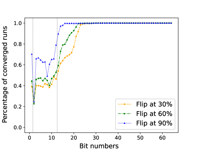
Figure 1: Bit flip sensitivity: averages from all variables.

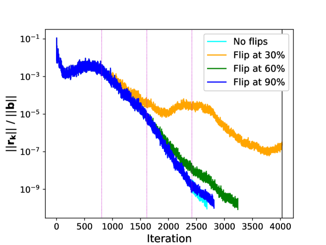
Figure 2: Convergence of the relative residual $\mathbf{||r_{k}||/||b||}$ when the 15th bit of $\beta_{k}$ is flipped for matrix 1138_bus. Purple dotted lines denote flip iterations.

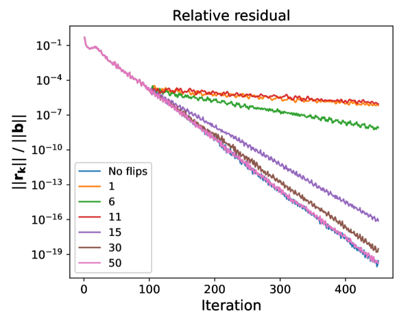
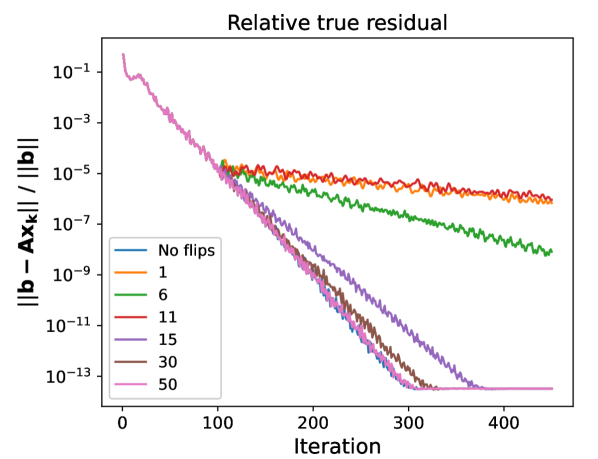
Figure 3: Residual convergence curves when various bits of $\sigma_{k}$ are flipped in the 100th iteration for the matrix bundle1.

3.1 Other effects and error detection

As we have seen in the previous section, silent errors can have significant influence on the convergence of Pipe-PR-CG. Naturally, it can be surmised that other aspects of the procedure might be affected as well. Consequently, some of the effects could be utilized for our ultimate goal - the detection of silent errors. This is the idea of the algorithm-based fault tolerance methods. The fundamental concept of this approach is to derive some criteria of silent error detection from the theoretical or practical knowledge we possess of the algorithm [14]. In our case, we will try to utilize the predict-and-recompute principle which allows us to hide some of the communication.

In Pipe-PR-CG, there are two variables whose value is first predicted using an alternative relation and then recomputed. These are $\nu_{k}$ and $\mathbf{w_{k}}$. We will try to investigate the “gaps” between their predicted version and their recomputed version, i.e., $|\nu_{k}-\nu_{k}^{\prime}|$ and $||\mathbf{w_{k}}-\mathbf{w_{k}^{\prime}}||$, which should be zero in exact arithmetic. Let us now shortly investigate the “cheaper” of these two to compute - the $\nu$-gap.

Figure 4 depicts the $\nu$-gap values when the 15th bit of $\gamma_{k}$ is flipped in the 100th iteration for the matrix bcsstm07. The computation is without preconditioning, with initial guess $\mathbf{x_{0}}$ being a vector of all zeros, and the right-hand side $\mathbf{b}$ is once again such that it holds that $\mathbf{b}=\mathbf{Ae}$. As can be observed, there is a significant outlier among the values in the 101st iteration, i.e., in the very next iteration after the bit flip. This is a promising result which indicates that the $\nu$-gap might be useful for silent error detection and it motivates further exploration into the prospect of utilizing certain quantities for the detection of silent errors in Pipe-PR-CG. The next section studies the possibility of using several variable “gaps” to this end.

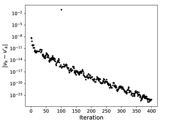
Figure 4: The $\nu$-gap ($|\nu_{k}-\nu_{k}^{\prime}|$) when the 15th bit of $\gamma_{k}$ is flipped in the 100th iteration for the matrix bcsstm07

4 Detecting Silent Errors

In this section, we derive relations which can be effectively used to detect silent errors in Pipe-PR-CG (Algorithm 2). We present several so-called “gaps”, and then employ rounding error analysis to obtain expressions which bound these gaps from above. Subsequently, numerical experiments are performed for each of these gap-bound pairs to judge how effectively they can be utilized to detect silent errors. The idea is that a violation of the bound is a potential indicator of a bit flip having occurred.

As before, we do not include any preconditioning in our derivations or experiments, since this will not affect our primary results or conclusions. In the remainder of the article, “Pipe-PR-CG” thus refers strictly to unpreconditioned Pipe-PR-CG.

We will use a standard model of arithmetic with floating-point numbers. Let the symbol $\circ$ denote one of the operations $\{+,-,\times,\div\}$, $\epsilon$ the machine precision, $a$ and $b$ arbitrary feasible real numbers, and $\text{fp}(\cdot)$ which operation is performed in finite precision. Then, it holds that

$$|\text{fp}(a\circ b)-a\circ b|\leq\epsilon\,|a\circ b|.$$ (1)

Within this framework, it is possible to derive bounds on some of the standard vector operations. Letting $\mathbf{x},\mathbf{y}\in\mathbb{R}^{n}$ and $a\in\mathbb{R}$, we have that

$$||\text{fp}(\mathbf{x}+a\mathbf{y})-(\mathbf{x}+a\mathbf{y})|| \leq\epsilon\,(||\mathbf{x}||+2|a|\,||\mathbf{y}||),$$ (2)

$$||\text{fp}(\langle\mathbf{x},\mathbf{y}\rangle)-\langle\mathbf{x},\mathbf{y}\rangle|| \leq\epsilon\,n\,||\mathbf{x}||\,||\mathbf{y}||,$$ (3)

$$||\text{fp}(\mathbf{Ax})-\mathbf{Ax}|| \leq\epsilon\,c\,||\mathbf{A}||\,||\mathbf{x}||,$$ (4)

where $c$ is a constant depending on specific properties of the matrix $\mathbf{A}$. For instance, it is frequently taken as $c=mn^{1/2}$, where $m$ is the maximum number of nonzeros over the rows of $\mathbf{A}$.

Here, we use $\delta$ to denote a round-off error introduced in a calculation, i.e., the difference between the actual finitely computed result and the exact expression for the variable denoted in the subscript of $\delta$. Taking for instance $\delta_{\sigma_{k}}$ as an example, it holds that $\delta_{\sigma_{k}}=\sigma_{k}-\langle\mathbf{r_{k}},\mathbf{s_{k}}\rangle\leq\epsilon\,n\,||\mathbf{r_{k}}||\,||\mathbf{s_{k}}||$.

4.1 $\nu$-gap

We first investigate the $\nu$-gap mentioned in the previous section, defined as the size of the difference between the predicted value $\nu^{\prime}_{k}$ and the recomputed value $\nu_{k}$ in Pipe-PR-CG, i.e., $|\nu_{k}-\nu^{\prime}_{k}|$. Let us recall how these variables are defined. It holds that

$$\nu_{k}=\langle\mathbf{r_{k}},\mathbf{r_{k}}\rangle,\quad\text{and}\quad\nu^{\prime}_{k}=\nu_{k-1}-2\alpha_{k-1}\sigma_{k-1}+\alpha^{2}_{k-1}\gamma_{k-1},$$

which are mathematically equivalent, i.e., they would be equal if the algorithm was executed in exact arithmetic. As we observed in Figure 4, the $\nu$-gap shows promising potential for silent error detection. However, an issue is how to determine when the value of the $\nu$-gap signals a potential silent error occurrence. One problem is that, as can be seen in Figure 4, the $\nu$-gap can fluctuate. Moreover, even if a silent error influences the $\nu$-gap, nothing guarantees there will always be such a distinct outlier value as in the aforementioned graph. Therefore, it is highly desirable to derive some quantity which bounds the $\nu$-gap from above, and then utilize this bound to determine if the $\nu$-gap indicates the possibility of a silent error occurring by checking whether the $\nu$-gap exceeded the bound.

A bound for the $\nu$-gap was previously derived in [6]. Following the derivation in [6], we can obtain the following bound for the $\nu$-gap:

$$|\nu_{k}-\nu_{k}^{\prime}|\equiv\Delta_{\nu^{\prime}_{k}}\lesssim\epsilon\,(21+6n)(||\mathbf{r_{k-1}}||^{2}+||\mathbf{r_{k}}||^{2}),$$

where the $\lesssim$ indicates that we have dropped terms of order $O(\epsilon^{2})$ and higher. Note that the above bound is slightly tighter than the one previously presented in [6] in that the constants are slightly smaller; this result can be obtained by using different algebraic manipulations.

Given the $\nu$-bound, we now investigate whether it is violated if a bit flip occurs. This is illustrated in the multi-graphs in Figure 5, which depict the behavior of the $\nu$-gap, $|\nu_{k}-\nu_{k}^{\prime}|$, and the $\nu$-bound, $\epsilon\,(21+6n)(||\mathbf{r_{k-1}}||^{2}+||\mathbf{r_{k}}||^{2})$, when the 20th bit is flipped in each variable, for the matrix bcsstm07 (see Table 1). There is one common subplot for the variable $\mathbf{x_{k}}$ and the case of no bit flip occurring during the run, since the resulting graph is the same as flips in $\mathbf{x_{k}}$ have no effect on the values of other variables. The norms $||\mathbf{r_{k-1}}||^{2}$ and $||\mathbf{r_{k}}||^{2}$ were computed using the already calculated $\nu_{k}=\langle\mathbf{r_{k}},\mathbf{r_{k}}\rangle$ and $\nu_{k-1}=\langle\mathbf{r_{k-1}},\mathbf{r_{k-1}}\rangle$. For vector variables ($\mathbf{x_{k}}$, $\mathbf{r_{k}}$, $\mathbf{w^{\prime}_{k}}$, $\mathbf{p_{k}}$, $\mathbf{s_{k}}$, $\mathbf{u_{k}}$, $\mathbf{w_{k}}$) the bit was always flipped in the 100th position of the vector. The right-hand side $\mathbf{b}$ was a vector of all ones, i.e., $\mathbf{b}=\mathbf{e}$.

The iteration range of the figure was chosen to reflect how many iterations are approximately needed to converge for the given problem data. When the $\nu$-gap exceeds the $\nu$-bound, its marker symbol changes to a square. The $\nu$-gap can at times be zero. However, this is not displayed in the figures for the sake of their simplicity. Finally, note that many more experimental runs with different system data were performed in order to judge the behavior of the $\nu$-gap and the $\nu$-bound. The one multi-graph presented here is a representative sample. This holds for all the silent error detection criteria introduced in this section; additional experiments for a different matrix can be found in Appendix B.

Generally, it can be concluded that $\nu$-gap/bound detection works well when the silent error occurs in $\nu^{\prime}_{k},\sigma_{k},\gamma_{k}$, or $\nu_{k}$. It can also seemingly detect errors in the residual $\mathbf{r_{k}}$. However, this does not hold if the flip occurs in the first (sign) bit. This is only logical, as the sign bit is irrelevant for the value of $\nu_{k}=\langle\mathbf{r_{k}},\mathbf{r_{k}}\rangle$, and therefore the $\nu$-gap is not influenced by flips in it.

The bound is violated even for flips in bits of higher number. During the sensitivity experiments in the previous section, it was discovered that flips in bits of number 25 and higher usually do not destroy convergence, as is illustrated by Figure 2. This means that once we employ this criterion in practice, it may raise an alarm even in the case of bit flips which have a negligible effect on convergence. Another noteworthy fact is that for $\mathbf{r_{k}}$ and $\nu^{\prime}_{k}$, the bound is violated at the flip iteration, whereas for $\sigma_{k}$ and $\gamma_{k}$, the violation happens one iteration later. In the case of $\nu_{k}$, the bound is violated both in the flip iteration and the following iteration. Monitoring when our criteria raise an alarm that a silent error has likely occurred is important for its correction. The idea for this correction is that we keep variables from a number of previous iterations or make some checkpoints, and if the flip is detected immediately we can roll back to a state which should not yet be influenced by the error.

In conclusion, the $\nu$-gap/bound criterion seems to be able to reliably detect flips in $\nu^{\prime}_{k},\sigma_{k},\gamma_{k}$, and $\nu_{k}$, as well as in non-sign bits for $\mathbf{r_{k}}$. For other variables a different detection method must be used.

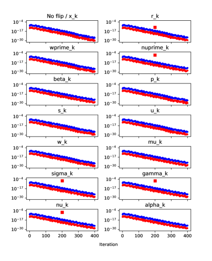
Figure 5: $\nu$-gap (red) and $\nu$-bound (blue) graph, matrix bcsstm07

4.2 $w$-gap

While the $\nu$-gap is a useful tool, ultimately, it seems to function only for a specific subset of variables. Since we aim to be able to detect flips in all Pipe-PR-CG variables, it is necessary to derive additional detection criteria. We can also investigate the gap for the other predicted-and-recomputed quantity, the $\mathbf{w}$-gap, i.e., the size of the difference between the predicted value $\mathbf{w^{\prime}_{k}}$ and the recomputed value $\mathbf{w_{k}}$, which again are equal in exact arithmetic. Note that there is no existing bound on this quantity in the literature.

We now seek to derive a bound for the $\mathbf{w}$-gap. With the symbols $\delta$ once again denoting the rounding errors, it holds that

$$\mathbf{r_{k}}=\mathbf{r_{k-1}}-\alpha_{k-1}\mathbf{s_{k-1}}+\delta_{\mathbf{r_{k}}},$$

$$\mathbf{w^{\prime}_{k}}=\mathbf{w_{k-1}}-\alpha_{k-1}\mathbf{u_{k-1}}+\delta_{\mathbf{w^{\prime}_{k}}},$$ (5)

$$\mathbf{u_{k}}=\mathbf{As_{k}}+\delta_{\mathbf{u_{k}}},$$

$$\mathbf{w_{k}}=\mathbf{Ar_{k}}+\delta_{\mathbf{w_{k}}}.$$

We use these relations to rewrite the expression for $\mathbf{w_{k}}-\mathbf{w^{\prime}_{k}}$ as

$$\mathbf{{w}_{k}}-\mathbf{{w}^{\prime}_{k}} =\mathbf{Ar_{k}}+\delta_{\mathbf{w_{k}}}-(\mathbf{w_{k-1}}-\alpha_{k-1}\mathbf{{u}_{k-1}}+\delta_{\mathbf{w}^{\prime}_{k}})$$

$$=\mathbf{Ar_{k-1}}-\alpha_{k-1}\mathbf{As_{k-1}}+\mathbf{A}{\delta_{\mathbf{r_{k}}}}+\delta_{\mathbf{w_{k}}}-(\mathbf{w_{k-1}}-\alpha_{k-1}\mathbf{{u}_{k-1}}+\delta_{\mathbf{w}^{\prime}_{k}})$$

$$=(\mathbf{Ar_{k-1}}-\mathbf{w_{k-1}})-\alpha_{k-1}(\mathbf{As_{k-1}}-\mathbf{{u}_{k-1}})+\mathbf{A}{\delta_{\mathbf{r_{k}}}}+\delta_{\mathbf{w_{k}}}-\delta_{\mathbf{w}^{\prime}_{k}}$$

$$=-\delta_{\mathbf{{w}_{k-1}}}+\delta_{\mathbf{w_{k}}}+\alpha_{k-1}\delta_{\mathbf{{u}_{k-1}}}+\mathbf{A}{\delta_{\mathbf{r_{k}}}}-\delta_{\mathbf{w}^{\prime}_{k}}.$$

Subsequently, we can take the norm of both sides to obtain the inequality

$$\Delta_{\mathbf{w}^{\prime}_{k}}\equiv||\mathbf{{w}_{k}}-\mathbf{{w}^{\prime}_{k}}||\leq||\delta_{\mathbf{{w}_{k-1}}}||+||\delta_{\mathbf{w_{k}}}||+|\alpha_{k-1}|\,||\delta_{\mathbf{{u}_{k-1}}}||+||\mathbf{A}||\,||\delta_{\mathbf{r_{k}}}||+||\delta_{\mathbf{w}^{\prime}_{k}}||.$$ (6)

We now aim to bound individual terms from (6), starting with the first three of them, i.e., $\delta_{\mathbf{{w}_{k-1}}}$, $\delta_{\mathbf{{w}_{k}}}$, and $\delta_{\mathbf{{u}_{k-1}}}$. Using relations from (4.2) together with (4) yields

$$||\delta_{\mathbf{{w}_{k}}}|| \leq\epsilon\,c\,||\mathbf{A}||\,||\mathbf{r_{k}}||,$$ (7)

$$||\delta_{\mathbf{{w}_{k-1}}}|| \leq\epsilon\,c\,||\mathbf{A}||\,||\mathbf{r_{k-1}}||,$$ (8)

$$||\delta_{\mathbf{{u}_{k-1}}}|| \leq\epsilon\,c\,||\mathbf{A}||\,||\mathbf{s_{k-1}}||,$$ (9)

where $c=mn^{1/2}$, with $m$ the maximum number of nonzero elements in any row of $\mathbf{A}$.

If we rewrite the expression for $\mathbf{r_{k}}$ from (4.2) we obtain that

$$\mathbf{s_{k-1}}=\frac{1}{\alpha_{k-1}}(\mathbf{r_{k-1}}-\mathbf{r_{k}}+\delta_{\mathbf{r_{k}}}),$$

from which we can bound $\mathbf{s_{k}}$ from above as

$$\mathbf{||s_{k-1}}||\leq\frac{1}{|\alpha_{k-1}|}(||\mathbf{r_{k-1}}||+||\mathbf{r_{k}}||+||\delta_{\mathbf{r_{k}}}||).$$ (10)

Now, let us start by bounding $\delta_{\mathbf{r_{k}}}$. The first inequality below is obtained by using relations (4.2) and (3). Then, we use (10), and subsequently rewrite the last term as $O(\epsilon^{2})$, owing to the initial inequality. This yields

$$||\delta_{\mathbf{r_{k}}}|| \leq\epsilon\,(||\mathbf{r_{k-1}}||+2|\alpha_{k-1}|\,||\mathbf{s_{k-1}}||)$$

$$\leq\epsilon\left(||\mathbf{r_{k-1}}||+2|\alpha_{k-1}|\left(\frac{1}{|\alpha_{k-1}|}(||\mathbf{r_{k-1}}||+||\mathbf{r_{k}}||+||\delta_{\mathbf{r_{k}}}||\right)\right)$$

$$\leq\epsilon\,(2||\mathbf{r_{k}}||+3||\mathbf{r_{k-1}}||)+2\,\epsilon\,||\delta_{\mathbf{r_{k}}}||$$

$$\leq 3\,\epsilon\,(||\mathbf{r_{k}}||+||\mathbf{r_{k-1}}||)+O(\epsilon^{2}).$$ (11)

We can bound $\delta_{\mathbf{w^{\prime}_{k}}}$ by first utilizing (4.2) and (3). Then, we use (4.2) again, this time to rewrite the variables inside norms, and, subsequently, we employ the triangle inequality. Finally, we utilize the relations (8) and (9) to rewrite $\epsilon\,||\delta_{\mathbf{{w}_{k-1}}}||$ and $\epsilon\,||\delta_{\mathbf{{u}_{k-1}}}||$ as $O(\epsilon^{2})$, and use properties of the $2$-norm to factor out $||\mathbf{A}||$:

$$||\delta_{\mathbf{w^{\prime}_{k}}}|| \leq\epsilon\,(||\mathbf{{w}_{k-1}}||+2|\alpha_{k-1}|\,||\mathbf{{u}_{k-1}}||)$$

$$=\epsilon\,(||\mathbf{Ar_{k-1}}+\delta_{\mathbf{{w}_{k-1}}}||+2|\alpha_{k-1}|\,||\mathbf{As_{k-1}}+\delta_{\mathbf{{u}_{k-1}}}||)$$

$$\leq\epsilon\,(||\mathbf{Ar_{k-1}}||+||\delta_{\mathbf{{w}_{k-1}}}||+2|\alpha_{k-1}|\,||\mathbf{As_{k-1}}||+||\delta_{\mathbf{{u}_{k-1}}}||)$$

$$\leq\epsilon\,||\mathbf{A}||\,(||\mathbf{r_{k-1}}||+2|\alpha_{k-1}|\,||\mathbf{s_{k-1}}||)+O(\epsilon^{2}).$$ (12)

With each term bounded, we can now substitute from (7) - (12) into (6), and then drop terms of order $O(\epsilon^{2})$ to obtain the final bound for $\Delta_{\mathbf{w}^{\prime}_{k}}$ as

$$\Delta_{\mathbf{w}^{\prime}_{k}} \leq\epsilon\,c\,||\mathbf{A}||\,||\mathbf{r_{k-1}}||+\epsilon\,c\,||\mathbf{A}||\,||\mathbf{r_{k}}||+\epsilon\,c\,|\alpha_{k-1}|\,||\mathbf{A}||\,||\mathbf{s_{k-1}}||$$

$$\quad+3\,\epsilon\,||\mathbf{A}||\,(||\mathbf{r_{k}}||+||\mathbf{r_{k-1}}||)+\epsilon\,||\mathbf{A}||\,(||\mathbf{r_{k-1}}||+2|\alpha_{k-1}|\,||\mathbf{s_{k-1}}||)+O(\epsilon^{2})$$

$$\lesssim\epsilon\,||\mathbf{A}||\,\big{(}(c+3)||\mathbf{r_{k}}||+(c+4)||\mathbf{r_{k-1}}||+(c+2)\,|\alpha_{k-1}|\,||\mathbf{s_{k-1}}||\big{)}.$$

Unlike the $\nu$-bound, this expression contains two terms, $c$ and $||\mathbf{A}||$, which depend on properties of $\mathbf{A}$, and which need to be known prior to the computation if we wish to utilize this bound for silent error detection. We note that a reasonable estimation of $||\mathbf{A}||$ can be obtained from a few iterations of Pipe-PR-CG itself [15]. We also note that an additional inner product is required in the algorithm to compute $||\mathbf{w_{k}-w^{\prime}_{k}}||$.

With the $\mathbf{w}$-bound derived, we can now test its efficacy for silent error detection in Pipe-PR-CG as we did for the $\nu$-bound. There is once again a multi-graph as an example of the behavior, this time depicting the behavior of the $\mathbf{w}$-gap: $||\mathbf{w_{k}}-\mathbf{w^{\prime}_{k}}||$, and the $\mathbf{w}$-bound: $\epsilon\,||\mathbf{A}||\,((c+3)||\mathbf{r_{k}}||+(c+4)||\mathbf{r_{k-1}}||+(c+2)\,|\alpha_{k-1}|\,||\mathbf{s_{k-1}}||)$, when a bit flip occurs in each of the Pipe-PR-CG variables. The norms $||\mathbf{r_{k}}||$, $||\mathbf{r_{k-1}}||$, and $||\mathbf{s_{k-1}}||$ were computed by taking square roots of $|\nu_{k}|$ and $|\gamma_{k}|$, with the absolute value ensuring that the square roots can be taken even if the values of $\nu_{k}$ and $\gamma_{k}$ become negative because of the injected bit flip. The setup of the our experiment is the same as for the $\nu$-gap/bound.

By inspecting Figure 6, we observe that the $\mathbf{w}$-gap/bound seems to work for silent error detection in $\mathbf{r_{k}}$, $\mathbf{w^{\prime}_{k}}$, $\mathbf{u_{k}}$, and $\mathbf{w_{k}}$. On top of that, the experiments showed that the $\mathbf{w}$-gap is also able to detect flips of the sign bit in the residual vector - something the $\nu$-gap was not able to achieve. However, there may be concern whether the $\mathbf{w}$-gap/bound criterion functions properly for matrices with properties which result in large $||\mathbf{A}||$ or the constant $c$, but even in such cases this criterion seems to be reliable for detecting silent errors in the variables above. Once again, depending on the variables, the bound is violated either at the flip iteration or in the very next one. Namely, at the flip iteration for $\mathbf{r_{k}}$ and $\mathbf{w^{\prime}_{k}}$, in the next iteration for $\mathbf{u_{k}}$, and in both for $\mathbf{w_{k}}$.

In conclusion, the detection method based on monitoring violation of the $\mathbf{w}$-bound appears to be functional for $\mathbf{r_{k}}$, $\mathbf{w^{\prime}_{k}}$, $\mathbf{u_{k}}$, and $\mathbf{w_{k}}$. However, let us note that for $\mathbf{r_{k}}$ and $\mathbf{u_{k}}$, it may occasionally be slightly less reliable.

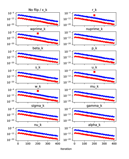
Figure 6: $\mathbf{w}$-gap (red) and $\mathbf{w}$-bound (blue) graph, matrix bcsstm07

4.3 $\mu$-gap

Having investigated both the $\nu$-gap and the $\mathbf{w}$-gap, it is apparent that there are still some Pipe-PR-CG variables for which these two detection methods do not work, namely, $\mathbf{x_{k}}$, $\beta_{k}$, $\mathbf{p_{k}}$, $\mathbf{s_{k}}$, $\mu_{k}$, and $\alpha_{k}$. Therefore, it is necessary to derive another criterion which is not based on monitoring a difference between the predicted value and the recomputed value of some variable, as at this point we have already utilized all two, respectively four, of them. Fortunately, there are other quantities in the Pipe-PR-CG algorithm which should be equal in exact arithmetic. These are $\mu_{k}$ and $\sigma_{k}$, defined as

$$\mu_{k}=\langle\mathbf{p_{k}},\mathbf{s_{k}}\rangle,\quad\text{and}\quad\sigma_{k}=\langle\mathbf{r_{k}},\mathbf{s_{k}}\rangle.$$

Their equality in exact arithmetic holds, because, owing to the relation $\mathbf{p_{k}}=\mathbf{r_{k}}+\beta_{k}\mathbf{p_{k-1}}$ from Pipe-PR-CG, we can rewrite $\mu_{k}$ as

$$\mu_{k}=\langle\mathbf{p_{k}},\mathbf{s_{k}}\rangle=\langle\mathbf{r_{k}}+\beta_{k}\mathbf{p_{k-1}},\mathbf{s_{k}}\rangle,$$

where the inner product $\langle\mathbf{p_{k-1}},\mathbf{s_{k}}\rangle$ is equal to zero. This holds because in exact arithmetic we have that $\mathbf{s_{k}}=\mathbf{Ap_{k}}$, as it originally is in, e.g., HS-CG, and vectors $\mathbf{p_{i}}$, and $\mathbf{p_{j}}$ are $A$-orthogonal for $i\neq j$.

Knowing this, we can define the $\mu$-gap as $\Delta_{\mu^{\prime}_{k}}\equiv|\mu_{k}-\sigma_{k}|$, and derive a bound for it. We use the finite arithmetic relations

$$\mathbf{p_{k}}=\mathbf{r_{k}}+\beta_{k}\mathbf{p_{k-1}}+\delta_{\mathbf{p_{k}}},$$

$$\mu_{k}=\langle\mathbf{p_{k}},\mathbf{s_{k}}\rangle+\delta_{\mu_{k}},$$ (13)

$$\sigma_{k}=\langle\mathbf{r_{k}},\mathbf{s_{k}}\rangle+\delta_{\sigma_{k}}.$$

By utilizing the above expressions, we can write

$$\mu_{k}-\sigma_{k} =\langle\mathbf{p_{k}},\mathbf{s_{k}}\rangle-\langle\mathbf{r_{k}},\mathbf{s_{k}}\rangle+\delta_{\mu_{k}}-\delta_{\sigma_{k}}$$

$$=\langle\mathbf{r_{k}}+\beta_{k}\mathbf{p_{k-1}}+\delta_{\mathbf{p_{k}}},\mathbf{s_{k}}\rangle-\langle\mathbf{r_{k}},\mathbf{s_{k}}\rangle+\delta_{\mu_{k}}-\delta_{\sigma_{k}}$$

$$=\beta_{k}\langle\mathbf{p_{k-1}},\mathbf{s_{k}}\rangle+\langle\delta_{\mathbf{p_{k}}},\mathbf{s_{k}}\rangle+\delta_{\mu_{k}}-\delta_{\sigma_{k}},$$

which, by taking the norm of both sides, yields

$$\Delta_{\mu^{\prime}_{k}} \leq|\beta_{k}|\,|\langle\mathbf{p_{k-1}},\mathbf{s_{k}}\rangle|+|\langle\delta_{\mathbf{p_{k}}},\mathbf{s_{k}}\rangle|+|\delta_{\mu_{k}}|+|\delta_{\sigma_{k}}|$$

$$\leq|\beta_{k}|\,|\langle\mathbf{p_{k-1}},\mathbf{s_{k}}\rangle|+||\delta_{\mathbf{p_{k}}}||\,||\mathbf{s_{k}}||+|\delta_{\mu_{k}}|+|\delta_{\sigma_{k}}|.$$ (14)

Using (3) and (4.3), $|\delta_{\mu_{k}}|$ and $|\delta_{\sigma_{k}}|$ can be bounded as

$$|\delta_{\mu_{k}}| \leq\epsilon\,n\,(||\mathbf{p_{k}}||\,||\mathbf{s_{k}}||),$$ (15)

$$|\delta_{\sigma_{k}}| \leq\epsilon\,n\,(||\mathbf{r_{k}}||\,||\mathbf{s_{k}}||),$$ (16)

and, similarly, owing to (2) and (4.3), we can derive that

$$||\delta_{\mathbf{p_{k}}}||\leq\epsilon\,(||\mathbf{r_{k}}||+2|\beta_{k}|\,||\mathbf{p_{k-1}}||).$$ (17)

Unfortunately, to the authors’ knowledge, there is no method of rewriting the term $\langle\mathbf{p_{k-1}},\mathbf{s_{k}}\rangle$ in a way which does not involve norms of $\mathbf{p_{k-1}}$, $\mathbf{s_{k}}$, or some other variable, as this would greatly diminish tightness of the bound. Therefore, we must keep it in the overall bound of the $\mu$-gap as it is. Thus, by keeping this term and substituting (15), (16), and (17) into (4.3) we obtain that

$$\Delta_{\mu^{\prime}_{k}} \leq|\beta_{k}|\,|\langle\mathbf{p_{k-1}},\mathbf{s_{k}}\rangle|+\epsilon(||\mathbf{r_{k}}||+2|\beta_{k}|\,||\mathbf{p_{k-1}}||)||\mathbf{s_{k}}||$$

$$\quad+\epsilon\,n\,(||\mathbf{p_{k}}||\,||\mathbf{s_{k}}||)+\epsilon\,n\,(||\mathbf{r_{k}}||\,||\mathbf{s_{k}}||)$$

$$\leq|\beta_{k}|\,|\langle\mathbf{p_{k-1}},\mathbf{s_{k}}\rangle|+\epsilon\,||\mathbf{s_{k}}||\big{(}||\mathbf{r_{k}}||+2|\beta_{k}|\,||\mathbf{p_{k-1}}||+n\,(||\mathbf{p_{k}}||+||\mathbf{r_{k}}||)\big{)}.$$

For this expression, two additional inner products are needed in each iteration to compute $\langle\mathbf{p_{k-1}},\mathbf{s_{k}}\rangle$ and $||\mathbf{p_{k}}||$. There is no need to compute the norm $||\mathbf{p_{k-1}}||$ as we can simply keep its value from the previous iteration (or initialization). For future usage, let $B_{\mu^{\prime}_{k}}$ denote the derived bound.

With the $\mu$-bound derived, it is now time to discuss its efficacy for silent error detection in Pipe-PR-CG. Once again, a multi-graph is presented. However, this time the experimental section has two parts. In the first part, we examine figures depicting the $\mu$-gap $\Delta_{\mu^{\prime}_{k}}$ and the $\mu$-bound $B_{\mu^{\prime}_{k}}$. In the second part, their relative difference, $|B_{\mu^{\prime}_{k}}-\Delta_{\mu^{\prime}_{k}}|/B_{\mu^{\prime}_{k}}$, is examined.

The norms $||\mathbf{r_{k}}||$ and $||\mathbf{s_{k}}||$ in $B_{\mu^{\prime}_{k}}$ were again computed by taking square roots of $|\nu_{k}|$ and $|\gamma_{k}|$. For $|\langle\mathbf{p_{k-1}},\mathbf{s_{k}}\rangle|$ and $||\mathbf{p_{k}}||$ additional inner products not appearing in the Pipe-PR-CG algorithm had to be computed. The setup for both of the showcased plots was the same as for the $\nu$-gap and the $\mathbf{w}$-gap.

Now, let us comment on what can be deduced by investigating the first multi-graph in Figure 7, which depicts the $\mu$-gap and the $\mu$-bound side by side. As was done before, if the bound is violated the gap marker turns into a square. However, this time the square is green in order to be easily visible, since for the $\mu$-gap it is always next to a cluster of other gap values.

The first thing we observe is that the $\mu$-gap and bound are sensitive to flips in almost all variables. Another interesting fact is that the $\mu$-bound for many variables seemingly vanishes after the flip. However, this is caused by it being very close to the $\mu$-gap. It is also peculiar that neither the gap nor the bound return to their original level, but instead the values are permanently affected by the flip. This was not the case for the $\nu$- and the $\mathbf{w}$-gaps and bounds. The reason for this is the inner product $|\langle\mathbf{p_{k-1}},\mathbf{s_{k}}\rangle|$ present in the expression of the $\mu$-bound.

As for in which variables the $\mu$-gap/bound method is able to detect flips, it seems that the only ones are $\mathbf{p_{k}}$, $\mu_{k}$, and $\sigma_{k}$. For all three above-mentioned variables, the bound is always violated at the flip iteration. It is also interesting that the reason for this is that for these variables the $\mu$-gap “jumps” one iteration earlier than the $\mu$-bound. For all other variables this happens concurrently, either at the flip iteration or at the very next one. As a final remark, let us also add that, as was the case for the $\nu$-gap, the $\mu$-gap can sometimes be zero.

In conclusion, the $\mu$-gap/bound criterion seems to be well applicable for silent error detection in $\mathbf{p_{k}}$, $\mu_{k}$, and $\sigma_{k}$. However, the quantities themselves are sensitive to flips in other variables as well.

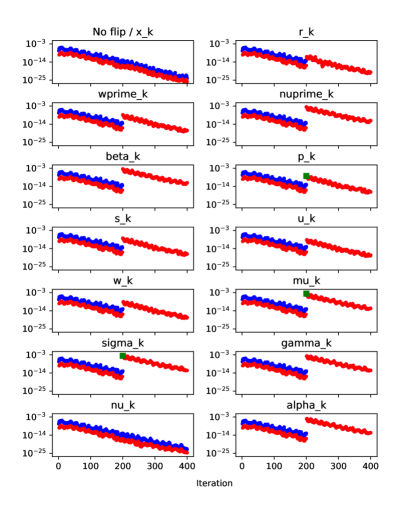
Figure 7: $\mu$-gap (red) and $\mu$-bound (blue) graph, matrix bcsstm07

The problem we are now facing is that there are still some variables for which we do not possess a detection method, namely $\mathbf{x_{k}}$, $\beta_{k}$, $\mathbf{s_{k}}$, and $\alpha_{k}$. However, a straightforward comparison of the gap values and the bound values is not the only way the detection can be done. As was mentioned before, and as can be seen by investigating Figure 7, the $\mu$-gap and the $\mu$-bound are influenced by flips in almost all variables. On top of that, their values after the flip become very close. Therefore, we could try to construct a detection method based on the difference of the $\mu$-gap and the $\mu$-bound. However, it somehow surprisingly turns out that their absolute difference, $|B_{\mu^{\prime}_{k}}-\Delta_{\mu^{\prime}_{k}}|$, steadily decreases despite flips (with the exception of a single jump for $\mathbf{p_{k}}$, $\mu_{k}$, and $\sigma_{k}$). Thus, we try to employ the relative difference, $|B_{\mu^{\prime}_{k}}-\Delta_{\mu^{\prime}_{k}}|/B_{\mu^{\prime}_{k}}$, instead.

There are two reasons for “normalizing” the difference by the $\mu$-bound and not by the $\mu$-gap. The first one is that the $\mu$-gap can sometimes be zero. The second one is that when no flips occur, the $\mu$-bound is guaranteed to be larger than the $\mu$-gap. Therefore, the ratio is going to be “normalized” better.

Figure 8 shows the multi-graph depicting this relative $\mu$-gap/bound difference. The cyan diamond markers show values in the flip iteration and in the one iteration after, i.e., when we would like to be able to detect the flip, so that we can roll back to a close previous state when the variables were still unaffected. The setup and data depicted are the same as in the previous figures of this section.

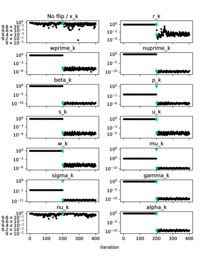
Figure 8: Relative $\mu$-gap/bound difference, $|B_{\mu^{\prime}_{k}}-\Delta_{\mu^{\prime}_{k}}|/B_{\mu^{\prime}_{k}}$, matrix bcsstm07

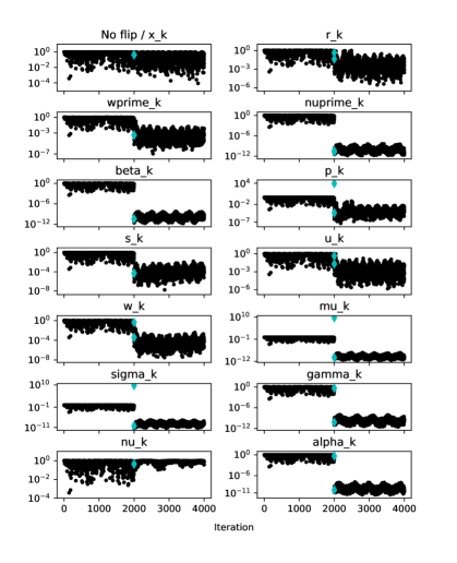
Figure 13: Relative $\mu$-gap/bound difference, $|B_{\mu^{\prime}_{k}}-\Delta_{\mu^{\prime}_{k}}|/B_{\mu^{\prime}_{k}}$, matrix nos7

At first glance, we immediately observe that the effect of the flip is quite significant for all variables besides $\nu_{k}$. Either at the iteration of the flip, one later, or both, there is a significant jump of the value. On top of that, for the three variables ($\mathbf{p_{k}}$, $\mu_{k}$, $\sigma_{k}$), where we were able to detect flips just by the bound violation, the $\mu$-gap/bound relative difference is greater than 1 at the flip iteration, a clear indication that a flip has occurred. Unfortunately, for matrices with higher condition numbers the level of the ratio $|B_{\mu^{\prime}_{k}}-\Delta_{\mu^{\prime}_{k}}|/B_{\mu^{\prime}_{k}}$ may not be so close to one as in Figure 8. This is visible in Figure 13 in Appendix B where the values of the ratio for matrix nos7 falls up to the level of $1\mathrm{e}{-10}$. The values there are altered by the flip, but it can be observed that for vector variables the diamond markers still largely remain in the same value range as when no bits were flipped. However, there is really only one vector variable, $\mathbf{s_{k}}$, which is not covered by the previous detection methods, and the relative $\mu$-gap/bound difference criterion seems to mostly work for it. This can be also seen in Figure 13. Nonetheless, we have also encountered cases where the reliability of this criterion for $\mathbf{s_{k}}$ is borderline.

When it comes to this approach it is also important to investigate at what level the values of the studied ratio $|B_{\mu^{\prime}_{k}}-\Delta_{\mu^{\prime}_{k}}|/B_{\mu^{\prime}_{k}}$ are when no flips occur, because we need to set some threshold to determine whether to raise an alarm that a silent error has likely appeared or not. If we set the threshold too close to 1 we might get a lot of false positive detections. On the other hand, setting it too low might result in a lot of false negatives. For some matrices, e.g., bcsstm07, the values lie very close to 1. However, it seems that higher condition number leads to a decrease of the ratio, e.g., for the matrix nos7 in Appendix B the values are as low as $1\mathrm{e}{-4}$. This indicates that choosing a suitable value of the threshold could be a rather complex and data dependent problem.

The greatest strength of the relative $\mu$-gap/bound difference approach is that it encompasses almost all of the Pipe-PR-CG variables, albeit with some above-mentioned data-related exceptions. However, a disadvantage is that, unlike in the case of the bound violation methods, there is nothing to directly compare the values to, so we have to set some detection threshold.

4.4 Summary of detection methods

We have investigated four methods for silent error detection in Pipe-PR-CG. We summarize their efficacy in terms of whether or not they have the potential to reliably detect bit flips in a given variable in Table 2, with rows representing each of the Pipe-PR-CG variables. The symbol ✓denotes that the method is able to reliably detect flips in the variable, while $\circ$ denotes that the method is, for the given variable, somehow functional, but either not in all cases or there are some specific circumstances under which it is not able to detect the injected error, e.g., the $\nu$-gap/bound criterion not working for sign flips in the residual vector $\mathbf{r_{k}}$.

We can see from the table that the only variable which is not covered by any of the detection methods is the solution vector $\mathbf{x_{k}}$. The reason for this is that $\mathbf{x_{k}}$ appears only in its own relation, and thus it does affect any other variable. Therefore, for silent error detention in $\mathbf{x_{k}}$, a redundancy approach is unfortunately needed. Besides that, we may not posses a robust detection method for flips in $\mathbf{s_{k}}$. Nonetheless, in the worst case, the redundancy approach can be applied here as well if it turns out that detection by the relative $\mu$-gap/bound difference is truly unreliable. For all other variables we should be able to detect silent errors reasonably well.

We note that if the computation of additional inner products and constants necessary for the bounds would in some case be too expensive, it is also possible to construct a set of detection criteria based just on the values of the gaps alone. For instance, we could monitor a moving average of gap value differences between iterations. Nonetheless, it is important to keep in mind that for this approach to function we must somehow deal with iterations where any of the gaps are zero. It would also require us to set some threshold to determine when to raise an alarm that a silent error has likely occurred.

Variable	$\nu$-gap/bound	$\mathbf{w}$-gap/bound	$\mu$-gap/bound	$|B_{\mu^{\prime}_{k}}-\Delta_{\mu^{\prime}_{k}}|/B_{\mu^{\prime}_{k}}$
$\mathbf{x_{k}}$
$\mathbf{r_{k}}$	$\circ$	✓		$\circ$
$\mathbf{w^{\prime}_{k}}$		✓		$\circ$
$\nu^{\prime}_{k}$	✓			✓
$\beta_{k}$				✓
$\mathbf{p_{k}}$			✓	✓
$\mathbf{s_{k}}$				$\circ$
$\mathbf{u_{k}}$		✓		$\circ$
$\mathbf{w_{k}}$		✓		$\circ$
$\mu_{k}$			✓	✓
$\sigma_{k}$	✓		✓	✓
$\gamma_{k}$	✓			✓
$\nu_{k}$	✓
$\alpha_{k}$				✓

Table 2: Efficacy of detection methods for Pipe-PR-CG variables

5 Fault-tolerant Pipe-PR-CG

We now aim to test how well our criteria can detect silent errors in practice. We perform a large numerical experiment examining the performance of the criteria on a large sample of test runs, both with and without bit flips. The experiment was performed for each of the Pipe-PR-CG variables with the exception of $\mathbf{x_{k}}$, since none of the methods work for this variable. It is also worth noting that the experiment was performed for each of the variables separately, so that eventual outliers can be identified more easily.

For all variables, the testing was done using the first eight matrices in Table 1. For each variable and each of these matrices, 800 runs with a single bit flip and 200 without a bit flip were performed. The bit number was chosen randomly from 1 to 64. For vectors, the flip occurred in a random index from $[1,n]$, where $n$ is the problem dimension. The flip iteration $\tau$ was chosen randomly from $0.1\varphi$ to $0.9\varphi$, where $\varphi$ is the number of iterations needed to converge for the given matrix and right-hand side when no flips occur. This was computed before each tainted run. The stopping criterion was always, for both untainted as well as tainted runs, such that it must hold that $||\mathbf{r_{k}}||/||\mathbf{b}||<1\mathrm{e}{-10}$. The right-hand side $\mathbf{b}$ was a random vector from a uniform distribution over $[0,1)$. A run tainted by a bit flip was deemed as convergent if it reached the stopping criteria within $1.5\varphi$ iterations. The initial guess $\mathbf{x_{0}}$ was always a vector of all zeros. Runs with an overflow error were not counted, because such errors are no longer silent. For this reason, the total number of runs recorded for each matrix is slightly lower than the above-stated 1000 performed. When possible, the norms appearing in the code were calculated using the already computed quantities, such as $\nu_{k}$ for $||\mathbf{r_{k}}||$ or $\gamma_{k}$ for $||\mathbf{s_{k}}||$. The only exception was the norm $||\mathbf{r_{k}}||$ used for the stopping criterion which was not computed utilizing $\nu_{k}$, so that the convergence can be evaluated more independently from the detection criteria.

Let us now recall what our four detection methods are. If any of the inequalities

• $|\nu_{k}-\nu_{k}^{\prime}|>\epsilon\,(21+6n)(||\mathbf{r_{k-1}}||^{2}+||\mathbf{r_{k}}||^{2})$,

• $||\mathbf{w_{k}-w^{\prime}_{k}}||>\epsilon\,||\mathbf{A}||\,\big{(}(c+3)||\mathbf{r_{k}}||+(c+4)||\mathbf{r_{k-1}}||+(c+2)\,|\alpha_{k-1}|\,||\mathbf{s_{k-1}}||\big{)}$,

• $\Delta_{\mu^{\prime}_{k}}\equiv|\mu_{k}-\sigma_{k}|\newline >|\beta_{k}|\,|\langle\mathbf{p_{k-1}},\mathbf{s_{k}}\rangle|+\epsilon\,||\mathbf{s_{k}}||\big{(}||\mathbf{r_{k}}||+2|\beta_{k}|\,||\mathbf{p_{k-1}}||+n\,(||\mathbf{p_{k}}||+||\mathbf{r_{k}}||)\big{)}\eqqcolon B_{\mu^{\prime}_{k}}$,

• $|B_{\mu^{\prime}_{k}}-\Delta_{\mu^{\prime}_{k}}|/B_{\mu^{\prime}_{k}}<\text{threshold}$,

held, an alarm was raised. We call these four criteria working together a detection set. In the experiment, there were two detection sets with a different threshold for the relative $\mu$-gap/bound difference criterion to evaluate how the detection behavior changes with the threshold. The threshold values were chosen based on experiments from the fourth chapter. Specifically, the levels $5\mathrm{e}{-1}$ and $1\mathrm{e}{-4}$ were chosen, as they seemed to be close to the lower limit of values of the relative $\mu$-gap/bound difference, $|B_{\mu^{\prime}_{k}}-\Delta_{\mu^{\prime}_{k}}|/B_{\mu^{\prime}_{k}}$, for matrices 1138_bus and nos7 when no flips occur. The two detection sets with different thresholds for the fourth relative $\mu$-gap/bound difference-based criterion were both evaluated simultaneously during each run. Therefore, we can directly compare how they perform for identical data.

The sequence of steps in the experiment was following:

1. For untainted runs, a right-hand side vector $\mathbf{b}$ is generated, then the computation is performed and it is noted whether an alarm was raised. The two detection sets using the two different thresholds for the $|B_{\mu^{\prime}_{k}}-\Delta_{\mu^{\prime}_{k}}|/B_{\mu^{\prime}_{k}}$ criterion are both checked during the run and they each posses their own alarm.

2. For tainted runs, a right-hand side vector $\mathbf{b}$ is generated, and subsequently an untainted computation is performed to obtain the number of iterations $\varphi$ needed to converge. Afterwards, the flip iteration $\tau$, bit number, and vector flip index are generated. Then, a tainted run is performed with these inputs. As was the case for the untainted runs, both detection sets are monitored during the computation. Once again, this is done so that they can be better compared against each other, since they examine the same data. If during the run one of the two detection sets raises its alarm, it is noted at what iteration $\rho_{i}$, $i\in\{1,2\}$, that first was. Later alarms are not taken into account. Besides the first alarm iterations, it is also monitored whether the run converged within the $1.5\varphi$ iterations or not.

Runs were sorted into one of six categories:

• true positive (tp): Flip occurred, did prevent convergence, alarm was raised.

• special positive (sp): Bit flip occurred, did not prevent convergence, alarm was raised.

• false positive (fp): No flip occurred, alarm was raised.

• true negative (tn): No flip occurred, no alarm was raised.

• special negative (sn): Flip occurred, did not prevent convergence, no alarm raised.

• false negative (fn): Flip occurred, did prevent convergence, no alarm raised.

The same categorization was used in [14]. As mentioned above, if in a tainted run any of the four criteria within the detection sets raised an alarm it was noted at what iteration ($\rho_{1}$ for the first detection set and $\rho_{2}$ for the second detection set) this first occurred. The values $\rho_{i}$ were initialized as $\infty$. Thus, if the detection set did not raise an alarm during the run its $\rho_{i}$ value remained so after the computation had concluded. To classify runs, we compared the flip iteration $\tau$ and $\rho_{i}$, receiving the following options:

1. If $\rho_{i}<\tau$, we count this as false positive,

2. If $\rho_{i}\in\{\tau,\tau+1\}$, we count this as true/special positive based on whether the run converged,

3. If $\rho_{i}>\tau+1$, we count this as false/special negative based on whether the run converged.

Runs without a bit flip were categorized either as true negative or false positive based on whether or not an alarm was raised.

The output of the experiment is presented below in Table 3, which contains the sum of all runs over the individual variables. Results for each of the 13 variables separately can be found in Appendix C. The most crucial result is that we were generally able to detect an overwhelming majority of bit flips which would ruin convergence. Important also is the fact that there was no variable which would stick out as seriously problematic for our detection methods. Moreover, the number of false positive runs was (for both thresholds) very close for all variables.

However, there were differences in the overall number of detected errors which would not destroy convergence (sp/sn). The one variable which stands out is $\mathbf{s_{k}}$, for which the number of special negative runs was considerably larger than for any other variable (see Table 10). This was most likely caused by the fact that for $\mathbf{s_{k}}$ only the relative $\mu$-gap/bound difference criterion works, and even then, it is not fully reliable, as previously mentioned. Nonetheless, a majority of the undetected flips were special negative, thus they did not destroy convergence, and it can be seen that the number of false negatives is for $\mathbf{s_{k}}$ quite acceptable. Notable also is the fact that in the case of scalar variables for which one of the gap/bound detection methods works ($\nu^{\prime}_{k}$, $\mu_{k}$, $\sigma_{k}$, $\gamma_{k}$, and $\nu_{k}$) we were able to detect a large portion of the convergence-preserving silent errors. This can be observed in Table 7 and in Tables 13 to 16.

For most matrices, there were no or almost no false positives. Notable outliers are nos7 and 1138_bus. Interestingly, these two matrices along with bcsstk05 and bcsstm07 are all in the upper half of our sample when it comes to condition number. This leads to the conclusion that the threshold value should be ideally chosen proportionally to the condition number of the matrix. We note that false positive detections are caused only by the criterion utilizing the relative difference of the $\mu$-gap and the $\mu$-bound. The three bound violation criteria raise the alarm only when a bit flip truly occurs.

In conclusion, our detection criteria were able to detect silent errors reasonably well, and for the vast majority of the non-detected bit flips the algorithm managed to recover and converge within our set iteration range.

matrix	threshold	tp	sp	fp	tn	sn	fn
1138_bus	$5\mathrm{e}{-1}$	1532	4125	2681	1652	2844	2
	$1\mathrm{e}{-4}$	1732	4509	0	2600	3989	6
bcsstm07	$5\mathrm{e}{-1}$	939	6342	2	2600	2960	3
	$1\mathrm{e}{-4}$	940	5710	0	2600	3593	3
bundle1	$5\mathrm{e}{-1}$	833	5213	0	2600	4088	1
	$1\mathrm{e}{-4}$	833	4554	0	2600	4747	1
wathen120	$5\mathrm{e}{-1}$	771	5331	0	2600	4113	2
	$1\mathrm{e}{-4}$	771	4769	0	2600	4675	2
bcsstk05	$5\mathrm{e}{-1}$	2991	4793	348	2324	2314	5
	$1\mathrm{e}{-4}$	2999	4186	0	2600	2980	10
gr_30_30	$5\mathrm{e}{-1}$	964	6479	0	2600	2783	2
	$1\mathrm{e}{-4}$	964	5900	0	2600	3362	2
nos7	$5\mathrm{e}{-1}$	0	0	12823	0	0	0
	$1\mathrm{e}{-4}$	1381	2881	3843	1229	3485	4
crystm01	$5\mathrm{e}{-1}$	799	5896	0	2600	3564	1
	$1\mathrm{e}{-4}$	799	5292	0	2600	4168	1
$\sum$	$5\mathrm{e}{-1}$	8829	38179	15854	16976	22666	16
	$1\mathrm{e}{-4}$	10419	37801	3843	19429	30999	29

Table 3: Detection performance, sum over all variables

The combination of our detection methods is able to reliably detect majority of silent errors which would destroy convergence of Pipe-PR-CG. The problem at hand is now how to correct these errors. The approach we present here is to perform a so-called rollback when the alarm is raised. Rolling back essentially means to “return” the computation to an uncorrupted state before the detected silent error has occurred. Therefore, in our case, to recover the computation we have to “return” two iterations back, since our detection methods raise the alarm either at the iteration when the error has occurred or one iteration later. This recovery approach was previously proposed in other studies investigating detection and correction of silent errors, e.g., in [14].

Algorithm 4 gives the resulting Fault-Tolerant Pipelined Predict-and-Recompute Conjugate Gradient algorithm (FT-Pipe-PR-CG), which includes the detection and correction of silent errors. We have also explicitly incorporated here the redundancy detection approach for $\mathbf{x_{k}}$. Inputs of the algorithm include, aside from the standard problem data $\mathbf{A}$, $\mathbf{b}$, and $\mathbf{x_{0}}$, the constants $||\mathbf{A}||$, $n$, $\epsilon$, and $c$, necessary for evaluation of the bounds, and the threshold value $T$ used in the $|B_{\mu^{\prime}_{k}}-\Delta_{\mu^{\prime}_{k}}|/B_{\mu^{\prime}_{k}}$ criterion.

If the alarm is raised we call a Recover() procedure (Algorithm 3) to perform the two iteration rollback and we mark the iteration $k+2$ as “corrected”; otherwise, if the detection was falsely positive, the alarm would be raised again indefinitely every two iterations. Although it may theoretically happen that another silent fault appears in an iteration marked as corrected, the probability of this is rather low, since silent errors are a rare event [9]. However, in cases where there is an extremely large number of false positive detections, this may be a problem. We later propose a remedy.

In FT-Pipe-PR-CG it is necessary to compute three additional inner products, $\langle\mathbf{w_{k}-w^{\prime}_{k}},\mathbf{w_{k}-w^{\prime}_{k}}\rangle$, $\langle\mathbf{p_{k-1}},\mathbf{s_{k}}\rangle$, and $\langle\mathbf{p_{k}},\mathbf{p_{k}}\rangle$, which do not appear in the basic Pipe-PR-CG algorithm, for the sake of our detection criteria. Nonetheless, it is possible to couple their computation with the other inner products in line 9 of Algorithm 4, and, aside from $\langle\mathbf{w_{k}-w^{\prime}_{k}},\mathbf{w_{k}-w^{\prime}_{k}}\rangle$, there is no serial dependence on the matrix-vector multiplications. Therefore, the communication-hiding and pipelining properties of Pipe-PR-CG are, to a certain degree, preserved. Note that the procedure stated below is presented merely as a pseudocode.

The advantage of the rollback correction approach is that the algorithm is able to universally recover from any detected silent error, no matter what variable it occurred in. The disadvantage is that we need to allocate extra memory for storing the variables from iterations $k-2$ and $k-3$.

Algorithm 3 Recover procedure of FT-Pipe-PR-CG

1:procedure Recover($\cdot$)

2:     $\mathbf{x_{k}}=\mathbf{x_{k-2}},\quad\mathbf{x_{k-1}}=\mathbf{x_{k-3}}$, $\quad\mathbf{r_{k}}=\mathbf{r_{k-2}},\,\,\quad\mathbf{r_{k-1}}=\mathbf{r_{k-3}}$

3:     $\mathbf{w^{\prime}_{k}}=\mathbf{w^{\prime}_{k-2}},\>\,\,\mathbf{w^{\prime}_{k-1}}=\mathbf{w^{\prime}_{k-3}}$, $\quad\nu^{\prime}_{k}=\nu^{\prime}_{k-2},\quad\,\;\nu^{\prime}_{k-1}=\nu^{\prime}_{k-3}$

4:     $\beta_{k}=\beta_{k-2},\quad\;\beta_{k-1}=\beta_{k-3}$, $\quad\mathbf{p_{k}}=\mathbf{p_{k-2}},\;\>\,\;\mathbf{p_{k-1}}=\mathbf{p_{k-3}}$

5:     $\mathbf{s_{k}}=\mathbf{s_{k-2}},\,\,\quad\mathbf{s_{k-1}}=\mathbf{s_{k-3}}$, $\quad\mathbf{u_{k}}=\mathbf{u_{k-2}},\;\,\,\;\mathbf{u_{k-1}}=\mathbf{u_{k-3}}$

6:     $\mathbf{w_{k}}=\mathbf{w_{k-2}},\;\;\mathbf{w_{k-1}}=\mathbf{w_{k-3}}$, $\quad\mu_{k}=\mu_{k-2},\quad\>\mu_{k-1}=\mu_{k-3}$

7:     $\sigma_{k}=\sigma_{k-2},\quad\>\sigma_{k-1}=\sigma_{k-3}$, $\quad\gamma_{k}=\gamma_{k-2},\quad\>\gamma_{k-1}=\gamma_{k-3}$

8:     $\nu_{k}=\nu_{k-2},\quad\,\>\nu_{k-1}=\nu_{k-3}$, $\quad\alpha_{k}=\alpha_{k-2},\quad\alpha_{k-1}=\alpha_{k-3}$

9:end procedure

Algorithm 4 Fault-Tolerant Pipelined Predict-and-Recompute Conjugate
Gradient: FT-Pipe-PR-CG

1:procedure FT-Pipe-PR-CG($\mathbf{A},\mathbf{b},\mathbf{x_{0}}$, $||\mathbf{A}||$, $n$, $\epsilon$, $c$, $T$)

2:     INITIALIZE()

3:     for $k=1,2,\dots$ do

4:         $\mathbf{x_{k}}=\mathbf{x_{k-1}}+\alpha_{k-1}\mathbf{p_{k-1}},\quad\mathbf{\tilde{x}_{k}}=\mathbf{x_{k-1}}+\alpha_{k-1}\mathbf{p_{k-1}}$

5:         if $\mathbf{x_{k}\neq\tilde{x}_{k}}$ then go to 4

6:         $\mathbf{r_{k}}=\mathbf{r_{k-1}}-\alpha_{k-1}\mathbf{s_{k-1}},\quad\mathbf{w^{\prime}_{k}}=\mathbf{w_{k-1}}-\alpha_{k-1}\mathbf{u_{k-1}}$

7:         $\nu^{\prime}_{k}=\nu_{k-1}-2\alpha_{k-1}\sigma_{k-1}+\alpha^{2}_{k-1}\gamma_{k-1},\quad\beta_{k}=\nu^{\prime}_{k}/\nu_{k-1}$

8:         $\mathbf{p_{k}}=\mathbf{r_{k}}+\beta_{k}\mathbf{p_{k-1}},\quad\mathbf{s_{k}}=\mathbf{w^{\prime}_{k}}+\beta_{k}\mathbf{s_{k-1}},\quad\mathbf{u_{k}}=\mathbf{As_{k}},\quad\mathbf{w_{k}}=\mathbf{Ar_{k}}$

9:         $\mu_{k}=\langle\mathbf{p_{k}},\mathbf{s_{k}}\rangle,\quad\sigma_{k}=\langle\mathbf{r_{k}},\mathbf{s_{k}}\rangle,\quad\gamma_{k}=\langle\mathbf{s_{k}},\mathbf{s_{k}}\rangle,\quad\nu_{k}=\langle\mathbf{r_{k}},\mathbf{r_{k}}\rangle$

10:         $\alpha_{k}=\nu_{k}/\mu_{k}$

11:         $\Delta_{\nu^{\prime}_{k}}=|\nu_{k}-\nu^{\prime}_{k}|,\quad\Delta_{\mathbf{w}^{\prime}_{k}}=||\mathbf{w_{k}-w^{\prime}_{k}}||,\quad\Delta_{\mu^{\prime}_{k}}=|\mu_{k}-\sigma_{k}|$

12:         $B_{\nu^{\prime}_{k}}=\epsilon\,(21+6n)(||\mathbf{r_{k-1}}||^{2}+||\mathbf{r_{k}}||^{2})$

13:         $B_{\mathbf{w}^{\prime}_{k}}=\epsilon\,||\mathbf{A}||\,((c+3)||\mathbf{r_{k}}||+(c+4)||\mathbf{r_{k-1}}||+(c+2)\,|\alpha_{k-1}|\,||\mathbf{s_{k-1}}||)$

14:         $B_{\mu^{\prime}_{k}}=|\beta_{k}|\,|\langle\mathbf{p_{k-1}},\mathbf{s_{k}}\rangle|+\epsilon\,||\mathbf{s_{k}}||(||\mathbf{r_{k}}||+2|\beta_{k}|\,||\mathbf{p_{k-1}}||+n\,(||\mathbf{p_{k}}||+||\mathbf{r_{k}}||))$

15:         if $\Delta_{\nu^{\prime}_{k}}>B_{\nu^{\prime}_{k}}$ or $\Delta_{\mathbf{w}^{\prime}_{k}}>B_{\mathbf{w}^{\prime}_{k}}$ or $\Delta_{\mu^{\prime}_{k}}>B_{\mu^{\prime}_{k}}$ or $|B_{\mu^{\prime}_{k}}-\Delta_{\mu^{\prime}_{k}}|/B_{\mu^{\prime}_{k}}<T$

16:              if $k$ is not marked as corrected

17:                  Recover(), mark $k+2$ as corrected

18:              end if

19:         end if

20:     end for

21:end procedure

6 An Adaptive Threshold Approach

FT-Pipe-PR-CG should be able to reliably detect and correct the majority of silent errors significant for convergence. However, in the previous section (e.g., Table 3) we have observed that for some matrices there were many runs which resulted in false positives. Moreover, the experiment was categorizing the runs based only on the first raising of the alarm. Hence, in some problematic cases there may potentially be a large number of false positive detections during the computation. This would cause us to perform many extra iterations due to the rollback recovery. However, we have also seen that the number of false positives decreases with the value of the threshold parameter. This is a fact we could try to utilize.

The idea we propose here is to adapt the value of the threshold $T$ during the run of the algorithm to reflect how many times the alarm was raised. As was mentioned, silent errors are rather rare events, so if the alarm is raised many times we can safely assume that in most cases we did not truly detect a fault. In such a situation it may be beneficial to lower the value of the threshold $T$ to reduce the number of false positive detections by the relative $\mu$-gap/bound difference criterion. This concept is presented below in Algorithm 5 as the adaptive fault-tolerant Pipe-PR-CG (AFT-Pipe-PR-CG). Here we multiply $T$ by an adaptation parameter $a\in(0,1)$ each time the alarm is raised by the $|B_{\mu^{\prime}_{k}}-\Delta_{\mu^{\prime}_{k}}|/B_{\mu^{\prime}_{k}}$ criterion. Note that it is also possible to increase the threshold when there is a large number of iterations without any alarm. But in that case, it is necessary to set some upper limit for $T$.

Not only does the adaptive algorithm potentially greatly reduce the number of false positive detections, it also allows us to eliminate the iteration marking. In FT-Pipe-PR-CG, if the alarm was raised at some iteration $k$ we have marked iteration $k+2$ as corrected, so that the procedure cannot get stuck in a loop. However, this can be caused only by the relative $\mu$-gap/bound difference criterion. As was mentioned earlier, the three bound violation criteria raise the alarm only when a silent error truly occurs, i.e., they do not cause false positive detections. Thus, the procedure cannot get stuck because one of these criteria will indefinitely force a recovery in some iteration. The relative $\mu$-gap/bound difference criterion could do this, but now, each time this method raises the alarm the threshold is lowered. Therefore, eventually it will hold that $T<|B_{\mu^{\prime}_{k}}-\Delta_{\mu^{\prime}_{k}}|/B_{\mu^{\prime}_{k}}$, and the procedure will continue.

Figure 9 shows the process of threshold adaptation for the matrix nos7 and right-hand side $\mathbf{b=e}$. The adaptivity parameter $a$ was in the presented run set to $0.1$. The initial threshold value was $5\mathrm{e}{-1}$, the higher value used in the detection performance experiment earlier in this section. Next to the variable names, it is noted how many recoveries, i.e., also detections, there were in total during the computation. This number also includes alarms raised after the bit flip by criteria other than the threshold violation by the relative $\mu$-gap/bound difference. Therefore, for some variables, e.g., $\mathbf{w^{\prime}_{k}}$, the number of threshold adaptations was one less than the number of total detections indicated in the figures. A violation of the threshold by the $|B_{\mu^{\prime}_{k}}-\Delta_{\mu^{\prime}_{k}}|/B_{\mu^{\prime}_{k}}$ ratio in the flip iteration or one iteration later is denoted by the diamond marker turning dark blue.

We observe that AFT-Pipe-PR-CG seems to be able to suitably adapt the threshold, so that the number of false positive detections is reduced, but at the same time the reliability of the detection is not destroyed. Notable also is that the ratio $|B_{\mu^{\prime}_{k}}-\Delta_{\mu^{\prime}_{k}}|/B_{\mu^{\prime}_{k}}$ no longer “jumps down” as we have observed in Figure 8. This is because of the recovery procedure.

Algorithm 5 Adaptive Fault-Tolerant Pipelined Predict-and-Recompute
Conjugate Gradient: AFT-Pipe-PR-CG

1:procedure AFT-Pipe-PR-CG($\mathbf{A},\mathbf{b},\mathbf{x_{0}}$, $||\mathbf{A}||$, $n$, $\epsilon$, $c$, $T$, $a$)

2:     INITIALIZE()

3:     for $k=1,2,\dots$ do

4:         $\mathbf{x_{k}}=\mathbf{x_{k-1}}+\alpha_{k-1}\mathbf{p_{k-1}},\quad\mathbf{\tilde{x}_{k}}=\mathbf{x_{k-1}}+\alpha_{k-1}\mathbf{p_{k-1}}$

5:         if $\mathbf{x_{k}\neq\tilde{x}_{k}}$ then go to 4

6:         $\mathbf{r_{k}}=\mathbf{r_{k-1}}-\alpha_{k-1}\mathbf{s_{k-1}},\quad\mathbf{w^{\prime}_{k}}=\mathbf{w_{k-1}}-\alpha_{k-1}\mathbf{u_{k-1}}$

7:         $\nu^{\prime}_{k}=\nu_{k-1}-2\alpha_{k-1}\sigma_{k-1}+\alpha^{2}_{k-1}\gamma_{k-1},\quad\beta_{k}=\nu^{\prime}_{k}/\nu_{k-1}$

8:         $\mathbf{p_{k}}=\mathbf{r_{k}}+\beta_{k}\mathbf{p_{k-1}},\quad\mathbf{s_{k}}=\mathbf{w^{\prime}_{k}}+\beta_{k}\mathbf{s_{k-1}},\quad\mathbf{u_{k}}=\mathbf{As_{k}},\quad\mathbf{w_{k}}=\mathbf{Ar_{k}}$

9:         $\mu_{k}=\langle\mathbf{p_{k}},\mathbf{s_{k}}\rangle,\ \sigma_{k}=\langle\mathbf{r_{k}},\mathbf{s_{k}}\rangle,\ \gamma_{k}=\langle\mathbf{s_{k}},\mathbf{s_{k}}\rangle,\ \nu_{k}=\langle\mathbf{r_{k}},\mathbf{r_{k}}\rangle$

10:         $\alpha_{k}=\nu_{k}/\mu_{k}$

11:         $\Delta_{\nu^{\prime}_{k}}=|\nu_{k}-\nu^{\prime}_{k}|,\quad\Delta_{\mathbf{w}^{\prime}_{k}}=||\mathbf{w_{k}-w^{\prime}_{k}}||,\quad\Delta_{\mu^{\prime}_{k}}=|\mu_{k}-\sigma_{k}|$

12:         $B_{\nu^{\prime}_{k}}=\epsilon\,(21+6n)(||\mathbf{r_{k-1}}||^{2}+||\mathbf{r_{k}}||^{2})$

13:         $B_{\mathbf{w}^{\prime}_{k}}=\epsilon\,||\mathbf{A}||\,((c+3)||\mathbf{r_{k}}||+(c+4)||\mathbf{r_{k-1}}||+(c+2)\,|\alpha_{k-1}|\,||\mathbf{s_{k-1}}||)$

14:         $B_{\mu^{\prime}_{k}}=|\beta_{k}|\,|\langle\mathbf{p_{k-1}},\mathbf{s_{k}}\rangle|+\epsilon\,||\mathbf{s_{k}}||(||\mathbf{r_{k}}||+2|\beta_{k}|\,||\mathbf{p_{k-1}}||+n\,(||\mathbf{p_{k}}||+||\mathbf{r_{k}}||))$

15:         if $\Delta_{\nu^{\prime}_{k}}>B_{\nu^{\prime}_{k}}$ or $\Delta_{\mathbf{w}^{\prime}_{k}}>B_{\mathbf{w}^{\prime}_{k}}$ or $\Delta_{\mu^{\prime}_{k}}>B_{\mu^{\prime}_{k}}$ or $|B_{\mu^{\prime}_{k}}-\Delta_{\mu^{\prime}_{k}}|/B_{\mu^{\prime}_{k}}<T$

16:              Recover()

17:              if $|B_{\mu^{\prime}_{k}}-\Delta_{\mu^{\prime}_{k}}|/B_{\mu^{\prime}_{k}}<T$ then $T=a\cdot T$

18:         end if

19:     end for

20:end procedure

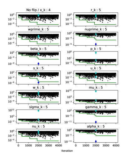
Figure 9: Adaptive threshold $T$ for $a=0.1$ (green) and the relative $\mu$-gap/bound difference, $|B_{\mu^{\prime}_{k}}-\Delta_{\mu^{\prime}_{k}}|/B_{\mu^{\prime}_{k}}$, (black), matrix nos7

We perform one final numerical experiment to investigate the detection reliability of AFT-Pipe-PR-CG and the average number of alarms raised during its runs, the results of which are presented in Table 4. The setup of this experiment was very similar to that of the detection experiment in the previous section. The choice of the random problem parameters such as right-hand side or flip iteration was the same. Identical also were the convergence criterion, the initial guess, and that the already calculated variables were utilized for computation of the norms in the detection criteria. The initial value of the threshold was set to $5\mathrm{e}{-1}$. For each of the Pipe-PR-CG variables, excluding $\mathbf{x_{k}}$, 500 tainted runs were performed, i.e., there were 6500 runs in total for each matrix and choice of $a$. We have decided to include in the experiment only the matrices 1138_bus and nos7, since for the other matrices from our sample almost no false positives were indicated in the large detection experiment (see Table 3).

Runs for the two adaptation parameters $a$ were performed separately, unlike in the case of the experiment in the previous section where the two threshold settings were tested on the same data. The reason for this is that it would be rather difficult to deal with situations when one detection set using the first parameter $a$ does not raise the alarm, but the other detection set using the second parameter $a$ does, and thus it also wants to perform a rollback. Nonetheless, the main purpose of this experiment was not a straight comparison of the two choices of $a$, but rather to investigate whether the introduction of the adaptive threshold refinement causes additional false negative detections, as well as to get a notion of how many alarms there are in average in each run. Additionally, we also obtain information about the number of extra iterations performed due to the recoveries as this is twice the number of alarms.

As before, first an untainted run to obtain the number of iterations needed to converge for the given right-hand side $\mathbf{b}$ was performed. Then, we executed a tainted run of AFT-Pipe-PR-CG during which it was noted whether the bit flip was detected and corrected (positive cases) or whether the alarm was not raised (special/false negative cases based on the number of iterations to converge) either in the flip iteration or in the following iteration. The positive cases are no longer sorted, since successful detection leads to only two additional iterations, and thus the method always converged within the given limit. The table also contains additional column with the average number of alarms during run.

From Table 4, we observe that the introduction of the adaptive threshold refinement did not increase the number of false negative detections, which remains at the same level as it was for the static threshold approach. Moreover, by utilizing the adaptive strategy, we were able to restrict the number of false positive detections to only a handful per run. This is especially impressive for the matrix nos7, because of its rather high condition number and the large number of false positive detections observed for it in the detection performance experiment (see Table 3). Interesting also may be that the number of average alarms is for the matrix 1138_bus very close to one. Nonetheless, this number also includes the negative detections for which there were no alarms at the flip iterations. The AFT-Pipe-PR-CG algorithm is thus strongly reliable and, in combination with a suitable parameters $a$ and $T$, can effectively reduce the number of extra iterations performed due to recovery.

matrix	$a$	positive	sn	fn	#alarms
1138_bus	$0.5$	4192	2232	4	1.057
	$0.1$	4310	2117	2	1.010
nos7	$0.5$	3579	2846	1	13.655
	$0.1$	3487	2942	1	4.784

Table 4: Performance of AFT-Pipe-PRCG

As a final remark, we note that the threshold for the relative difference of the $\mu$-gap and the $\mu$-bound may also be set based on estimation of the condition number of the matrix $\mathbf{A}$. In the detection experiment we have observed that the higher the condition number of the matrix is, the more likely is a false positive alarm. As was already mentioned, the norm $||\mathbf{A}||$ can be reasonably estimated within few iterations of the Pipe-PR-CG algorithm. Additionally, it is also possible to estimate the condition number [15], and thus, we could use this information for setting the threshold value. However, this investigation is left for future research.

7 Conclusion

This article has explored the problem of the detection and correction of silent errors in the Pipe-PR-CG algorithm. To this end, we first scrutinized the sensitivity of Pipe-PR-CG to silent errors. The conclusion of this investigation was that bit flips influence the convergence of the method more heavily when they occur early in the computation. Additionally, it was observed that there exists a strong correlation between the index of the flipped bit and the effect the fault has on convergence.

After this, we derived methods which can cheaply and reliably detect silent errors in Pipe-PR-CG. Our approach is based on the finite precision error analysis of three so-called “gaps” between variables which are equal in exact arithmetic. We showed that the violation of these bounds by the computed gaps can be used to detect silent errors in many of the Pipe-PR-CG variables. In order to detect faults in the variables not covered by the three bound violation criteria, a fourth criterion, based on monitoring the relative difference between the $\mu$-gap and the $\mu$-bound, has been constructed. We then demonstrated that the derived criteria are able to reliably detect the vast majority of silent errors which, if left uncorrected, would significantly impact convergence of the method. In cases when the injected errors remained undetected, the algorithm almost always reaches the stopping criterion without serious delay.

We then incorporated the derived detection methods along with a recovery procedure into the FT-Pipe-PR-CG algorithm. However, it was noted that for some matrices the fault-tolerant algorithm could be significantly slowed down by many extra iterations due to recovery caused by a large number false positive detections. To remedy this, we have proposed the idea of adaptive threshold refinement based on the number of detected alarms during the computation. The resulting adaptive fault-tolerant algorithm, AFT-Pipe-PR-CG, has demonstrated a particular ability to quickly adjust itself to the problem, and consequently, to tremendously limit the number of false positive alarms. Moreover, this was accomplished without negatively impacting the high detection reliability.

Appendix A Statements of the initialization procedures

Algorithm 6 Initialize (HS-CG)

1:procedure Initialize($\mathbf{A},\mathbf{M},\mathbf{b},\mathbf{x_{0}}$)

2:     $\mathbf{r_{0}}=\mathbf{b-Ax_{0}},\quad\nu_{0}=\langle\mathbf{\tilde{r}_{0}},\mathbf{r_{0}}\rangle,\quad\mathbf{p_{0}}=\mathbf{\tilde{r}_{0}},\quad\mathbf{s_{0}}=\mathbf{Ap_{0}},\quad\alpha_{0}=\nu_{0}/\langle\mathbf{p_{0}},\mathbf{s_{0}}\rangle$

3:end procedure

Algorithm 7 Initialize (Pipe-PR-CG and variants)

1:procedure Initialize($\mathbf{A},\mathbf{M},\mathbf{b},\mathbf{x_{0}}$)

2:     $\mathbf{r_{0}}=\mathbf{b-Ax_{0}},\quad\mathbf{\tilde{r}_{0}}=\mathbf{M^{-1}r_{0}},\quad\mathbf{p_{0}}=\mathbf{\tilde{r}_{0}},\quad\mathbf{s_{0}}=\mathbf{Ap_{0}},\ \mathbf{\tilde{s}_{0}}=\mathbf{M^{-1}s_{0}}$

3:     $\mathbf{u_{0}}=\mathbf{A\tilde{s}_{0}},\quad\mathbf{\tilde{u}_{0}}=\mathbf{M^{-1}u_{0}},\quad\mathbf{w_{0}}=\mathbf{A\tilde{r}_{0}},\quad\mathbf{\tilde{w}_{0}}=\mathbf{M^{-1}w_{0}}$

4:     $\sigma_{0}=\langle\mathbf{\tilde{r}_{0}},\mathbf{s_{0}}\rangle,\quad\gamma_{0}=\langle\mathbf{\tilde{s}_{0}},\mathbf{s_{0}}\rangle,\quad\nu_{0}=\langle\mathbf{\tilde{r}_{0}},\mathbf{r_{0}}\rangle,\quad\alpha_{0}=\nu_{0}/\langle\mathbf{p_{0}},\mathbf{s_{0}}\rangle$

5:end procedure

Appendix B Detection Criteria Experiments

Here we present additional figures displaying the behavior of quantities utilized in the presented detection criteria. We use matrix ($\mathbf{A}$) nos7, right-hand side $\mathbf{b}=\mathbf{Ae}$, and $x_{0}$ as a vector of all zeros. Flips occurred in the 15th bit (for vector variables in the position 100).

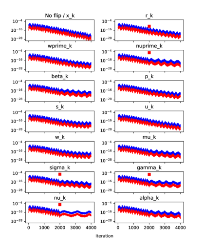
Figure 10: $\nu$-gap (red) and $\nu$-bound (blue) graph, matrix nos7

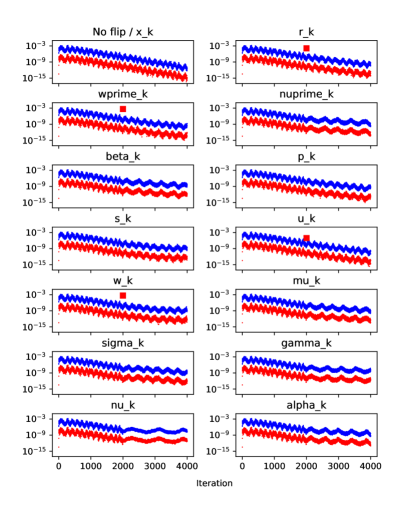
Figure 11: $\mathbf{w}$-gap (red) and $\mathbf{w}$-bound (blue) graph, matrix nos7

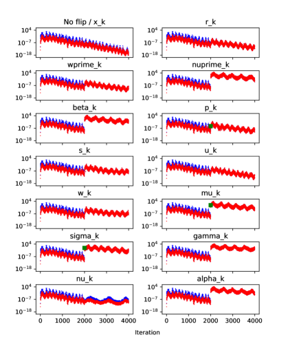
Figure 12: $\mu$-gap (red) and $\mu$-bound (blue) graph, matrix nos7

Appendix C Complete Detection Performance Experiments

Here we present the results of the detection experiment for each of the Pipe-PR-CG variables separately. Besides the categorization of runs into the six categories, as was done in Table 4, these tables also contain in the columns information about the lowest numbered bit for each matrix whose run was classified as special negative (snbit), so that the interesting aspect of an undetected bit flip which does not destroy convergence can be examined. On top of that, it is also noted what was the highest bit for which an overflow error occurred (ovbit). At the bottom of each variable table the extrema of the snbit and ovbit values over all matrices are presented.

matrix	threshold	tp	sp	fp	tn	sn	fn	snbit	ovbit
1138_bus	$5\mathrm{e}{-1}$	76	274	217	134	290	0	29	2
	$1\mathrm{e}{-4}$	88	354	0	200	349	0	29	2
bcsstm07	$5\mathrm{e}{-1}$	15	457	0	200	319	0	31	2
	$1\mathrm{e}{-4}$	15	453	0	200	323	0	31	2
bundle1	$5\mathrm{e}{-1}$	16	336	0	200	441	0	15	2
	$1\mathrm{e}{-4}$	16	333	0	200	444	0	15	2
wathen120	$5\mathrm{e}{-1}$	8	393	0	200	386	0	28	2
	$1\mathrm{e}{-4}$	8	393	0	200	386	0	28	2
bcsstk05	$5\mathrm{e}{-1}$	218	328	22	181	240	0	42	2
	$1\mathrm{e}{-4}$	218	318	0	200	253	0	42	2
gr_30_30	$5\mathrm{e}{-1}$	23	507	0	200	263	0	39	2
	$1\mathrm{e}{-4}$	23	507	0	200	263	0	39	2
nos7	$5\mathrm{e}{-1}$	0	0	985	0	0	0	-	2
	$1\mathrm{e}{-4}$	63	233	307	87	295	0	12	2
crystm01	$5\mathrm{e}{-1}$	11	417	0	200	361	0	32	2
	$1\mathrm{e}{-4}$	11	417	0	200	361	0	32	2
$\sum$ or extrema	$5\mathrm{e}{-1}$	367	2712	1224	1315	2300	0	15	2
	$1\mathrm{e}{-4}$	442	3008	307	1487	2674	0	12	2

Table 5: Detection performance, bit flip in $\mathbf{r_{k}}$

matrix	threshold	tp	sp	fp	tn	sn	fn	snbit	ovbit
1138_bus	$5\mathrm{e}{-1}$	102	233	199	123	327	1	27	5
	$1\mathrm{e}{-4}$	106	287	0	200	391	1	27	5
bcsstm07	$5\mathrm{e}{-1}$	30	459	0	200	299	1	33	4
	$1\mathrm{e}{-4}$	30	445	0	200	313	1	29	4
bundle1	$5\mathrm{e}{-1}$	38	294	0	200	435	0	24	9
	$1\mathrm{e}{-4}$	38	270	0	200	459	0	22	9
wathen120	$5\mathrm{e}{-1}$	7	428	0	200	353	1	30	9
	$1\mathrm{e}{-4}$	7	428	0	200	353	1	30	9
bcsstk05	$5\mathrm{e}{-1}$	225	330	27	183	211	0	42	5
	$1\mathrm{e}{-4}$	230	300	0	200	246	0	39	5
gr_30_30	$5\mathrm{e}{-1}$	38	472	0	200	272	0	40	4
	$1\mathrm{e}{-4}$	38	470	0	200	274	0	40	4
nos7	$5\mathrm{e}{-1}$	0	0	988	0	0	0	-	3
	$1\mathrm{e}{-4}$	66	173	304	85	360	0	1	3
crystm01	$5\mathrm{e}{-1}$	25	411	0	200	354	0	33	2
	$1\mathrm{e}{-4}$	25	411	0	200	354	0	33	2
$\sum$ or extrema	$5\mathrm{e}{-1}$	465	2627	1214	1306	2251	3	24	9
	$1\mathrm{e}{-4}$	540	2784	304	1485	2750	3	1	9

Table 6: Detection performance, bit flip in $\mathbf{w^{\prime}_{k}}$

matrix	threshold	tp	sp	fp	tn	sn	fn	snbit	ovbit
1138_bus	$5\mathrm{e}{-1}$	95	428	204	125	139	0	50	3
	$1\mathrm{e}{-4}$	106	513	0	200	172	0	49	3
bcsstm07	$5\mathrm{e}{-1}$	50	584	0	200	154	0	51	3
	$1\mathrm{e}{-4}$	50	569	0	200	169	0	51	3
bundle1	$5\mathrm{e}{-1}$	45	538	0	200	206	0	47	3
	$1\mathrm{e}{-4}$	45	518	0	200	226	0	46	3
wathen120	$5\mathrm{e}{-1}$	40	524	0	200	224	0	46	3
	$1\mathrm{e}{-4}$	40	506	0	200	242	0	45	3
bcsstk05	$5\mathrm{e}{-1}$	197	462	19	184	127	0	52	3
	$1\mathrm{e}{-4}$	197	448	0	200	144	0	51	3
gr_30_30	$5\mathrm{e}{-1}$	50	553	0	200	181	0	51	2
	$1\mathrm{e}{-4}$	50	529	0	200	205	0	50	2
nos7	$5\mathrm{e}{-1}$	0	0	988	0	0	0	-	3
	$1\mathrm{e}{-4}$	92	390	293	80	133	0	45	3
crystm01	$5\mathrm{e}{-1}$	46	550	0	200	192	0	49	2
	$1\mathrm{e}{-4}$	46	532	0	200	210	0	48	2
$\sum$ or extrema	$5\mathrm{e}{-1}$	523	3639	1211	1309	1223	0	46	3
	$1\mathrm{e}{-4}$	626	4005	293	1480	1501	0	45	3

Table 7: Detection performance, bit flip in $\nu^{\prime}_{k}$

matrix	threshold	tp	sp	fp	tn	sn	fn	snbit	ovbit
1138_bus	$5\mathrm{e}{-1}$	99	395	208	121	163	1	2	3
	$1\mathrm{e}{-4}$	112	289	0	200	385	1	2	3
bcsstm07	$5\mathrm{e}{-1}$	45	540	0	200	205	1	2	2
	$1\mathrm{e}{-4}$	45	364	0	200	381	1	2	2
bundle1	$5\mathrm{e}{-1}$	40	478	0	200	264	1	2	3
	$1\mathrm{e}{-4}$	40	310	0	200	432	1	2	3
wathen120	$5\mathrm{e}{-1}$	26	470	0	200	293	0	3	2
	$1\mathrm{e}{-4}$	26	297	0	200	466	0	3	2
bcsstk05	$5\mathrm{e}{-1}$	205	384	28	177	186	5	2	3
	$1\mathrm{e}{-4}$	200	240	0	200	335	10	2	3
gr_30_30	$5\mathrm{e}{-1}$	38	542	0	200	205	0	3	2
	$1\mathrm{e}{-4}$	38	379	0	200	368	0	3	2
nos7	$5\mathrm{e}{-1}$	0	0	989	0	0	0	-	3
	$1\mathrm{e}{-4}$	93	207	294	91	302	2	2	3
crystm01	$5\mathrm{e}{-1}$	18	511	0	200	262	0	3	2
	$1\mathrm{e}{-4}$	18	349	0	200	424	0	3	2
$\sum$ or extrema	$5\mathrm{e}{-1}$	471	3320	1225	1298	1578	8	2	3
	$1\mathrm{e}{-4}$	572	2435	294	1491	3093	15	2	3

Table 8: Detection performance, bit flip in $\beta_{k}$

matrix	threshold	tp	sp	fp	tn	sn	fn	snbit	ovbit
1138_bus	$5\mathrm{e}{-1}$	73	282	214	125	297	0	28	2
	$1\mathrm{e}{-4}$	79	337	0	200	375	0	27	2
bcsstm07	$5\mathrm{e}{-1}$	16	479	0	200	294	0	34	2
	$1\mathrm{e}{-4}$	16	460	0	200	313	0	30	2
bundle1	$5\mathrm{e}{-1}$	2	368	0	200	411	0	25	8
	$1\mathrm{e}{-4}$	2	347	0	200	432	0	19	8
wathen120	$5\mathrm{e}{-1}$	9	354	0	200	425	0	26	2
	$1\mathrm{e}{-4}$	9	342	0	200	437	0	23	2
bcsstk05	$5\mathrm{e}{-1}$	170	392	27	178	222	0	42	3
	$1\mathrm{e}{-4}$	170	374	0	200	245	0	39	3
gr_30_30	$5\mathrm{e}{-1}$	7	517	0	200	265	0	38	2
	$1\mathrm{e}{-4}$	7	497	0	200	285	0	36	2
nos7	$5\mathrm{e}{-1}$	0	0	986	0	0	0	-	3
	$1\mathrm{e}{-4}$	59	179	290	96	362	0	20	3
crystm01	$5\mathrm{e}{-1}$	4	420	0	200	365	0	32	2
	$1\mathrm{e}{-4}$	4	405	0	200	380	0	30	2
$\sum$ or extrema	$5\mathrm{e}{-1}$	281	2812	1227	1303	2279	0	25	8
	$1\mathrm{e}{-4}$	346	2941	290	1496	2829	0	19	8

Table 9: Detection performance, bit flip in $\mathbf{p_{k}}$

matrix	threshold	tp	sp	fp	tn	sn	fn	snbit	ovbit
1138_bus	$5\mathrm{e}{-1}$	144	212	215	131	279	0	31	4
	$1\mathrm{e}{-4}$	158	121	0	200	498	4	18	4
bcsstm07	$5\mathrm{e}{-1}$	27	453	0	200	300	1	29	4
	$1\mathrm{e}{-4}$	27	289	0	200	464	1	18	4
bundle1	$5\mathrm{e}{-1}$	35	308	0	200	426	0	26	8
	$1\mathrm{e}{-4}$	35	136	0	200	598	0	1	8
wathen120	$5\mathrm{e}{-1}$	3	354	0	200	427	0	24	9
	$1\mathrm{e}{-4}$	3	191	0	200	590	0	14	9
bcsstk05	$5\mathrm{e}{-1}$	241	326	30	173	212	0	43	4
	$1\mathrm{e}{-4}$	241	160	0	200	381	0	28	4
gr_30_30	$5\mathrm{e}{-1}$	22	477	0	200	293	0	40	3
	$1\mathrm{e}{-4}$	22	320	0	200	450	0	23	3
nos7	$5\mathrm{e}{-1}$	0	0	983	0	0	0	-	5
	$1\mathrm{e}{-4}$	106	56	274	106	439	2	4	5
crystm01	$5\mathrm{e}{-1}$	30	373	0	200	390	0	32	2
	$1\mathrm{e}{-4}$	30	202	0	200	561	0	19	2
$\sum$ or extrema	$5\mathrm{e}{-1}$	502	2503	1228	1304	2327	1	24	9
	$1\mathrm{e}{-4}$	622	1475	274	1506	3981	7	4	9

Table 10: Detection performance, bit flip in $\mathbf{s_{k}}$

matrix	threshold	tp	sp	fp	tn	sn	fn	snbit	ovbit
1138_bus	$5\mathrm{e}{-1}$	79	221	218	122	337	0	27	4
	$1\mathrm{e}{-4}$	87	279	0	200	411	0	26	4
bcsstm07	$5\mathrm{e}{-1}$	55	422	2	200	307	0	34	4
	$1\mathrm{e}{-4}$	56	414	0	200	316	0	34	4
bundle1	$5\mathrm{e}{-1}$	20	308	0	200	442	0	24	7
	$1\mathrm{e}{-4}$	20	292	0	200	458	0	18	7
wathen120	$5\mathrm{e}{-1}$	11	380	0	200	385	0	31	8
	$1\mathrm{e}{-4}$	11	380	0	200	385	0	31	8
bcsstk05	$5\mathrm{e}{-1}$	240	308	26	181	218	0	43	5
	$1\mathrm{e}{-4}$	241	292	0	200	240	0	40	5
gr_30_30	$5\mathrm{e}{-1}$	44	467	0	200	272	1	42	4
	$1\mathrm{e}{-4}$	44	466	0	200	273	1	40	4
nos7	$5\mathrm{e}{-1}$	0	0	978	0	0	0	-	4
	$1\mathrm{e}{-4}$	41	122	298	97	420	0	1	4
crystm01	$5\mathrm{e}{-1}$	37	422	0	200	335	0	31	2
	$1\mathrm{e}{-4}$	37	421	0	200	336	0	31	2
$\sum$ or extrema	$5\mathrm{e}{-1}$	486	2528	1224	1303	2296	1	24	8
	$1\mathrm{e}{-4}$	537	2666	298	1497	2839	1	1	8

Table 11: Detection performance, bit flip in $\mathbf{u_{k}}$

matrix	threshold	tp	sp	fp	tn	sn	fn	snbit	ovbit
1138_bus	$5\mathrm{e}{-1}$	88	274	202	130	297	0	29	3
	$1\mathrm{e}{-4}$	99	331	0	200	361	0	29	3
bcsstm07	$5\mathrm{e}{-1}$	29	472	0	200	289	0	31	4
	$1\mathrm{e}{-4}$	29	461	0	200	300	0	31	4
bundle1	$5\mathrm{e}{-1}$	39	289	0	200	430	0	23	9
	$1\mathrm{e}{-4}$	39	272	0	200	447	0	21	9
wathen120	$5\mathrm{e}{-1}$	3	385	0	200	393	0	29	9
	$1\mathrm{e}{-4}$	3	385	0	200	393	0	29	9
bcsstk05	$5\mathrm{e}{-1}$	245	298	33	174	219	0	44	4
	$1\mathrm{e}{-4}$	246	274	0	200	249	0	43	4
gr_30_30	$5\mathrm{e}{-1}$	39	485	0	200	271	0	39	4
	$1\mathrm{e}{-4}$	39	482	0	200	274	0	39	4
nos7	$5\mathrm{e}{-1}$	0	0	988	0	0	0	-	4
	$1\mathrm{e}{-4}$	70	181	294	96	347	0	6	4
crystm01	$5\mathrm{e}{-1}$	20	427	0	200	343	0	34	2
	$1\mathrm{e}{-4}$	20	427	0	200	343	0	34	2
$\sum$ or extrema	$5\mathrm{e}{-1}$	463	2630	1223	1304	2242	0	23	9
	$1\mathrm{e}{-4}$	545	2813	294	1496	2714	0	6	9

Table 12: Detection performance, bit flip in $\mathbf{w_{k}}$

matrix	threshold	tp	sp	fp	tn	sn	fn	snbit	ovbit
1138_bus	$5\mathrm{e}{-1}$	144	378	199	122	141	0	50	4
	$1\mathrm{e}{-4}$	173	430	0	200	181	0	49	4
bcsstm07	$5\mathrm{e}{-1}$	129	493	0	200	160	0	52	4
	$1\mathrm{e}{-4}$	129	479	0	200	174	0	50	4
bundle1	$5\mathrm{e}{-1}$	91	482	0	200	210	0	49	4
	$1\mathrm{e}{-4}$	91	470	0	200	222	0	48	4
wathen120	$5\mathrm{e}{-1}$	126	425	0	200	231	0	47	4
	$1\mathrm{e}{-4}$	126	416	0	200	240	0	46	4
bcsstk05	$5\mathrm{e}{-1}$	262	409	28	178	112	0	54	4
	$1\mathrm{e}{-4}$	265	394	0	200	130	0	52	4
gr_30_30	$5\mathrm{e}{-1}$	117	508	0	200	159	0	53	4
	$1\mathrm{e}{-4}$	117	496	0	200	171	0	52	4
nos7	$5\mathrm{e}{-1}$	0	0	986	0	0	0	-	4
	$1\mathrm{e}{-4}$	143	260	287	104	192	0	43	4
crystm01	$5\mathrm{e}{-1}$	110	519	0	200	160	0	51	3
	$1\mathrm{e}{-4}$	110	505	0	200	174	0	49	3
$\sum$ or extrema	$5\mathrm{e}{-1}$	979	3214	1213	1300	1173	0	47	4
	$1\mathrm{e}{-4}$	1154	3450	287	1504	1484	0	43	4

Table 13: Detection performance, bit flip in $\mu_{k}$

matrix	threshold	tp	sp	fp	tn	sn	fn	snbit	ovbit
1138_bus	$5\mathrm{e}{-1}$	162	361	206	127	133	0	50	3
	$1\mathrm{e}{-4}$	185	436	0	200	168	0	49	3
bcsstm07	$5\mathrm{e}{-1}$	118	502	0	200	167	0	52	3
	$1\mathrm{e}{-4}$	118	493	0	200	176	0	52	3
bundle1	$5\mathrm{e}{-1}$	141	462	0	200	192	0	49	3
	$1\mathrm{e}{-4}$	141	441	0	200	213	0	48	3
wathen120	$5\mathrm{e}{-1}$	134	427	0	200	228	0	47	3
	$1\mathrm{e}{-4}$	134	416	0	200	239	0	46	3
bcsstk05	$5\mathrm{e}{-1}$	250	409	27	180	119	0	53	3
	$1\mathrm{e}{-4}$	252	398	0	200	135	0	52	3
gr_30_30	$5\mathrm{e}{-1}$	178	472	0	200	130	1	53	3
	$1\mathrm{e}{-4}$	178	459	0	200	143	1	52	3
nos7	$5\mathrm{e}{-1}$	0	0	984	0	0	0	-	3
	$1\mathrm{e}{-4}$	144	332	295	100	113	0	47	3
crystm01	$5\mathrm{e}{-1}$	136	458	0	200	193	0	50	2
	$1\mathrm{e}{-4}$	136	438	0	200	213	0	49	2
$\sum$ or extrema	$5\mathrm{e}{-1}$	1119	3091	1217	1307	1162	1	47	3
	$1\mathrm{e}{-4}$	1288	3413	295	1500	1400	1	46	3

Table 14: Detection performance, bit flip in $\sigma_{k}$

matrix	threshold	tp	sp	fp	tn	sn	fn	snbit	ovbit
1138_bus	$5\mathrm{e}{-1}$	169	372	210	128	114	0	51	3
	$1\mathrm{e}{-4}$	195	445	0	200	153	0	51	3
bcsstm07	$5\mathrm{e}{-1}$	139	515	0	200	140	0	52	3
	$1\mathrm{e}{-4}$	139	498	0	200	157	0	52	3
bundle1	$5\mathrm{e}{-1}$	132	459	0	200	195	0	48	3
	$1\mathrm{e}{-4}$	132	444	0	200	210	0	48	3
wathen120	$5\mathrm{e}{-1}$	128	428	0	200	233	0	47	3
	$1\mathrm{e}{-4}$	128	418	0	200	243	0	46	3
bcsstk05	$5\mathrm{e}{-1}$	248	408	34	177	121	0	54	3
	$1\mathrm{e}{-4}$	249	406	0	200	133	0	54	3
gr_30_30	$5\mathrm{e}{-1}$	153	507	0	200	124	0	53	3
	$1\mathrm{e}{-4}$	153	483	0	200	148	0	51	3
nos7	$5\mathrm{e}{-1}$	0	0	983	0	0	0	-	3
	$1\mathrm{e}{-4}$	165	307	313	100	98	0	51	3
crystm01	$5\mathrm{e}{-1}$	125	497	0	200	163	0	50	2
	$1\mathrm{e}{-4}$	125	473	0	200	187	0	49	2
$\sum$ or extrema	$5\mathrm{e}{-1}$	1094	3186	1227	1305	1090	0	47	3
	$1\mathrm{e}{-4}$	1286	3474	313	1500	1329	0	46	3

Table 15: Detection performance, bit flip in $\gamma_{k}$

matrix	threshold	tp	sp	fp	tn	sn	fn	snbit	ovbit
1138_bus	$5\mathrm{e}{-1}$	155	333	197	130	170	0	50	3
	$1\mathrm{e}{-4}$	181	410	0	200	194	0	49	3
bcsstm07	$5\mathrm{e}{-1}$	174	462	0	200	152	0	51	3
	$1\mathrm{e}{-4}$	174	462	0	200	152	0	51	3
bundle1	$5\mathrm{e}{-1}$	139	413	0	200	228	0	46	3
	$1\mathrm{e}{-4}$	139	413	0	200	228	0	46	3
wathen120	$5\mathrm{e}{-1}$	143	393	0	200	249	1	45	4
	$1\mathrm{e}{-4}$	143	393	0	200	249	1	45	4
bcsstk05	$5\mathrm{e}{-1}$	261	361	29	175	157	0	52	3
	$1\mathrm{e}{-4}$	261	361	0	200	161	0	52	3
gr_30_30	$5\mathrm{e}{-1}$	144	479	0	200	165	0	51	3
	$1\mathrm{e}{-4}$	144	479	0	200	165	0	51	3
nos7	$5\mathrm{e}{-1}$	0	0	983	0	0	0	-	3
	$1\mathrm{e}{-4}$	178	285	299	96	135	0	48	2
crystm01	$5\mathrm{e}{-1}$	142	423	0	200	223	1	48	3
	$1\mathrm{e}{-4}$	142	423	0	200	223	1	48	3
$\sum$ or extrema	$5\mathrm{e}{-1}$	1158	2864	1219	1305	1344	2	45	4
	$1\mathrm{e}{-4}$	1362	3226	299	1496	1507	2	45	4

Table 16: Detection performance, bit flip in $\nu_{k}$

matrix	threshold	tp	sp	fp	tn	sn	fn	snbit	ovbit
1138_bus	$5\mathrm{e}{-1}$	146	362	192	134	157	0	46	2
	$1\mathrm{e}{-4}$	163	277	0	200	351	0	31	2
bcsstm07	$5\mathrm{e}{-1}$	112	504	0	200	174	0	44	2
	$1\mathrm{e}{-4}$	112	323	0	200	355	0	34	2
bundle1	$5\mathrm{e}{-1}$	95	478	0	200	208	0	44	2
	$1\mathrm{e}{-4}$	95	308	0	200	378	0	31	2
wathen120	$5\mathrm{e}{-1}$	133	370	0	200	286	0	41	2
	$1\mathrm{e}{-4}$	133	204	0	200	452	0	27	2
bcsstk05	$5\mathrm{e}{-1}$	229	378	18	183	170	0	49	2
	$1\mathrm{e}{-4}$	229	221	0	200	328	0	33	2
gr_30_30	$5\mathrm{e}{-1}$	111	493	0	200	183	0	50	2
	$1\mathrm{e}{-4}$	111	333	0	200	343	0	36	2
nos7	$5\mathrm{e}{-1}$	0	0	992	0	0	0	-	2
	$1\mathrm{e}{-4}$	161	156	295	91	289	0	27	2
crystm01	$5\mathrm{e}{-1}$	95	468	0	200	223	0	47	4
	$1\mathrm{e}{-4}$	95	289	0	200	402	0	33	4
$\sum$ or extrema	$5\mathrm{e}{-1}$	921	3053	1202	1317	1401	0	41	4
	$1\mathrm{e}{-4}$	1099	2111	295	1491	2898	0	27	4

Table 17: Detection performance, bit flip in $\alpha_{k}$

References

- [1] Emmanuel Agullo, Siegfried Cools, Luc Giraud, Alexandre Moreau, Pablo Salas, Wim Vanroose, Emrullah Fatih Yetkin, and Mawussi Zounon. Hard faults and soft-errors: possible numerical remedies in linear algebra solvers. In High Performance Computing for Computational Science–VECPAR 2016: 12th International Conference, Porto, Portugal, June 28-30, 2016, Revised Selected Papers 12, pages 11–18. Springer, 2017.
- [2] Emmanuel Agullo, Siegfried Cools, Emrullah Fatih Yetkin, Luc Giraud, Nick Schenkels, and Wim Vanroose. On soft errors in the conjugate gradient method: Sensitivity and robust numerical detection. SIAM Journal on Scientific Computing, 42(6):C336–C358, 2020.
- [3] Guillaume Aupy, Anne Benoit, Aurlien Cavelan, Massimiliano Fasi, Yves Robert, Hongyang Sun, and Bora Uçar. Coping with Silent Errors in HPC Applications, pages 269–292. Springer International Publishing, Cham, 2017.
- [4] Greg Bronevetsky and Bronis de Supinski. Soft error vulnerability of iterative linear algebra methods. In Proceedings of the 22nd Annual International Conference on Supercomputing, pages 155–164, 2008.
- [5] Erin Carson, Miroslav Rozložník, Zdeněk Strakoš, Petr Tichý, and Miroslav Tůma. The numerical stability analysis of pipelined conjugate gradient methods: Historical context and methodology. SIAM Journal on Scientific Computing, 40(5):A3549–A3580, 2018.
- [6] Tyler Chen and Erin Carson. Predict-and-recompute conjugate gradient variants. SIAM Journal on Scientific Computing, 42(5):A3084–A3108, 2020.
- [7] A.T. Chronopoulos and C.W. Gear. s-step iterative methods for symmetric linear systems. Journal of Computational and Applied Mathematics, 25(2):153–168, 1989.
- [8] Timothy A. Davis and Yifan Hu. The University of Florida sparse matrix collection. ACM Trans. Math. Softw., 38(1), dec 2011.
- [9] James Elliott, Mark Hoemmen, and Frank Mueller. Evaluating the impact of SDC on the GMRES iterative solver. pages 1193–1202, 2014.
- [10] James Elliott, Mark Hoemmen, and Frank Mueller. A numerical soft fault model for iterative linear solvers. In Proceedings of the 24th International Symposium on High-Performance Parallel and Distributed Computing, pages 271–274, 2015.
- [11] P. Ghysels and W. Vanroose. Hiding global synchronization latency in the preconditioned conjugate gradient algorithm. Parallel Computing, 40(7):224–238, 2014.
- [12] Scott Griffiths. Python module bitstring. (Version 4.1).
- [13] M. R. Hestenes and E. Stiefel. Methods of conjugate gradients for solving linear systems. Journal of Research of the National Bureau of Standards, 49(6), 1952.
- [14] G. Meurant. Detection and correction of silent errors in the conjugate gradient algorithm. Numerical Algorithms, 92:869–891, 2023.
- [15] G. Meurant and P. Tichý. Approximating the extreme Ritz values and upper bounds for the A-norm of the error in CG. Numerical Algorithms, 82:937–968, 2019.
- [16] Gérard Meurant. Multitasking the conjugate gradient method on the CRAY X-MP/48. Parallel Computing, 5:267–280, 1987.
- [17] The University of Florida. SuiteSparse matrix collection. https://sparse.tamu.edu (Last accessed on 2023/11/25).