Symbolic State Partitioning for
Reinforcement Learning

Abstract

Tabular reinforcement learning methods cannot operate directly on continuous state spaces. One solution for this problem is to partition the state space. A good partitioning enables generalization during learning and more efficient exploitation of prior experiences. Consequently, the learning process becomes faster and produces more reliable policies. However, partitioning introduces approximation, which is particularly harmful in the presence of nonlinear relations between state components. An ideal partition should be as coarse as possible, while capturing the key structure of the state space for the given problem. This work extracts partitions from the environment dynamics by symbolic execution. We show that symbolic partitioning improves state space coverage with respect to environmental behavior and allows reinforcement learning to perform better for sparse rewards. We evaluate symbolic state space partitioning with respect to precision, scalability, learning agent performance and state space coverage for the learnt policies.

1 Introduction

Reinforcement learning is a form of active learning, where an agent learns to make decisions to maximize a reward signal. The agent interacts with an environment and takes actions based on its current state. The environment rewards the agent, which uses the reward value to update its decision-making policy. Reinforcement learning has applications in many domains: robotics [1], gaming [2], electronic [3], healthcare [4]. This method can automatically synthesize controllers for many challenging control problems [5], however dedicated approximation techniques, hereunder deep learning, are needed for continuous state spaces. Unfortunately, despite many spectacular success with continuous problems, Deep Reinforcement Learning suffers from low explainability and lack of convergence guarantees. At the same time discrete (tabular) learning methods have been shown to be more explainable [6, 7, 8, 9] and to yield policies for which it is easier to assure safety [10, 11, 12]; for instance using formal verification [13, 14, 15]. Thus, finding a good state-space representation for discrete learning remains an active research area [16, 17, 18] [19, 20, 21, 22].

To adapt a continuous state space for discrete learning, one exploits partial observability, and merges regions of the state space into discrete partitions, each representing a subset of the states of the agent. Ideally, all states in a partition should capture meaningful aspects of the environment—best if they ensure the Markov property for the environment dynamics. Consequently, a good partitioning depends on the problem at hand. For instance, in safety critical environments, it is essential to identify small “singularities”—regions that require special handling—even if they are very small. Otherwise, if such regions are included in larger partitions, the control policy will not be able to distinguish them from the surrounding, leading to high variance at operation time and slow convergence of learning.

The trade-off between the size of the partitioning and the optimality and convergence of reinforcement learning remains a challenge [17, 18, 19, 20, 21, 22]. Policies obtained for coarse-grained partitionings are unreliable. Large fine-grained partitionings make reinforcement learning slow. The dominant methods are tiling and vector quantization [17, 18, 20, 21]; both are not adaptive to the structure of the state space. They ignore nonlinear dependencies between state components even though quadratic behaviors are common in control systems. So far, the shape of the state partitions has hardly been studied.

In this work, we investigate the use of symbolic execution to extract approximate adaptive partitionings that reflect the problem dynamics. Symbolic execution is a classic and established program analysis technique [23, 24], commonly used in testing and verification. A symbolic executor generates a set of path conditions ($\mathit{PC}$), constraints that must hold for each execution path of the program to be taken. These conditions partition the state space of the executed program into groups that share the same execution path. Our hypothesis is that the path conditions obtained by symbolic execution of an environment model (the step and reward functions) provide a useful state space partition for reinforcement learning. The branches in the environment program likely reflect important aspects of the problem dynamics that should be respected by an optimal policy. We test this hypothesis by:

• Defining a symbolic partitioning method and establishing its basic theoretical properties. This method, SymPar, is adaptive to the problem semantics, general (not developed for a specific problem), and automatic (given a symbolically executable environment program).

• Implementing the method on top of the Symbolic PathFinder, an established symbolic executor for Java programs (JVM programs) [25]

• Evaluating SymPar empirically against other offline and online partitioning approaches, and against deep reinforcement learning methods. The experiments show that symbolic partitioning can allow the agent to learn better policies than with the baselines.

To the best of our knowledge, this is the first ever attempt to use symbolic execution to breath semantic knowledge into an otherwise statistical reinforcement learning process. It brakes with the tradition of reinforcement learning to treat environments as black-boxes. It is however consistent with common practice of using reinforcement learning for software defined problems and with pre-training robotic agents in simulators, as software problems and simulators are amenable to symbolic execution.

Related Work

We study partitioning of the state space in reinforcement learning by mapping from a continuous state space to a discrete one or by aggregating discrete states. The earliest use of partitioning, to the best of our knowledge, was the BOXES systems [26]. The Parti-game algorithm [27] automatically partitions state spaces but applies only to tasks with known goal regions and requires a greedy local controller. While tile coding is a classic method for partitioning [28], it often demands extensive engineering efforts to avoid misleading the agent with suboptimal partitions. [29] extended learning classifier systems to use tile coding. Techniques such as vector quantization [17, 18, 20, 21] and decision trees [30, 31, 32] lack adaptability to the properties of the state space and may overlook non-linear dependencies among state components. Techniques that gradually refine a coarse partitioning during the learning process [16, 18, 19, 20, 22] are time-intensive, and require generating numerous partitions to achieve better approximations near the boundaries of nonlinear functions.

Unlike other methods, SymPar incurs no learning costs (offline), requires no engineering effort (automated), and is not problem specific in contrast to some of the existing techniques (general). It produces a partitioning that effectively captures non-linear dependencies as well as narrow partitions, without incurring additional costs or increasing the number of partitions at the boundaries.

2 Background

Reinforcement Learning.

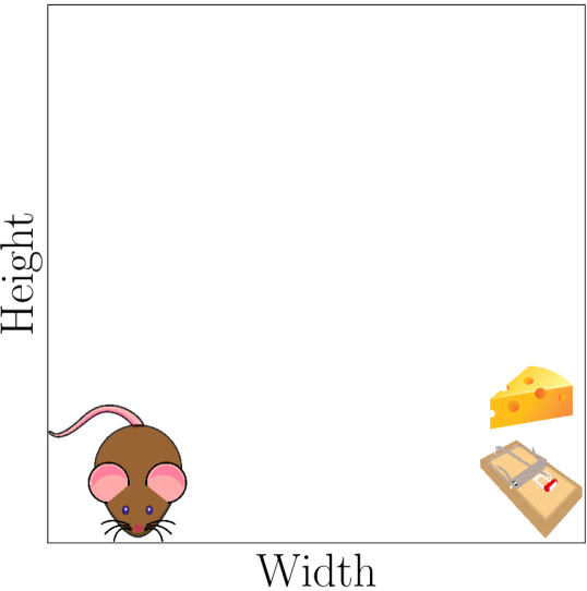
Figure 1: Navigation environment.

A Partially Observable Markov Decision Process is a tuple $\mathcal{M}=(\overline{\mathcal{S}},\overline{\mathcal{S}}_{0},\linebreak[3]\mathcal{A},\mathcal{S},\linebreak[2]\mathcal{O},\mathcal{T}\!,\mathcal{R},\mathcal{F})$, where $\overline{\mathcal{S}}$ is a set of states, $\overline{\mathcal{S}}_{0}\in\textnormal{pdf }\overline{\mathcal{S}}$ is a probability density function for initial states, $\mathcal{A}$ is a finite set of actions, $\mathcal{S}$ is a finite set of observable states, $\mathcal{O}\in\overline{\mathcal{S}}\to\mathcal{S}$ is a total observation function, $\mathcal{T}\in\overline{\mathcal{S}}\times\mathcal{A}\to\textnormal{pdf }\overline{\mathcal{S}}$ is the transition probability function, $\mathcal{R}\in\overline{\mathcal{S}}\times\mathcal{A}\to\mathbb{R}$ is the reward function, and $\mathcal{F}\in\mathcal{S}\to\{0,1\}$ is a predicate defining final states. The task is to find a policy $\pi:\mathcal{S}\to\text{Dist}(\mathcal{A})$ that maximizes the expected accumulated reward [5].

Example 1.

Consider a room with dimensions $W\!\times\!H$, a mouse in its bottom-left corner, a mousetrap in the bottom-right corner, and a piece of cheese next to the mousetrap (Fig. 1). The mouse moves with a fixed velocity in four directions: up, down, left, right. Its goal is to find the cheese but avoid the trap. The states $\overline{\mathcal{S}}$ are ordered pairs representing the mouse’s position in the room. The set of initial states $\overline{\mathcal{S}}_{0}$ is fixed to $(1,1)$, a Dirac distribution. We define the actions as the set of all possible movements for the mouse: $\mathcal{A}$ $=\{(d,v):d\in\mathcal{D},v\in\mathcal{V}\}$, where $\mathcal{D}=\{U,D,R,L\}$ and $\mathcal{V}=\{r_{1},r_{2},\dots,r_{n}\ |\ r_{i}\in\mathbb{R}^{+}\}$. $\mathcal{S}$ can be any partitioning of the room space and $\mathcal{O}$ is the map from the real position of the mouse to the partition containing it. Our goal is to find the partitioning, i.e., $\mathcal{S}$ and $\mathcal{O}$. The reward function $\mathcal{R}$ is zero when mouse finds the cheese, and $-1$ otherwise. For simplicity, we let the environment be deterministic, so $\mathcal{T}$ is a deterministic movement of the mouse from a position by a given action to a new position. The final state predicate $\mathcal{F}$ holds for the cheese and trap positions and not otherwise.

Symbolic Execution

is a program analysis technique that systematically explores program behaviors by solving symbolic constraints obtained from conjoining the program’s branch conditions [23]. Symbolic execution extends normal execution by running the basic operators of a language using symbolic inputs (variables) and producing symbolic formulas as output. A symbolic execution of a program produces a set of path conditions—logical expressions that encode conditions on the input symbols to follow a particular path in the program.

For a program over input arguments $I=\{v_{1},v_{2},\dots,v_{k}\}$, a path condition $\phi\in\mathit{PC}(I^{\prime})$ is a quantifier free logical formula defined on $I^{\prime}=\{\vartheta_{1},\vartheta_{2},\dots,\vartheta_{k}\}$, where each symbolic variable $\vartheta_{i}$ corresponds to $v_{i}$.

We sketch a definition of symbolic execution for a minimal language. [33] provide more details. Let $V$ be the set of program variables and Ops be a set of arithmetic operations, $x\in V$, $n\in\mathbb{R}$, and $op\in\textrm{Ops}$. We consider programs generated by the following grammar:

$$e::=x\ |\ n\ |\ op(e_{1},\dots,e_{n})$$ (1)

$$b::=\textrm{True}\ |\ \textrm{False}\ |\ b_{1}\text{ AND }b_{2}\ |\ b_{1}\text{ OR }b_{2}\ |\ \neg b\ |\ b_{1}\leq b_{2}\ |\ e_{1}<e_{2}$$

$$s::=x:=e\ |\ x\sim\textrm{rnd}\ |\ s_{1};s_{2}\ |\ \text{if }b\ s_{1}\ \text{else }s_{2}\ |\ \text{while }b\ s\ |\ \text{skip}$$

A symbolic store, denoted by $\sigma$ maps input program variables $I\subseteq V$ to expressions, generated by productions $e$ above. An update to a symbolic store is denoted $\sigma[x:=e]$. It replaces the entry for variable $x$ with the expression $e$. An expression can be interpreted in a symbolic store by applying (substituting) its mapping to the expression syntax (written $e\sigma$).

S-ASSIGN $$(x:=e,\sigma,k,\phi) ~{}~{}\rightarrow~{}~{}(\text{skip},\sigma[x\mapsto\sigma e],k,\phi)$$

S-IF-T $$(\text{if }b\ s_{1}\ \text{else }\ s_{2},\sigma,k,\phi) ~{}~{}\rightarrow~{}~{}(s_{1},\sigma,k,\phi\wedge\ \sigma b)$$

S-IF-F $$(\text{if }b\ s_{1}\ \text{else }\ s_{2},\sigma,k,\phi) ~{}~{}\rightarrow~{}~{}(s_{2},\sigma,k,\phi\wedge\ \sigma\neg b)$$

S-WHILE-T $$(\text{while }b\ s,\sigma,k,\phi) ~{}~{}\rightarrow~{}~{}(s\ ;\ \text{while }b\ s,\sigma,k,\phi\wedge\ \sigma b)$$

S-WHILE-F $$(\text{while }b\ s,\sigma,k,\phi) ~{}~{}\rightarrow~{}~{}(\text{skip}\ ;\ \sigma,k,\phi\wedge\ \sigma\neg b)$$

S-SMLP $$(x\sim\textrm{rnd},\sigma,k,\phi) ~{}~{}\rightarrow~{}~{}(\text{skip},\sigma[x\mapsto y_{k}],k+1,\phi)$$

Figure 2: Symbolic execution rules for an idealized probabilistic language. Each judgement is a quadruple: the program, the symbolic store ($\sigma$), the sample index ($k$), the current path condition ($\phi$).

Figure 2 gives the symbolic execution rules for the above language, in terms of traces (it computes a path condition $\phi$ for a terminating trace). In the reduction rules, $\phi$ represents the path condition and $k$ denotes the sampling index. The first rule defines the symbolic assignment; An assignment does not change the path conditions, but updates the symbolic store $\sigma$. When encountering conditional statements, the symbolic executor splits into two branches. For the true case (rule S-IF-T) the path condition is extended with the head condition of the branch, for the false case (S-IF-F), the path condition is extended with the negation of the branch condition. Similarly, for a while loop two branches are generated, with an analogous effect on path conditions. The last rule executes the randomized sampling statement. It simply allocates a new symbolic variable $y_{k}$ for the unknown result of sampling, and advances the sampling index [34]. Figure 3 (b) shows the path conditions obtained by applying similar rules to above for the code on the left hand side of the figure. The first path condition $PC^{(U,1)}$, corresponds to the branch where condition d==1 is true in the program.

The above rules can be used to prove basic properties of the symbolic execution. For example, as each path condition contains conjunction of different branch conditions in a program, the path conditions of the same program are mutually exclusive [33].

There exist practical symbolic executors for full scale programming languages. Even though we defined the concept at the level of syntax, the two most popular symbolic executors operate on compiled bytecode [25, 35]. In presence of loops and recursion, symbolic execution does not terminate. To halt symbolic execution, we can set a predefined timeout, an iteration limit, or a program statement limit. This produces an approximation of the set of path conditions.

3 Partitioning Using Symbolic Execution

⬇

W = 10 # Width

H = 10 # Height

def step(x, y, d, v):

if d == 1: # UP

if y < H:

return x, y+v

if d == 2: # DOWN

if y > 1:

return x, y-v

if d == 3: # LEFT

if x > 1:

return x-v, y

if d == 4: # RIGHT

if x < W:

return x+v, y

return x, y

def reward(x, y, d, v):

if x == W:

if y == 2:

return 0.0 # Cheese

elif y == 1:

return -1000.0 # Mousetrap

return -1.0

(a) The environment program

$\mathit{PC}^{(U,1)}$	$y<10\ \land x=10\ \land y+1=2$
	$y<10\ \land x=10\ \land y+1\neq 2$
	$y<10\ \land x\neq 10$
	$y\geq 10\ \land x=10$
	$y\geq 10\ \land x\neq 10$
$\mathit{PC}^{(D,1)}$	$y>1\ \land x=10\ \land y-1=2$
	$y>1\ \land x=10\ \land y-1\neq 2\ \wedge y-1=1$
	$y>1\ \land x=10\ \land y-1\neq 2\ \wedge y-1\neq 1$
	$y>1\ \land x\neq 10$
	$y\leq 1\ \land x=10\ \land y=1$
	$y\leq 1\ \land x\neq 10$
$\mathit{PC}^{(L,1)}$	$x>1\ \land x-1\neq 10$
	$x\leq 1\ \land x\neq 10$
$\mathit{PC}^{(R,1)}$	$x<10\ \land x+1=10\ \land y=2$
	$x<10\ \land x+1=10\ \land y\neq 2\ \land y=1$
	$x<10\ \land x+1=10\ \land y\neq 2\ \land y\neq 1$
	$x<10\ \land x+1\neq 10$
	$x\geq 10\ \land x=10\ \land y=2$
	$x\geq 10\ \land x=10\ \land y\neq 2\ \land y=1$
	$x\geq 10\ \land x=10\ \land y\neq 1\ \land y\neq 1$

(b) Path conditions collected by symbolic execution

Figure 3: The environment program for the navigation problem (Fig. 1)

We present the idea using a single agent with the environment modeled as a computer program. The program ($\mathit{Env}$) is implementing a single step-transition ($\mathcal{T}$) in the environment with the corresponding reward ($\mathcal{R}$). We use symbolic execution to analyze the environment program $\mathit{Env}$, then partition the state space using the obtained path conditions. The partitioning serves as the observation function $\mathcal{O}$. The entire process is automatic and generic—we follow the same procedure for all problems.

Example 2.

Figure 3(a) shows the environment program for the $10\times 10$ navigation problem (Example 1). For simplicity, we assume the agent can move one unit in each direction, so $\mathcal{V}=\{1\}$ and $\mathcal{A}=\{U,D,R,L\}\times\mathcal{V}$. The path conditions in Fig. 3(b) are obtained by symbolically executing the step and reward functions using symbolic inputs $x$ and $y$ and a concrete input from $\mathcal{A}$. Using path conditions in partitioning requires a translation from the symbolic executor syntax into the programming language used for implementing partitioning, as the executor will generate abstract value names.

A good partitioning maintains the Markov property, so that the same action is optimal for all unobservable states abstracted by the same partition. Unfortunately, this means that a good partitioning can be selected only once we know a good policy—after learning. To overcome this, SymPar heuristically bundles states into the same partition if they induce the same execution path in the environment program. We use an off-the-shelf symbolic executor to extract all possible path conditions from $\mathit{Env}$, by using $\overline{\mathcal{S}}$ as symbolic input and actions from $\mathcal{A}$ as concrete input. The result is a set $\mathit{PC}$ of path conditions for each concrete action: $\mathit{PC}=\{\mathit{PC}^{a_{0}},\mathit{PC}^{a_{1}},\dots,\mathit{PC}^{a_{m}}\}$, where $\mathit{PC}^{a}=\{\mathit{PC}^{a}_{0},\mathit{PC}^{a}_{1},\dots,\mathit{PC}^{a}_{k_{a}}\}$. The set $\mathit{PC}^{a}$ contains the path conditions computed for action $a$, and $k_{a}$ is the number of all path conditions obtained by running $\mathit{Env}$ symbolically, for a concrete action $a$.

Running the environment program for any concrete state satisfying a condition $\mathit{PC}^{a}_{i}$ with action $a$ will execute the same program path. However, the partitioning for reinforcement learning needs to be action independent (the same for all actions). So the path conditions cannot be used as partitions, as they are. Consider $\mathit{PC}_{i}^{a_{1}}\in\mathit{PC}^{a_{1}}$ and $\mathit{PC}_{j}^{a_{2}}\in\mathit{PC}^{a_{2}}$, arbitrary path conditions for some actions $a_{1}$, $a_{2}$. To make sure that the same program path will be taken from a concrete state for both actions, we need to create a partition that corresponds to the intersection of both path conditions: $\mathit{PC}_{i}^{a_{1}}\land\mathit{PC}_{j}^{a_{2}}$. In general, each set in $\mathit{PC}$ defines a partitioning of the state space for a different actions. To make them compatible, we need to compute the unique coarsest partitioning finer than those induced by the path conditions for any action, which is a standard operation in order theory [36]. In this case, this amounts to computing all intersections of partitions for all actions, and removing the empty intersections using an SMT check.

Figure 4: Overview of SymPar.

Figure 5: Using tile coding (left) and SymPar (right) for $10\!\times\!10$ and $50\!\times\!50$ navigation

The process of symbolic state space partitioning is summarized in figures 5 and 1. SymPar executes the environment program symbolically. For each action, a set of path conditions is collected. In the figure, $|\mathcal{A}|=5$ and, accordingly, five sets of path conditions are collected (shown as rectangles). Each rectangle is divided into a group of regions, each of which maps to a path condition. Thus, the rectangles illustrate the state space that is discretized by the path conditions. Note that the border of each region can be a unique path condition (an expression with equality relation) or a part of neighbour regions (an expression with inequality relation). The final partitioning is shown as another rectangle that contains the overlap between the regions from the previous step.

Example 3.

Figure 5 (left) shows the partitioning of the Navigation problem using tile coding [28] for two room sizes. Numerous cells share the same policy, prompting the question of why they should be divided. SymPar achieves a much coarser partitioning than the initial tiling, by discovering that for many tiles the dynamics is the same (right).

We handle stochasticity of the environment by allowing environment programs to be probabilistic and then following rule S-SMLP in symbolic execution (Fig. 2). We introduce a new symbolic variable whenever a random variable is sampled in the program [34, 37]. Consequently, our path conditions also contain these sampling variables. To make the process more reliable, one can generate constraints, limiting them to the support of the distribution. For example, for sampling from a uniform distribution $U[\alpha,\beta]$, the sampling variable $n_{v}$ is subject to two constraints: $n_{v}\!\geq\!\alpha$ and $n_{v}\!\leq\!\beta$. In order to be able to compute the partitioning over state variables only, as above, we existentially quantify the sampling variables out. This may introduce overlaps between the conditions, so we compute their intersection at this stage before proceeding.

Since the entire setup uses logical representations and an SMT solver, we exploit it further to generate witnesses for all partitions, even the smallest ones. We use them to seed reinforcement learning episodes, ensuring that each partition has been visited at least once. Consequently the agent is certain to learn from all the paths in the environment program. This can be further improved by constraining with a reachability predicate (not used in our examples).

Algorithm 1 Partitioning with Symbolic Execution (SymPar)

Input: $\mathit{Env}$, $\mathcal{A}$    Output: $\mathcal{P}$ (a partitioning of $\overline{\mathcal{S}}$)

1:$\mathit{PC}\leftarrow\emptyset$

2:for $a\in{}$$\mathcal{A}$ do

3:     $\mathit{PC}^{a},\Psi\leftarrow$ SymExec ($\mathit{Env}$, symbolic $\overline{\mathcal{S}}$, concrete $a$)    // $\Psi$ is the set of sampling variables

4:     Add distribution support constraints for all variables $\overline{\mathcal{S}}\in\Psi$ to $\mathit{PC}^{a}$

5:     Existentially quantify all sampling variables in $\mathit{PC}^{a}$     // may introduce overlaps of conditions

6:     $\mathit{PC}^{\prime a}\leftarrow\emptyset$

7:     for $p,q\in\mathit{PC}^{a}$ do if $\textbf{SAT}\ (p\wedge q)$ $PC^{\prime a}\leftarrow PC^{\prime a}\cup\{p\land q\}$      

8:     $\mathit{PC}^{a}\leftarrow PC^{\prime a}$

9:$\mathcal{P}\leftarrow\mathit{PC}^{\mathcal{A}[0]}$

10:for $a\in\mathcal{A}-\{\mathcal{A}[0]\}$ do

11:     $\mathcal{P}^{\prime}\leftarrow\emptyset$

12:     for $p\in\mathcal{P},q\in\mathit{PC}^{a}$ do if $\textbf{SAT}\ (p\wedge q)$ then $\mathcal{P}^{\prime}\leftarrow\mathcal{P}^{\prime}\cup\{p\land q\}$      

13:     $\mathcal{P}\leftarrow\mathcal{P}^{\prime}$

14:return $\mathcal{P}$

Properties of SymPar.

SymPar on the specifics of the environment implementation. Distinct implementations of the simulated environment may result in different partitioning outcomes for a given problem. On the other hand, the outcome is independent of the size of state space. Recall that in Fig. 5 (right) the number of partitionings is the same for the small and the large room.

To argue for the totality of our partitions, we first need to discuss completeness of the symbolic execution. De Boer and Bonsangue prove that symbolic execution is complete [33]. This result allows us to state the following theorem:

Theorem 1.

The obtained partitioning $\mathcal{P}$ is total for loop-free programs: $\forall\overline{s}\in\overline{\mathcal{S}}\;\exists!\,\mathcal{P}_{0}\in\mathcal{P}\cdot\;\overline{s}\in\mathcal{P}_{0}.$

In practice, symbolic execution is not complete, as most interesting programs with loops have infinitely many symbolic paths. This is easily overcome, by adding an extra path conditions, the complement of the computed ones, to cover for the unexplored paths.

The cost of SymPar amounts to exploring all paths in the program symbolically and then computing the coarsest partitioning. The symbolic execution involves generating a number of paths exponential in the number of branch points in the program (and at each branch one needs to solve an SMT problem—which is in principle undecidable, but works well for many practical problems). A practical approach is to bound the depth of exploration of paths by symbolic executor for more complex programs. Computing the coarsest partitioning requires solving $|\mathcal{P}|^{|\mathcal{A}|}$ number of SMT problems where $|\mathcal{P}|$ is the upper bound on the number of partitions (symbolic paths) and $|\mathcal{A}|$ is the number of actions. The other operations involved in this process such as computing and storing the path conditions in the required syntax are polynomial and efficient in practice.

Theorem 2.

Let $\mathit{PC}^{a}$ be the set of path conditions produced by SymPar for each of the actions $a\in\mathcal{A}$. The size of the final partitioning $\mathcal{P}$ returned by SymPar is bounded from below by each $|\mathit{PC}^{a}|$ and from above by $\prod_{a\in\mathcal{A}}|\mathit{PC}^{a}|$.

Note that SymPar is a heuristic and approximate method. To appreciate this, define the optimal partitioning to be the unique partitioning in which each partition contains all states with the same action in the optimal policy (the optimal partition is an inverse image of the optimal policy for all actions). The partitionings produced by SymPar are neither always coarser or always finer than the optimal one. This can be shown with simple counterexamples. For an environment with only one action, the optimal partitioning has only one partition as the optimal policy maps the same action for all states. But Sympar will generate more than one partition (a finer partitioning) if the simulation program contains branching. For problems without branching in the simulator such as cart pole problem, Sympar produces only one partition. However, the optimal partitioning contains more than one partition as optimal actions for all states in the state space are not the same. To understand the significance of this approximation in practice, we evaluate SymPar empirically against the existing methods.

4 Evaluation Setup

The partitioning of the state space faces a trade-off: on one hand, the granularity of the partitioning should be fine enough to distinguish crucial differences between states in the state space. On the other hand, this granularity should be chosen to avoid a combinatorial explosion, where the number of possible partitions becomes unmanageably large. Achieving this balance is essential for efficient and effective learning. In this section, we explore this trade-off and evaluate the performance of our implementation in SymPar empirically. To this aim, we address the following research questions:

RQ1  To what extent does SymPar produce smaller partitionings than other methods and how do RQ1  these partitionings affect the performance of learning?
RQ2  How does the granularity of the partitioning affect the learning performance?
RQ3  How does SymPar scale with increasing state space sizes?

We compare SymPar with CAT-RL [22] (online partitioning) and with tile coding techniques (offline partitioning) for different examples [5]. Tile coding is a classic technique for partitioning. It splits each feature of the state into rectangular tiles of the same size. Although there are new problem specific versions, we opt for the classic version due to its generality.

To answer RQ1, we measure (a) the size of partitioning, (b) the failure and success rates and (c) the accumulated reward during learning. Being offline, our approach is hard to compare with online methods, since the different parameters may affect the results. Therefore, we separate the comparison with offline and online algorithms. For offline algorithms, we first find the number of abstract states using SymPar and partition the state space using tile coding accordingly (i.e., the number of tiles is set to the smallest square number greater than the number of partitions from SymPar). Then, we use standard Q-learning for these partitionings, and compare their performance. For online algorithms, we compute the running time for SymPar and its learning process, run CAT-RL for the same amount of time, and compare their performance. Obviously, if the agent observes a failing state, the episode stops. This decreases the running time. Finally, we compare the accumulated reward for SymPar with well-known algorithms DQN [38], A2C [39], PPO [40], using the Stable-Baselines3 implementations [41]. These comparisons are done for two complementary cases: (1) randomly selected states and (2) states that are less likely to be chosen by random selection. The latter are identified by SymPar’s partitioning. We sample states from different partitions obtained by SymPar and evaluate the learning process by measuring the accumulated reward.

To answer RQ2, we create different learning problems with various partitioning granularity by changing the search depth for the symbolic execution. We then compare the maximum accumulated reward of the learned policy to gain an understanding of the learning performance for the given abstraction.

To answer RQ3, we compare the number of partitions when increasing the state space of problems.

Test Problems. The Navigation problem with a room (continuous) size of $10\!\times\!10$. The Simple Maze is a discrete environment ($100\!\times\!100$) including blocks, goal and trap, in which a robot tries to find the shortest and safest route to the goal state [5]. Braking Car describes a car moving towards an obstacle with a given velocity and distance. The goal is to stop the car to avoid a crash with minimum braking pressure [42]. The Multi-Agent Navigation environment ($10\!\times\!10$ grid) contains two agents attempting to find safe routes to a goal location. They must arrive to the goal position at the same time [43]. The Mountain Car aims to learn how to obtain enough momentum to move up a steep slope [44]. The Random Walk in continuous space is an agent with noisy actions on an infinite line [5]. The agent aims to avoid a hole and reach the goal region. Wumpus World [45] is a grid world (1: $64\!\times\!64$, 2: $16\!\times\!16$) in which the agent should avoid holes and find the gold.

5 Results

	SymPar					Tile Coding
	|$\mathcal{S}$ ​|	Succ	Fail	$\textbf{T}_{\textbf{out}}$	Opt	|$\mathcal{S}$ ​|	Succ	Fail	$\textbf{T}_{\textbf{out}}$	Opt
	(#)	(%)	(%)	(%)	(%)	(#)	(%)	(%)	(%)	(%)
Simple Maze	33	74.9	<0.1	25.0	5.0	$10^{4}$	6.0	7.1	86.9	0.0
MA Navigation	130	5.8	82.6	11.6	0.0	$10^{4}$	0.0	99.6	0.4	0.0
Wumpus World 1	73	18.4	0.0	81.6	2.1	$8^{4}$	9.6	0.0	90.4	0.0
Wumpus World 2	52	37.3	22.9	39.8	4.2	64	19.1	33.2	47.7	0.0
Navigation	51	13.2	4.8	82.0	<0.1	64	0.0	0.0	100.0	0.0
Braking Car	81	89.1	10.9	0.0	29.8	81	82.0	18.0	0.0	14.9
Mountain Car	70	82.2	0.0	17.8	61.3	81	59.4	0.0	40.6	14.7
Random Walk	184	61.2	11.1	27.7	44.0	196	6.5	5.1	88.4	<0.1

Table 1: Partitioning size and learning performance. Discrete cases above bar, continuous below.

RQ1.

Tables 1 and 2 show that SymPar consistently outperforms both tile coding (offline) and CAT-RL (online) on discrete state space in terms of success and failure rates, and reduced number of timeouts (T_out) during learning. Also, the agents using SymPar partitionings obtain maximum reward more often than with tiling (Opt), cf. Tbl. 1. Note that in Tbl. 1, the size of partitionings is substantially biased in favour of tiling. Nevertheless, SymPar enables better learning. In Tbl. 2, CAT-RL obtains smaller partitionings in the first and third cases in the same amount of time as SymPar but the quality of learning is worse. For the other test problems, SymPar is better than CAT-RL in both the size and learning performance.

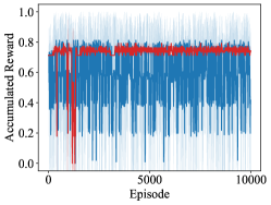
(a) Braking Car

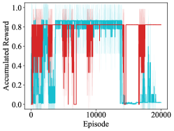
(b) Mountain Car

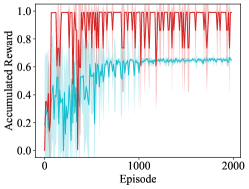
(c) Wumpus World

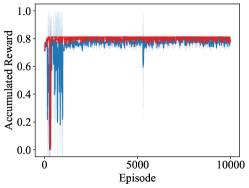
(d) Braking Car

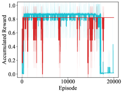
(e) Mountain Car

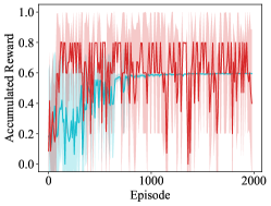
(f) Wumpus World

Figure 6: Normalized cumulative reward per episode while evaluating ten random states (Top), and less likely states (Bottom). The best approach for each case is shown; see figures 9 and 10 for the rest.

(a) Braking Car

(b) MA Navigation

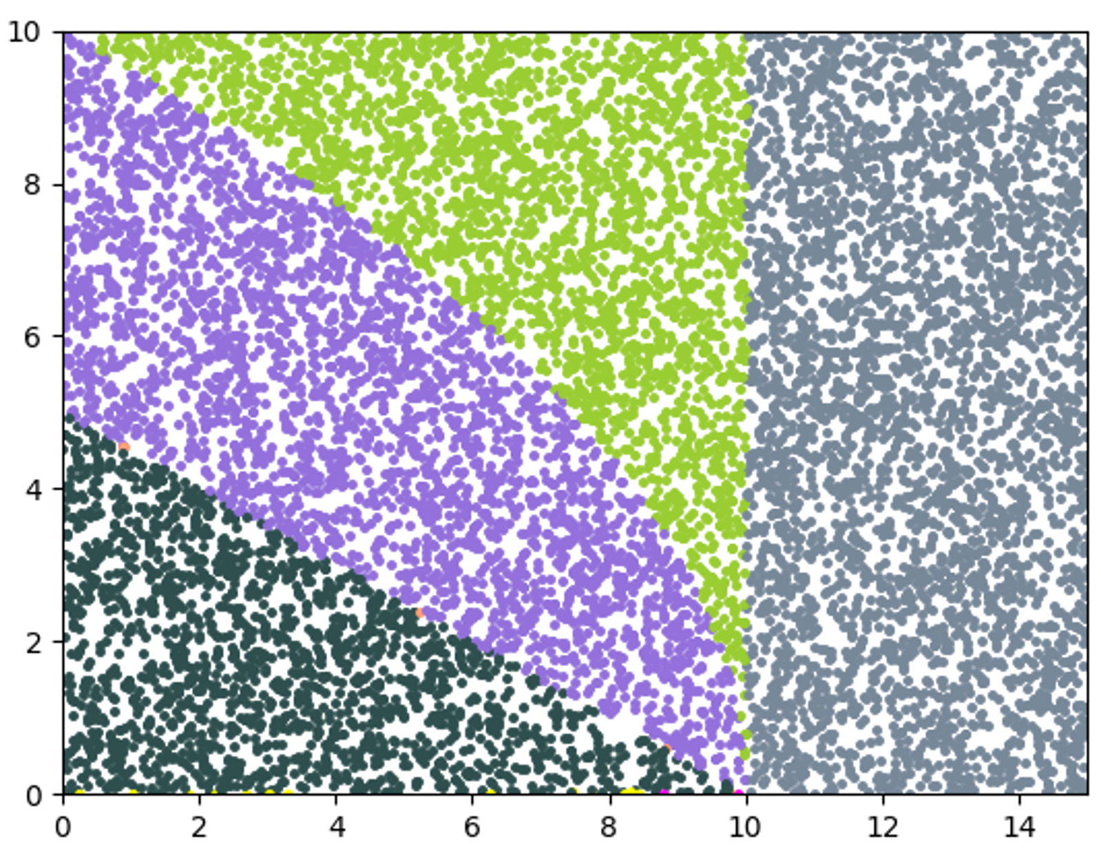
(c) Braking Car

(d) Simple Maze

(e) Random Walk

(f) Simple Maze

Figure 7: Normalized granularity of states and its performance for symbolic execution with search depth $k$ (left and mid). Partitionings with SymPar for the Braking Car and Simple Maze (right).

	SymPar				CAT-RL
	|$\mathcal{S}$ |	Succ	Fail	$\textbf{T}_{\textbf{out}}$	|$\mathcal{S}$ |	Succ	Fail	$\textbf{T}_{\textbf{out}}$
	(#)	(%)	(%)	(%)	(#)	(%)	(%)	(%)
Mountain Car	70	82.2	0.0	17.8	16	78.7	0.0	21.3
Wumpus World 1	73	18.4	0.0	81.6	157	2.7	0.0	97.3
Wumpus World 2	52	37.3	22.9	39.8	22	14.5	30.2	55.3
Braking Car	81	89.1	10.9	0.0	127	34.0	66.0	0.0

Table 2: Partitioning size and learning performance with SymPar and CAT-RL online partitioning.

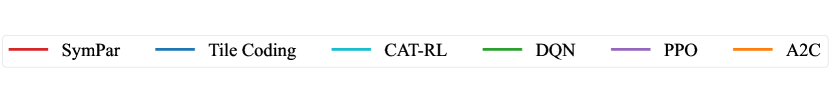
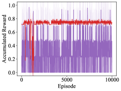
(a) Braking Car

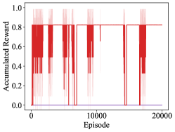
(b) Mountain Car

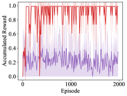
(c) Wumpus World

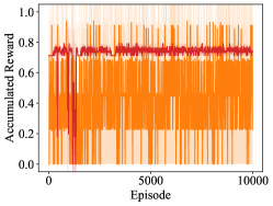
(d) Braking Car

(e) Mountain Car

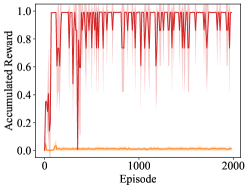
(f) Wumpus World

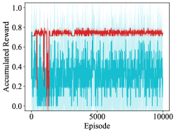
(g) Braking Car

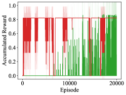
(h) Mountain Car

(i) Wumpus World

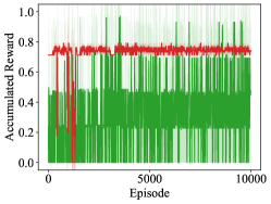
(j) Braking Car

(k) Mountain Car

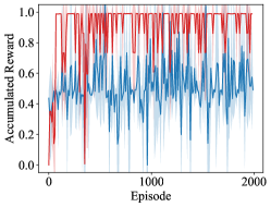
(l) Wumpus World

Figure 9: Normalized cumulative reward per each episode while evaluating ten random states.

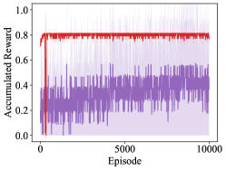
(a) Braking Car

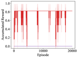
(b) Mountain Car

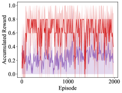
(c) Wumpus World

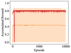
(d) Braking Car

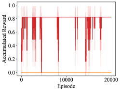
(e) Mountain Car

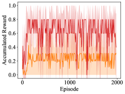
(f) Wumpus World

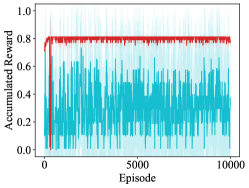
(g) Braking Car

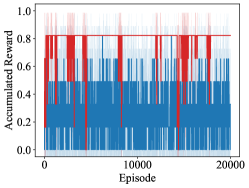
(h) Mountain Car

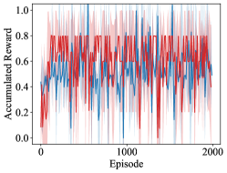
(i) Wumpus World

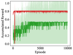
(j) Braking Car

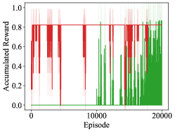
(k) Mountain Car

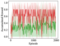
(l) Wumpus World

Figure 10: Normalized cumulative reward per each episode while evaluating ten less likely states.

For randomly selected states, the three top plots in Fig. 6, show that the agents trained by SymPar obtain a better normalized cumulative reward and subsequently converge faster to a better policy than the best competing approaches (other results, cf. Appendix, Fig. 9). The three bottom plots in the figure show the accumulated reward when starting from unlikely states (small partitions) for the best competing approaches (more in Appendix, Fig. 10) Here, we expect to observe a good policy from algorithms that capture the dynamics of environment. Interestingly, the online technique CAT-RL struggles when dealing with large sets of initial states. This can be seen in, e.g., the training for Braking Car, where each episode introduces new positions and velocities.

RQ2.

The four leftmost plots in Fig. 7 show that a higher granularity of partitionings yields a higher accumulated reward achieved with the optimal policy.

The two rightmost plots in Fig. 7 show the shapes of partitions obtained by SymPar for Braking Car and Simple Maze. The first plot represents different partitions with different colors. Notably, the green and purple partitions depict partitioning expressions that contain a non-linear relation between the components of the state space (position and velocity). Besides, close to the x-axis, narrow partitions are discernible, depicted in yellow and pink. To illustrate the partitions obtained for Simple Maze, the expressions are translated into a $10\!\times\!10$ grid. The maze used for Fig. 7(f) differs from the one before, by including additional obstacles in the environment. These two visualizations shed light on the intricacies of state space partitioning and hint at the logical explainability of the partitionings obtained by SymPar.

RQ3.

Table 3 (left) shows that the number of SymPar partitions is independent of the size of the state space. However, this does not imply the universal applicability of the same partitioning across different sizes. The conditions specified within the partitions are size-dependent. Consequently, when analyzing environments with different sizes for a given problem, running SymPar is necessary to ensure the appropriate partitioning, even though the total number of partitions remains the same.

	|$\overline{\mathcal{S}}$|	|$\mathcal{S}$ ​|		|$\overline{\mathcal{S}}$|	|$\mathcal{S}$ ​|		|$\overline{\mathcal{S}}$|	|$\mathcal{S}$ ​|
Simple Maze	$10\!\times\!10$	33	​Wumpus World	$64\!\times\!64$	73	Navig.	$10\!\times\!10$	51
	$10^{2}\!\times\!10^{2}$	33		$10^{2}\!\times\!10^{2}$	73		$10^{2}\!\times\!10^{2}$	51
	$10^{3}\!\times\!10^{3}$	33		$10^{3}\!\times\!10^{3}$	73		$10^{3}\!\times\!10^{3}$	51

	Off	Auto	Dyn	NonL	NarrP	SInd
SymPar	✓	✓	✓	✓	✓	✓
CAT-RL	$\times$	✓	✓	$\times$	$\times$	$\times$
Tiling	✓	$\times$	$\times$	$\times$	$\times$	$\times$

Table 3: Left: Size of state space and partitioning for test problems. Right: Capabilities and properties.

Summary.

Our experiments show distinct advantages of SymPar over the other approaches, cf. Tbl. 3 (right). It is an offline (Off) automated (Auto) approach, which captures the dynamics of the environment (Dyn), and maps the nonlinear relation between components of the state into their representation (NonL). SymPar can detect narrow partitions (NarrP) without excessive sampling and generates a logical partitioning that is independent of the specific size of the state space (SInd). This comprehensive comparison underscores the robust capabilities of SymPar across various dimensions, positioning it as a versatile and powerful approach compared to CAT-RL and Tile Coding.

Limitations.

SymPar can handle only environments that are implemented as programs. It will also perform weakly in environments with very limited branching; e.g., like Cart Pole [5]. The simulation of Cart Pole only branches on final states; its dynamics is a physical formula over the position and velocity of the cart, and the angle and angular velocity of the pole. The path conditions found by symbolic execution are of little help here.

6 Appendix / Supplementary Material

6.1 Technical Details.

The implementation of SymPar uses Symbolic PathFinder [25] as its symbolic executor, Z3 [46] as its main SMT-Solver and the SMT-solver DReal [47] to handle non-linear functions such as trigonometric functions.

6.2 Specification of SymPar

Here, we explain how to create an example in our setting.

First thing you should do is to make a new folder in the directory that JPF has been stetted, otherwise you should make few changes in the JPF settings. So, you need to create a folder in the following directory $./jpf/jpf-symbc/src/examples/partitioning/projectName/$. The directory must be as following

for tree= font=, grow’=0, child anchor=west, parent anchor=south, anchor=west, calign=first, edge path= [draw, edge] (!u.south west) +(7.5pt,0) |- node[fill,inner sep=1.25pt] (.child anchor)edge label; , before typesetting nodes= if n=1 insert before=[,phantom] , fit=band, before computing xy=l=15pt, [projectName [build.xml] [example.jpf] [ClassName4JPF.java] ]

Now, we will explain how each file must look like. Let’s start with the build.xml.

⬇

<project default="compile">

<target name="compile">

<mkdir dir="bin"/>

<javac srcdir="src" destdir="bin" debug="true" debuglevel="lines,vars,source" includeantruntime="false"

classpath="DIRECTORY TO THE JPF ROOT/jpf/jpf-symbc/build/jpf-symbc-classes.jar:DIRECTORY TO THE JPF ROOT/jpf/jpf-core/build/jpf.jar"/>

</target>

</project>

The only change you need to make is that you should update the directory to the path that your JPF has been installed. Next, example.jpf file should be as following

⬇

target=JCar4JPF

classpath=\${jpf-symbc}/build/examples

sourcepath=\${jpf-symbc}/src/examples/partitioning/projectName/

symbolic.dp=CORAL

search.depth_limit = 10

The only necessary modification in this file is $sourcepath$ that must point to the project directory. You also can modify your preferred SMT-solver as $symbolic.dp$ , and depth of search by setting $search.depth_{l}imit$. Note that setting the depth of search in our configuration is also possible.

The next step is creating $ClassName4JPF.java$ and updating it based on your problem and the environment simulation.

⬇

import gov.nasa.jpf.symbc.Debug;

public class ClassName4JPF {

public static void main(String[] args) {;

double x1 = 0.0;

double x2 = 0.0;

double action = 0.0;

x1 = Debug.addSymbolicDouble(x1, "symVar[0]");

x2 = Debug.addSymbolicDouble(x2, "symVar[1]");

ClassName4JPF exmpObj = new ClassName4JPF();

State s1 = exmpObj.step(x1, x2, action);

exmpObj.reward(s1.x1, s1.x2, action);

Debug.printPC("PC");

}

public State step(double x1, double x2, double a){

// step function should be implemented here

}

public double reward(double x1, double x2, double a){

// reward function should be implemented here

}

public double min(double x, double y) {

if (x <= y) return x;

else return y;

}

public double max(double x, double y) {

if (x <= y) return y;

else return x;

}

private class State {

double x1;

double x2;

public State(double x1’, double x2’) {

x1 = x1’;

x2 = x2’;

}

}

}

Figure 8: ClassName4JPF.java

An abstract class of the environment that must be created has been shown in Fig. 8. In this example, we assumed that state has two components ($x1,x2$) and their type is $double$ but you can create your example for other types (integers, boolean, etc) as well.

6.3 Proofs of properties of SymPar

Theorem 1.

The obtained partitioning $\mathcal{P}$ is total for loop-free programs:

$$\forall\overline{s}\in\overline{\mathcal{S}}\cdot\;\exists!\,\mathcal{P}_{0}\in\mathcal{P}\cdot\;\overline{s}\in\mathcal{P}_{0}.$$

Proof.

The theorem follows from the fact that the partitioning generated by SymPar is obtained from first running the simulated environment symbolically and collecting the path conditions. By design, all path conditions produced by a complete terminating symbolic execution run is a partitioning. The final partitioning is obtained by intersecting these partitionings to obtain the unique coarsest partitioning finer than each of them. This partitioning is known from order theory [36] to be unique and it is total and pairwise disjoint. Hence, it can be inferred that each concrete state in the partitioned state space, $\overline{s}\in\overline{\mathcal{S}}$, is represented by at least one partition $\mathcal{P}_{0}\in\mathcal{P}$.∎

Theorem 2.

Let $\mathit{PC}^{a}$ be the set of path conditions produced by SymPar for each of the actions $a\in\mathcal{A}$. The size of the final partitioning $\mathcal{P}$ returned by SymPar is bounded from below by each $|\mathit{PC}^{a}|$ and from above by $\prod_{a\in\mathcal{A}}|\mathit{PC}^{a}|$.

Proof.

The theorem follows from the fact that $\mathcal{P}$ is finer than any of the $\mathit{PC}^{a}$s and the algorithm for computing the coarsest partitioning finer then a set of partitionings can in the worst case intersect each partition in each set $PC^{a}$ with all the partitions in the partitionings of the other actions. ∎

6.4 System Information

We provide the information of the system that has been used for running the experiments.

• OS: macOS-14.4.1-x86_64-i386-64bit Darwin Kernel Version 23.4.0

• Python: 3.11.6

• Stable-Baselines3: 2.2.1

• PyTorch: 2.1.2

• GPU Enabled: False

• Numpy: 1.24.3

• Cloudpickle: 2.2.1

• Gymnasium: 0.29.1

• OpenAI Gym: 0.26.2

6.5 DQN, PPO, and A2C Settings

DQN: "MlpPolicy", train_freq=16, gradient_steps=8, gamma=0.99, exploration_fraction=0.2, exploration_final_eps=0.07, target_update_interval=600, learning_starts=1000, buffer_size=10000, batch_size=128, learning_rate=4e-3, net_arch=[256, 256].

PPO: "MlpPolicy", env, verbose=0, gamma=0.99, batch_size=128, learning_rate=4e-3, net_arch=[256, 256].

A2C: "MlpPolicy", gamma=0.99, learning_rate=4e-3, net_arch=[256, 256].

6.6 Additional Results

To make the comparison with DQN, A2C and PPO fair, we used the same running time as for SymPar, which resulted in lower performance for these approaches. The fluctuation observed in the plots suggest that they may need more iterations and possibly more customized architectures. A2C and PPO, which are proper for problems with continuous action space, behave as expected.

References

- [1] Jens Kober, J Andrew Bagnell, and Jan Peters. Reinforcement learning in robotics: A survey. The Intl. Journal of Robotics Research, 32(11):1238–1274, 2013.
- [2] István Szita. Reinforcement learning in games. In Reinforcement Learning, volume 12 of Adaptation, Learning, and Optimization, pages 539–577. Springer, 2012.
- [3] Mohsen Ghaffari and Mohsen Afsharchi. Learning to shift load under uncertain production in the smart grid. Intl. Transactions on Electrical Energy Systems, 31(2):e12748, 2021.
- [4] Chao Yu, Jiming Liu, Shamim Nemati, and Guosheng Yin. Reinforcement learning in healthcare: A survey. ACM Computing Surveys (CSUR), 55(1):1–36, 2021.
- [5] Richard S. Sutton and Andrew G. Barto. Reinforcement Learning: An Introduction. The MIT Press, 2nd edition, 2018.
- [6] Svitlana Vyetrenko and Shaojie Xu. Risk-sensitive compact decision trees for autonomous execution in presence of simulated market response. arXiv preprint arXiv:1906.02312, 2019.
- [7] Prashan Madumal, Tim Miller, Liz Sonenberg, and Frank Vetere. Explainable reinforcement learning through a causal lens. In Proc. 34th Conf. on Artificial Intelligence (AAAI 2020), pages 2493–2500. AAAI Press, 2020.
- [8] Erika Puiutta and Eric M. S. P. Veith. Explainable reinforcement learning: A survey. In Proc. 4th Intl. Cross-Domain Conf. (CD-MAKE 2020), volume 12279 of Lecture Notes in Computer Science, pages 77–95. Springer, 2020.
- [9] Amber E. Zelvelder, Marcus Westberg, and Kary Främling. Assessing explainability in reinforcement learning. In Proc. Third Intl. Workshop on Explainable and Transparent AI and Multi-Agent Systems (EXTRAAMAS 2021), volume 12688 of Lecture Notes in Computer Science, pages 223–240. Springer, 2021.
- [10] Nathan Fulton and André Platzer. Safe reinforcement learning via formal methods: Toward safe control through proof and learning. In Proc. 32nd Conf. on Artificial Intelligence (AAAI-18), pages 6485–6492. AAAI Press, 2018.
- [11] Cees F. Verdier, Robert Babuška, Barys Shyrokau, and Manuel Mazo. Near optimal control with reachability and safety guarantees. IFAC-PapersOnLine, 52(11):230–235, 2019.
- [12] Andreas Dyrøy Jansson. Discretization and representation of a complex environment for on-policy reinforcement learning for obstacle avoidance for simulated autonomous mobile agents. In Proc. 7th Intl. Congress on Information and Communication Technology, volume 464 of Lecture Notes in Networks and Systems, pages 461–476. Springer, 2023.
- [13] Peng Jin, Jiaxu Tian, Dapeng Zhi, Xuejun Wen, and Min Zhang. Trainify: A CEGAR-driven training and verification framework for safe deep reinforcement learning. In Proc. 34th Intl. Conf. on Computer Aided Verification (CAV 2022), volume 13371 of Lecture Notes in Computer Science, pages 193–218. Springer, 2022.
- [14] Hoang-Dung Tran, Feiyang Cai, Manzanas Lopez Diego, Patrick Musau, Taylor T Johnson, and Xenofon Koutsoukos. Safety verification of cyber-physical systems with reinforcement learning control. ACM Transactions on Embedded Computing Systems (TECS), 18(5s):1–22, 2019.
- [15] Julius Adelt, Paula Herber, Mathis Niehage, and Anne Remke. Towards safe and resilient hybrid systems in the presence of learning and uncertainty. In Proc. 11th Intl. Symposium on Leveraging Applications of Formal Methods, Verification and Validation. Verification Principles (ISoLA 2022), volume 13701 of Lecture Notes in Computer Science, pages 299–319. Springer, 2022.
- [16] Manfred Jaeger, Peter Gjøl Jensen, Kim Guldstrand Larsen, Axel Legay, Sean Sedwards, and Jakob Haahr Taankvist. Teaching Stratego to play ball: Optimal synthesis for continuous space MDPs. In Proc. 17th Intl. Symposium on Automated Technology for Verification and Analysis (ATVA 2019), volume 11781 of Lecture Notes in Computer Science, pages 81–97. Springer, 2019.
- [17] Ivan SK Lee and Henry YK Lau. Adaptive state space partitioning for reinforcement learning. Engineering applications of artificial intelligence, 17(6):577–588, 2004.
- [18] Haoran Wei, Kevin Corder, and Keith Decker. Q-learning acceleration via state-space partitioning. In Proc. 17th Intl. Conf. on Machine Learning and Applications (ICMLA 2018), pages 293–298. IEEE, 2018.
- [19] Riad Akrour, Filipe Veiga, Jan Peters, and Gerhard Neumann. Regularizing reinforcement learning with state abstraction. In Proc. Intl. Conf. on Intelligent Robots and Systems (IROS), pages 534–539. IEEE, 2018.
- [20] Christos N Mavridis and John S Baras. Vector quantization for adaptive state aggregation in reinforcement learning. In 2021 American Control Conf. (ACC), pages 2187–2192. IEEE, 2021.
- [21] Sam Nicol and Iadine Chadès. Which states matter? an application of an intelligent discretization method to solve a continuous POMDP in conservation biology. PloS one, 7(2):e28993, 2012.
- [22] Mehdi Dadvar, Rashmeet Kaur Nayyar, and Siddharth Srivastava. Conditional abstraction trees for sample-efficient reinforcement learning. In Proc. 39th Conf. on Uncertainty in Artificial Intelligence, volume 216 of Proc. Machine Learning Research, pages 485–495. PMLR, 2023.
- [23] James C King. Symbolic execution and program testing. Communications of the ACM, 19(7):385–394, 1976.
- [24] Lori A. Clarke. A program testing system. In Proc. 1976 Annual Conf., pages 488–491. ACM, 1976.
- [25] Corina S. Pasareanu, Willem Visser, David H. Bushnell, Jaco Geldenhuys, Peter C. Mehlitz, and Neha Rungta. Symbolic PathFinder: integrating symbolic execution with model checking for Java bytecode analysis. Autom. Softw. Eng., 20(3):391–425, 2013.
- [26] Donald Michie and Roger A Chambers. Boxes: An experiment in adaptive control. Machine intelligence, 2(2):137–152, 1968.
- [27] Andrew W Moore. Variable resolution dynamic programming: Efficiently learning action maps in multivariate real-valued state-spaces. In Machine Learning Proceedings 1991, pages 333–337. Elsevier, 1991.
- [28] James S Albus. Brains, behavior, and robotics. BYTE Books, 1981.
- [29] Pier Luca Lanzi, Daniele Loiacono, Stewart W. Wilson, and David E. Goldberg. Classifier prediction based on tile coding. In Proc. Genetic and Evolutionary Computation Conf. (GECCO 2006), pages 1497–1504. ACM, 2006.
- [30] William T. B. Uther and Manuela M. Veloso. Tree based discretization for continuous state space reinforcement learning. In Proc. 15th National Conf. on Artificial Intelligence and Tenth Innovative Applications of Artificial Intelligence Conf. (AAAI 98, IAAI 98), pages 769–774. AAAI Press / The MIT Press, 1998.
- [31] Shimon Whiteson. Adaptive Representations for Reinforcement Learning, volume 291 of Studies in Computational Intelligence. Springer, 2010.
- [32] Jendrik Seipp and Malte Helmert. Counterexample-guided cartesian abstraction refinement for classical planning. Journal of Artificial Intelligence Research, 62:535–577, 2018.
- [33] Frank S. de Boer and Marcello M. Bonsangue. Symbolic execution formally explained. Formal Aspects Comput., 33(4-5):617–636, 2021.
- [34] Erik Voogd, Einar Broch Johnsen, Alexandra Silva, Zachary J Susag, and Andrzej Wąsowski. Symbolic semantics for probabilistic programs. In Proc. 20th Intl. Conf. on Quantitative Evaluation of Systems (QEST 2023), volume 14287 of Lecture Notes in Computer Science, pages 329–345. Springer, 2023.
- [35] Cristian Cadar, Daniel Dunbar, and Dawson R. Engler. KLEE: unassisted and automatic generation of high-coverage tests for complex systems programs. In Proc. 8th Symposium on Operating Systems Design and Implementation (OSDI 2008), pages 209–224. USENIX Association, 2008.
- [36] Brian A. Davey and Hilary A. Priestley. Introduction to lattices and order. Cambridge University Press, Cambridge, 1990.
- [37] Dexter Kozen. Semantics of probabilistic programs. In Proc. 20th Annual Symposium on Foundations of Computer Science (SFCS 1979), pages 101–114. IEEE Computer Society, 1979.
- [38] Volodymyr Mnih, Koray Kavukcuoglu, David Silver, Alex Graves, Ioannis Antonoglou, Daan Wierstra, and Martin Riedmiller. Playing Atari with deep reinforcement learning. arXiv preprint arXiv:1312.5602, 2013.
- [39] Volodymyr Mnih, Adrià Puigdomènech Badia, Mehdi Mirza, Alex Graves, Timothy P. Lillicrap, Tim Harley, David Silver, and Koray Kavukcuoglu. Asynchronous methods for deep reinforcement learning. In Proc. 33nd Intl. Conf. on Machine Learning (ICML 2016), volume 48 of JMLR Workshop and Conf. Proceedings, pages 1928–1937. JMLR.org, 2016.
- [40] John Schulman, Filip Wolski, Prafulla Dhariwal, Alec Radford, and Oleg Klimov. Proximal policy optimization algorithms. arXiv preprint arXiv:1707.06347, 2017.
- [41] Antonin Raffin, Ashley Hill, Maximilian Ernestus, Adam Gleave, Anssi Kanervisto, and Noah Dormann. Stable baselines3, 2019. https://stable-baselines3.readthedocs.io/.
- [42] Mahsa Varshosaz, Mohsen Ghaffari, Einar Broch Johnsen, and Andrzej Wąsowski. Formal specification and testing for reinforcement learning. Proc. ACM Program. Lang., 7(ICFP), aug 2023.
- [43] Guni Sharon, Roni Stern, Ariel Felner, and Nathan R Sturtevant. Conflict-based search for optimal multi-agent pathfinding. Artificial Intelligence, 219:40–66, 2015.
- [44] Andrew W. Moore. Efficient memory-based learning for robot control. PhD thesis, University of Cambridge, UK, 1990.
- [45] Stuart J Russell and Peter Norvig. Artificial intelligence a modern approach. London, 2010.
- [46] Leonardo Mendonça de Moura and Nikolaj S. Bjørner. Z3: an efficient SMT solver. In Proc. 14th Intl. Conf. on Tools and Algorithms for the Construction and Analysis of Systems (TACAS 2008), volume 4963 of Lecture Notes in Computer Science, pages 337–340. Springer, 2008.
- [47] Sicun Gao, Soonho Kong, and Edmund M. Clarke. dReal: An SMT solver for nonlinear theories over the reals. In Proc. 24th Intl. Conf. on Automated Deduction (CADE-24), volume 7898 of Lecture Notes in Computer Science, pages 208–214. Springer, 2013.