Hierarchy of percolation patterns in a kinetic replication model
Abstract
The model of a one-dimensional kinetic contact process with parallel update is studied by the Monte Carlo simulations and finite-size scaling. The goal was to reveal the structure of the hidden percolative patterns (order parameters) in the active phase and the nature of transitions those patterns emerge through. Our results corroborate the earlier conjecture that in general the active (percolating) phases possess the hierarchical structure (tower of percolation patterns), where more complicated patterns emerge on the top of coexistent patterns of lesser complexity. Plethora of different patterns emerge via cascades of continuous transitions. We detect five phases with distinct patterns of percolation within the active phase of the model. All transitions on the phase diagram belong to the directed percolation universality class, as confirmed by the scaling analysis. To accommodate the case of multiple percolating phases the extension of the Janssen-Grassberger conjecture is proposed.
I Introduction
Percolation is an example of phase transition involving nonlocal order which probes connectivity of a system [1]. The evolution of many kinetic models (kinetic contact process with parallel update, probabilistic cellular automata, PCA) in (space-time) dimensions results in 2D directed percolative landscapes. The applications of such models range from statistical physics, critical phenomena, condensed matter to biology, ecology, quantitative finance or network theory [2, 3, 4, 5, 6, 7, 8].
It has been shown [9, 10] that the active (percolating) phases of several kinetic processes and some other 2D models of percolation possess numerous hidden geometric orders characterized by distinct order parameters (percolative patterns/backbones), emerging at specific critical points of continuous phase transitions. The order parameters are the capacities of corresponding backbones spanning through whole system in the time direction (or, equivalently, the density of the connected active sites in the stable state of directed processes). These transitions belong to the directed percolation (DP) universality class, and they are confirmed unambiguously [10] even for the well-known DP and contact process models which have been studied for about five decades or so [2, 3].
The multitude of conceivable percolation patterns (phases) implies the existence of (infinite) cascades of geometric transitions in the parametric space. Moreover, the hierarchical structure (tower of percolation patterns) is a generic feature of percolating phase, and it should be looked for in other models of statistical mechanics and kinetics. This is a very important conclusion for the whole theory of percolation. More broadly, such hierarchy should exist in a generic distributed system/network and can be used to quantify its connectedness. This hypothesis has vast implications for different fields, and in particular for networks.
Network science is a very active interdisciplinary field with virtually ubiquitous applicability. It ranges from telecommunications, electric power supply, Internet, warehouse logistics, transportation, engineering to physics, biology, neurology, and sociology [11, 5, 12, 13, *Sporns:2012, 6, 15, 16]. The proper functioning and resilience of networks are of great importance, and many studies have been devoted to their robustness against various kinds of damage [5, 17, *Stanley:2012, *Stanley:2013].
One of the motivations to study the hidden structure of the active phases of processes or 2D percolation landscapes, is to reveal a similar hierarchy in generic networks. The latter by the very construction are assumed to be connected, i.e., they are in the percolating phase (if the thermodynamic limit is understood).
The conjecture [10] that there is potentially an infinite number of percolation backbones (patterns) in a smoothly evolving percolating phase is not rigorously proven. But even if so, construction of an infinite tower of percolation patterns is not very practical or useful for comparative analysis of percolation landscapes or their resilience; two problems very relevant for applications. The important task is to construct a judicious case-motivated set of percolative patterns to classify a given landscape.
The percolative backbone (pattern) is defined [10] as percolation on the backbone cluster spanning through whole system. This cluster consists of renormalized (coarse-grained) nodes made out of a subset of nodes of the original lattice (graph).111These ideas are somehow similar to the earlier proposals of high-density [20, 21, 22] or -clique percolation
[23, *Derenyi:2007] on different lattices, graphs or networks. Similar notions of “motifs” were used in the context of brain connectivity [12, *Sporns:2012]
We should point out that the multiple transitions found in networks or other models of percolation differ from those reported here and in [9, 10], since the former are either related to the singularities of a single order parameter or due to coupling of different networks.
The percolation in the backbone occurs with respect to the bonds connecting active nodes of the backbone cluster.222In case of 2D lattice considered in the present work, the backbone cluster can be simply called the renormalized lattice.
There are two points to be clarified in the above definition:
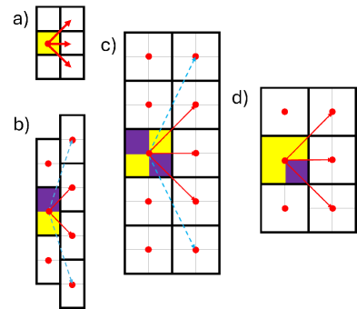
1). The attribution of activity to the renormalized node (filled/empty) allows different choices. For instance, for the case of plaquettes to be identified as new renormalized nodes, one can select a particular half-filled configuration (quadrupole) as an active renormalized node and discard all other fillings as a renormalized empty state; or select a configuration where plaquette is either fully filled or one out of four original sites is empty, see Fig. 1.
2). The bonds between renormalized sites do not need to coincide with their counterparts in the original lattice. This is plainly obvious in the context of networks: say, on the map of a town one can consider a backbone cluster of acquainted couples. Or, for the model considered in this work: its spreading rules allow to admit percolating bonds (due to correlations) between the nearest and next-nearest renormalized nodes.
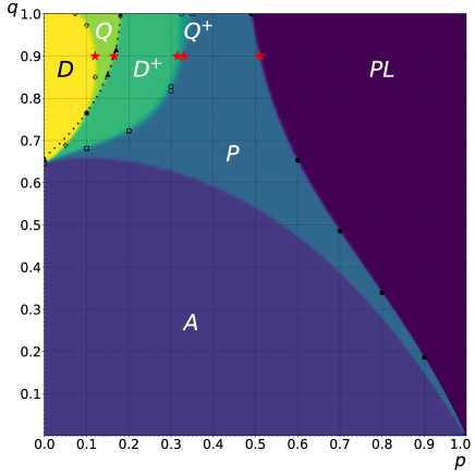
To build up working algorithms for unfolding the hidden hierarchy of percolative patterns, we will study the replication model (a version of PCA) proposed in [9]. The attractive feature of this model is that its active phase demonstrates evolution in the parametric space from quite distinguished antiferromagnetic-like pattern to a fully occupied lattice. This was suggestive [9] for the search of a new phase (denoted as in Fig. 2) with the dipole percolating pattern within the active phase. In this paper we report six distinct percolating phases on the phase diagram of the model. The results demonstrate clearly the key role of both elements in the emergence of a percolating backbone: 1) local order of primary sites within a renormalized node; 2) the range of percolation admitted between locally ordered (that is active) nodes of the backbone.
II Model and Methods
In this paper we study a one-dimensional kinetic contact replication process (a version of probabilistic cellular automaton, PCA). The state of the system at discrete time step is specified by the occupation numbers (filled/empty), , with periodic boundary conditions (PBC) in the spatial direction. At the initial random configuration of -s is cast. The Monte Carlo simulations with parallel update (i.e., the configurations at all sites are updated simultaneously in one time step) are used to numerically mimic stochastic evolution of the model. The latter is governed by the transfer probabilities defined as the probability to have a filled site at the time given the configuration of neighboring sites , , and at the time . We denote it as . The model’s transfer probabilities are:
| (1) |
The above probabilistic rules of the model are presented in Table 1 and visualized in Fig. 1a. The kinetic process (1) can be considered as directed percolation on the (1+1) (space-time) lattice shown in Fig. 1; its absorbing (active) phase is non-percolative (percolative) phase on the 2D lattice, respectively. This model was introduced and studied in [9]. It can be considered as a modification of the well-known model of the directed bond percolation (BDP) [2].
|
|
|
|
|
|
|
|
|
|
|||||||||||||||||||||||||||
|---|---|---|---|---|---|---|---|---|---|---|---|---|---|---|---|---|---|---|---|---|---|---|---|---|---|---|---|---|---|---|---|---|---|---|---|
|
The absorbing-active phase transition is probed by the order parameter
| (2) |
where denotes averaging over random trials, such that in the absorbing phase, while in the active phase . In spite of the seemingly local form of , it detects nonlocal ordering in the active phase giving simultaneously the probability of existence of a path (string) [10] connecting active sites in the time interval . This is a consequence of the fact that every filled site must have at least one ancestor at the preceding time step, as follows from the transfer probabilities of the model (1).
For transitions with a local order parameter, coarse graining (e.g., the Kadanoff-Wilson scheme) cannot yield new critical points, i.e., the coarse-grained and the original order parameters appear simultaneously. It has been numerically confirmed for several models [10] that the same is not true for nonlocal percolation order. Coarse graining implemented via construction of a new percolative backbone made out of some connected subsets (mini-clusters) of the original sites engenders cascades of transitions when distinct percolative patterns (order parameters) emerge within the active phase.
We will study the critical properties of the model (1) using the finite-size scaling analysis of the raw MC data. For the DP class transition one needs three independent exponents [2]. In the active phase the order parameter near the absorbing-active transition scales as:
| (3) |
and similarly with , depending on the chosen direction in the parametric plane . The dynamical transition is characterized by the spatial () and the temporal () correlation lengths, diverging at the critical point as:
| (4) |
Two correlation lengths are related through the dynamical exponent
| (5) |
For a finite-size system the order parameter scales as [2]:
| (6) |
where is the distance from the critical point, and the exponent
| (7) |
determines the critical decay of at in the limit .
From analysis of (6) with various data sets, we infer the critical points and the indices , , and , as explained in the next section. Once and are found, the value of is calculated from (7).
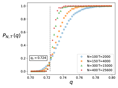
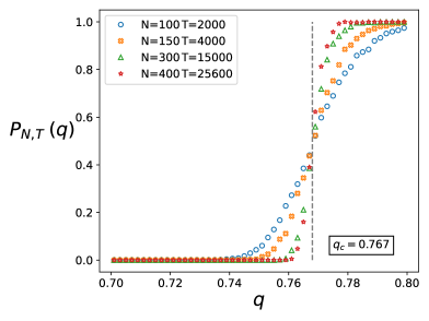
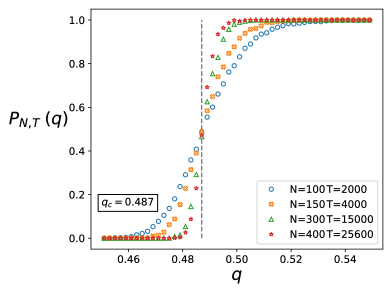
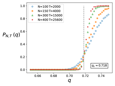
As an independent cross-check for the location of the critical points found from (6), we also calculate the probability that a connected cluster spanning from to occurs in the system of size . is simply given by the fraction of connected sites, and it is an analogue of the Binder cumulant for percolation [25]. For a given value of , plots of for different sizes , all intersect at the critical point .
III Results
III.1 Active and dipole phases
The absorbing-active transition and the transition within the active (percolating) phase into the phase with dipole percolation pattern were reported in the earlier work [9]. The current results confirm those phase boundaries on the phase diagram in Fig. 2 and the DP universality class of both transitions. The attributes of the active phase are standard [2], below we recapitulate the definition of the dipole phase to make the presentation more self-contained and to better explain some sticky points of [9].
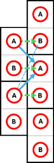
To understand the simulation results given below, let us first get some intuitive understanding of the model. In the limit it is equivalent to the directed bond percolation (BDP) with the percolating threshold . The BDP is taking place on two sublattices ( and ) shown in Fig. 3. The two sublattices are correlated due to the term . Moreover, since , -replication promotes the active phase with alternated filling in the spatial and temporal directions. At the other end of the active phase when (), the stable state is a fully occupied lattice in both directions. The above arguments suggest that at least one transition could occur in the range to separate two active phases with distinct percolation patterns.
The mean-field solution of the master equation [9] predicts a continuous transition in the region of small inside the active phase. The transition separates a phase with uniform filling in the stationary state at from the “antiferromagnetic” (AFM) phase with different subblattice occupations , in both directions at . In the limit , one of the sublattices stays empty (or ). The mean-field approximation leads to the spontaneous breaking of sublattice symmetry .
The MC simulations disprove the mean-field prediction of the local AFM order with the occupancy disproportionation, but the mean field is suggestive to reveal a true and more subtle transition between the percolative patterns in the active phase. A simply percolating phase (we will call it just “percolated” () in the following) is detected by the non-vanishing standard order parameter (2). To reveal the other percolating phase we need to coarse grain the sites of the original lattice (or to single out a new percolative backbone, as defined in [10]). To deal with the dipole (AFM) percolating phase we proceed as follows: for a given 2D () MC data set we analyse the connectivity of the dipoles residing on the nodes of the dipole lattice shown in Fig. 1b. The occupation numbers on the sites of the coarse-grained (dipole) lattice for the four possible dipole configurations are defined as follows:
| (12) | |||||
| (17) |
The percolation (connectivity) on the dipole latticecan be allowed between the nearest neighboring (nn) and the next-nearest neighboring (nnn) active sites. The site on the coarse grained lattice is active if a dipole resides on it, . A more loosed connectivity (percolation) between nnn dipoles is introduced to account for the correlations occurring due to -transfer probabilities, as shown in Fig. 3. In this work we study two dipole phases: phase is the one where the percolation only between nn dipoles is accounted for; and in phase the percolation patterns include bonds between the nn and nnn active sites. The latter phase was first detected in [9].
To determine the lines of phase transitions and critical indices we run MC simulations according to the rules (1) for different sets of sizes and time steps , averaging each set over 1000 trials. The line of the absorbing-percolating phase transition, see Fig. 2, reproduces exactly the result of [9] along with the critical indices of the DP universality class.
| z | ||||||
|---|---|---|---|---|---|---|
| 0.0000 | 0.6444 | 0.1595 | 1.72 | 1.58 | 0.27(4) | 1.08(8) |
| 0.0500 | 0.6896 | 0.1595 | 1.72 | 1.56 | 0.27(4) | 1.10(2) |
| 0.1000 | 0.7662 | 0.1595 | 1.72 | 1.56 | 0.27(4) | 1.10(2) |
| 0.2002 | 0.8500 | 0.1595 | 1.72 | 1.56 | 0.27(4) | 1.10(2) |
| 0.1000 | 0.9735 | 0.1595 | 1.72 | 1.56 | 0.27(4) | 1.10(2) |
| 0.0736 | 1.0000 | 0.1590 | 1.72 | 1.57 | 0.27(3) | 1.09(5) |
To detect phase inside the active phase we calculate the dipole occupation (17) on the sites of the dipole lattice for each set of 2D MC data () obtained via the process (1) on the original lattice. The appearance of the dipole percolation is signalled by non-vanishing concentration of the active connected dipoles , where is defined analogously to (2). The selection of the active connected dipoles is made iteratively at each time step: The dipole occupation (17) is calculated from the MC results at and . Among the active dipoles only those who have active ancestors, i.e., connected by the nn and/or nnn bonds to , are retained. The disconnected active dipoles are discarded, . The procedure repeats until we reach . The analysis of the phase yields the results in a complete agreement with those reported in earlier work [9], some data and results are given in Appendix.
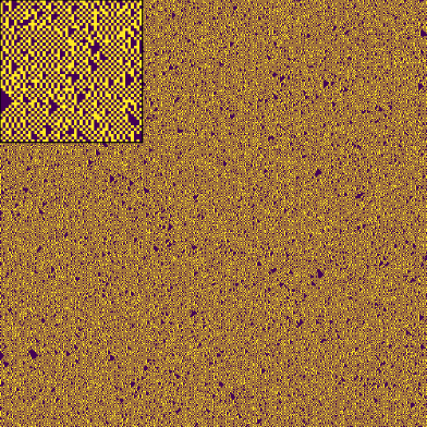
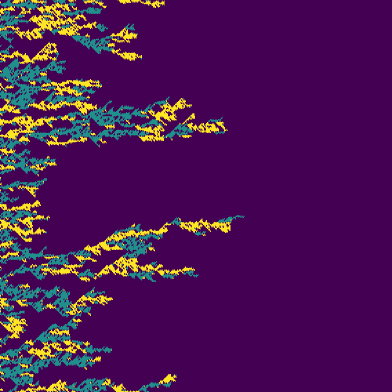
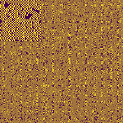
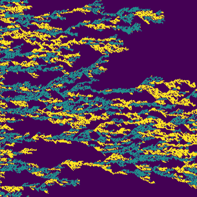
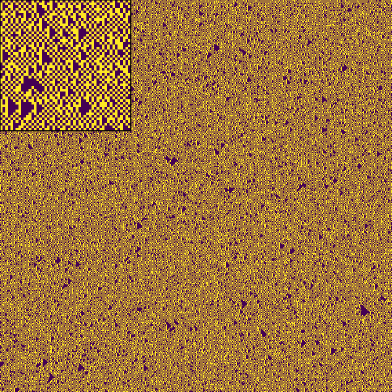
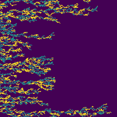
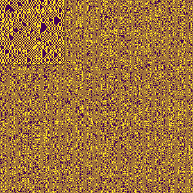
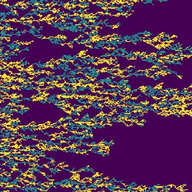
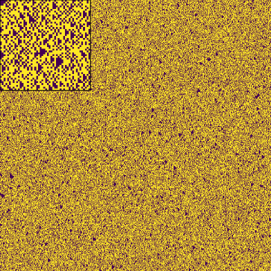
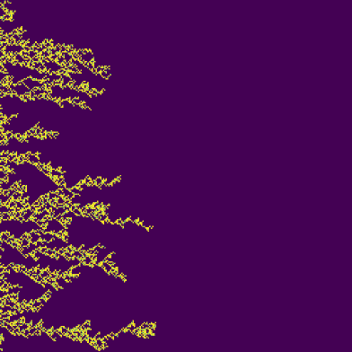
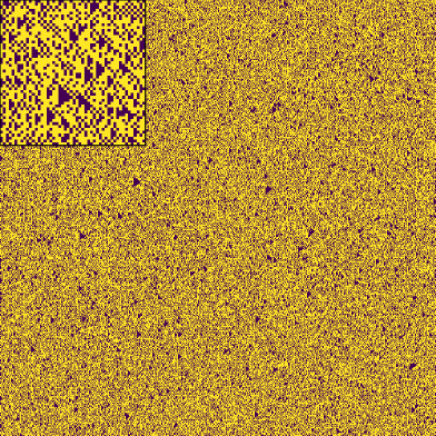
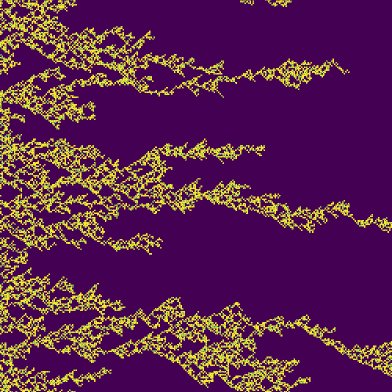
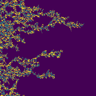
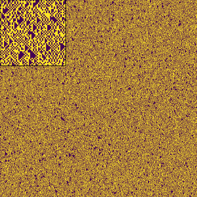
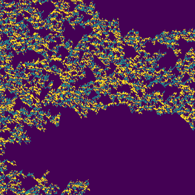
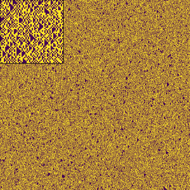
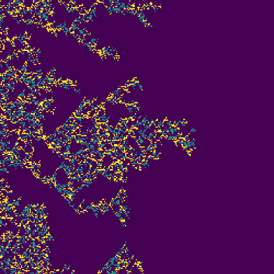
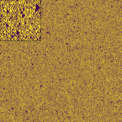
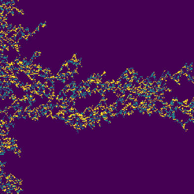
To analyse phase we follow the same steps as above, with the only difference that the active connected dipoles at the time step are selected from those who have active ancestors at , connected by the nn bonds only. In Fig. 4 we show the raw MC results for the original occupancies on two sides from the critical line of the phase. The percolation patterns of the phase (a,c) are visually indistinguishable in both cases, while selection of the dipole percolation pattern with the nn connectivity (nn bonds) demonstrates clearly that the raw patterns are separated by a percolation transition into phase.
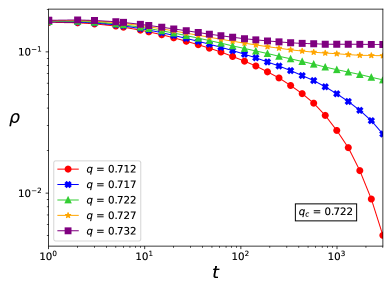
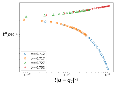
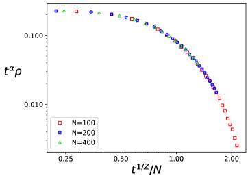
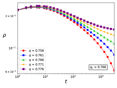
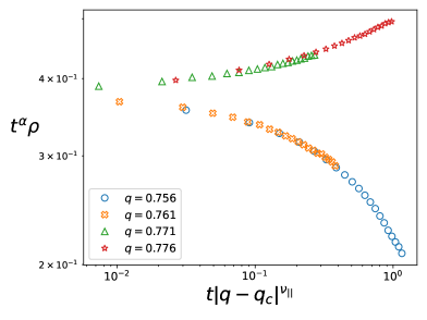
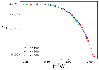
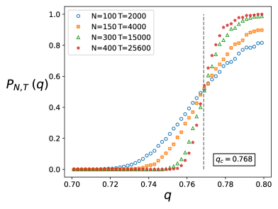
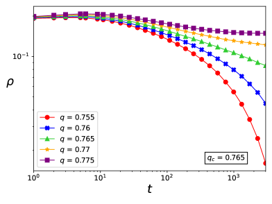
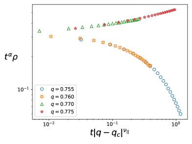
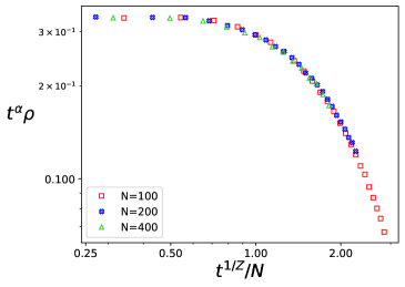
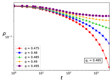
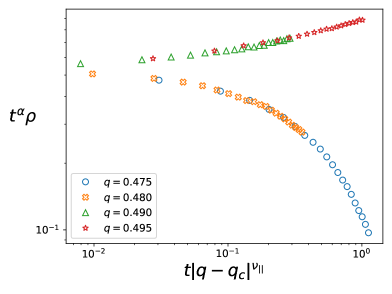
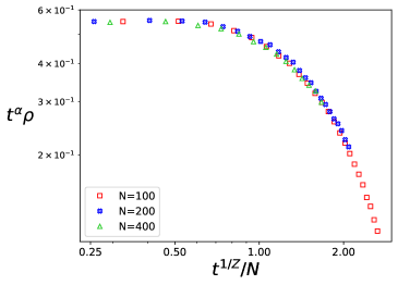
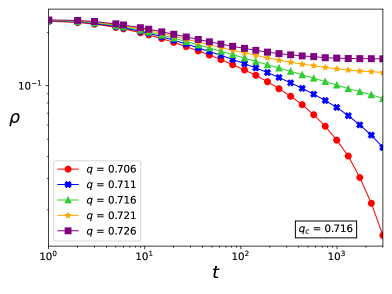
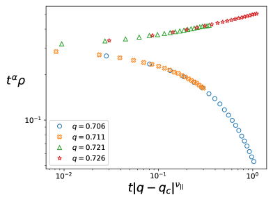
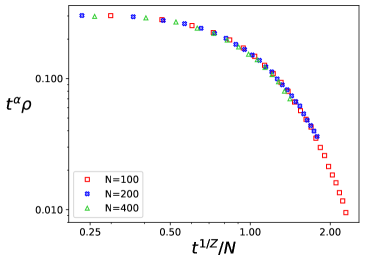
In Fig. 5 (a) is plotted against on a double logarithmic scale.333From now on we keep tildes for the definitions of the coarse-grained occupation numbers, but drop them in graphs, etc, to unclutter notations. From collapse of the scaling functions for the system of different sizes shown in Fig. 5 (b,c), the indices and are obtained. The location of the critical point is also confirmed by the plots of the fraction of connected dipoles for different sizes , shown in Fig. 5 (d). They all intersect at . The boundary of the phase is shown in Fig. 2; numerical results for several critical points and critical indices for the transition into this phase are collected in Table 2. The numbers confirm that this transition belongs to the DP universality class.
III.2 Quadrupole phases
The distinct percolation landscapes of the model in two limiting cases and , discussed in the previous section, are suggestive to propose existence of other percolating phases with new patterns to be called quadrupole. We construct a new percolative backbone on the coarse grained lattice made out of plaquettes (bold lines in Fig. 1c) of the original lattice sites. The nodes of the coarse-grained lattice are placed at the centers of the plaquettes, see Fig. 1c.
The quadrupole occupation numbers on the nodes of the plaquette lattice are defined as:
| (22) | |||||
| (23) |
The site is called active if . Then the procedure and analysis follow the same steps described in detail in the previous subsection. Again, we select two quadrupole percolative patterns: where percolation is allowed between nn and nnn active sites and where percolation is allowed between nn sites only.
| z | ||||||
|---|---|---|---|---|---|---|
| 0.0000 | 0.6564 | 0.1590 | 1.72 | 1.57 | 0.27(3) | 1.09(5) |
| 0.1000 | 0.7656 | 0.1595 | 1.72 | 1.56 | 0.27(4) | 1.10(2) |
| 0.1500 | 0.8557 | 0.1590 | 1.72 | 1.58 | 0.27(3) | 1.08(8) |
| 0.1700 | 0.9161 | 0.1590 | 1.72 | 1.55 | 0.27(3) | 1.10(9) |
| 0.1800 | 1.0000 | 0.1590 | 1.72 | 1.58 | 0.27(3) | 1.08(8) |
The examples of the raw MC data on two sides from the transition are shown in Fig. 6, along the extracted patterns. The latter clearly demonstrate occurrence of transition with the quadrupole percolative pattern. Some examples of the finite-size scaling analysis for the -phase transition are given in Fig. 7. The numerical results for several critical points and critical indices are presented in Table 3.
Similar numerical results for phase are collected in the Appendix. The numbers confirm that both transitions belongs to the DP universality class. The boundaries of the and phases are shown in Fig. 2.
III.3 Plaquette phase
As explained above, in the limit the stable state of the model is a fully occupied lattice in both (space-time) directions. From the above results we expect an intermediate transition between patterns and a fully occupied state. For this end we consider again the coarse grained plaquette lattice shown in Fig. 1d. We will check for the percolation between fully filled plaquettes or those with only one empty corner, see Fig. 1d. We define the plaquette occupation number on the sites of the plaquette lattice as:
| (24) |
where the sum runs over 4 sites of the plaquette, and is the Heaviside step function defined such that and . We will be looking for the phase with percolation between active plaquettes connected by nn bonds ( phase).
| z | ||||||
|---|---|---|---|---|---|---|
| 0.4900 | 1.0000 | 0.1590 | 1.72 | 1.58 | 0.27(3) | 1.08(8) |
| 0.6000 | 0.6256 | 0.1590 | 1.72 | 1.54 | 0.27(3) | 1.11(6) |
| 0.7000 | 0.4854 | 0.1590 | 1.72 | 1.55 | 0.27(3) | 1.10(9) |
| 0.8000 | 0.3395 | 0.1590 | 1.72 | 1.58 | 0.27(3) | 1.08(8) |
| 0.9000 | 0.1865 | 0.1593 | 1.72 | 1.56 | 0.27(4) | 1.10(2) |
Following the procedure used for other phases, we detect phase where it was expected, its location is shown in Fig. 2. Examples of the patterns and scaling analysis near transition are given in Figs. 8 and 9.
The results given in Table 4 confirm the DP universality class of the transition into phase.
IV Conclusion and Discussion
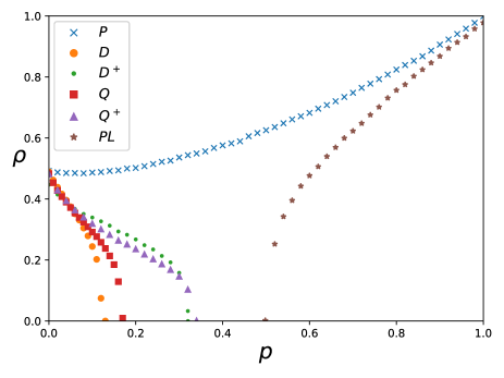
The phase diagram of a one-dimensional kinetic contact process with parallel update is established using the Monte Carlo simulations and finite-size scaling, see Fig. 2. The structure of the hidden percolative patterns (order parameters) emerging through transitions in the active phase and the nature of those transitions are revealed. Our results corroborate the conjecture that in general the active (percolating) phases possess the hierarchical structure (tower of percolation patterns), where more complicated patterns emerge on the top of coexistent patterns of lesser complexity, see Fig. 10. Plethora of different patterns emerge via cascades of continuous phase transitions. We detect five phases with distinct patterns of percolation within the active phase of the model. From the results visualized in Figs. 2 and 10 we infer the following hierarchy in the active phase: at and the model is just percolating, it sits in the “trivial” -phase (see the “flat” non-vanishing -order parameter in the whole region shown in Fig. 10). Moving from there along towards , the tower of coexistent percolative patterns builds in:
as we cross the corresponding critical lines. The percolarive landscape is less rich in the opposite direction:
| (26) |
The hierarchy (IV) and (26) appears to be a judicious set of phases to account for distinct local order seen in the percolating patterns on the parametric plane of the model.
All transitions on the phase diagram belong to the DP universality class, as confirmed by the finite-size scaling analysis. This seems to be at odds with the Janssen-Grassberger (JG) conjecture [26, 27]. The universality classes of various nonequilibrium lattice models are well-classified [28]. In particular, according to the JG conjecture, a model belongs to the DP universality class if it satisfies the following conditions: (i) transition is continuous between a fluctuating active phase and a unique absorbing state; (ii) the order parameter is positive and one-component; (iii) interactions are short-ranged; (iv) no quenched disorder or additional symmetries are present [3]. Apparently the requirement (i) needs to be clarified to accommodate the case of multiple percolating phases. For each active (percolating) phase analyzed, the requirements (ii)-(iv) are satisfied, although the active phase is not unique. The absorbing (empty) state (vacuum ) is unique for each active phase, but those empty states (vacua) are defined with respect to a particular pattern (see Figs. 4,11,6,13 and comments to those figures), so they are distinct states:
| (27) |
The present results suggest an extension of the JG conjecture. It holds if the first condition above is modified as follows:
() transition is continuous between a fluctuating active (percolating) phase and its own unique absorbing (empty) state ; the couple
active-empty state is not unique in general:
, .
Thus far the results on the tower of percolating patterns are deduced from the numerical analysis of simulations. To get a better insight on the origin of the cascades, a promising direction is to relate these transitions to zeros of the non-equilibrium stationary partition functions. Yang and Lee [29, *LeeYang:1952] pioneered this rigorous statistical-mechanical approach to study phase transitions. The theory is applicable whatever are the nature of order parameter or symmetry breaking. It can be extended for the open systems and models out of equilibrium, see, e.g., [31, 32, 33, 34, 35, 36], and more references there. In several equilibrium models [37, *Chitov:2021, *Chitov:2022DL] one can relate the Lee-Yang zeros to the cascades of transitions and also to the spectra of the transfer matrices. So, the goal for the future work is to relate zeros of generalized partition functions of the stationary states to the spectra of transfer matrices deduced from the master equation of the kinetic replication model (1).
On the purely computational side, it is very appealing to work out some machinery for the percolation pattern recognition in the raw MC data. The neural networks/machine learning (for a review, see e.g., [40] and more references there) seems to be a very effective tool for the problems of percolation [41, 42, *Shen:2022] and even for the implementation of the Lee-Yang approach [44]. Some progress has been made recently in applying neural networks to detect the percolation patterns of model (1), to be reported elsewhere.
The networks is the field where the above ideas and approaches can be most naturally applied and advanced. The connectivity of a network (empirical or model-generated), that is its functionality, can be quantitatively classified by its tower of the patterns of connectivity. One of the very important practical problem in generic networks (e.g., communications, logistics, traffic, etc) is to quantify their overall resilience to potential damage to the hierarchy of the patterns. If applied to brain networks, the functionality of a connectome, classified by its tower of judicious patterns of connectivity, is expected to be related to the different states of mind, like norm, disease, etc. Those are directions of future work.
Acknowledgements.
This research is supported by the grant # 24-22-00075 (https://rscf.ru/project/24-22-00075/) from the Russian Science Foundation.References
- Stauffer and Aharony [1992] D. Stauffer and A. Aharony, Introduction to percolation theory, 2nd ed. (Taylor & Francis, Philadelphia, PA, 1992).
- Hinrichsen [2000] H. Hinrichsen, Non-equilibrium critical phenomena and phase transitions into absorbing states, Advances in Physics 49, 815 (2000).
- Hinrichsen [2006] H. Hinrichsen, Non-equilibrium phase transitions, Physica A: Statistical Mechanics and its Applications 369, 1 (2006), fundamental Problems in Statistical Physics.
- Grassberger [2015] P. Grassberger, Percolation transitions in the survival of interdependent agents on multiplex networks, catastrophic cascades, and solid-on-solid surface growth, Phys. Rev. E 91, 062806 (2015).
- Newman [2010] M. E. J. Newman, Networks: An Introduction (Oxford University Press, Oxford; New York, 2010).
- Barabási [2016] A. Barabási, Network Science (Cambridge University Press, Cambridge, 2016).
- Wetterich [2021] C. Wetterich, Probabilistic cellular automata for interacting fermionic quantum field theories, Nuclear Physics B 963, 115296 (2021).
- Stepinski and Nowosad [2023] T. F. Stepinski and J. Nowosad, The kinetic ising model encapsulates essential dynamics of land pattern change, Royal Society Open Science 10, 231005 (2023).
- Timonin and Chitov [2015] P. N. Timonin and G. Y. Chitov, Hidden percolation transition in kinetic replication process, Journal of Physics A: Mathematical and Theoretical 48, 135003 (2015).
- Timonin and Chitov [2016] P. N. Timonin and G. Y. Chitov, Exploring percolative landscapes: Infinite cascades of geometric phase transitions, Phys. Rev. E 93, 012102 (2016).
- Dorogovtsev et al. [2008] S. N. Dorogovtsev, A. V. Goltsev, and J. F. F. Mendes, Critical phenomena in complex networks, Rev. Mod. Phys. 80, 1275 (2008).
- Sporns [2010] O. Sporns, Networks of the Brain, The MIT Press (MIT Press, Cambridge, 2010).
- Barthélemy [2011] M. Barthélemy, Spatial networks, Physics Reports 499, 1 (2011).
- Sporns [2012] O. Sporns, Discovering the Human Connectome (The MIT Press, Cambridge, 2012).
- Fornito et al. [2016] A. Fornito, A. Zalesky, and E. Bullmore, Fundamentals of Brain Network Analysis (Academic Press, London, 2016).
- Simpson et al. [2023] K. Simpson, A. L’Homme, J. Keymer, and F. Federici, Spatial biology of ising-like synthetic genetic networks, BMC biology 21, 185 (2023).
- Buldyrev et al. [2010] S. V. Buldyrev, R. Parshani, G. Paul, H. E. Stanley, and S. Havlin, Catastrophic cascade of failures in interdependent networks, Nature 464, 1025 (2010).
- Gao et al. [2012] J. Gao, S. V. Buldyrev, S. Havlin, and H. E. Stanley, Robustness of a network formed by interdependent networks with a one-to-one correspondence of dependent nodes, Phys. Rev. E 85, 066134 (2012).
- Huang, Xuqing et al. [2013] Huang, Xuqing, Shao, Shuai, Wang, Huijuan, Buldyrev, Sergey V., Eugene Stanley, H., and Havlin, Shlomo, The robustness of interdependent clustered networks, EPL 101, 18002 (2013).
- Reich and Leath [1978] G. R. Reich and P. L. Leath, High-density percolation: Exact solution on a bethe lattice, Journal of Statistical Physics 19, 611 (1978).
- Turban and Guilmin [1979] L. Turban and P. Guilmin, Correlated site percolation: exact results on the bethe lattice, Journal of Physics C: Solid State Physics 12, 961 (1979).
- Timonin [2018] P. N. Timonin, Statistical mechanics of high-density bond percolation, Phys. Rev. E 97, 052119 (2018).
- Derényi et al. [2005] I. Derényi, G. Palla, and T. Vicsek, Clique percolation in random networks, Phys. Rev. Lett. 94, 160202 (2005).
- Palla et al. [2007] G. Palla, I. Derényi, and T. Vicsek, The critical point of k-clique percolation in the erdős–rényi graph, Journal of Statistical Physics 128, 219 (2007).
- Binder and Heermann [2019] K. Binder and D. W. Heermann, Monte Carlo simulation in statistical physics, 6th ed., Graduate texts in physics (Springer Nature, Cham, Switzerland, 2019).
- Janssen [1981] H. K. Janssen, On the nonequilibrium phase transition in reaction-diffusion systems with an absorbing stationary state, Zeitschrift für Physik B Condensed Matter 42, 151 (1981).
- Grassberger [1982] P. Grassberger, On phase transitions in schlögl’s second model, Zeitschrift für Physik B Condensed Matter 47, 365 (1982).
- Ódor [2004] G. Ódor, Universality classes in nonequilibrium lattice systems, Rev. Mod. Phys. 76, 663 (2004).
- Yang and Lee [1952] C. N. Yang and T. D. Lee, Statistical theory of equations of state and phase transitions. i. theory of condensation, Phys. Rev. 87, 404 (1952).
- Lee and Yang [1952] T. D. Lee and C. N. Yang, Statistical theory of equations of state and phase transitions. ii. lattice gas and ising model, Phys. Rev. 87, 410 (1952).
- Arndt [2000] P. F. Arndt, Yang-lee theory for a nonequilibrium phase transition, Phys. Rev. Lett. 84, 814 (2000).
- Blythe and Evans [2002] R. A. Blythe and M. R. Evans, Lee-yang zeros and phase transitions in nonequilibrium steady states, Phys. Rev. Lett. 89, 080601 (2002).
- Dammer et al. [2002] S. M. Dammer, S. R. Dahmen, and H. Hinrichsen, Yang–lee zeros for a nonequilibrium phase transition, Journal of Physics A: Mathematical and General 35, 4527 (2002).
- Bena et al. [2005] I. Bena, M. Droz, and A. Lipowski, Statistical mechanics of equilibrium and nonequilibrium phase transitions: The yang–lee formalism, International Journal of Modern Physics B 19, 4269 (2005), https://doi.org/10.1142/S0217979205032759 .
- Heyl [2018] M. Heyl, Dynamical quantum phase transitions: a review, Reports on Progress in Physics 81, 054001 (2018).
- Matsumoto et al. [2022] N. Matsumoto, M. Nakagawa, and M. Ueda, Embedding the yang-lee quantum criticality in open quantum systems, Phys. Rev. Res. 4, 033250 (2022).
- Timonin and Chitov [2017] P. N. Timonin and G. Y. Chitov, Infinite cascades of phase transitions in the classical ising chain, Phys. Rev. E 96, 062123 (2017).
- Timonin and Chitov [2021] P. N. Timonin and G. Y. Chitov, Disorder lines, modulation, and partition function zeros in free fermion models, Phys. Rev. B 104, 045106 (2021).
- Chitov et al. [2022] G. Y. Chitov, K. Gadge, and P. N. Timonin, Disentanglement, disorder lines, and majorana edge states in a solvable quantum chain, Phys. Rev. B 106, 125146 (2022).
- Kapitan et al. [2023] D. Kapitan, A. Korol, E. Vasiliev, P. Ovchinnikov, A. Rybin, E. Lobanova, K. Soldatov, Y. Shevchenko, and V. Kapitan, Chapter one - application of machine learning in solid state physics, in Solid State Physics, Solid State Physics, Vol. 74, edited by R. Macedo and R. L. Stamps (Academic Press, 2023) pp. 1–65.
- Cheng et al. [2021] S. Cheng, F. He, H. Zhang, K.-D. Zhu, and Y. Shi, Machine learning percolation model (2021), arXiv:2101.08928 [cond-mat.dis-nn] .
- Shen et al. [2021] J. Shen, W. Li, S. Deng, and T. Zhang, Supervised and unsupervised learning of directed percolation, Phys. Rev. E 103, 052140 (2021).
- Shen et al. [2022] J. Shen, F. Liu, S. Chen, D. Xu, X. Chen, S. Deng, W. Li, G. Papp, and C. Yang, Transfer learning of phase transitions in percolation and directed percolation, Phys. Rev. E 105, 064139 (2022).
- Vecsei et al. [2023] P. M. Vecsei, C. Flindt, and J. L. Lado, Lee-yang theory of quantum phase transitions with neural network quantum states, Phys. Rev. Res. 5, 033116 (2023).
Appendix A Numerical results for and phases
The numerical results and analysis of and phases presented in the Appendix. This material is pertinent to corroborate the consistency of overall results and conclusions.
The examples of the raw MC data on the both sides from the transition into phase are shown in Fig. 11, along the extracted patterns. The latter confirm the transition with the (nn+nnn) dipole percolative pattern.
Some examples of the finite-size scaling analysis of the -phase are given in Fig. 12. The results for critical points and indices are collected in Table 5.
| z | ||||||
|---|---|---|---|---|---|---|
| 0.0000 | 0.6441 | 0.1590 | 1.72 | 1.56 | 0.27(3) | 1.10(2) |
| 0.2000 | 0.7158 | 0.1590 | 1.72 | 1.56 | 0.27(3) | 1.10(2) |
| 0.3000 | 0.8170 | 0.1610 | 1.72 | 1.55 | 0.27(7) | 1.10(9) |
| 0.3270 | 1.0000 | 0.1590 | 1.72 | 1.58 | 0.27(3) | 1.08(9) |
To demonstrate the occurrence of the (nn+nnn) quadruple percolative pattern, two examples of the raw MC data on the both sides from the transition into phase are shown in Fig. 13, along the extracted patterns. Examples of the finite-size scaling analysis of the -phase are given in Fig. 14, along with several critical points and indices in Table 6.
| z | ||||||
|---|---|---|---|---|---|---|
| 0.0000 | 0.6472 | 0.1595 | 1.72 | 1.54 | 0.27(4) | 1.11(6) |
| 0.1000 | 0.6807 | 0.1590 | 1.72 | 1.58 | 0.27(3) | 1.08(8) |
| 0.2000 | 0.7219 | 0.1595 | 1.72 | 1.55 | 0.27(4) | 1.10(9) |
| 0.3000 | 0.8167 | 0.1595 | 1.72 | 1.55 | 0.27(4) | 1.10(9) |
| 0.3500 | 1.0000 | 0.1595 | 1.72 | 1.56 | 0.27(4) | 1.10(2) |