Magnetic dipole contribution to the $\gamma$-spectrum from $d$-$t$ collisions

N. K. Timofeyuk School of Mathematics and Physics, Faculty of Engineering and Physical Sciences, University of Surrey, Guildford, Surrey, GU2 7XH, United Kingdom
Abstract

One in about a few hundred thousand sub-Coulomb $d$-$t$ collisions is accompanied by the emission of a $\gamma$-photon. The $\gamma$-spectrum from these collisions is dominated by a 16.7 MeV peak, corresponding to the population of the $p$-wave $3/2^{-}$ $\alpha$-$n$ ground-state resonance in the E1 transition from an intermediate $d$-wave $\alpha$-$n$ state, corresponding to the 5He excited state around 16.7 MeV. The strength of this spectrum at the large $\gamma$-energy endpoint decreases fast both due to kinematic factors and due to centrifugal repulsion between neutron and $\alpha$-particle at near-zero relative energies. However, no centrifugal repulsion would occur if $s$-wave $\alpha$-$n$ states were populated in magnetic dipole transition. Therefore, one can expect that close to the $\gamma$-spectrum endpoint around 17.5 MeV the M1 transition could dominate, leading to additional counts in experimental spectra which could be easily misinterpreted as a background. This work presents calculations of the M1 contribution to the $d+t\rightarrow\alpha+n+\gamma$ cross section caused both by convection and magnetization currents. While the first contribution was found to be negligible, the one from magnetization depends strongly on the choice of the model for the $d$-$t$ channel scattering wave function. Using $d$-$t$ interaction models from the literature, represented either by a gaussian of by a square well, resulted in unrealistically strong M1 contribution. With constructed in the present work optical folding potential, correctly representing the sizes of deuteron and triton, the M1 contribution near the endpoint is reduced to about 2$\%$ of the 16.7-MeV E1 peak. Arguments in favor of more detailed calculations, that could potentially change this number, are put forward.

I Introduction

The $d+t\rightarrow\alpha+n$ reaction is the best candidate for successful fusion-energy-exploiting industrial applications. Rarely, for about one in a few hundred thousand events, the $d$-$t$ collisions end up with the emission of a $\gamma$-ray. The $\gamma$-spectrum has a peak at around 16.7 MeV, corresponding to the population of the $3/2^{-}$ ground-state resonance in the $\alpha$-$n$ system. Given that these high-energy $\gamma$’s could potentially become a basis of a new $d$-$t$ plasma diagnostic tool Mor92 , the study of the $d+t\rightarrow\alpha+n+\gamma$ reaction has attracted significant interest from the experimental nuclear physics community. Experimental studies of this reaction were carried out in cyclotrons through 1960-1990s Bus63 ; Kos70 ; Bez70 ; Cec84 ; Mor86 ; Kam93 and since 2010s they are also conducted in inertial confinement fusion (ICF) facilities Kim12 ; Jee21 ; Mea21 ; Moh22 ; Moh23 ; Mea24 . The first results on $\gamma$-detection in JET has just been reported in Dal24 ; Reb24 .

Until very recently, no theoretical predictions were available for the $d+t\rightarrow\alpha+n+\gamma$ to $d+t\rightarrow\alpha+n$ branching ratio and the only available modelling tool was the phenomenological R-matrix approach, which was used in Mea21 ; Hor21 for $\gamma$-spectrum predictions on the assumption that spectral features in the $\alpha$-$n$ scattering and the $d+t\rightarrow\alpha+n+\gamma$ reaction are exactly the same. The first theoretical prediction of the low-energy $d+t\rightarrow\alpha+n+\gamma$ reaction has been reported in our , aimed at understanding both the shape of the $\gamma$-spectrum and its absolute strength. The main challenge encountered in that work was that the widely-used in low-energy nuclear physics approximation for electric dipole transition amplitude, ${\cal M}^{E1}\approx\sum_{i}e_{i}\mbox{\boldmath$r$}_{i}$, forbids the $d+t\rightarrow\alpha+n+\gamma$ reaction from happening because of the spin conservation rule. In the vicinity of the $3/2^{+}$ resonance, determining the main properties of the $d$-$t$ system, the deuteron spin $J_{d}=1$ and the triton spin $J_{t}=1/2$ couple to the total spin $\vec{S}=\vec{J}_{d}+\vec{J}_{t}$ equal to 3/2 while the channel spin in the $\alpha$-$n$ channel is different, being 1/2. However, the $d$-$t$ component of the 5He five-body wave function is coupled by the nucleon-nucleon tensor interaction to the high-energy $d$-wave $\alpha$-$n$ component with the spin $S=1/2$ and it is the E1 $\gamma$-transition between the high- and low-energy $S=1/2$ states in the $\alpha$-$n$ partition of 5He that provides the main contribution to the $d+t\rightarrow\alpha+n+\gamma$ reaction mechanism.

If allowed by selection rules, electric dipole transitions are the strongest, with other multipolarities being suppressed. In the case of the $d+t\rightarrow\alpha+n+\gamma$ reaction, the electric quadrupole transitions E2 are several orders of magnitude weaker than the E1 transitions our . Usually, magnetic dipole transitions M1 have a similar strength to that of the E2 ones. However, for the $d+t\rightarrow\alpha+n+\gamma$ reaction these transitions should be studied more carefully because of the following reason. Since the M1 transition does not conserve the total spin of the system, it can directly populate the final $\alpha$-$n$ state from the $d$-$t$ partition of 5He without any need for going through the high-energy $d$-wave $\alpha$-$n$ state with $S=1/2$. The populated by M1 final $\alpha$-$n$ state has zero orbital momentum and, therefore, the same (positive) parity that the initial state has and thus will not contribute to the (negative parity) resonant peak featuring in the E1 $dt\gamma$-spectrum. However, it may contribute to the high-energy endpoint of this spectrum because, unlike in the case of the $p$-wave $\alpha$-$n$ scattering, the $s$-wave motion is not affected by the centrifugal barrier and the $\alpha$-$n$ wave function does not vanish at small $\alpha$-$n$ separations at near-zero energies. Also, the strength of the M1 transitions grows with $\gamma$-energy. As the result, some M1-originated counts could appear in the endpoint of the $d+t\rightarrow\alpha+n+\gamma$ spectrum, which could be easily misidentified as background. Subtracting their contribution could induce a systematic error into the $\gamma$-spectrum presented as a measured quantity.

In this paper the M1 contribution to the $d+t\rightarrow\alpha+n+\gamma$ reaction is calculated using a potential model description of the $d$-$t$ and $\alpha$-$n$ channel functions. These calculations are based on the exact M1 operator, which along with $s$-wave to $s$-wave transitions, caused by magnetization currents, allows convection-induced bremsstrahlung between $d$-wave states of the 5He. Sect. II presents the M1 formalism for the case of the $d+t\rightarrow\alpha+n+\gamma$ reaction. Sect. III shows numerical results while Sect. IV discusses the findings made in the previous section and draws the conclusions.

II Formalism for $M1$-induced $d+t\rightarrow\alpha+n+\gamma$ transition

The general form of the $M\lambda$ operator describing the interaction of a photon with an $A$-body system in first-order perturbation theory is given by the sum of two terms Bay12 :

$\displaystyle{\cal M}^{M\lambda}_{\mu}$ $\displaystyle=$ $\displaystyle{\cal M}^{M\lambda;\,\rm conv}_{\mu}+{\cal M}^{M\lambda;\,\rm magn}_{\mu}$ (1)
$\displaystyle=$ $\displaystyle\frac{e\hbar}{m_{p}c}\frac{(2\lambda+1)!!}{(\lambda+1)k_{\gamma}^{\lambda}}\,\,\sum_{j=1}^{A}\left\{g_{l_{j}}\left[\vec{\nabla}_{j}\phi_{\lambda\mu}(\mbox{\boldmath$r$}_{j})\right]\cdot\vec{L}_{j}\right.$
$\displaystyle+\left.\frac{1}{2}g_{s_{j}}\frac{\vec{\nabla}_{j}\times\vec{L}_{j}}{i}\phi_{\lambda\mu}(\mbox{\boldmath$r$}_{j})\cdot\vec{S}_{j},\right\},\,\,\,\,\,\,\,\,\,\,\,$

where $e$ is the proton charge, $m_{p}$ is the proton mass, $g_{l_{j}}=\left(\frac{1}{2}-t_{3j}\right)$ with $t_{3j}$ being the isospin projection of nucleon $j$ onto the $z$-axis, $g_{s_{j}}=(g_{n}+g_{p})/2+t_{3j}(g_{n}-g_{p})$ and $g_{n}$ and $g_{p}$ are gyromagnetic factors of the neutron and proton, respectively. Also, $\vec{L}_{j}$ is the operator of the orbital momentum of nucleon $j$,

$\displaystyle\vec{L}_{j}=-i\vec{r}_{j}\times\vec{\nabla}_{j},$ (2)

$\vec{S}_{j}$ is the spin operator acting on nucleon $j$ and

$\displaystyle\phi_{\lambda\mu}(\mbox{\boldmath$r$}_{j})=j_{\lambda}(k_{\gamma}r_{j})Y_{\lambda\mu}(\hat{r}_{j}).$ (3)

The coordinate $\mbox{\boldmath$r$}_{j}$ of nucleon $j$ is with respect to the centre of mass of system $A$, which is important for such light systems as $d+t$.

The first term of this operator, ${\cal M}^{M\lambda;\,\rm conv}_{\mu}$, comes from the convection current, arising from the motion of protons, while the second term, ${\cal M}^{M\lambda;\,\rm magn}_{\mu}$, is due to magnetization current, depending on the spins of all nucleons. The first term conserves the total nuclear spin, and therefore will contribute to bremsstrahlung between the $d$-wave states in the $\alpha$-$n$ partition of 5He. The second term can couple the $s$-wave $d$-$t$ and $\alpha$-$n$ partition. The formal expressions for differential cross section corresponding to convection and magnetization currents are considered below separately. The cross sections are calculated from the modulus squared of the matrix element $\langle\Psi_{f}|{\cal M}^{M1}_{\mu}|\Psi_{i}\rangle$ between the wave functions $\Psi_{i}$ and $\Psi_{f}$ of the initial and final states of the 5He system.

II.1 Partial wave representation of the wave functions

The wave function $\Psi_{f}$ in the final channel is taken as an antisymmetrized product of the 4+1 partition wave function $\Phi^{(41)}(1,2,3,4;5)$ in which nucleons 1, 2, 3 and 4 belong to the $\alpha$-particle and nucleon $5$ is a neutron:

$\displaystyle\Psi_{f}(1,2,3,4,5)$ $\displaystyle=$ $\displaystyle{\cal A}_{\alpha n}\Phi^{(41)}_{n\alpha,M_{n}}(1,2,3,4;5),$ (4)

where ${\cal A}_{c_{1}c_{2}}$ is the antisymmetrization operator

π’œc1​c2=(c1!​c2!(c1+c2)!)1/2β€‹βˆ‘Ξ c1​c2ΡΠd​Πc1​c2,subscriptπ’œsubscript𝑐1subscript𝑐2superscriptsubscript𝑐1subscript𝑐2subscript𝑐1subscript𝑐212subscriptsubscriptΞ subscript𝑐1subscript𝑐2subscriptπœ€subscriptΠ𝑑subscriptΞ subscript𝑐1subscript𝑐2\displaystyle{\cal A}_{c_{1}c_{2}}=\left(\frac{c_{1}!c_{2}!}{(c_{1}+c_{2})!}\right)^{1/2}\sum_{\Pi_{c_{1}c_{2}}}\varepsilon_{\Pi_{d}}\Pi_{c_{1}c_{2}}, (5)

that contains all permutations Ξ c1​c2subscriptΞ subscript𝑐1subscript𝑐2{\Pi_{c_{1}c_{2}}} between nucleons from two different clusters $c_{1}$ and $c_{2}$ and the sign ΡΠc1​c2subscriptπœ€subscriptΞ subscript𝑐1subscript𝑐2\varepsilon_{\Pi_{c_{1}c_{2}}} accompanying these permutations, being either $+$ or $-$ depending on whether the number of permutations is even or odd. The partition function $\Phi^{(41)}_{n\alpha,M_{n}}(1,2,3,4;5)$ depends on the $\alpha$-$n$ momentum $k_{f}$ and on the spin projection $M_{n}$ of the neutron when it is far from $\alpha$-particle. It is represented by a general partial wave expansion of the form

$\displaystyle\Phi^{(41)}_{n\alpha,M_{n}}(1,2,3,4;5)=\frac{1}{\sqrt{v_{f}}}\frac{4\pi}{k_{f}r}\,\psi_{\alpha}(1,2,3,4)\,\,\,\,\,\,\,\,\,\,\,\,\,\,\,\,\,\,\,\,\,\,\,\,\,\,\,\,\,\,$
$\displaystyle\times\sum_{{\scriptsize\begin{array}[]{ll}{L^{\prime}_{f}L_{f}J_{f}}\\ M_{f}M_{J_{f}}\sigma_{n_{f}}\end{array}}}(L_{f}M_{f}\mbox{$\frac{1}{2}$}M_{n}|J_{f}M_{J_{f}})(L^{\prime}_{f}M^{\prime}_{f}\mbox{$\frac{1}{2}$}\sigma_{n_{f}}|J_{f}M_{J_{f}})$ (8)
$\displaystyle\times\chi^{(\rm spin)}_{\mbox{$\frac{1}{2}$}\sigma_{n}}(5)\,i^{L^{\prime}_{f}}Y^{*}_{L_{f}M_{f}}(\hat{\mbox{\boldmath$k$}}_{f})Y_{L^{\prime}_{f}M^{\prime}_{f}}(\hat{\mbox{\boldmath$r$}}_{\alpha n})\chi^{J_{f}}_{L_{f}L^{\prime}_{f}}(k_{f},r_{\alpha n}),\,\,\,\,\,\,\,\,\,\,\,\,\,$ (9)

where $v_{f}=\hbar k_{f}/\mu_{\alpha n}$ is the velocity in the exit $\alpha$-$n$ channel determined by the reduced mass $\mu_{\alpha n}$ and the energy $E_{f}=\hbar^{2}k_{f}^{2}/2\mu_{\alpha n}$, the $L_{f}$ and $J_{f}$ are orbital momentum and total angular momentum, respectively, and $M_{f}$ and $M_{J_{f}}$ are their corresponding projections. The Clebsch-Gordan coefficients provide angular momentum conservation, $\vec{L}_{f}+\vec{\frac{1}{2}}=\vec{J}_{f}$. Also in (9), $\psi_{\alpha}(1,2,3,4)$ is the intrinsic antisymmetric $\alpha$-particle wave function, $\chi^{(\rm spin)}_{\mbox{$\frac{1}{2}$}\sigma_{n_{f}}}(5)$ is the spin wave function of the neutron, labelled by number 5, with the spin projection $\sigma_{n_{f}}$, and $\chi^{J_{f}}_{L_{f}L^{\prime}_{f}}(k_{f},r_{\alpha n})$ is the radial wave function that depends on the neutron coordinate with respect to the centre of mass of the $\alpha$-particle, $\mbox{\boldmath$r$}_{\alpha n}=\mbox{\boldmath$r$}_{n}-\mbox{\boldmath$r$}_{\alpha}$.

The wave function $\Psi_{i}$ in the entrance $d$-$t$ channel is represented by two partitions,

$\displaystyle\Psi_{i}(1,2,3,4,5)$ $\displaystyle=$ $\displaystyle{\cal A}_{dt}\Phi^{(32)}_{dt,M_{d}M_{t}}(1,2,3;4,5)$ (10)
$\displaystyle+$ $\displaystyle{\cal A}_{n\alpha,M_{n}}\Phi^{(41)}_{n\alpha,M_{n}}(1,2,3,4;5),$

where $M_{d}$ and $M_{t}$ are the projections of the deuteron and triton spins at large separations before the collision. The 3+2 partition is given by

$\displaystyle\Phi^{(32)}_{dt,M_{d}M_{t}}(1,2,3;4,5)=\frac{1}{\sqrt{v_{dt}}}\frac{4\pi}{k_{dt}r_{dt}}\sum_{{\scriptsize\begin{array}[]{ll}{L^{\prime}_{dt}S^{\prime}_{i}L_{dt}S_{i}J_{i}}\\ M_{dt}M_{i}M^{\prime}_{i}M_{J_{i}}\end{array}}}i^{L_{dt}}$ (13)
$\displaystyle\times\,(J_{t}M_{t}J_{d}M_{d}|S_{i}M_{i})\,[\psi_{t}(1,2,3)\otimes\psi_{d}(4,5)]_{S^{\prime}_{i}M^{\prime}_{i}}\,\,\,\,\,$
$\displaystyle\times\,(L_{dt}M_{dt}S_{i}M_{i}|J_{i}M_{J_{i}})(L^{\prime}_{dt}M^{\prime}_{dt}S^{\prime}_{i}M^{\prime}_{i}|J_{i}M_{J_{i}})\,\,\,\,\,\,\,\,\,\,\,\,\,\,$
$\displaystyle\times\,Y^{*}_{L_{dt}M_{dt}}(\hat{\mbox{\boldmath$k$}}_{dt})Y_{L^{\prime}_{dt}M^{\prime}_{dt}}(\hat{\mbox{\boldmath$r$}}_{dt})\chi^{J_{i}}_{L_{dt}S_{dt},L^{\prime}_{dt}S^{\prime}_{dt}}(k_{dt},r_{dt}),\,\,\,\,\,\,\,\,\,\,\,\,$ (14)

with $k_{dt}=\sqrt{2\mu_{dt}E_{dt}}/\hbar$ ($\mu_{dt}$ and $E_{dt}$ are the reduced mass and centre-or-mass energy of the $d$-$t$ system), $\mbox{\boldmath$r$}_{dt}$ representing the radius-vector connecting centres of mass of deuteron and triton, and $\psi_{t}(1,2,3)$ and $\psi_{d}(4,5)$ being the triton and deuteron wave functions, respectively. The deuteron wave function will be represented below by the $s$-wave component only: $\psi_{d}(\mbox{\boldmath$r$}_{np})=\varphi_{d}(r_{np})Y_{00}(\hat{\mbox{\boldmath$r$}}_{np})$.

The 4+1 partition function is given by

$\displaystyle\Phi^{(41)}_{dt,M_{d}M_{t}}(1,2,3,4;5)=\frac{1}{\sqrt{v_{i}}}\frac{4\pi}{k_{dt}r_{\alpha n}}\sum\psi_{\alpha}(1,2,3,4)\,$
$\displaystyle\times\chi^{(\rm spin)}_{\mbox{$\frac{1}{2}$}\sigma_{n}}(5)(J_{t}M_{t}J_{d}M_{d}|S_{dt}M_{dt})(L_{dt}M_{dt}S_{dt}M_{dt}|J_{i}M_{J_{i}})\,\,$
$\displaystyle\times(L_{i}M_{i}\mbox{$\frac{1}{2}$}\sigma_{n}|J_{i}M_{J_{i}})i^{L_{i}}Y^{*}_{L_{dt}M_{dt}}(\hat{\mbox{\boldmath$k$}}_{dt})\,\,\,\,\,\,\,\,\,\,$
$\displaystyle\times Y_{L_{i}M_{i}}(\hat{\mbox{\boldmath$r$}}_{\alpha n})\chi^{J_{i}}_{L_{dt}S_{dt},L_{i}}(k_{i},r_{\alpha n}),\,\,\,\,\,\,\,\,\,\,\,\,\,\,\,\,\,\,\,\,\,\,\,\,\,\,\,\,$ (15)

where $\mbox{\boldmath$r$}_{\alpha n}$ is the neutron coordinate-vector with respect to the centre of mass of $\alpha$ and the sum runs on all angular momenta and their projections, $\{J_{i}M_{J_{i}}L_{dt}M_{dt}S_{dt}M_{dt}\sigma_{n}L_{\alpha n}M_{\alpha n}\}$. The $k_{dt}$ and $k_{i}$ in the $d$-$t$ and $\alpha$-$n$ partitions are related by the energy conservation,

$\displaystyle\frac{\hbar^{2}k_{dt}^{2}}{2\mu_{dt}}+Q=\frac{\hbar^{2}k_{i}^{2}}{2\mu_{\alpha n}}$ (16)

where the $Q$-value is 17.59 MeV. The representation (15) also includes the $v_{i}^{-1/2}$ factor, where $v_{i}=\hbar k_{i}/\mu_{\alpha n}$ is the velocity in the $\alpha$-$n$ partition. Because the entrance channel wave function does not have incoming flux in this partition, the asymptotics of $\chi^{J_{i}}_{L_{dt}S_{dt},L_{i}}(k_{i},r)$ contains outgoing waves only:

$\displaystyle\chi^{J_{i}}_{L_{dt}S_{dt},L_{i}}(k_{i},r)\rightarrow-\frac{i}{2}S^{J_{i}}_{L_{dt}S_{dt},L_{i}}O_{L_{i}}(k_{i}r),\,\,\,\,\,\,$ (17)

where $O_{l}=G_{l}+iF_{l}$, with $F_{l}$ and $G_{l}$ being the regular and irregular Coulomb functions, and the $S$-matrix element $S^{J_{i}}_{L_{dt}S_{dt},L_{i}}$ describes transitions from the $d$-$t$ channel to the $\alpha$-$n$ channel with quantum numbers $L_{i}J_{i}$ and $S_{i}=1/2$.

II.2 Direct and exchange amplitudes

Because of the antisymmetrization requirement the matrix element that determines the transition between initial and final states has direct and exchange parts:

$\displaystyle\langle\Psi_{f}|{\cal M}^{M\lambda}_{\mu}|\Psi_{i}\rangle=M^{M\lambda;\,\rm dir}_{\mu}(k_{\gamma})+M^{M\lambda;\,\rm ex}_{\mu}(k_{\gamma}),\,\,\,\,\,\,\,\,\,\,$ (18)

where

$\displaystyle M^{M\lambda;\,\rm dir}_{\mu}(k_{\gamma})=\langle\Phi^{(41)}_{f}(1,2,3,4;5)|{\cal M}^{M\lambda}_{\mu}(k_{\gamma})|\Phi^{(41)}_{i}(1,2,3,4;5)\rangle+2\sqrt{2}\langle\Phi^{(41)}_{f}(1,2,3,4;5)|{\cal M}^{M\lambda}_{\mu}(k_{\gamma})|\Phi^{(32)}_{i}(1,2,3;4,5)\rangle,$
(19)

and

$\displaystyle M^{M\lambda;\,\rm ex}_{\mu}(k_{\gamma})=-4\langle\Phi^{(41)}_{f}(1,2,3,4;5)|{\cal M}^{M\lambda}_{\mu}(k_{\gamma})|\Phi^{(41)}_{i}(1,2,3,5;4)\rangle+3\sqrt{2}\langle\Phi^{(41)}_{f}(1,2,3,4;5)|{\cal M}^{M\lambda}_{\mu}(k_{\gamma})|\Phi^{(32)}_{i}(3,4,5;1,2)\rangle.$
(20)

In the exchange part the nucleons 4 and 5 in the 4+1 component of the initial wave function are swapped while the final state wave function keeps 4 and 5 in the original order. In the 3+2 component of the entrance channel wave function the nucleons 1 and 2 are swapped with 4 and 5.

II.3 M1 transition due to convection current

The convection–current-induced part ${\cal M}^{M\lambda;\,\rm conv}_{\mu}$ of the M1 operator does not contain any spin. Therefore, it does not cause any M1 transitions from the strong $S=3/2$ component in the entrance channel to the $\alpha$-$n$ final state with the spin $S=1/2$. This term connects the $d$-wave $S=1/2$ state of the 4+1 partition in the entrance channel with the $d$-wave final $\alpha$-$n$ state. The motivation behind considering this contribution is that it can add to increase of the $d+t\rightarrow\alpha+n+\gamma$ cross section at low $\gamma$-energy contributed to bremsstrahlung, discussed in our .

The formal expression for the ${\cal M}^{M\lambda;\,\rm conv}_{\mu}$ amplitude can be obtained easily by relating the $\left[\vec{\nabla}_{j}\phi_{\lambda\mu}(\mbox{\boldmath$r$}_{j})\right]\cdot\vec{L}_{j}$ operator in the first term of (1) to the $\tfrac{1}{i}\left[\vec{\nabla}_{j}\times\vec{L}\phi_{\lambda\mu}(\mbox{\boldmath$r$}_{j})\right]\cdot\vec{\nabla}_{j}$ operator from the convection-induced $E\lambda$ transition amplitude and then using developments from our . Using (2) and (3) one obtains

$\displaystyle\left[\vec{\nabla}_{j}\phi_{\lambda\mu}(\mbox{\boldmath$r$}_{j})\right]\cdot\vec{L}_{j}=-\left[\vec{L}_{j}\phi_{\lambda\mu}(\mbox{\boldmath$r$}_{j})\right]\cdot{\vec{\nabla}}_{j}.$ (21)

Since this operator should be sandwiched between the wave functions with a cluster structure, $A=A_{1}+A_{2}$, the operator ${\cal M}^{M\lambda;\rm conv}_{\mu}$ could be rewritten in a form similar to that from Bay85 :

$\displaystyle{\cal M}^{M\lambda;\rm conv}_{\mu}$ $\displaystyle=$ $\displaystyle\frac{e\hbar}{m_{p}c}\frac{A}{A_{1}A_{2}}\frac{(2\lambda+1)!!}{(\lambda+1)k_{\gamma}^{\lambda}}\left[Z_{1}\tilde{\chi}_{\lambda\mu}\left(\frac{A_{2}}{A}k_{\gamma},\mbox{\boldmath$r$}\right)\right.$ (22)
$\displaystyle+\left.(-)^{\lambda}Z_{2}\tilde{\chi}_{\lambda\mu}\left(\frac{A_{1}}{A}k_{\gamma},\mbox{\boldmath$r$}\right)\right]\cdot\vec{\nabla}_{\mbox{\boldmath$r$}}.$

Here, $Z_{i}$ are the charges of the clusters $A_{i}$, $\mbox{\boldmath$r$}=\mbox{\boldmath$R$}_{\rm c.m.}(A_{1})-\mbox{\boldmath$R$}_{\rm c.m.}(A_{2})$ is the intercluster coordinate, connecting the centers of mass positioned at $\mbox{\boldmath$R$}_{c.m.}(A_{i})$, and $\tilde{\chi}_{\lambda\mu}=-\vec{L}\phi_{\lambda\mu}$.

The direct contribution to the convection part of the $M\lambda$ transition amplitude is obtained by using Eq. (41) from Appendix A and making standard Racah algebra manipulations with summation over the angular momentum projections. For $\alpha$-$n$ bremsstrahlung (with $A_{2}=1$ and $Z_{2}=0$) it results in

$\displaystyle\langle\Phi^{(41)}_{n\alpha,M_{n}}(1,2,3,4;5)\mid{\cal M}^{M\lambda;\,\rm conv}_{\mu}\mid\Phi^{(41)}_{dt,M_{d}M_{t}}(1,2,3,4;5)\rangle$
$\displaystyle=\frac{e\hbar}{m_{p}c}\frac{(2\lambda+1)!!}{(\lambda+1)k_{\gamma}^{\lambda}}\sum_{L_{dt}S_{i}J_{i}L_{f}J_{f}}{\cal R}^{(M\lambda);\,\rm conv,\,dir}_{L_{dt}S_{i}J_{i}L_{f}J_{f}}\,\,\,\,\,\,\,\,\,\,\,\,\,\,\,$
$\displaystyle\times\sum_{M_{i}M_{J_{i}}M_{f}M_{J_{f}}}Y_{L_{f}M_{f}}(\hat{\mbox{\boldmath$k$}}_{f})Y^{*}_{L_{dt}M_{dt}}(\hat{\mbox{\boldmath$k$}}_{dt})\,\,\,\,\,\,\,\,\,\,\,\,\,\,\,\,\,\,\,\,\,\,\,\,$
$\displaystyle\times\,(L_{f}M_{f}\mbox{$\frac{1}{2}$}M_{n}|J_{f}M_{J_{f}})(L_{dt}M_{dt}S_{i}M_{i}|J_{i}M_{J_{i}})\,\,\,\,\,\,\,\,\,\,\,\,\,\,\,\,\,\,\,\,$
$\displaystyle\times\,(\lambda\mu J_{i}M_{J_{i}}|J_{f}M_{J_{f}})(J_{t}M_{t}J_{d}M_{d}|J_{i}M_{J_{i}}),\,\,\,\,\,\,\,\,\,\,\,\,\,\,\,\,\,\,\,\,\,\,\,\,\,\,\,\,\,\,$ (23)

where

$\displaystyle{\cal R}^{(M\lambda);\rm conv,dir}_{L_{dt}S_{i}J_{i}L_{f}J_{f}}=\frac{Z_{1}A}{A_{1}A_{2}}\frac{(-)^{\lambda}}{\sqrt{v_{f}v_{i}}}\frac{(4\pi)^{3/2}}{k_{dt}k_{f}}\hat{\lambda}\hat{J}_{i}\sum_{L_{i}L^{\prime}_{f}}i^{L_{i}-L^{\prime}_{f}}\hat{L}^{\prime}_{f}$
$\displaystyle\times W(\lambda L_{i}J_{f}\mbox{$\frac{1}{2}$};L^{\prime}_{f}J_{i})\left({\cal D}^{(1)}_{L_{i}\lambda L^{\prime}_{f}}I^{(1)}_{\beta;\lambda}(k_{\gamma})+{\cal D}^{(2)}_{L_{i}\lambda L^{\prime}_{f}}I^{(2)}_{\beta;\lambda}(k_{\gamma})\right)$
(24)

and contains the radial integrals

$\displaystyle I^{(1)}_{\beta;\lambda}(k_{\gamma})=\int_{0}^{\infty}dr\,r\chi^{J_{f}}_{L_{f}L^{\prime}_{f}}(k_{f},r)j_{\lambda}(\tfrac{1}{5}k_{\gamma}r)$
$\displaystyle\times\frac{\partial}{\partial r}\frac{\chi^{J_{i}}_{L_{dt}S_{i}L^{\prime}_{i}}(k_{i},r)}{r},$ (25)

and

$\displaystyle I^{(2)}_{\beta;\lambda}(k_{\gamma})=\int_{0}^{\infty}\frac{dr}{r}\chi^{J_{f}}_{L_{f}L^{\prime}_{f}}(k_{f},r)j_{\lambda}(\tfrac{1}{5}k_{\gamma}r)\chi^{J_{i}}_{L_{dt}S_{i}L^{\prime}_{i}}(k_{i},r).$
(26)

In this equations $\beta$ stands for the set of quantum numbers $\{L_{dt}S_{i}L^{\prime}_{i}J_{i},L_{f}L^{\prime}_{f}J_{f};\lambda\}$ and the coefficients ${\cal D}^{(1)}_{l_{i}\lambda l_{f}}$ and ${\cal D}^{(2)}_{l_{i}\lambda l_{f}}$ are given by Eq. (42) and (43) from the Appendix A, respectively. To get formal expressions for the exchange amplitude, which contains contributions from relatively small $\alpha$-$n$ separations, the Siegert approximation to the amplitude (23) could be used, in a similar fashion to what was done in our . However, as shown below, the direct convection-induced M1 transitions are small enough to not worrying about the exchange effects.

II.4 M1 transition due to magnetization current

The magnetization current can connect $s$-wave states in partitions 3+2 and 4+1 with different spin. The intrinsic wave functions $\psi_{\alpha}$ and $\psi_{t}$ of $\alpha$-particle and triton in the corresponding two different partitions of 5He contain different numbers of nucleons. To deal with this situation, fractional parentage expansion is used here to separate one nucleon from $\alpha$-particle in the exit channel:

$\displaystyle\psi_{\alpha}(1,2,3,4)$ $\displaystyle\approx$ $\displaystyle\,I_{tp}(\vec{r}_{pt})\,[\psi_{t}(1,2,3)\otimes\chi_{p}(4)]_{00}$ (27)
$\displaystyle+$ $\displaystyle I_{nh}(\vec{r}_{nh})[\psi_{h}(1,2,3)\otimes\chi_{n}(4)]_{00}$

which, according to standard practice, includes isospin Clebsch-Gordan coefficients into the radial parts of the overlap integrals $I_{tp}(\vec{r}_{pt})=I_{tp}(r_{pt})Y_{00}(\hat{\vec{r}}_{pt})$ and $I_{nh}(\vec{r}_{nh})=I_{nh}(r_{nh})Y_{00}(\hat{\vec{r}}_{nh})$. For $d$-$t$ collisions, only the $t+p$ part of this expansion contributes to the M1 amplitude.

Using developments from the Appendix B and C one can show that the ${\cal M}^{M1;\,\rm magn,\,dir}_{\mu}$ amplitude is given by Eq. (23) with $\lambda=1$, $S_{i}=3/2$ and with ${\cal R}^{(M\lambda);\,\rm conv,\,dir}_{L_{dt}S_{i}J_{i}L_{f}J_{f}}$ replaced by

$\displaystyle{\cal R}^{(M\lambda);\,\rm magn,\,dir}_{L_{dt}S_{i}J_{i}L_{f}J_{f}}=-\frac{1}{4}\frac{k_{\gamma}}{\sqrt{v_{dt}v_{f}}}\frac{(4\pi)^{3/2}}{k_{f}k_{dt}}(-)^{J_{i}+\lambda-J_{f}}$
$\displaystyle\times\sum_{L^{\prime}_{dt}\lambda^{\prime}L^{\prime}_{f}S^{\prime}_{i}}i^{L^{\prime}_{dt}-L^{\prime}_{f}}(-)^{L^{\prime}_{dt}+\lambda^{\prime}-L^{\prime}_{f}}(-)^{\mbox{$\frac{1}{2}$}+S^{\prime}_{i}}\sqrt{2}\hat{J}_{i}\hat{\lambda}^{\prime}\hat{L}^{\prime}_{f}\hat{L}^{\prime}_{dt}$
$\displaystyle\times\,c_{\lambda\lambda^{\prime}}{\cal I}_{L^{\prime}_{dt}\lambda^{\prime}L^{\prime}_{f}}(k_{\gamma})\left\{\begin{array}[]{lll}{L^{\prime}_{dt}}&{S^{\prime}_{i}}&{J_{i}}\\ {\lambda^{\prime}}&{1}&{\lambda}\\ {L^{\prime}_{f}}&{\mbox{$\frac{1}{2}$}}&{J_{f}}\end{array}\right\},\,\,\,\,\,\,\,\,\,\,\,\,\,\,\,\,\,\,\,\,$ (31)

where

$\displaystyle{\cal I}_{L^{\prime}_{dt}\lambda^{\prime}L^{\prime}_{f}}(k_{\gamma})=\left(\tfrac{8}{5}\right)^{3}\int_{0}^{\infty}d{r}_{\alpha n}r_{\alpha n}\chi^{J_{f}}_{L_{f}L^{\prime}_{f}}(k_{f},r_{\alpha n})\,\,\,\,\,\,\,\,\,\,\,\,\,\,\,$
$\displaystyle\times\int_{0}^{\infty}d{r}_{dt}r_{dt}F_{L^{\prime}_{dt}\lambda^{\prime}L^{\prime}_{f}}(r_{dt},r_{\alpha n})\chi^{J_{i}}_{L_{dt}S_{i}L^{\prime}_{dt}S^{\prime}_{i}}(k_{dt},r_{dt})\,\,\,\,\,\,\,\,\,\,\,\,\,\,\,$ (32)

and $F_{L^{\prime}_{dt}\lambda^{\prime}L^{\prime}_{f}}(r_{dt},r_{\alpha n})$ is given in the Appendix C. As for the exchange contribution to M1 magnetization amplitude, Appendix D shows that its leading term is zero.

II.5 Differential cross section

The differential cross section describing the $\gamma$-spectrum from $d$-$t$ collisions is obtained here following Ref. Doh13 , which results in the expression

$\displaystyle\frac{d\sigma}{dE_{\gamma}}$ $\displaystyle=$ $\displaystyle\frac{E_{\gamma}k^{2}_{f}}{\pi^{2}\hbar^{3}c}\frac{1}{(2J_{d}+1)(2J_{t}+1)}\sum_{M_{d}M_{t}M_{n}}\frac{1}{4\pi}\int d\mbox{\boldmath$\hat{k}$}_{dt}d\mbox{\boldmath$\hat{k}$}_{f}$ (33)
$\displaystyle\times$ $\displaystyle\sum_{\lambda\mu}\frac{1}{2\lambda+1}\left|\alpha^{M\lambda}\langle\Psi_{n\alpha,M_{n}}|{\cal M}^{M\lambda}_{\mu}|\Psi_{dt,M_{d}M_{t}}\rangle\right|^{2}\,\,\,\,$

with

$\displaystyle\alpha^{M\lambda}=-\frac{\sqrt{2\pi(\lambda+1)}i^{\lambda+1}k_{\gamma}^{\lambda}}{\sqrt{\lambda(2\lambda+1)}(2\lambda-1)!!}.$ (34)

As usual, the unpolarized cross section contains summation over spin projection $M_{n}$ in the final state and averaging over the spin projections $M_{d}$ and $M_{t}$ of the colliding deuteron and triton in the entrance state. The matrix element $\langle\Psi_{n\alpha,M_{n}}|{\cal M}^{M\lambda}_{\mu}|\Psi_{dt,M_{d}M_{t}}\rangle$ is given by the same partial expansion as in Eq.(23) but with ${\cal R}^{(M\lambda);\,\rm conv,\,dir}_{L_{dt}S_{i}J_{i}L_{f}J_{f}}$ replaced by

$\displaystyle{\cal R}^{(M\lambda)}_{L_{dt}S_{i}J_{i}L_{f}J_{f}}(k_{\gamma})$ $\displaystyle=$ $\displaystyle{\cal R}^{(M\lambda);\,\rm conv,\,dir}_{L_{dt}S_{i}J_{i}L_{f}J_{f}}(k_{\gamma})$ (35)
$\displaystyle+$ $\displaystyle 2\sqrt{2}\,{\cal R}^{(M\lambda);\,\rm magn,\,dir}_{L_{dt}S_{i}J_{i}L_{f}J_{f}}(k_{\gamma}),$

where the factor of $2\sqrt{2}$ arises due to the antisymmetrization, see Eq. (19). After integrating over directions of the final state momentum $\mbox{\boldmath$k$}_{f}$ and averaging over the incident momentum direction $\hat{\mbox{\boldmath$k$}}_{dt}$, followed by summation over angular momentum projections, one obtains

$\displaystyle\frac{d\sigma}{dE_{\gamma}}$ $\displaystyle=$ $\displaystyle\frac{e^{2}}{2\pi^{2}}\frac{k_{\gamma}k^{2}_{f}}{m_{p}^{2}c^{2}}\sum_{L_{dt}S_{i}J_{i}L_{f}J_{f}}\frac{2J_{f}+1}{(2J_{d}+1)(2J_{t}+1)}$ (36)
$\displaystyle\times$ $\displaystyle\sum_{\lambda}\frac{1}{\lambda(\lambda+1)}\left|{\cal R}^{(M\lambda)}_{L_{dt}S_{i}J_{i}L_{f}J_{f}}(k_{\gamma})\right|^{2}.$

III Numerical results

Numerical calculations for M1 transitions have been performed here for convection-induced bremsstrahlung between two $d$-wave states of the $\alpha$-$n$ partition and for the direct transition from the $s$-wave $d$-$t$ continuum state to the $s$-wave $\alpha$-$n$ state caused by magnetization current. In both cases the final $\alpha$-$n$ wave function has been calculated from the potential model of Sat68 with Perey-correction for nonlocality of the range of 0.85 fm Fie66 , in the same way as it was done in our . The introduction of the Perey factor is needed to simulate the five-body aspect of the $\alpha$-$n$ collision which would force the channel function to be a solution of a nonlocal equation. As for the entrance-state wave functions, they are described below separately for convection and magnetization M1 transitions.

Since all experimental data on $d+t\rightarrow\alpha+n+\gamma$ reaction are given as branching ratios to the cross section of the $\gamma$-less reaction $d+t\rightarrow\alpha+n$, results of all model calculations are also presented by this quantity, denoted as $\sigma_{dt\gamma}(E_{\gamma})/\sigma_{dt}$.

III.1 Convection-induced bremsstrahlung

Following our , to model the intermediate $d$-wave $\alpha$-$n$ channel function the $\alpha$-$n$ potential from Sat68 has been renormalized in this wave to obtain exactly the same phase shifts as those given by ab-initio calculation in Nav12 . Then the $\alpha$-$n$ channel wave function was constructed by propagating the outgoing-wave-only asymptotic solution of the SchrΓΆdinger equation with the renormalized potential into the nuclear potential interior using the Numerov method.
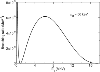
Fig. 1 shows the $d$-wave bremsstrahlung spectrum calculated for $E_{dt}$ = 50 keV. Since no resonances are present in the low-energy $\alpha$-$n$ $d$-wave scattering, the spectrum has one broad feature only. It also exhibits a sharp increase towards zero energy $E_{\gamma}$, which gives a divergent contribution to the integrated cross section. This is similar to the sharp increase of the $d+t\rightarrow\alpha+n+\gamma$ cross sections in E1 transitions, calculated in our and attributed there to unsuitability of the first-order perturbation theory at very small $E_{\gamma}$. The branching ratio, $\sigma_{dt\gamma}(E_{\gamma})/\sigma_{dt}=5.15\times 10^{-8}$ integrated above the lowest point $E_{\gamma}$ = 0.85 MeV is about three orders of magnitude smaller than the E1 value, which according to all measurement and previous theoretical calculations is around $5\times 10^{-5}$. Therefore, convection-induced transitions can be safely neglected. The same conclusion is drawn after several modifications of the intermediate channel $\alpha$-$n$ wave functions in the same fashion as described in our . The model sensitivity was not sufficiently high to warrant further investigation of this M1 path.

Refer to caption
Figure 1: The differential branching ratio $\sigma_{dt\gamma}(E_{\gamma})/\sigma_{dt}$ for convection-current-induced M1 transition for the $d$-$t$ centre-of-mass energy $E_{dt}=50$ keV.

III.2 Results for magnetization

In a sharp contrast with convection-induced M1 transition, the magnetization path turned out to be very sensitive to the model choice for the $d$-$t$ scattering wave function. The first calculation, performed here, used the potential model from Dubovichenko et al Dub19 , originally designed for a mirror scattering system, $d-^{3}$He. The $d-^{3}$He potential is represented in this model by one gaussian only, $V(r)=-V_{0}\,e^{-0.1r^{2}}$ with $V_{0}=34.5$ MeV. When applied to $d$-$t$ scattering, it gives the position of the 3/2+ resonance at about 50 keV, which is close to the experimental value. With the $d$-$t$ wave function at this energy the maximum of the M1 spectrum is also located around 16.7 MeV, but is almost twice the maximum of the E1 peak, while the integrated branching ratio, 4.1$\times 10^{-5}$, is comparable to that of the E1 transition. This is unrealistically large.

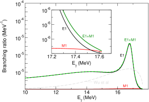
As a next step, the optical model potential from Wu et al Wu22 was used to generate the $d$-$t$ channel function. This potential is represented by a square well with a range of 3.616 fm both for the real and imaginary parts, with the corresponding real and imaginary well depths of 30 MeV and 49.64 keV, respectively. The corresponding differential branching ratio $\sigma_{dt\gamma}(E_{\gamma})/\sigma_{dt}$, also calculated at 50 keV, is compared in Fig. 2 to that obtained with the wave function from Dubovichenko et al. It is significantly smaller for $E_{\gamma}>7$ MeV, with the integrated branching ratio becoming 1.3$\times 10^{-6}$, which is only about 3$\%$ of the E1 value. However, in the area of the 17-MeV peak the M1 transition is almost half that of the E1 (see gray dashed line in Fig. 3), which still seems to be very unrealistic.

Refer to caption
Figure 2: The differential branching ratio $\sigma_{dt\gamma}(E_{\gamma})/\sigma_{dt}$ for magnetization-induced M1 transition caused obtained with three models of the $d$-$t$ wave function, described in the main text, for the $d$-$t$ centre-of-mass energy $E_{dt}=50$ keV.

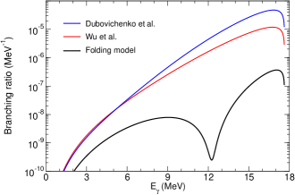
The M1 transition amplitude depends on how well the $\alpha$-$n$ and $d$-$t$ wave functions overlap in the integrand of Eq. (32). Because $\chi^{J_{i}}_{L_{dt}S_{i}L^{\prime}_{f}}(k_{i},r_{dt})$ has a node, the ${\cal I}_{L^{\prime}_{dt}\lambda^{\prime}L^{\prime}_{f}}(k_{\gamma})$ becomes very sensitive to cancellations between contributions from internal and external regions of the $d$-$t$ wave function. The potential from Dubovichenko et al has unrealistically fast (gaussian) decrease with increasing $d$-$t$ separations, while the potential from Wu et al is just a step function representing a sudden disappearance of the $d$-$t$ interaction beyond a certain point, which could have affected the strength of the M1 transition. The deuteron is a weakly bound object, so that one can expect that its interaction potential with other nuclei could be characterized by a large diffuseness. Therefore, a folding model was employed here to construct the $d$-$t$ potential at 50 keV. A simple deuteron wave function given by the HulthΓ©n model Yam54 was chosen to calculate the deuteron density, which guarantees its correct asymptotic form. The triton density was presented by a single gaussian with the range of 1.37 fm chosen to provide the triton charge radius of 1.67 fm deV87 . The nucleon-nucleon interaction is modelled by the same HulthΓ©n potential, which has a realistic rate of decrease. Then it was assumed that both the real and imaginary parts of the optical potential have the same shape. Their depths have been fitted to provide the $d$-$t$ phase shift of 16 degrees, close to the result from ab-initio calculations in Nav12 , and the reaction cross section of 4.3 b, corresponding to the astrophysical $S$-factor of 27 MeV b. With this optical folding model the calculated $\sigma_{dt\gamma}(E_{\gamma})/\sigma_{dt}$ ratio becomes 7.7$\times 10^{-5}$, which is about 1$\%$ of the E1 value integrated above $E_{\gamma}=10$ MeV. The differential branching ratios from all three $d$-$t$ interaction models are compared to each other in Fig. 2. The minimum around 12 MeV in the folding model calculation is due to the almost complete cancellation between internal and external contributions from the $d$-$t$ wave function at this point. In Fig. 3 the M1 contribution calculated in the present optical folding model is compared to the E1 contribution from our . It gives about 2$\%$ at the main peak but is negligible everywhere below 15 MeV. It starts to dominate the E1 transition above $E_{\gamma}\gtrsim 17.5$ MeV leading to additional counts in the $\gamma$-spectrum in this area, which potentially could be mistaken for background.

Refer to caption
Figure 3: The differential branching ratio $\sigma_{dt\gamma}(E_{\gamma})/\sigma_{dt}$ for magnetization-induced M1 transition, calculated at $E_{dt}=50$ keV with optical folding model $d$-$t$ potential from this work, in comparison to the E1 contribution from our . The grey dashed line represents M1 calculation with optical model $d$-$t$ potential of Wu et al.

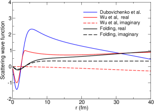
To understand the difference between the three model calculations the wave functions from gaussian model of Dubovichenko et al, square well optical model of Wu et al and the present optical folding model are compared to each other in Fig. 4. It is noticeable that the folding model wave function spreads out much further, with the node at a significantly larger $d$-$t$ separation. This leads to a smaller absolute values of the wave function as compared to Dubovichenko et and and Wu et al, which is responsible for the small M1 contribution.

Refer to caption
Figure 4: The $d$-$t$ scattering wave function at $E_{dt}=50$ keV calculated with gaussian potential from Dubovichenko et al, square well optical model from Wu et al and the optical folding model of the present paper.

IV Discussion and conclusions

The present study of the M1 contribution to the $d+t\rightarrow\alpha+n+\gamma$ cross section shows that it is dominated by the direct transition from the $s$-wave $d$-$t$ partition of 5He to the $s$-wave $\alpha$-$n$ partition in the final channel. The corresponding cross section has been found to be strongly dependent on the model choice for the $d$-$t$ scattering wave function. In particular, it depends on how fast the $d$-$t$ interaction potential decreases with the $d$-$t$ separation. With the choice of two potential models from the literature, one having a gaussian decrease and another one being just a square well, the M1 transition becomes unrealistically large due to the large values of $d$-$t$ channel function inside the $d$-$t$ interaction. The optical folding potential, constructed in this work, provides a more spatially extended $d$-$t$ interaction, which leads to a further spread and the correspondingly smaller values of the $d$-$t$ wave function within the $d$-$t$ interaction region. This leads to a much smaller M1 cross section.

The strong model dependence of the M1 transition is reminiscent of the situation with theoretical calculations of $\beta$-delayed deuteron emission 6He $\rightarrow\alpha+d+e^{-}+\bar{\nu}_{e}$. Its measured branching ratio to the main 6Li ground state decay branch is very small, of the order of 10-6, however, potential model predictions are two orders of magnitude higher Bor93 . To bring theoretical predictions down, full three-body calculations of both the 6He $=\alpha+n+n$ and 6Li $=\alpha+n+p$ must be performed Tur06 ; Tur18 , keeping all the quantum numbers included. Such a situation is due to the spatial parts of 6He and $\alpha+d$ wave functions being almost orthogonal, which could be achieved in full calculations only.

The operator $\sum_{i}\sigma_{i}t_{3i}$ that causes the Galow-Teller transition 6He $\rightarrow\alpha+d+e^{-}+\bar{\nu}_{e}$ is almost identical to the M1 operator of this paper if the long-wave approximation is done. Although all results for $d+t\rightarrow\alpha+n+\gamma$ shown here do not use the long-wave approximation, it has been checked numerically that this approximation does not change much the results. A similarity with the $\beta$-delayed deuteron emission of 6He is also in the three-body nature of the $d$-$t$ system, which could be considered as a strongly-bound triton plus neutron plus proton. The lessons learned from $\beta$-decay studies tell us that for reliable calculations of the M1 transition one has to go beyond the two-body potential model description of the $d$-$t$ motion and include into consideration such details as deuteron breakup and polarization in the sub-Coulomb $d$-$t$ scattering. Also, more quantum numbers, such as the $d$-wave state admixture in the incoming deuteron, should be included in the calculations.

This work has been motivated by a possibility of having more counts near the endpoint of the $\gamma$-spectrum from $d$-$t$ collisions due to M1 transition to the final near-zero energy $s$-wave $\alpha$-$n$ state, which could be favored because of the absence of the centrifugal barrier. A realistic model of the $d$-$t$ interaction suggests that the strength of the spectrum in this area is about 2$\%$ only, which would not induce much of a systematical error in the background subtraction. However, to confirm this conclusion, as a minimum, three-body treatment of the $d$-$t$ collisions are required. In the long term, five-body calculations starting from realistic nucleon-nucleon interactions will be needed to clarify this matter.

Acknowledgements.
This work was part-funded by AWE, UK Ministry of Defence Β©Crown owned copyright 2024/AWE. Remaining part of funding came from the United Kingdom Science and Technology Facilities Council (STFC) under Grant No. ST/V001108/1.

V Appendix

V.1 Matrix element of $\vec{L}\phi_{\lambda\mu}\cdot\vec{\nabla}$

To develop a formal expression for M1 amplitude given by Eq. (23) one needs the following matrix element:

$\displaystyle\langle l_{f}m_{f}\mid\vec{L}\phi_{\lambda\mu}\cdot\vec{\nabla}\mid l_{i}m_{i}\rangle=\langle l_{f}m_{f}\mid\vec{L}\phi_{\lambda\mu}\cdot\vec{n}\mid l_{i}m_{i}\rangle\frac{\partial}{\partial r}$
$\displaystyle+\,\langle l_{f}m_{f}\mid\vec{L}\phi_{\lambda\mu}\cdot\vec{\nabla}_{\Omega}\mid l_{i}m_{i}\rangle\frac{1}{r}.\,\,\,\,\,\,\,\,\,\,\,\,\,\,\,\,\,\,\,\,$ (37)

Using

$\displaystyle L_{\nu}\phi_{\lambda\mu}=\sqrt{\lambda(\lambda+1)}\,j_{\lambda}(kr)\sum_{\mu^{\prime}}(\lambda\mu 1\nu|\lambda\mu^{\prime})Y_{\lambda\mu^{\prime}}(\hat{\mbox{\boldmath$r$}})\,\,\,\,\,\,\,\,\,\,\,\,\,\,\,\,$ (38)

and

$\displaystyle\langle l_{f}m_{f}\mid\vec{\nabla}_{\Omega}\mid l_{i}m_{i}\rangle=(l_{i}m_{i}\lambda\mu|l_{f}m_{f})\hat{l}^{-1}_{f}{\cal C}_{l_{i}l_{f}},$ (39)
$\displaystyle{\cal C}_{l_{i}l_{f}}=-\left(l_{i}\sqrt{l_{i}+1}\delta_{l_{f},l_{i}+1}+(l_{i}+1)\sqrt{l_{i}}\delta_{l_{f},l_{i}-1}\right),\,\,\,\,\,\,\,\,\,\,\,$ (40)

one obtains

$\displaystyle\langle l_{f}m_{f}\mid\vec{L}\phi_{\lambda\mu}\cdot\vec{\nabla}\mid l_{i}m_{i}\rangle=\hat{\lambda}\,(l_{i}m_{i}\lambda\mu|l_{f}m_{f})$
$\displaystyle\times\frac{1}{\sqrt{4\pi}}j_{\lambda}(kr)\left({\cal D}^{(1)}_{l_{i}\lambda l_{f}}\frac{\partial}{\partial r}+{\cal D}^{(2)}_{l_{i}\lambda l_{f}}\frac{1}{r}\right),$ (41)

where

$\displaystyle{\cal D}^{(1)}_{l_{i}\lambda l_{f}}=(-)^{\lambda}\sqrt{\lambda(\lambda+1)}\sum_{L}(L010|l_{i}0)$
$\displaystyle\times(l_{f}0\lambda 0|L0)W(l_{i}1l_{f}\lambda;L\lambda)$ (42)

and

$\displaystyle{\cal D}^{(2)}_{l_{i}\lambda l_{f}}=(-)^{\lambda+1}\sqrt{\lambda(\lambda+1)(2\lambda+1)}\,\,$
$\displaystyle\times\sum_{L}{\cal C}_{l_{i}L}(l_{f}0\lambda 0|L0)W(l_{i}1l_{f}\lambda;L\lambda).$ (43)

V.2 Spin and isospin matrix elements

The contribution from nucleons inside the triton is characterized by $e^{i\vec{k}_{\gamma}\vec{r}_{j}}$. The coordinate of each nucleon is $\vec{r}_{j}=\vec{r}^{\prime}_{j}-\vec{r}_{t}$, where $\vec{r}^{\prime}_{j}$ is its position with respect to the triton centre of mass and $\vec{r}_{t}=-\tfrac{2}{5}\vec{r}_{dt}$ is the position of the latter with respect to the 5He centre of mass. Because triton is spatially confined one can assume that $e^{i\vec{k}_{\gamma}\vec{r}_{j}}\approx 1$. In this approximation the M1 magnetization-induced amplitude does not contain spatial variables and, therefore, one has to consider matrix elements in the spin space only. There are three such matrix elements, the first of which is

$\displaystyle\sum_{i=1,2,3}\langle\psi_{t}(1,2,3)\mid S_{\mu,i}g_{s_{i}}\mid\psi_{t}(1,2,3)\rangle\,\,\,\,\,\,\,\,\,\,\,\,\,\,\,\,\,\,\,\,\,\,\,\,\,\,\,\,\,\,\,\,\,\,\,\,$
$\displaystyle=\frac{1}{2}(g_{n}+g_{p})\langle\psi_{t}\mid S_{\mu}\mid\psi_{t}\rangle\,\,\,\,\,\,\,\,\,\,\,\,\,\,$
$\displaystyle+\,(g_{n}-g_{p})\sum_{i=1,2,3}\langle\psi_{t}(1,2,3)\mid S_{\mu,i}t_{3i}\mid\psi_{t}(1,2,3)\rangle\,\,\,\,\,\,\,\,\,\,\,\,$ (44)

To evaluate the second term it is assumed here that the triton wave functions is dominated by the fully antisymmetric in spin-isospin space component $\left|[3]S=\mbox{$\frac{1}{2}$}M_{S}T=\mbox{$\frac{1}{2}$}M_{T}\right.\rangle$ described by the Young’s tableau $[f]=[3]$ with spin and isospin equal to 1/2 and the spin and isospin projections of $M_{S}$ and $M_{T}$, respectively. Using fractional parentage expansion to extract the $m$-th nucleon from this spin-isospin component:

$\displaystyle\mid[3]S=\mbox{$\frac{1}{2}$}M_{S}T=\mbox{$\frac{1}{2}$}M_{T}\rangle=$
$\displaystyle\sum_{[f_{2}]S_{2}T_{2}M_{2}M_{T_{2}}}\langle[3]\mbox{$\frac{1}{2}$}\mbox{$\frac{1}{2}$}\mid[f_{2}]S_{2}T_{2}\rangle\mid[f_{2}]S_{2}M_{2}T_{2}M_{T_{2}}\rangle$
$\displaystyle\times(S_{2}M_{2}\mbox{$\frac{1}{2}$}\sigma|\mbox{$\frac{1}{2}$}M_{S})(T_{2}M_{T_{2}}\mbox{$\frac{1}{2}$}\tau|\mbox{$\frac{1}{2}$}M_{T})\chi^{\rm spin}_{\mbox{$\frac{1}{2}$}\sigma}(m)\chi^{\rm isopin}_{\mbox{$\frac{1}{2}$}\tau}(m),$
(45)

where $\langle[3]\mbox{$\frac{1}{2}$}\mbox{$\frac{1}{2}$}\mid[f_{2}]S_{2}T_{2}\rangle$ is the fractional parentage expansion coefficient and $\mid[f_{2}]S_{2}M_{2}T_{2}M_{T_{2}}\rangle$ is the two-body spin-isospin function, and then performing all summations over spin and isospin projections, one obtains

$\displaystyle\langle[3]\mbox{$\frac{1}{2}$}M^{\prime}_{S}\mbox{$\frac{1}{2}$}M^{\prime}_{T}\mid\sum_{i=1,2,3}S_{\mu,i}t_{3i}\mid[3]\mbox{$\frac{1}{2}$}M_{S}\mbox{$\frac{1}{2}$}M_{T}\rangle$
$\displaystyle=3\langle[3]\mbox{$\frac{1}{2}$}M^{\prime}_{S}\mbox{$\frac{1}{2}$}M^{\prime}_{T}\mid S_{\mu,m}t_{3m}\mid[3]\mbox{$\frac{1}{2}$}M_{S}\mbox{$\frac{1}{2}$}M_{T}\rangle$
$\displaystyle=M_{T}\delta_{M_{T}M^{\prime}_{T}}\langle\psi_{t}|S_{\mu}|\psi_{t}\rangle.\,\,\,\,\,\,\,\,\,\,\,\,\,\,\,\,\,\,\,\,\,\,\,\,\,\,\,$ (46)

Therefore, for the isospin projection $M_{T}=1/2$, associated with triton,

$\displaystyle\sum_{i=1,2,3}\langle\psi_{t}(1,2,3)\mid S_{\mu,i}g_{s_{i}}\mid\psi_{t}(1,2,3)\rangle=$
$\displaystyle=g_{n}\langle\psi_{t}|S_{\mu}|\psi_{t}\rangle=\frac{1}{\sqrt{2}}g_{n}(\mbox{$\frac{1}{2}$}M^{\prime}_{t}1\mu|\mbox{$\frac{1}{2}$}M_{t})\langle\mbox{$\frac{1}{2}$}||\mbox{\boldmath$S$}||\mbox{$\frac{1}{2}$}\rangle.\,\,\,\,\,\,\,\,\,\,\,\,$ (47)

Then, supplementing the triton wave function with spin functions of theremaining neuton and proton, one has

$\displaystyle\langle[[\psi_{t}\otimes\chi^{\rm spin}_{\mbox{$\frac{1}{2}$}}(p)]_{0}\otimes\chi^{\rm spin}_{\mbox{$\frac{1}{2}$}}(n)]_{\mbox{$\frac{1}{2}$}\sigma_{n}}|\sum_{i=1,2,3}{S}_{\mu,i}g_{si}$
$\displaystyle\times\,|\chi^{\rm spin}_{\mbox{$\frac{1}{2}$}}[\psi_{t}\otimes\chi^{\rm spin}_{1}(p,n)]_{S_{i}M_{S_{i}}}\rangle$
$\displaystyle=g_{n}\frac{1}{\sqrt{2}}(1\mu S_{i}M_{S_{i}}|\mbox{$\frac{1}{2}$}\sigma_{n}).\,\,\,\,\,\,\,\,\,\,\,\,\,\,\,\,\,\,\,\,\,\,\,\,$ (48)

For $i=4$, which is a proton in deuteron, the spin part is simpler,

$\displaystyle\langle[[\psi_{t}\otimes\chi^{\rm spin}_{\mbox{$\frac{1}{2}$}}(p)]_{0}\otimes\chi^{\rm spin}_{\mbox{$\frac{1}{2}$}}(n)]_{\mbox{$\frac{1}{2}$}\sigma_{n}}|{S}_{\mu}(p)g_{sp}$
$\displaystyle\times|[\psi_{t}\otimes\chi^{\rm spin}_{1}(p,n)]_{S_{i}M_{S_{i}}}\rangle=g_{p}\sqrt{\frac{1}{2}}(1\mu S_{i}M_{S_{i}}|\mbox{$\frac{1}{2}$}\sigma_{n}),\,\,\,\,\,\,\,\,\,\,\,\,$ (49)

which is exactly the same as in the case of $i=1,2,3$ except for the neutron gyromagnetic factor $g_{n}$ being replaced by the the proton gyromagnetic factor $g_{p}$.

For $i=5$, which is a neutron in deuteron, the spin matrix element is

$\displaystyle\langle[[\psi_{t}\otimes\chi^{\rm spin}_{\mbox{$\frac{1}{2}$}}(p)]_{0}\otimes\chi^{\rm spin}_{\mbox{$\frac{1}{2}$}}(n)]_{\mbox{$\frac{1}{2}$}\sigma_{n}}|{S}_{\mu}(n)g_{sn}$
$\displaystyle\times|[\psi_{t}\otimes\chi^{\rm spin}_{1}(p,n)]_{S_{i}M_{S_{i}}}\rangle$
$\displaystyle=W(\mbox{$\frac{1}{2}$}\mbox{$\frac{1}{2}$}S_{i};01)\frac{1}{2}\langle\mbox{$\frac{1}{2}$}||\vec{S}||\mbox{$\frac{1}{2}$}\rangle(\mbox{$\frac{1}{2}$}M_{S_{i}}1\mu|\mbox{$\frac{1}{2}$}\sigma_{n_{f}}),$ (50)

which is non-zero only for $S_{i}=1/2$. Given that the M1 transitions considered in this paper come from the resonance component with spin $S_{i}=3/2$, the contribution from nucleon 5 (which is the neutron in deuteron) is set to zero.

Finally, the matrix elements (48) and (49) should be further multiplied by the isospin part of the M1 matrix element, which is

$\displaystyle\langle\chi^{\rm isospin}_{\mbox{$\frac{1}{2}$}\mbox{$\frac{1}{2}$}}(1,2,3)\chi^{\rm isospin}_{\mbox{$\frac{1}{2}$}-\mbox{$\frac{1}{2}$}}(4)\chi^{\rm isospin}_{\mbox{$\frac{1}{2}$}\mbox{$\frac{1}{2}$}}(n)\,\,\,\,\,\,\,\,\,\,\,\,\,\,\,\,\,\,\,\,\,\,\,\,\,\,\,\,\,\,\,\,\,$
$\displaystyle\times\,|\chi^{\rm isospin}_{\mbox{$\frac{1}{2}$}\mbox{$\frac{1}{2}$}}(1,2,3)\chi^{\rm isospin}_{00}(p,n)\rangle=(\mbox{$\frac{1}{2}$}-\mbox{$\frac{1}{2}$}\mbox{$\frac{1}{2}$}\mbox{$\frac{1}{2}$}|00)$
$\displaystyle=-\frac{1}{\sqrt{2}}.\,\,\,\,\,\,\,\,\,\,\,\,\,\,\,\,\,\,\,\,$ (51)

V.3 Spatial matrix element for M1 magnetization amplitude

The calculate the M1 amplitude the integration should be performed either over $d\vec{r}_{\alpha n}d\vec{r}_{pt}$ or over $d\vec{r}_{np}d\vec{r}_{dt}$. This task is simplified if integration is performed over $d\vec{r}_{\alpha n}d\vec{r}_{dt}$ - the variables of the continuum state wave functions. Because $\vec{r}_{tp}=\tfrac{8}{5}\vec{r}_{dt}-\tfrac{4}{5}\vec{r}_{\alpha n}$ and $\vec{r}_{np}=\tfrac{8}{5}\vec{r}_{\alpha n}-\tfrac{6}{5}\vec{r}_{dt}$, one has $d\vec{r}_{\alpha n}d\vec{r}_{pt}=\left(\tfrac{8}{5}\right)^{3}\vec{r}_{\alpha n}d\vec{r}_{dt}$. Then the product of the radial parts of the overlap $I_{pt}$ and the deuteron wave function $\psi_{d}$ could be represented as

$\displaystyle I_{pt}({r}_{pt})\varphi_{d}({r}_{np})$ $\displaystyle=$ $\displaystyle 4\pi\sum_{lm}{\cal F}_{l}(r_{dt},r_{\alpha n})Y^{*}_{lm}(\hat{\mbox{\boldmath$r$}}_{dt})Y_{lm}(\hat{\mbox{\boldmath$r$}}_{\alpha n}),$
$\displaystyle{\cal F}_{l}(r_{dt},r_{\alpha n})$ $\displaystyle=$ $\displaystyle\frac{1}{2}\int_{-1}^{1}d\mu\,P_{\lambda}(\mu)\varphi_{d}\left(|\tfrac{6}{5}\mbox{\boldmath$r$}_{dt}-\tfrac{8}{5}\mbox{\boldmath$r$}_{\alpha n}|\right)$ (52)
$\displaystyle\times$ $\displaystyle I_{pt}(|\tfrac{8}{5}\mbox{\boldmath$r$}_{dt}-\tfrac{4}{5}\mbox{\boldmath$r$}_{\alpha n}|).$

Using the results for both spin and isospin matrix elements derived in the subsection above, one can obtain that the M1 amplitude contains the matrix element over the angular variables

$\displaystyle F=-i\sum_{lm}{\cal F}_{l}(r_{dt},r_{\alpha n})\langle Y_{L^{\prime}_{f}M^{\prime}_{f}}(\hat{\mbox{\boldmath$r$}}_{\alpha n})Y_{lm}(\hat{\mbox{\boldmath$r$}}_{dt})\mid g_{n}\left[\vec{\nabla}_{t}\times\vec{L}_{t}\phi_{\lambda\mu}(r_{t})\right]_{\nu}+g_{p}\left[\vec{\nabla}_{p}\times\vec{L}_{p}\phi_{\lambda\mu}(r_{p})\right]_{\nu}\mid Y_{L^{\prime}_{dt}M^{\prime}_{dt}}(\hat{\mbox{\boldmath$r$}}_{dt})Y_{lm}(\hat{\mbox{\boldmath$r$}}_{\alpha n})\rangle.$
(53)

The first term is further developed using

$\displaystyle\langle Y_{lm}(\hat{\mbox{\boldmath$r$}}_{dt})\mid\left[\vec{\nabla}_{t}\times\vec{L}_{t}\phi_{\lambda\mu}(r_{t})\right]_{\nu}\mid Y_{L^{\prime}_{dt}M^{\prime}_{dt}}(\hat{\mbox{\boldmath$r$}}_{dt})\rangle$
$\displaystyle=k\sum_{\lambda^{\prime}\mu^{\prime}}(-)^{\lambda^{\prime}}c_{\lambda\lambda^{\prime}}(\lambda\mu 1\nu|\lambda^{\prime}\mu^{\prime})j_{\lambda^{\prime}}(\tfrac{2}{5}k_{\gamma}r_{dt})$
$\displaystyle\times\,(L^{\prime}_{dt}0\lambda^{\prime}0|L^{\prime}_{f}0)\frac{\hat{L}^{\prime}_{dt}\hat{\lambda}^{\prime}}{\sqrt{4\pi}\hat{L}^{\prime}_{f}}\,\,\,\,\,\,\,\,\,\,\,\,\,\,\,\,\,\,$ (54)

with

$\displaystyle c_{\lambda\lambda^{\prime}}$ $\displaystyle=$ $\displaystyle-(\lambda+1)\sqrt{\frac{\lambda}{2\lambda-1}},\,\,\,\,\,\,\,\,\lambda^{\prime}=\lambda-1$ (55)
$\displaystyle 0\,\,\,\,\,\,\,\,\,\,\,\,\,\,\,\,\,\,\,\,\,\,\,\,\,\,\,\,\,\,\,\,\,\,\,\,\,\,\,\,\,\,\,\,\,\,\,\,\,\,\,\,\,\,\,\,\,\lambda^{\prime}=\lambda$
$\displaystyle\lambda\sqrt{\frac{\lambda+1}{2\lambda+3}},\,\,\,\,\,\,\,\,\,\,\,\,\,\,\,\,\,\,\,\,\,\,\,\,\,\,\,\,\,\lambda^{\prime}=\lambda+1.$

To develop the second term of (53), one has to use a general expansion for $\mbox{\boldmath$r$}=\alpha_{1}\mbox{\boldmath$r$}_{1}+\alpha_{2}\mbox{\boldmath$r$}_{2}$

$\displaystyle-i\left[\vec{\nabla}\times\vec{L}\phi_{\lambda\mu}(r)\right]_{\nu}=\sqrt{4\pi}k\sum_{\lambda^{\prime}\mu^{\prime}\lambda_{1}\lambda_{2}\mu_{1}\mu_{2}}i^{-\lambda_{1}+\lambda_{2}-\lambda^{\prime}}c_{\lambda\lambda^{\prime}}$
$\displaystyle\times(\lambda_{1}0\lambda_{2}0|\lambda^{\prime}0)j_{\lambda_{1}}(\alpha_{1}kr_{1})j_{\lambda_{2}}(\alpha_{2}kr_{2})$
$\displaystyle\times(\lambda_{1}\mu_{1}\lambda^{\prime}\mu^{\prime}|\lambda_{2}\mu_{2})(\lambda\mu 1\nu|\lambda^{\prime}\mu)Y^{*}_{\lambda_{1}\mu_{1}}(\hat{\mbox{\boldmath$r$}}_{1})Y_{\lambda_{2}\mu_{2}}(\hat{\mbox{\boldmath$r$}}_{2})$
(56)

In the case of $\mbox{\boldmath$r$}_{p}=\tfrac{6}{5}\mbox{\boldmath$r$}_{dt}-\tfrac{4}{5}\mbox{\boldmath$r$}_{\alpha n}$ the final result for $F$ becomes

$\displaystyle F$ $\displaystyle=$ $\displaystyle k\frac{\hat{L}^{\prime}_{dt}}{\sqrt{4\pi}}\sum_{\lambda^{\prime}\mu^{\prime}}c_{\lambda\lambda^{\prime}}F_{L^{\prime}_{dt}\lambda^{\prime}L^{\prime}_{f}}(r_{dt},r_{\alpha n})$ (57)
$\displaystyle\times$ $\displaystyle(\lambda\mu 1\nu|\lambda^{\prime}\mu^{\prime})(\lambda^{\prime}\mu^{\prime}L^{\prime}_{dt}M^{\prime}_{dt}|L^{\prime}_{f}M^{\prime}_{f}),$

where

$\displaystyle F_{L^{\prime}_{dt}\lambda^{\prime}L^{\prime}_{f}}(r_{dt},r_{\alpha n})=g_{p}{\cal G}_{L^{\prime}_{dt}\lambda^{\prime}L^{\prime}_{f}}(r_{dt},r_{\alpha n})\,\,\,\,\,\,\,\,$
$\displaystyle+\,g_{n}(L^{\prime}_{dt}0\lambda^{\prime}0|L^{\prime}_{f}0)j_{\lambda^{\prime}}(\tfrac{2}{5}kr_{dt}){\cal F}_{L^{\prime}_{f}}(r_{dt},r_{\alpha n})$ (58)

with

$\displaystyle{\cal G}_{L^{\prime}_{dt}\lambda^{\prime}L^{\prime}_{f}}(r_{dt},r_{\alpha n})=\sum_{\lambda_{1}\lambda_{2}l}{\cal C}_{\lambda_{1}\lambda_{2}l}{\cal F}_{l}(r_{dt},r_{\alpha n})$
$\displaystyle\times j_{\lambda_{1}}(\tfrac{6}{5}kr_{dt})j_{\lambda_{2}}(\tfrac{4}{5}kr_{\alpha n})$ (59)

and

$\displaystyle{\cal C}_{\lambda_{1}\lambda_{2}l}=\sum_{\lambda_{1}\lambda_{2}}i^{\lambda_{1}+\lambda_{2}-\lambda^{\prime}}\hat{\lambda}^{2}_{1}\hat{\lambda}^{2}_{2}(\lambda_{1}0L^{\prime}_{dt}0|l0)$
$\displaystyle\times(\lambda_{2}0L^{\prime}_{f}0|l0)(\lambda_{1}0\lambda_{2}0|\lambda^{\prime}0)W(\lambda^{\prime}\lambda_{1}L^{\prime}_{f}l;\lambda_{2}L^{\prime}_{dt}).$ (60)

Then standard algebra manipulations lead to (31) and (32).

V.4 Exchange contribution to magnetization

The simplest way to calculate the exchange contribution

$\displaystyle\langle\Phi^{(41)}_{\alpha n,M_{n}}(1,2,3,4;5)\mid{\cal M}^{M\lambda}_{\mu}\mid\Phi^{(32)}_{dt,M_{d}M_{t}}(3,4,5;1,2)\rangle$

to the M1 amplitude is to use the long-wave approximation, justified by smallvalues of the $k_{\gamma}r$ contributing to the process. In this approximation, one has to deals with matrix elements of the operator $\sum_{i}g_{si}S_{\mu,i}=(g_{n}+g_{p})\sum_{i}S_{\mu,i}+(g_{n}-g_{p})\sum_{i}S_{\mu,i}t_{3i}$. This could be achieved by making fractional parentage decomposition of the $\alpha$-particle wave function in the exit channel into the product of two deuteron wave functions keeping only the terms corresponding to the deuteron ground state wave function,

$\displaystyle\psi_{\alpha}(1,2,3,4)\approx\left[\psi_{d}(1,2)\times\psi_{d}(3,4)\right]_{00}I_{dd}(\vec{r}_{dd}),$ (61)

with the isospin Clebsch-Gordon coefficient embedded in the overlap function $I_{dd}(\vec{r}_{dd})$. The triton wave function in the initial state is also expanded as

$\displaystyle\psi_{t}(3,4,5)$ $\displaystyle=$ $\displaystyle I_{nd}(\vec{r}_{nd})\varphi_{d}(\vec{r}_{34})[\chi^{\rm spin}_{1}(3,4)\chi^{\rm spin}_{\mbox{$\frac{1}{2}$}}(5)]_{J_{t}M_{t}}$ (62)

Then considering only the $s$-wave components in the deuteron wave functions and overlaps one has to calculate the matrix element

$\displaystyle\langle[\chi^{\rm spin}_{1}(1,2)\times\chi^{\rm spin}_{1}(3,4)]_{00}\,\chi^{\rm spin}_{\sigma_{n_{f}}}(5)X^{\rm isospin}\mid\sum_{i=1}^{5}S_{\mu,i}g_{s_{i}}\mid[[\chi^{\rm spin}_{1}(3,4)\times\chi^{\rm spin}_{\mbox{$\frac{1}{2}$}}(5)]_{J_{t}}\times\chi^{\rm spin}_{1}(1,2)]_{S_{i}M_{S_{i}}}X^{\rm isospin}\rangle,\,\,\,\,\,$ (63)

where $X^{\rm isospin}$is the isospin part of the five-body system. It is easy to show that

$\displaystyle\sum_{i=1,2}\langle\chi^{\rm spin}_{1M^{\prime}_{d}}(1,2)\chi^{\rm isospin}_{00}(1,2)\mid S_{\mu,i}t_{3i}\mid\chi^{\rm spin}_{1M_{d}}(1,2)\chi^{\rm isospin}_{00}(1,2)\rangle=0$ (64)

and

$\displaystyle\sum_{i=1,2}\langle\chi^{\rm spin}_{1M^{\prime}_{d}}(1,2)\chi^{\rm isospin}_{00}(1,2)\mid S_{\mu,i}\mid\chi^{\rm spin}_{1M_{d}}(1,2)\chi^{\rm isospin}_{00}(1,2)\rangle=-\sqrt{2}(1\mu 1M_{d}|1M^{\prime}_{d}).$ (65)

The same is true for nucleons 3 and 4. Also,

$\displaystyle\langle\chi^{\rm spin}_{\mbox{$\frac{1}{2}$}\sigma^{\prime}_{5}}(5)\chi^{\rm isospin}_{\mbox{$\frac{1}{2}$},\mbox{$\frac{1}{2}$}}(5)\mid S_{\mu}g_{s_{5}}\mid\chi^{\rm spin}_{\mbox{$\frac{1}{2}$}\sigma_{5}}(5)\chi^{\rm isospin}_{\mbox{$\frac{1}{2}$},\mbox{$\frac{1}{2}$}}(5)\rangle=g_{n}(\mbox{$\frac{1}{2}$}\sigma_{5}1\mu|\mbox{$\frac{1}{2}$}\sigma^{\prime}_{5})\frac{1}{\sqrt{2}}\langle\mbox{$\frac{1}{2}$}||S||\mbox{$\frac{1}{2}$}\rangle$ (66)

Then, after further algebraic manipulations, one obtains that the spin-isospin latrix element (63) is equal to

$\displaystyle\frac{1}{2}(g_{n}+g_{p})(\mbox{$\frac{1}{2}$}M_{S_{i}}1\mu|\mbox{$\frac{1}{2}$}\sigma_{n_{f}})\sum_{S}(-)^{S+S_{i}}\hat{S}_{i}\hat{S}W(11\mbox{$\frac{1}{2}$}S;1S_{i})\left[(-)^{J_{t}+1-S_{i}}\delta_{SJ_{t}}+(-)^{3/2-S}\hat{S}\hat{J}_{t}W(1\mbox{$\frac{1}{2}$}S_{i}1;SJ_{t})\right]$
$\displaystyle+(-)^{J_{t}+1-S_{i}}g_{n}W(11S_{i}\mbox{$\frac{1}{2}$};0J_{t})\hat{J}_{t}(\mbox{$\frac{1}{2}$}M_{S_{i}}1\mu|\mbox{$\frac{1}{2}$}\sigma_{n_{f}})\,\,\,\,\,\,\,\,\,\,\,\,\,\,\,\,\,\,\,\,\,\,\,\,\,\,\,\,\,\,$ (67)

For $S_{i}=3/2$ and $J_{t}=1/2$ it is equal to zero.

References

  • (1) M.J. Moran and B. Chang, MOLE: A new high-energy gamma-ray diagnostic. United States: N. p., 1992. Web. doi:10.2172/5656147
  • (2) W. Buss, H. WΓ€qffler, and B. Ziegler, Radiative capture of deuterons by 3H, Physics Letters 4, 198 (1963).
  • (3) A. Kosiara and H. Willard, Phys. Lett. 15, B 32, 99 (1970).
  • (4) V. M. Bezotosnyi, V. A. Zhmailo, L. M. Surov, and M. S.Shvetsov, Sov. J. Nucl. Phys. 10, 127 (1970).
  • (5) F. E. Cecil and F. J. Wilkinson, Phys. Rev. Lett. 53, 767 (1984).
  • (6) G. L. Morgan, P. W. Lisowski, S. A. Wender, R. E. Brown, N. Jarmie, J. F. Wilkerson, and D. M. Drake, Phys. Rev. C 33, 1224 (1986).
  • (7) J. E. Kammeraad, J. Hall, K. E. Sale, C. A. Barnes, S. E. Kellogg, and T. R. Wang, Phys. Rev. C 47, 29 (1993).
  • (8) Y. Kim et al, Phys. Rev. C 85, 061601 (2012).
  • (9) J. Jeet, A. B. Zylstra, M. Rubery, Y. Kim, K. D. Meaney, C. Forrest, V. Glebov, C. J. Horsfield, A. M. McEvoy, and H. W. Herrmann, Phys. Rev. C 104, 054611 (2021).
  • (10) K. D. Meaney, Y. Kim, H. Geppert-Kleinrath, H. W. Herrmann, A. S. Moore, E. P. Hartouni, D. J. Schloss- berg, E. Mariscal, J. Carrera, and J. A. Church, Phys. Plasmas 28, 102702 (2021)
  • (11) Z. Mohamed, Y. Kim, and J. Knauer, Front. Phys. 10, 10.3389/fphy.2022.944339 (2022).
  • (12) Z. L. Mohamed, Y. Kim, J. P. Knauer, and M. S. Rubery, Phys. Rev. C 107, 014606 (2023).
  • (13) K. D. Meaney, M. W. Paris, G. M. Hale, Y. Kim, J. Kuczek, and A. C. Hayes, Phys. Rev. C 109, 034003 (2024)
  • (14) A. Dal Molin, G. Marcer, M. Nocente, M. Rebai, D. Rigamonti, M. Angelone, A. Bracco, F. Camera, C. Cazzaniga, T. Craciunescu, G. Croci, M. Dalla Rosa, L. Giacomelli, G. Gorini, Y. Kazakov, E.M. Khilkevitch, A. Muraro, E. Panontin, E. Perelli Cippo, M. Pillon, O. Putignano, J. Scionti, A. E. Shevelev, A. Ε½ohar, and M. Tardocchi, Phys. Rev. Lett. 133, 055102 (2024)
  • (15) M. Rebai, D. Rigamonti, A. Dal Molin, G. Marcer, A. Bracco, F. Camera, D. Farina, G. Gorini, E. Khilkevitch, M. Nocente, E. P. Cippo, O.r Putignano, J. Scionti, A. Shevelev, A. Zohar, and M. Tardocchi, Phys. Rev. C 110, 014625 (2024)
  • (16) C. J. Horsfield, M. S. Rubery, J. M. Mack, H. W. Herrmann, Y. Kim, C. S. Young, S. E. Caldwell, S. C. Evans, T. S. Sedillo, A. M. McEvoy, N. M. Hoffman, M. A. Huff, J. R. Langenbrunner, G. M. Hale, D. C. Wilson, W. Stoeffl, J. A. Church, E. M. Grafil, E. K. Miller, and V. Yu Glebov Phys. Rev. C 104, 024610 (2021)
  • (17) N.K. Timofeyuk, G.W. Bailey and M.R. Gilbert, Phys. Rev. C 110, 014612 (2024)
  • (18) D.Baye, Phys. Rev. C 86, 034306 (2012)
  • (19) D. Baye and P. Descouvemont, Nucl. Phys. A 443, 302 (1985)
  • (20) J. Dohet-Eraly and D. Baye, Phys. Rev. C 88, 024602 (2013)
  • (21) G.R. Satchler, L.W. Owen, A.J. Elwyn, G.L. Morgan and R.L. Walter, Nucl. Phys. A 112, 1 (1968)
  • (22) H. Fiedeldey, Nucl. Phys. A 77, 149 (1966)
  • (23) P. NavrΓ‘til and S. Quaglioni, Phys. Rev. Lett. 108, 042503 (2012).
  • (24) S.B. Dubovichenko and N.A. Burkova and A.V. Dzhazairov-Kakhramanov and R.Ya. Kezerashvili and Ch.T. Omarov and A.S. Tkachenko and D.M. Zazulin, Nucl. Phys. A 987, 46 (2019)
  • (25) B.Wu, H.Duan, J.Liu Nucl. Phys. A 1017, 122340 (2022)
  • (26) Y. Yamaguchi, Phys Rev. 95, 1628 (1954)
  • (27) H. De Vries, C. W. De Jager, and C. De Vries, At. Data and Nucl. Data Tables, 36 (1987) 495 (1987)
  • (28) M. J. G. Borge, L. Johannsen, B. Jonson, T. Nilsson, G. Nyman, K. Riisager, O. Tengblad, and K. Wilhelmsen Rolander, Nucl. Phys. A 560, 664 (1993).
  • (29) E.M. Tursunov, D. Baye and P. Descouvemont, Phys.Rev. C 73, 014303 (2006); Erratum Phys.Rev. C 74, 069904 (2006)
  • (30) E.M. Tursunov, D. Baye and P. Descouvemont, Phys.Rev. C 97, 014302 (2018)