Limiting Spectral Distribution of a Random Commutator Matrix

Abstract.

We study the spectral properties of a class of random matrices of the form $S_{n}^{-}=n^{-1}(X_{1}X_{2}^{*}-X_{2}X_{1}^{*})$ where $X_{k}=\Sigma^{1/2}Z_{k}$, for $k=1,2$, $Z_{k}$’s are independent $p\times n$ complex-valued random matrices, and $\Sigma$ is a $p\times p$ positive semi-definite matrix, independent of the $Z_{k}$’s. We assume that $Z_{k}$’s have independent entries with zero mean and unit variance. The skew-symmetric/skew-Hermitian matrix $S_{n}^{-}$ will be referred to as a random commutator matrix associated with the samples $X_{1}$ and $X_{2}$. We show that, when the dimension $p$ and sample size $n$ increase simultaneously, so that $p/n\to c\in(0,\infty)$, there exists a limiting spectral distribution (LSD) for $S_{n}^{-}$, supported on the imaginary axis, under the assumptions that the spectral distribution of $\Sigma$ converges weakly and the entries of $Z_{k}$’s have moments of sufficiently high order. This nonrandom LSD can be described through its Stieltjes transform, which satisfies a coupled Marčenko-Pastur-type functional equations. In the special case when $\Sigma=I_{p}$, we show that the LSD of $S_{n}^{-}$ is a mixture of a degenerate distribution at zero (with positive mass if $c>2$), and a continuous distribution with a symmetric density function supported on a compact interval on the imaginary axis. Moreover, we show that the companion matrix $S_{n}^{+}=\Sigma_{n}^{\frac{1}{2}}(Z_{1}Z_{2}^{*}+Z_{2}Z_{1}^{*})\Sigma_{n}^{\frac{1}{2}}$, under identical assumptions, has an LSD supported on the real line, which can be similarly characterized.

1. Introduction

Since the seminal works on the behaviour of the empirical distribution of eigenvalues of large-dimensional symmetric matrices and sample covariance matrices by Wigner [17] and Marčenko and Pastur [13] respectively, there have been extensive studies on establishing limiting behavior of various classes of random matrices. With the traditional definitions of sample size and dimension for multivariate observations, one may refer to the high-dimensional asymptotic regime where these quantities are proportional as the random matrix regime. In the random matrix regime, there have been discoveries of nonrandom limits for the empirical distribution of sample eigenvalues of various classes of symmetric or hermitian matrices. Notable classes of examples include matrices known as Fisher matrices (or “ratios” of independent sample covariance matrices ([19], [20]), signal-plus-noise matrices ([7]) arising in signal processing, sample covariance corresponding to data with separable population covariance structure ([18],[6]), with a given variance profile ([11], symmetrized sample autocovariance matrices associated with stationary linear processes ([10], [12], [3]), sample cross covariance matrix ([4]), etc. Studies of the spectra of these classes of random matrices mentioned above are often motivated by various statistical inference problems. In this paper, we study the asymptotic behavior of the spectra of a class of random matrices that we refer to as “random commutator matrices” under the random matrix regime, and discuss a potential application to a statistical inference problem involving covariance matrices.

As the setup for introducing these random matrices, suppose we have $p$-variate independent samples of the same size $n$ (expressed as $p\times n$ matrices) denoted by $X_{j}=[X_{j,1}:\cdots:X_{j,n}]$, for $j=1,2$, from two populations with zero mean and variance $\Sigma$. We shall study the spectral properties of the matrix $S_{n}^{-}$ defined as $S_{n}^{-}=n^{-1}(X_{1}X_{2}^{*}-X_{2}X_{1}^{*})$, where $X_{i}^{*}$ denotes the Hermitian conjugate of $X_{i}$. Given the analogy with a commutator matrix, we shall refer to $S_{n}^{-}$ as a “sample commutator matrix” associated with the data $(X_{1},X_{2})$. A distinctive feature of $S_{n}^{-}$ is that it is skew-symmetric, so that the eigenvalues of $S_{n}^{-}$ are purely imaginary numbers.

As a primary contribution, in this paper we establish the existence of limits for the empirical spectral distribution (ESD) of $S_{n}^{-}$, when $p,n\to\infty$ such that $p/n\to c\in(0,\infty)$, and describe the limiting spectral distribution (LSD) through its Stieltjes transform, under additional technical assumptions on the statistical model. This LSD can be derived as a unique solution of a pair of functional equations describing its Stieltjes transform. The proof techniques are largely based on the matrix decomposition based approach popularized by [2]. Furthermore, in the special case when $\Sigma=I_{p}$, we completely describe the LSD of $S_{n}^{-}$ as a mixture distribution on the imaginary axis with a point mass at zero (only if $c>2$), and a symmetric distribution with a density. Establishment of this result requires a very careful analysis of the Stieltjes transform of the LSD of $S_{n}^{-}$, since the latter satisfies a cubic equation for each complex argument. Somewhat remarkably, the density function of the continuous component of the LSD can be derived in a closed (albeit complicated) functional form that depends only on the value of $c$.

As a further contribution, we also study the asymptotic behaviour of the spectrum of the companion matrix $S_{n}^{+}$, which is symmetric/Hermitian, when $\Sigma_{1}=\Sigma_{2}$, and characterize the limit when the common covariance is the identity matrix. The results follow a surprisingly similar pattern, which is why we state these results in parallel with our main results (about the spectral distribution of $S_{n}^{-}$).

We now indicate a potential statistical use of the results obtained here. For this purpose, assume first that $X_{kj}$’s have covariance $\Sigma_{k}$, for $k=1,2$, where $\Sigma_{1}$ and $\Sigma_{2}$ may be different. Notice that, $S_{n}^{-}$ is a skew-Hermitian matrix with zero mean. However, if $\Sigma_{1}=\Sigma_{2}$, we expect that the empirical distribution of eigenvalues of $S_{n}^{-}$ will be essentially symmetric about zero. This is literally true if we make the stronger structural assumption that $X_{k}=\Sigma_{k}^{1/2}Z_{k}$ where the $p\times n$ matrices $Z_{k}$ have i.i.d. real or complex-valued entries with zero mean and unit variance. Because under this setting, if in addition, $\Sigma_{1}=\Sigma_{2}$ ($=\Sigma$, say), then $S_{n}^{-}$ has the same distribution as $-S_{n}^{-}$. This observation is one of our motivations to study the spectral distribution of the matrix $S_{n}^{-}$. One can then formulate statistics that are sensitive to possible asymmetry in the spectrum of $S_{n}^{-}$ in order to test the hypothesis $H_{0}:\Sigma_{1}=\Sigma_{2}$. Understanding the asymptotic behaviour of the spectrum of $S_{n}^{-}$ under $\Sigma_{1}=\Sigma_{2}$ will therefore help in describing the behaviour of such test statistics under the null hypothesis.

In the stated statistical inference problem, it is also of interest to know what happens to its spectral distribution if $\Sigma_{1}\neq\Sigma_{2}$. In this case, in general, the spectral distribution of $S_{n}^{-}$ will not be symmetric about zero, even asymptotically. Whether an LSD of $S_{n}^{-}$ exists for arbitrary $\Sigma_{1}$ and $\Sigma_{2}$ is itself an open question. In the special case when $\Sigma_{1}$ and $\Sigma_{2}$ are simultaneously diagonalizable, we expect that the LSD of $S_{n}^{-}$ will exist, and it will be determined by the joint (limiting) spectral distribution of $\Sigma_{1}$ and $\Sigma_{2}$. A detailed study of this case is beyond the scope of this paper.

The rest of the paper is organized as follows. In Section 2, we describe the basic data model and introduce the key objects. Section 3 contains results relevant to measures on the imaginary axis. The main result (Theorem 4.1) on the existence of LSD under a general common covariance for the two populations is presented in Section 4. Section 5 is focused on giving a detailed description of the LSD when the common covariance is the identity matrix. It also includes numerical validations of the theoretical distribution. Section 6 briefly describes the few analogous results for the Hermitian case, i.e., corresponding to the matrix $S_{n}^{+}$. Appendix-A carries a few general purpose results related to matrices and convergence of random variables. Appendix-B contains results and proofs of theorems stated in Section 4. Results and proofs of Theorems stated in Section 5 are presented in Appendix-C. Appendix-D contains the proofs of the results in Section 6 for the avid reader.

2. Model and preliminaries

Suppose $\{Z_{1}^{(n)}\}_{n=1}^{\infty},\{Z_{2}^{(n)}\}_{n=1}^{\infty}$ are sequences of random matrices each having dimension $p\times n$ such that $p/n\rightarrow c\in(0,\infty)$. The entries have zero mean, unit variance and uniformly bounded moments of order $4+\eta_{0}$ for some $\eta_{0}>0$. Let $\Sigma_{n}\in\mathbb{C}^{p\times p}$ be a sequence of random positive definite matrices such that the empirical spectral distributions (ESD) of $\{\Sigma_{n}\}_{n=1}^{\infty}$ converge weakly to a probability distribution function $H$ in an almost sure sense. We are interested in the limiting behaviour (as $p,n\rightarrow\infty$) of the ESDs of matrices of the type

(1.1) $$S_{n}^{\pm}:=\frac{1}{n}X_{1}^{(n)}(X_{2}^{(n)})^{*}\pm\frac{1}{n}X_{1}^{(n)}(X_{2}^{(n)})^{*}\text{, where }$$

(1.2) $$X_{k}^{(n)}:=(\Sigma_{n})^{\frac{1}{2}}Z_{k}^{(n)}\text{ for }k\in\{1,2\}$$

Henceforth, for simplicity we will use $Z_{k}$ (corresp., $X_{k}$) to denote $Z_{k}^{(n)}$ (corresp., $X_{k}^{(n)}$), respectively for $k=1,2$. We use the method of Stieltjes Transforms to arrive at the non-random LSD of such matrices. The main results of this paper are mentioned in Theorem 4.1 and Theorem 5.2.

Note that $S_{n}^{+}$ is Hermitian and $S_{n}^{-}$ is skew-Hermitian. As such their eigenvalues are completely supported on the real and imaginary axes respectively. An interesting thing we discovered through our analysis is that the results for $S_{n}^{+}$ (corresp., $S_{n}^{-}$) bear striking resemblance to each other. The proof techniques adopted for both cases are also very similar. To avoid repetition and because of our belief that the results from $S_{n}^{-}$ might find more practical applications, we will focus on the results of the skew-Hermitian version.

3. Measures on the imaginary axis

The existing definition of Stieltjes transform and basic results involving the weak convergence of probability measures are adequate when we consider measures defined over (subsets of) the real line. However, we are dealing with skew-Hermitian matrices which have purely imaginary eigenvalues. In this section, we modify/ develop existing results to derive some analogous results that fit our case.

Let $\mathbbm{i}=\sqrt{-1}$ and $\mathbb{C}_{L}:=\{-u+\mathbbm{i}v:u>0,v\in\mathbb{R}\},\mathbb{C}_{R}:=\{u+\mathbbm{i}v:u>0,v\in\mathbb{R}\}$ denote the left and right halves of the complex plane respectively (excluding the imaginary axis). For a complex number $z$, we use $\Re(z)$ and $\Im(z)$ to denote its real and imaginary parts respectively.

Definition 3.1.

Stieltjes Transform: For a probability measure $\mu$ on the imaginary axis, define
$s_{\mu}:\mathbb{C}\backslash\operatorname{supp}(\mu)\rightarrow\mathbb{C}$,     $\displaystyle s_{\mu}(z)=\int_{\mathbb{R}}\dfrac{\mu(dt)}{\mathbbm{i}t-z}$

With this definition, we immediately observe the following properties.

1:

$s_{\mu}(.)$ is analytic on its domain and $s_{\mu}(\mathbb{C}_{L})\subset\mathbb{C}_{R}$ and $s_{\mu}(\mathbb{C}_{R})\subset\mathbb{C}_{L}$

2:

$|s_{\mu}(z)|\leq 1/|\Re(z)|$

3:

If $\mu$ admits a density at $\mathbbm{i}x$ where $x\in\mathbb{R}$, then

(3.1) $$f_{\mu}(x)=\dfrac{1}{\pi}\underset{\epsilon\downarrow 0}{\lim}\Re(s_{\mu}(-\epsilon+\mathbbm{i}x))$$

4:

If $\mu$ admits a point mass at $\mathbbm{i}x$ where $x\in\mathbb{R}$, then

(3.2) $$\mu(\{x\})=\underset{\epsilon\downarrow 0}{\lim}\epsilon s_{\mu}(-\epsilon+\mathbbm{i}x)$$

5:

For $\mathbbm{i}a,\mathbbm{i}b$ continuity points of $\mu$, we have

(3.3) $$\mu([\mathbbm{i}a,\mathbbm{i}b])=\dfrac{1}{\pi}\underset{\epsilon\downarrow 0}{\lim}\int_{a}^{b}\Re(s_{\mu}(-\epsilon+\mathbbm{i}x)dx$$

Definition 3.2.

Distribution Function over the imaginary axis: For a skew-Hermitian matrix $S\in\mathbb{C}^{p\times p}$ with eigenvalues $\{\mathbbm{i}\lambda_{j}\}_{j=1}^{p}$, we define the empirical spectral distribution of $S$ as

(3.4) $$F^{S}:\mathbbm{i}\mathbb{R}\rightarrow[0,1];\hskip 8.53581ptF^{S}(\mathbbm{i}x)=\frac{1}{p}\sum_{j=1}^{p}\mathbbm{1}_{\{\lambda_{j}\leq x\}}$$

Note that $-\mathbbm{i}S$ is Hermitian with eigenvalues $\{\lambda_{j}\}_{j=1}^{p}$. Reconciling (3.4) with the established definition of ESD for Hermitian matrices (as per Section 2 of [15]), we thus have

(3.5) $$F^{S}(\mathbbm{i}x)=F^{-\mathbbm{i}S}(x)\hskip 5.69054pt\forall x\in\mathbb{R}$$

We will be employing this strategy of looking at the real counterparts of distribution functions on the imaginary axis throughout the paper. In particular, if $F$ denotes the distribution function of a purely imaginary random variable $X$, then denoting $\tilde{F}$ as the distribution function of $-\mathbbm{i}X$ we have

(3.6) $$F(\mathbbm{i}x)=\tilde{F}(x)\text{ for }x\in\mathbb{R}$$

This allows us to define the analogous Levy metric between distribution functions $F,G$ on the imaginary axis as $L_{im}(F,G):=L(\tilde{F},\tilde{G})$ where $L(\cdot,\cdot)$ is the “standard” Levy metric between distributions over the real line. Similarly, we define the uniform metric between $F$ and $G$ as $||F-G||_{im}:=||\tilde{F}-\tilde{G}||$ where $||\cdot||$ represents the “standard” uniform metric between distributions over the real line. Therefore, using Lemma B.18 of [2] leads to the following analogous inequality between Levy and uniform metrics.

(3.7) $$L_{im}(F,G)=L(\tilde{F},\tilde{G})\leq||\tilde{F}-\tilde{G}||=||F-G||_{im}$$

In a similar vein, the weak convergence of a sequence of probability distributions (${F_{n}}_{n=1}^{\infty}$) over the imaginary axis is equivalent to the weak convergence of their real counterparts to an appropriate probability distribution over the real line. The following is an analogue of a celebrated result linking convergence of Stieltjes transforms of measures to the weak convergence of measures on the real axis.

Proposition 3.3.

For a skew-Hermitian matrix $S_{n}$, let $s_{n}$ be the Stieltjes transform of $F^{S_{n}}$. If $s_{n}(z)\xrightarrow{a.s.}s_{F}(z)$ for $z\in\mathbb{C}_{L}$ and $\underset{y\rightarrow+\infty}{\lim}ys_{F}(-y)=1$, then $F^{S_{n}}\xrightarrow{d}F$ a.s. where $s_{F}$ is the Stieltjes transform of $F$.

Proof.

The proof can be adapted with similar arguments from Theorem 1 of [9] which is stated below.

“Suppose that ($P_{n}$) are real Borel probability measures with Stieltjes transforms ($S_{n}$) respectively. If $\underset{n\rightarrow\infty}{\lim}S_{n}(z)=S(z)$ for all z with $\Im(z)>0$, then there exists a Borel probability measure $P$ with Stieltjes transform $S_{P}=S$ if and only if

$$\underset{y\rightarrow\infty}{\lim}\mathbbm{i}yS(\mathbbm{i}y)=-1$$

in which case $P_{n}\rightarrow P$ in distribution.” ∎

The next proposition states a sufficient condition for the existence of density of a measure over the imaginary axis at a point in its support.

Proposition 3.4.

Let $m_{G}(.)$ is the Stieltjes Transform of G, a probability measure $G$ on the imaginary axis. Then G is differentiable at $\mathbbm{i}x_{0}$, if $m^{*}(\mathbbm{i}x_{0})\equiv\underset{z\in\mathbb{C}_{L}\rightarrow\mathbbm{i}x_{0}}{\lim}\Re(m_{G}(z))$ exists where and its derivative at $\mathbbm{i}x_{0}$ is $({1}/{\pi})m^{*}(\mathbbm{i}x_{0})$.

Proof.

The proof is similar to that of Theorem 2.1 of [5] which is stated below.

“Let G be a p.d.f. and $x_{0}\in\mathbb{R}$. Suppose $\Im(m_{G}(x_{0}))\equiv\underset{z\in\mathbb{C}^{+}\rightarrow x_{0}}{\lim}\Im(m_{G}(z))$ exists. Then G is differentiable at $x_{0}$, and its derivative is $({1}/{\pi})\Im(m_{G}(x_{0}))$.” ∎

4. LSD under an arbitrary common scaling matrix

In this section, we address the problem assuming that the columns of $X_{k}=[X_{k1}:\ldots:X_{kn}]$ for $k\in\{1,2\}$ are independent samples from probability distributions with a common variance structure (say $\Sigma$). The main result of this section is stated below. We will use $S_{n}$ instead of $S_{n}^{-}$ (1.1) for simplicity.

Theorem 4.1.

Suppose the following hold.

T1:

$c_{n}:=p/n\rightarrow c\in(0,\infty)$

T2:

$\{Z_{1}^{(n)}\}_{n=1}^{\infty},\{Z_{2}^{(n)}\}_{n=1}^{\infty}\in\mathbb{C}^{p\times n}$ are random matrices each of dimension $p\times n$ with independent entries having zero mean, unit variance and and uniform bound exists on moments of order $4+\eta_{0}$ for some $\eta_{0}>0$

T3:

$\Sigma_{n}\in\mathbb{C}^{p\times p}$ is a sequence of p.d. matrices independent of $Z_{1n},Z_{2n}$ such that the ESDs of $\{\Sigma_{n}\}_{n=1}^{\infty}$ converges weakly to the probability distribution $H\neq\delta_{0}$ almost surely, i.e. $F^{\Sigma_{n}}\xrightarrow{d}H$ a.s.

T4:

Further, $\exists$ $C>0$ such that $\underset{n\rightarrow\infty}{\limsup}\frac{1}{p}\operatorname{trace}(\Sigma_{n})<C$.

Then, $F^{S_{n}}\xrightarrow{d}F$ a.s. where F is a non-random distribution with Stieltjes Transform at $z\in\mathbb{C}_{L}$ given by

(4.1) $$s(z)=\dfrac{1}{z}\bigg{(}\dfrac{2}{c}-1\bigg{)}+\dfrac{1}{\mathbbm{i}cz}\bigg{(}\dfrac{1}{\mathbbm{i}+ch(z)}-\dfrac{1}{-\mathbbm{i}+ch(z)}\bigg{)}$$

where $h(z)\in\mathbb{C}_{R}$ is the unique number such that

(4.2) $$h(z)=\int\dfrac{\lambda dH(\lambda)}{\bigg{[}-z+\lambda\bigg{(}\dfrac{1}{\mathbbm{i}+ch(z)}+\dfrac{1}{-\mathbbm{i}+ch(z)}\bigg{)}\bigg{]}}$$

Further $h$ is analytic in $\mathbb{C}_{L}$ and has a continuous dependence on $H$.

REMARK: For a justification of $H\neq\delta_{0}$ in Theorem 4.1, please refer to Lemma B.1 which also serves as a proof for tightness of the sequence $\{F^{S_{n}}\}_{n=1}^{\infty}$.

4.0.1. Notations

The following expressions will be used frequently.

• $X_{k}=[X_{k1}:\ldots:X_{kn}]$ and $Z_{k}=[Z_{k1}:\ldots:Z_{kn}]$ for $k\in\{1,2\}$

• $z_{ij}^{(k)}$ refers to the $ij^{th}$ element of $Z_{k}$ for $k\in\{1,2\}$

• $S_{n}=\frac{1}{n}(X_{1}X_{2}^{*}-X_{2}X_{1}^{*})=\frac{1}{n}\sum_{r=1}^{n}(X_{1r}X_{2r}^{*}-X_{2r}X_{1r}^{*})$

• $S_{nj}=\frac{1}{n}\sum_{r\neq j}(X_{1r}X_{2r}^{*}-X_{2r}X_{1r}^{*})$ for $j\in\{1,\ldots,n\}$

• For $z\in\mathbb{C}_{L}$, $Q(z)=(S_{n}-zI_{p})^{-1}$ and $Q_{-j}(z)=(S_{nj}-zI_{p})^{-1}$

Since we will be using the method of Stieltjes Transform to prove the weak convergence, we define the central objects of our work below.

Definition 4.2.

Let For $z\in\mathbb{C}_{L}$, let $s_{n}(z):=\frac{1}{p}\operatorname{trace}\{Q(z)\}$ be the Stieltjes Transform of $F^{S_{n}}$.

Definition 4.3.

For $z\in\mathbb{C}_{L}$, $h_{n}(z):=\frac{1}{p}\operatorname{trace}\{\Sigma_{n}Q(z)\}$

Both $s_{n}(z),h_{n}(z)$ are analytic functions on $\mathbb{C}_{L}$ as they are both Stieltjes Transforms of certain measures. To see this, let $S_{n}=P\Lambda P^{*}$ where $\Lambda=\operatorname{diag}(\{\mathbbm{i}\lambda_{j}\}_{j=1}^{p})$ and $P$ is an appropriate unitary matrix. Then

$$h_{n}(z)=\frac{1}{p}\operatorname{trace}\{\Sigma_{n}Q(z)\}=\frac{1}{p}\sum_{j=1}^{p}\frac{a_{jj}}{\mathbbm{i}\lambda_{j}-z}\text{ where }a_{jj}=(P^{*}\Sigma_{n}P)_{jj}>0$$

is the Stieltjes Transform of a measure on the imaginary axis assigning a mass of $a_{jj}$ to the point $\mathbbm{i}\lambda_{j}$. For simplicity, $h_{n}(z)$ and $s_{n}(z)$ will be referred to as $h_{n}$ and $s_{n}$ respectively with $z$ being an arbitrary fixed point in $\mathbb{C}_{L}$ unless explicitly specified.

REMARK: The assumptions on $\Sigma_{n}$ hold in an almost sure sense. Moreover, $F^{\Sigma_{n}}$ converges weakly to a non-random $H$ almost surely. By the end of this Section, we show that conditioning on $\Sigma_{n}$, $F^{S_{n}}$ converges weakly to a non-random limit $F$ that depends on $\Sigma_{n}$ only through their limit $H$ which is non-random. This result holds irrespective of whether $\Sigma_{n}$ is random or not. Therefore, we will henceforth treat $\{\Sigma_{n}\}_{n=1}^{\infty}$ as a non-random sequence.

4.1. Sketch of the proof

The theorem will be proved in the following steps. For arbitrary $z\in\mathbb{C}_{L}$,

1. Show that there can be at most one solution to (4.2) in $\mathbb{C}_{R}$.

2. To prove existence, a solution to (4.2) is furnished by showing that $h_{n}(z)$ converges almost surely to a quantity ($h^{\infty}(z)\in\mathbb{C}_{R}$) that uniquely satisfies the equation. This is proved by showing that any subsequential limit of $h_{n}$ satisfies equation (4.2) which by uniqueness implies all subsequential limits are the same.

3. This unique solution ($h^{\infty}(z)$) when plugged into (4.1) gives a function ($s^{\infty}(z)$) which is shown to be a Stieltjes transform (of a measure on the imaginary axis). Let $F$ be the probability distribution characterised by $s^{\infty}(z)$.

4. Finally we will show that $s_{n}(z)\xrightarrow{a.s.}s^{\infty}(z)$ and thus $F^{S_{n}}\xrightarrow{d}F$ a.s. from Proposition 3.3.

Definition 4.4.

Define the complex-valued functions $\rho,\rho_{2}$ as

(4.3) $$\rho(z):= \frac{1}{\mathbbm{i}+z}+\frac{1}{-\mathbbm{i}+z},z\not\in\{\mathbbm{i},-\mathbbm{i}\}$$

(4.4) $$\rho_{2}(z):= \frac{1}{|\mathbbm{i}+z|^{2}}+\frac{1}{|-\mathbbm{i}+z|^{2}},z\not\in\{\mathbbm{i},-\mathbbm{i}\}$$

Then for $z\not\in\{\mathbbm{i},-\mathbbm{i}\}$ we have,

(4.5) $$\Re(\rho(z))= \frac{\Re(\overline{\mathbbm{i}+z})}{|\mathbbm{i}+z|^{2}}+\frac{\Re(\overline{-\mathbbm{i}+z})}{|-\mathbbm{i}+z|^{2}}=\rho_{2}(z)\Re(z)$$

REMARK: Note that $\rho(\overline{z})=\overline{\rho(z)}$ and $\rho$ is analytic in any open set not containing $\pm\mathbbm{i}$. Also $\rho_{2}(z)>0$ in its domain. Now we prove the unique solvability of (4.2).

4.2. Proof of Uniqueness

Theorem 4.5.

There exists at most one solution to the following equation within the class of functions that map $\mathbb{C}_{L}$ to $\mathbb{C}_{R}$.

$$h(z)=\displaystyle\int\dfrac{\lambda dH(\lambda)}{-z+\dfrac{\lambda}{\mathbbm{i}+ch(z)}+\dfrac{\lambda}{-\mathbbm{i}+ch(z)}}=\int\dfrac{\lambda dH(\lambda)}{-z+\lambda\rho(ch(z))}$$

where H is any probability distribution function such that $\operatorname{supp}(H)\subset\mathbb{R}_{+}$ and $H\neq\delta_{0}$.

Proof.

Suppose for some $z=-u+\mathbbm{i}v\in\mathbb{C}_{L}$, $\exists$ $h_{1},h_{2}\in\mathbb{C}_{R}$ such that for $j\in\{1,2\}$, we have

$$h_{j}=\displaystyle\int\dfrac{\lambda dH(\lambda)}{-z+\lambda\rho(ch_{j})}$$

Further let $\Re(h_{j})=h_{j1},\Im(h_{j})=h_{j2}$ where $h_{j1}>0$ by assumption for $j\in\{1,2\}$. Using (4.5), we have

$$h_{j1}=\Re(h_{j})=\displaystyle\int\dfrac{\lambda\Re(\overline{-z+\lambda\rho(ch_{j})})dH(\lambda)}{|-z+\lambda\rho(ch_{j})|^{2}}=\int\dfrac{u\lambda+\lambda^{2}[\rho_{2}(ch_{j})\Re(ch_{j})]}{|-z+\lambda\rho(ch_{j})|^{2}}dH(\lambda)$$

(4.6) $$\implies h_{j1}=uI_{1}(h_{j},H)+ch_{j1}\rho_{2}(ch_{j})I_{2}(h_{j},H)$$

$$\text{where }I_{k}(h_{j},H):= \int\dfrac{\lambda^{k}dH(\lambda)}{|-z+\lambda\rho(ch_{j})|^{2}}\text{ for }k\in\{1,2\}$$

Note that $I_{k}(h_{j},H)>0,k\in\{1,2\}$ due to the conditions on H. Since $h_{j1}>0$ and $u>0$, using (4.6), we must have

(4.7) $$c\rho_{2}(ch_{j})I_{2}(h_{j},H)<1$$

Then we have

$$\begin{split}h_{1}-h_{2}=&\displaystyle\int\dfrac{(\rho(ch_{2})-\rho(ch_{1}))\lambda^{2}}{[-z+\lambda\rho(ch_{1})][-z+\lambda\rho(ch_{2})]}dH(\lambda)\\ =&(h_{1}-h_{2})\displaystyle\int\dfrac{\dfrac{c\lambda^{2}}{(\mathbbm{i}+ch_{1})(\mathbbm{i}+ch_{2})}+\dfrac{c\lambda^{2}}{(-\mathbbm{i}+ch_{1})(-\mathbbm{i}+ch_{2})}}{[-z+\lambda\rho(ch_{1})][-z+\lambda\rho(ch_{2})]}dH(\lambda)\\ \end{split}$$

By $\ddot{H}$older’s inequality, we have $|h_{1}-h_{2}|\leq|h_{1}-h_{2}|(T_{1}+T_{2})$ where

$$T_{1}= \displaystyle\sqrt{\int\dfrac{c|\mathbbm{i}+ch_{1}|^{-2}\lambda^{2}dH(\lambda)}{|-z+\lambda\rho(ch_{1})|^{2}}}\sqrt{\int\dfrac{c|\mathbbm{i}+ch_{2}|^{-2}\lambda^{2}dH(\lambda)}{|-z+\lambda\rho(ch_{2})|^{2}}}$$

$$= \sqrt{c|\mathbbm{i}+ch_{1}|^{-2}I_{2}(h_{1},H)}\sqrt{c|\mathbbm{i}+ch_{2}|^{-2}I_{2}(h_{2},H)}$$

and

$$T_{2}= \displaystyle\sqrt{\int\dfrac{c|-\mathbbm{i}+ch_{1}|^{-2}\lambda^{2}dH(\lambda)}{|-z+\lambda\rho(ch_{1})|^{2}}}\sqrt{\int\dfrac{c|-\mathbbm{i}+ch_{2}|^{-2}\lambda^{2}dH(\lambda)}{|-z+\lambda\rho(ch_{2})|^{2}}}$$

$$= \sqrt{c|-\mathbbm{i}+ch_{1}|^{-2}I_{2}(h_{1},H)}\sqrt{c|-\mathbbm{i}+ch_{2}|^{-2}I_{2}(h_{2},H)}$$

Noting that for $a,b,c,d\geq 0$, $\displaystyle\sqrt{ac}+\sqrt{bd}\leq\sqrt{a+b}\sqrt{c+d}$ with equality if and only if $a=b=c=d=0$, we get

$$T_{1}+T_{2}$$

$$= \sqrt{c|\mathbbm{i}+ch_{1}|^{-2}I_{2}(h_{1},H)}\sqrt{c|\mathbbm{i}+ch_{2}|^{-2}I_{2}(h_{2},H)}+\sqrt{c|-\mathbbm{i}+ch_{1}|^{-2}I_{2}(h_{1},H)}\sqrt{c|-\mathbbm{i}+ch_{2}|^{-2}I_{2}(h_{2},H)}$$

$$\leq \sqrt{(c|\mathbbm{i}+ch_{1}|^{-2}+c|-\mathbbm{i}+ch_{1}|^{-2})I_{2}(h_{1},H)}\sqrt{(c|\mathbbm{i}+ch_{2}|^{-2}+c|-\mathbbm{i}+ch_{2}|^{-2})I_{2}(h_{2},H)}$$

$$= \sqrt{c\rho_{2}(ch_{1})I_{2}(h_{1},H)}\sqrt{c\rho_{2}(ch_{2})I_{2}(h_{2},H)}<1\text{, using }(\ref{lessThanOne})$$

This implies that $|h_{1}-h_{2}|<|h_{1}-h_{2}|$ which is a contradiction thus proving the uniqueness of $h(z)\in\mathbb{C}_{R}$. ∎

The proof of continuous dependence of $h$ on the distribution function $H$ is given in Section B.13.

4.3. Existence of Solution

It turns out that proving (2)–(3) of Section 4.1 is easier when we assume a set of stronger conditions (as in [18]) A1-A2 listed in Assumptions 4.3.1. Our plan is to first prove the theorem under these assumptions. Then we build upon these to show that (2)–(3) of Section 4.1 will hold even under the general conditions given in Theorem 4.1.

4.3.1. Assumptions

• A1 There exists a constant $\tau>0$ such that $\underset{n\in\mathbb{N}}{\operatorname{sup}}||\Sigma_{n}||_{op}\leq\tau$

• A2 For $k\in\{1,2\}$, $\mathbb{E}z_{ij}^{(k)}=0,|z_{ij}^{(k)}|\leq B_{n}$, where $B_{n}:=n^{a}$ with $\frac{1}{4+\eta_{0}}<a<\frac{1}{4}$ and $\eta_{0}>0$ is described in (T2) of Theorem 4.1

We first establish a few important properties of $s_{n}(\cdot)$ and $h_{n}(\cdot)$ in Lemma 4.6 and Lemma B.3. Then we construct a sequence of deterministic matrices $\bar{Q}(z)\in\mathbb{C}^{p\times p}$ satisfying $|\frac{1}{p}\operatorname{trace}(Q(z)-\bar{Q}(z))|\xrightarrow{a.s.}0$ in Theorem 4.7. Finally, we prove the existence of (the) solution to (4.2) in Theorem 4.9.

Lemma 4.6.

(Compact Convergence) $\{s_{n}(z)\}_{n=1}^{\infty}$ and $\{h_{n}(z)\}_{n=1}^{\infty}$ form a normal family, i.e. every subsequence has a further subsequence that converges uniformly on compact subsets of $\mathbb{C}_{L}$.

Proof.

By Montel’s theorem (Theorem 3.3 of [16]), it is sufficient to show that $s_{n}$ and $h_{n}$ are uniformly bounded on every compact subset of $\mathbb{C}_{L}$. Let $K\subset\mathbb{C}_{L}$ be an arbitrary compact subset. Define $u_{0}:=\inf\{|\Re(z)|:z\in K\}$. Then it is clear that $u_{0}>0$. Then for arbitrary $z\in K$, we have

$$|s_{n}(z)|=\frac{1}{p}|\operatorname{trace}(Q(z))|\leq\frac{1}{|\Re(z)|}\leq\frac{1}{u_{0}}$$

and using by (R5) of A.1 and (T4) of Theorem 4.1, we get for sufficiently large $n$,

(4.8) $$|h_{n}(z)|= \frac{1}{p}|\operatorname{trace}(\Sigma_{n}Q)|\leq\bigg{(}\frac{1}{p}\operatorname{trace}(\Sigma_{n})\bigg{)}||Q(z)||_{op}\leq\frac{C}{|\Re(z)|}\leq\frac{C}{u_{0}}$$

using the fact that for sufficiently large $n$, $\frac{1}{p}\operatorname{trace}(\Sigma_{n})<C$ from T4 of Theorem 4.1. ∎

Theorem 4.7.

Let $M_{n}\in\mathbb{C}^{p\times p}$ be a sequence of deterministic matrices with $||M_{n}||_{op}\leq B$ for some $B\geq 0$. For $z\in\mathbb{C}_{L}$, $\frac{1}{p}\operatorname{trace}\{(Q(z)-\bar{Q}(z))M_{n}\}\xrightarrow{a.s.}0$ where $\bar{Q}(z):=\bigg{(}-zI_{p}+\rho(c_{n}\mathbb{E}h_{n}(z))\Sigma_{n}\bigg{)}^{-1}$

REMARK: Let $z=-u+\mathbbm{i}v$ with $u>0$. By Lemma B.4, $\Re(c_{n}\mathbb{E}h_{n}(z))\geq K_{0}>0$ for sufficiently large $n$, where $K_{0}$ depends only on $z,c,\tau$ and $H$. So for large $n$, $\rho(c_{n}\mathbb{E}h_{n}(z))$ is well defined. Expressing $\Sigma_{n}=P\Lambda P^{*}$ with $\Lambda=\operatorname{diag}(\{\lambda_{j}\}_{j=1}^{p})$, the $j^{th}$ eigenvalue of $\bar{Q}(z)$ is $\sigma_{j}:=(-z+\lambda_{j}\rho(c_{n}\mathbb{E}h_{n}))^{-1}$. Then, for sufficiently large $n$ using (4.5),

(4.9) $$\Re(\sigma_{j}^{-1})=\Re(-z+\lambda_{j}\rho(c_{n}\mathbb{E}h_{n}))=-\Re(z)+\lambda_{j}\Re(c_{n}\mathbb{E}h_{n})\rho_{2}(c_{n}\mathbb{E}h_{n})\geq u>0$$

In particular, $(-zI_{p}+\rho(c_{n}\mathbb{E}h_{n}(z))\Sigma_{n})$ is invertible for large $n$.

The construction of this deterministic sequence of matrices directly leads to proving the existence of a solution to (4.2). The proof can be found in Section B.2.

Definition 4.8.

For $z\in\mathbb{C}_{L}$ and $\bar{Q}(z)$ as defined in Theorem 4.7, we define the following

(4.10) $$\tilde{h}_{n}(z):= \frac{1}{p}\operatorname{trace}\{\Sigma_{n}\bar{Q}(z)\}=\displaystyle\int\dfrac{\lambda dF^{\Sigma_{n}}(\lambda)}{-z+\lambda\rho(c_{n}\mathbb{E}h_{n})}$$

(4.11) $$\bar{\bar{Q}}(z):= \bigg{(}-zI_{p}+\rho(c_{n}\tilde{h}_{n}(z))\Sigma_{n}\bigg{)}^{-1}$$

(4.12) $$\tilde{\tilde{h}}_{n}(z):= \frac{1}{p}\operatorname{trace}\{\Sigma_{n}\bar{\bar{Q}}(z)\}=\displaystyle\int\dfrac{\lambda dF^{\Sigma_{n}}(\lambda)}{-z+\lambda\rho(c_{n}\tilde{h}_{n}(z))}$$

Theorem 4.9.

(Existence of Solution) Under Assumptions 4.3.1, for $z\in\mathbb{C}_{L}$, $h_{n}(z)\xrightarrow{a.s.}h^{\infty}(z)\in\mathbb{C}_{R}$ which satisfies (4.2). Moreover, $s_{n}(z)\xrightarrow{a.s.}s^{\infty}(z)$ where $\underset{y\rightarrow+\infty}{\lim}ys^{\infty}(-y)=1$ and

$$s^{\infty}(z)=\frac{1}{z}\bigg{(}\frac{2}{c}-1\bigg{)}+\frac{1}{\mathbbm{i}cz}\bigg{(}\frac{1}{\mathbbm{i}+ch^{\infty}(z)}-\frac{1}{-\mathbbm{i}+ch^{\infty}(z)}\bigg{)}$$

The proof essentially expands Steps 2,3 and 4 outlined in Section 4.1. These steps require the construction of additional quantities such as $\tilde{h}_{n}(z)$ (4.10) and $\tilde{\tilde{h_{n}}}(z)$ (4.12). The proof can be found in Section B.3.

4.4. Proof of Existence of solution under general conditions

In this section, we will prove (2)-(4) of Section 4.1 under the general conditions of Theorem 4.1. To achieve this, we will create a sequence of matrices similar to $\{S_{n}\}_{n=1}^{\infty}$ but satisfying A1-A2 of Section 4.3.1. The below steps give an outline of the proof with the essential details split into individual modules.

Step1:

For a p.s.d. matrix A and $\tau>0$, let $A^{\tau}$ represent the matrix obtained by replacing all eigenvalues greater than $\tau$ with 0 in the spectral decomposition of A. For a distribution function $H$ supported on $\mathbb{R}_{+}$, define $H^{\tau}(t):=\mathbbm{1}_{\{t>\tau\}}+(H(t)+1-H(\tau))\mathbbm{1}_{\{0\leq t\leq\tau\}}$. $H^{\tau}$ is a distribution function that transfers all mass of $H$ beyond $\tau$ to the point $0$.

Step2:

Denote $\Lambda_{n}:=\Sigma_{n}^{\frac{1}{2}}$ and $\Lambda_{n}^{\tau}:=(\Sigma_{n}^{\tau})^{\frac{1}{2}}$

Step3:

We have $S_{n}:=\frac{1}{n}\Lambda_{n}(Z_{1}Z_{2}^{*}-Z_{2}Z_{1}^{*})\Lambda_{n}$

Step4:

Define $T_{n}:=\frac{1}{n}\Lambda_{n}^{\tau}(Z_{1}Z_{2}^{*}-Z_{2}Z_{1}^{*})\Lambda_{n}^{\tau}$. $\Lambda_{n}^{\tau}$ satisfies A1 of Section 4.3.1.

Step5:

Recall that for $k\in\{1,2\}$, we have $Z_{k}=((z_{ij}^{(k)}))\in\mathbb{C}^{p\times n}$. With $B_{n}=n^{a}$ as in A2 of Assumptions 4.3.1, define $\hat{Z}_{k}:=(\hat{z}_{ij}^{(k)})_{ij}$ with $\hat{z}_{ij}^{(k)}=z_{ij}^{(k)}\mathbbm{1}_{\{|z_{ij}^{(k)}|\leq B_{n}\}}$. Now, let $U_{n}:=\frac{1}{n}\Lambda_{n}^{\tau}(\hat{Z_{1}}\hat{Z_{2}}^{*}-\hat{Z_{2}}\hat{Z_{1}}^{*})\Lambda_{n}^{\tau}$.

Step6:

Construct $\tilde{U}_{n}:=\frac{1}{n}\Lambda_{n}^{\tau}(\tilde{Z_{1}}\tilde{Z_{2}}^{*}-\tilde{Z_{2}}\tilde{Z_{1}}^{*})\Lambda_{n}^{\tau}$ where $\tilde{Z}_{k}=\hat{Z}_{k}-\mathbb{E}\hat{Z}_{k}$. Now, $\Sigma_{n}^{\tau}$ satisfies A1 and $\tilde{Z}_{k}$, $k=1,2$ satisfy A2 of Assumptions 4.3.1. Let $s_{n}(z),t_{n}(z),u_{n}(z),\tilde{u}_{n}(z)$ be the the Stieltjes transforms of $F^{S_{n}},F^{T_{n}},$ $F^{U_{n}},F^{\tilde{U}_{n}}$ respectively.

Step7:

By Theorem 4.9, $F^{\tilde{U}_{n}}\xrightarrow{a.s.}F^{\tau}$ for some $F^{\tau}$ which is characterised by a pair $(h^{\tau},s^{\tau})$ satisfying (4.1) and (4.2) with $H^{\tau}$ instead of $H$. In particular, $|\tilde{u}_{n}(z)-s^{\tau}(z)|\xrightarrow{a.s.}0$ by the same theorem.

Step8:

Next we show that $h^{\tau}$ converges to some limit as $\tau\rightarrow\infty$. Using Montel’s Theorem, we are able to show that any arbitrary subsequence of $\{h^{\tau}\}$ has a further subsequence $\{h^{\tau_{m}}\}_{m=1}^{\infty}$ that converges uniformly on compact subsets (of $\mathbb{C}_{L}$) as $m\rightarrow\infty$. Each subsequential limit will be shown to belong to $\mathbb{C}_{R}$ and satisfy (4.2). Hence by Theorem 4.5, all these subsequential limits must be the same which we denote by $h^{\infty}$. Therefore, $h^{\tau}\xrightarrow{\tau\rightarrow\infty}h^{\infty}$.

Step9:

We derive $s^{\infty}$ from $h^{\infty}$ using (4.1) and show that $s^{\infty}$ satisfies the condition in Proposition 3.3 to be a Stieltjes transform of a measure over the imaginary axis. So, there exists some distribution $F^{\infty}$ corresponding to $s^{\infty}$. Step8 and Step9 are shown explicitly in Lemma B.9.

Step10:

We have

$$|s_{n}(z)-s^{\infty}(z)|\leq|s_{n}(z)-t_{n}(z)|+|t_{n}(z)-u_{n}(z)|+|u_{n}(z)-\tilde{u}_{n}(z)|+|\tilde{u}_{n}(z)-s^{\tau}(z)|+|s^{\tau}(z)-s^{\infty}(z)|$$

We will show that each term on the RHS goes to 0 as $n,\tau\rightarrow\infty$.

• From Lemma B.11 and (3.7), $L_{im}(F^{S_{n}},F^{T_{n}})\leq||F^{S_{n}}-F^{T_{n}}||_{im}\xrightarrow{a.s.}0$

• From Lemma B.12 and (3.7), $L_{im}(F^{T_{n}},F^{U_{n}})\leq||F^{T_{n}}-F^{U_{n}}||_{im}\xrightarrow{a.s.}0$

• From Lemma B.12 and (3.7), $L_{im}(F^{U_{n}},F^{\tilde{U}_{n}})\leq||F^{U_{n}}-F^{\tilde{U}_{n}}||_{im}\xrightarrow{a.s.}0$

• Application of Lemma A.1 on the above three items gives $|s_{n}(z)-t_{n}(z)|\xrightarrow{a.s.}0$, $|t_{n}(z)-u_{n}(z)|\xrightarrow{a.s.}0$ and $|u_{n}(z)-\tilde{u}_{n}(z)|\xrightarrow{a.s.}0$ respectively.

• From Step7, we have $|\tilde{u}_{n}(z)-s^{\tau}(z)|\xrightarrow{a.s.}0$

• $|s^{\tau}(z)-s^{\infty}(z)|\rightarrow 0$ is shown in Lemma B.9.

Step11:

Hence $s_{n}(z)\xrightarrow{a.s.}s^{\infty}(z)$ which is a Stieltjes transform. Therefore by Proposition 3.3, $F^{S_{n}}\xrightarrow{a.s.}F^{\infty}$ where $F^{\infty}$ is characterised by $(h^{\infty},s^{\infty})$ which satisfy (4.1) and (4.2). This concludes the proof of Theorem 4.1 in the general case.

4.5. Properties of the LSD

In this section, we mention a few properties about the LSD in Theorem 4.1.

Lemma 4.10.

For any $z\in\mathbb{C}_{L}$, $h(\overline{z})=\overline{h(z)}$ and $s(\overline{z})=\overline{s(z)}$ where $h,s$ are as in Theorem 4.1. As a consequence, the LSD is symmetric about $0$.

Proof.

We have the following equality.

$$h(z) =\int\dfrac{\lambda dH(\lambda)}{-z+\lambda\rho(ch(z))}\implies\overline{h(z)}=\int\dfrac{\lambda dH(\lambda)}{-\overline{z}+\lambda\overline{\rho(ch(z))}}=\int\dfrac{\lambda dH(\lambda)}{-\overline{z}+\lambda{\rho(c\overline{h(z)})}}$$

Note that $z\in\mathbb{C}_{L}\Leftrightarrow\overline{z}\in\mathbb{C}_{L}$ and $h(z)\in\mathbb{C}_{R}$ uniquely satisfies (4.2). We observe that $\overline{h(z)}\in\mathbb{C}_{R}$ satisfies (4.2) with $z$ replaced by $\overline{z}$. Therefore by Theorem 4.5, $h(\overline{z})=\overline{h(z)}$ for $z\in\mathbb{C}_{L}$. Finally we see that,

$$s(\overline{z})= \dfrac{1}{\overline{z}}(\dfrac{2}{c}-1)+\dfrac{1}{\mathbbm{i}c\overline{z}}\bigg{(}\dfrac{1}{\mathbbm{i}+ch(\overline{z})}-\dfrac{1}{-\mathbbm{i}+ch(\overline{z})}\bigg{)}$$

$$= \overline{\frac{1}{z}(\frac{2}{c}-1)}+\overline{\frac{1}{-\mathbbm{i}cz}\bigg{(}\frac{1}{-\mathbbm{i}+ch(z)}-\frac{1}{\mathbbm{i}+ch(z)}\bigg{)}}=\overline{s(z)}$$

Using this and (3.3), the symmetry about $0$ is immediate. ∎

Lemma 4.11.

A point mass of $\bigg{(}1-\dfrac{2}{c}\bigg{)}$ at 0 exists for $c>2$.

Proof.

Let $S_{n}=U\Lambda_{n}U^{*}$ where $\Lambda_{n}=\operatorname{diag}(\{\mathbbm{i}\lambda_{j}\}_{j=1}^{p})$ is the diagonal matrix containing either $0$ or the purely imaginary eigenvalues of $S_{n}$. When $c>2$, for large $n$, $S_{n}$ cannot be full rank. In particular, $0$ is an eigenvalue of $S_{n}$ in this case. Therefore we see that for large $n$,

(4.13) $$\underset{\epsilon\downarrow 0}{\lim}|h_{n}(-\epsilon)|= \underset{\epsilon\downarrow 0}{\lim}\left|\frac{1}{p}\operatorname{trace}\{\Sigma_{n}Q(-\epsilon)\}\right|=\underset{\epsilon\downarrow 0}{\lim}\left|\frac{1}{p}\sum_{j=1}^{p}\frac{u_{j}^{*}\Sigma_{n}u_{j}}{\mathbbm{i}\lambda_{j}+\epsilon}\right|=\infty$$

Since for any $\epsilon>0,n\in\mathbb{N}$, we have $\Re(h_{n}(-\epsilon))>0\implies|h_{n}(-\epsilon)|>0$, the limit interchange is justified by Fubinis theorem. Therefore,

(4.14) $$\underset{\epsilon\downarrow 0}{\lim}|h(-\epsilon)|=\underset{\epsilon\downarrow 0}{\lim}\underset{n\rightarrow\infty}{\lim}|h_{n}(-\epsilon)|=\underset{n\rightarrow\infty}{\lim}\underset{\epsilon\downarrow 0}{\lim}|h_{n}(-\epsilon)|=\infty$$

Finally using the inversion formula for point mass at $0$, we get

$$s_{F}(-\epsilon)= \dfrac{1}{-\epsilon}\bigg{(}\dfrac{2}{c}-1\bigg{)}+\dfrac{1}{-\mathbbm{i}c\epsilon}\bigg{(}\dfrac{1}{\mathbbm{i}+ch(-\epsilon)}-\dfrac{1}{-\mathbbm{i}+ch(-\epsilon)}\bigg{)}$$

$$\implies\epsilon s_{F}(-\epsilon)= \bigg{(}1-\frac{2}{c}\bigg{)}-\dfrac{1}{\mathbbm{i}c}\bigg{(}\dfrac{1}{\mathbbm{i}+ch(-\epsilon)}-\dfrac{1}{-\mathbbm{i}+ch(-\epsilon)}\bigg{)}$$

$$\implies\underset{\epsilon\downarrow 0}{\lim}\epsilon s_{F}(-\epsilon)= 1-\frac{2}{c}\text{, using }(\ref{lim_h_is_infty})$$

Thus $F\{0\}=1-\dfrac{2}{c}$ for $c>2$. ∎

5. LSD when the common covariance is the identity matrix

5.1. Some properties of the Stieltjes Transform

When $\Sigma_{n}=I_{p}$ a.s., $F^{\Sigma_{n}}=\delta_{1}$ $\forall n\in\mathbb{N}$ and $F^{\Sigma_{n}}\xrightarrow{d}\delta_{1}$ a.s. From Theorem 4.1, there exists a probability distribution function $F$ on the imaginary axis such that $F^{S_{n}}\xrightarrow{d}F$. The LSD $F$ is characterised by $(h,s_{F})$ with $h$ satisfying (4.2) with $H=\delta_{1}$ and $(h,s_{F})$ satisfies (4.1). Moreover, $s_{F}(z)$ is the Stieltjes Transform of $F$ at $z\in\mathbb{C}_{L}$. The goal of this section is to recover closed form expressions for the distribution $F$ which is achieved in Theorem 5.2.

We first note that $h(z)$, the unique solution to (4.2) with positive real part is the same as $s_{F}(z)$ in this case. This is shown below. Writing $h(z)$ as $h$ for simplicity, we have from (4.2)

$$\frac{1}{h}=-z+\frac{1}{\mathbbm{i}+ch}+\frac{1}{-\mathbbm{i}+ch}\text{, note that }\Re(ch)>0\text{ by Lemma }\ref{boundedAwayFromZero}$$

$$\implies c^{2}zh^{3}+(c^{2}-2c)h^{2}+zh+1=0$$

$$\implies c^{2}zh^{3}+zh=-1-h^{2}(c^{2}-2c)$$

$$\implies c^{3}zh^{3}+czh=-c-c^{2}h^{2}(c-2)$$

$$\implies czh(c^{2}h^{2}+1)=2-c+c^{2}h^{2}(2-c)-2=(2-c)(c^{2}h^{2}+1)-2$$

$$\implies czh=2-c-\frac{2}{1+c^{2}h^{2}}=2-c+\frac{1}{\mathbbm{i}}\bigg{(}\frac{1}{\mathbbm{i}+ch}-\frac{1}{-\mathbbm{i}+ch}\bigg{)}$$

(5.1) $$\implies h=\frac{1}{z}\bigg{(}\frac{2}{c}-1\bigg{)}+\frac{1}{\mathbbm{i}cz}\bigg{(}\frac{1}{\mathbbm{i}+ch}-\frac{1}{-\mathbbm{i}+ch}\bigg{)}=s_{F}(z)\text{, by }(\ref{s_main_eqn})$$

Therefore, the Stieltjes Transform ($s_{F}(z)$) of the LSD at $z\in\mathbb{C}_{L}$ can be recovered by finding the unique solution with positive real part (exactly one exists by Theorem 4.1) to the following equation.

(5.2) $$\frac{1}{m(z)}=-z+\frac{1}{\mathbbm{i}+cm(z)}+\frac{1}{-\mathbbm{i}+cm(z)}$$

By Lemma B.4 and (5.1), for $z\in\mathbb{C}_{L}$, $\Re(ch(z))=\Re(cs_{F}(z))>0$. In particular we do not have to worry about issues like $\pm\mathbbm{i}=cs_{F}(z)$. Therefore, we simplify (5.2) to an equivalent functional cubic equation which is more amenable for recovering the roots.

(5.3) $$c^{2}zm^{3}(z)+(c^{2}-2c)m^{2}(z)+zm(z)+1=0$$

For $z\in\mathbb{C}_{L}$, we extract the functional roots $\{m_{j}(z)\}_{j=1}^{3}$ of (5.3) using Cardano’s method (subsection 3.8.2 of [1]) and select the one which has a positive real component. This will serve as the Stieltjes Transform of the LSD.

5.2. Deriving the functional roots

We define the following quantities as functions of $c\in(0,\infty)$.

(5.4) $$\left\{\begin{aligned} &q_{0}=\frac{1}{3c^{2}};\hskip 51.21495ptq_{2}=-\frac{(c-2)^{2}}{9c^{2}};\hskip 14.22636pt\tilde{q}=(q_{0},q_{2})\\ &r_{1}=-\frac{c+1}{3c^{3}};\hskip 34.1433ptr_{3}=-\frac{(c-2)^{3}}{27c^{3}};\hskip 14.22636pt\tilde{r}=(r_{1},r_{3})\\ &d_{0}=\dfrac{1}{27c^{6}};\hskip 48.36967ptd_{2}=\dfrac{2c^{2}+10c-1}{27c^{6}};\hskip 14.22636ptd_{4}=\dfrac{(1-2/c)^{3}}{27c^{2}};\hskip 14.22636pt\tilde{d}=(d_{0},d_{2},d_{4})\\ &Q(z):=q_{0}+\frac{q_{2}}{z^{2}};\hskip 19.91692ptR(z):=\frac{r_{1}}{z}+\frac{r_{3}}{z^{3}};z\in\mathbb{C}\backslash\{0\}\end{aligned}\right.$$

By Cardano’s method, the three roots of the cubic equation (5.3) are given as follows where $1,\omega_{1},\omega_{2}$ are the cube roots of unity.

(5.5) $$\left\{\begin{aligned} m_{1}(z)&=-\dfrac{1-2/c}{3z}+S_{0}+T_{0}\\ m_{2}(z)&=-\dfrac{1-2/c}{3z}+\omega_{1}S_{0}+\omega_{2}T_{0}\\ m_{3}(z)&=-\dfrac{1-2/c}{3z}+\omega_{2}S_{0}+\omega_{1}T_{0}\end{aligned}\right.$$

where $S_{0}$ and $T_{0}$ are (complex) quantities satisfying

(5.6) $$S_{0}^{3}+T_{0}^{3} =2R(z)$$

$$S_{0}T_{0} =-Q(z)$$

Note that if ($S_{0},T_{0}$) satisfy (5.6), then so do ($\omega_{1}S_{0},\omega_{2}T_{0}$) and ($\omega_{2}S_{0},\omega_{1}T_{0}$). But exactly one of the functional roots of (5.3) is the Stieltjes Transform $s_{F}(z)$. However, the ambiguity in the definition of $S_{0}$ and $T_{0}$ prevents us from pinpointing which one among $\{m_{j}(z)\}_{j=1}^{3}$ is the Stieltjes transform of $F$ at $z$ unless we explicitly solve for the roots.

An interesting property of the roots of equation (5.3) can be found in Proposition C.4. We also have a result regarding the continuity of the Stieltjes Transform ($s_{F}$) as a function of $c$ in Proposition C.5 and regarding the location of the Stieltjes Transform in Proposition C.6.

5.3. Deriving the density of the LSD

Certain properties of the LSD such as symmetry about $0$ and existence of point mass of $1-2/c$ at $0$ when $c>2$ have already been established in Section 4.5. Here, we introduce certain quantities that will be required while evaluating the density of the LSD in Theorem 5.2.

The LSD $F$ is totally supported on (a subset of) the imaginary axis. Denote $\tilde{F}$ as the distribution of a real random variable $Y$ where $\mathbbm{i}Y\sim F$. Theorem 5.2 is regarding the density of $\tilde{F}$. We first introduce a few quantities that are essential to parametrize said density.

Definition 5.1.

For $c>0$, let $\tilde{d},R(.),Q(.)$ be as in (5.4). Then define

1. $R_{\pm}:=\dfrac{d_{2}\pm\sqrt{d_{2}^{2}-4d_{0}d_{4}}}{2d_{0}};\hskip 14.22636pt$ $R_{\pm}$ are real numbers as shown in Lemma C.2

2. $L_{c}:=\sqrt{R_{-}\mathbbm{1}_{\{R_{-}>0\}}}$;     $U_{c}:=\sqrt{R_{+}}$

3. $S_{c}:=(-U_{c},-L_{c})\cup(L_{c},U_{c})$; It denotes the smallest open set excluding the point $0$ where the density of the LSD is finite.

4. For $x\neq 0$, let $r(x):=\underset{\epsilon\downarrow 0}{\lim}R(-\epsilon+\mathbbm{i}x)$ and $q(x):=\underset{\epsilon\downarrow 0}{\lim}Q(-\epsilon+\mathbbm{i}x)$
   Results related to these limits are established in Lemma C.2

5. For $x\neq 0$, $d(x):=d_{0}-\dfrac{d_{2}}{x^{2}}+\dfrac{d_{4}}{x^{4}}$

Theorem 5.2.

$\tilde{F}$ is differentiable at $x\neq 0$ for any $c>0$. Define $V_{\pm}(x):=|r(x)|\pm\sqrt{-d(x)}$. The functional form of the density is given by

$$f_{c}(x)=\dfrac{\sqrt{3}}{2\pi}\left((V_{+}(x))^{\frac{1}{3}}-(V_{-}(x))^{\frac{1}{3}}\right)\mathbbm{1}_{\{x\in S_{c}\}}$$

At $x=0$, the derivative exists when $0<c<2$ and is given by

$$f_{c}(0)=\dfrac{1}{\pi\sqrt{2c-c^{2}}}$$

The density is continuous wherever it exists.

The proof can be found in Section C.2.

5.4. Simulation study

We ran simulations for different values of $c$. Figures 1(a), 1(b), 1(c), 1(d) 1(e) and 1(f) below show the comparison of the ESDs of these matrices for different values of $c$ keeping $p=2000$ against the derived theoretical distribution. The matrices were generated with independent observations, a random half of which were simulated from $\mathcal{N}(0,1)$ and the other half from $\mathcal{U}(-\sqrt{3},\sqrt{3}$).

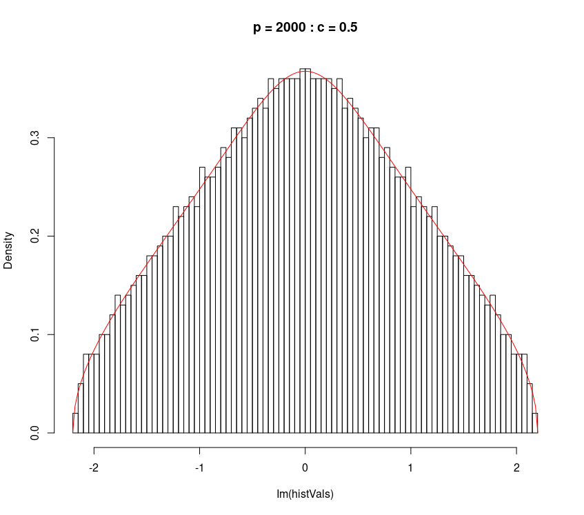
(a) c=0.5

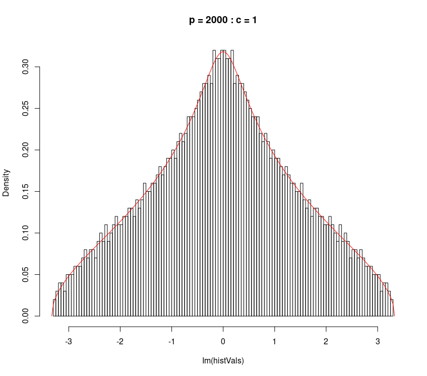
(b) c=1

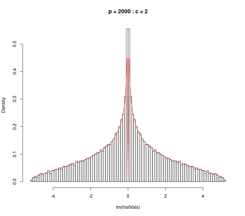
(c) c=2

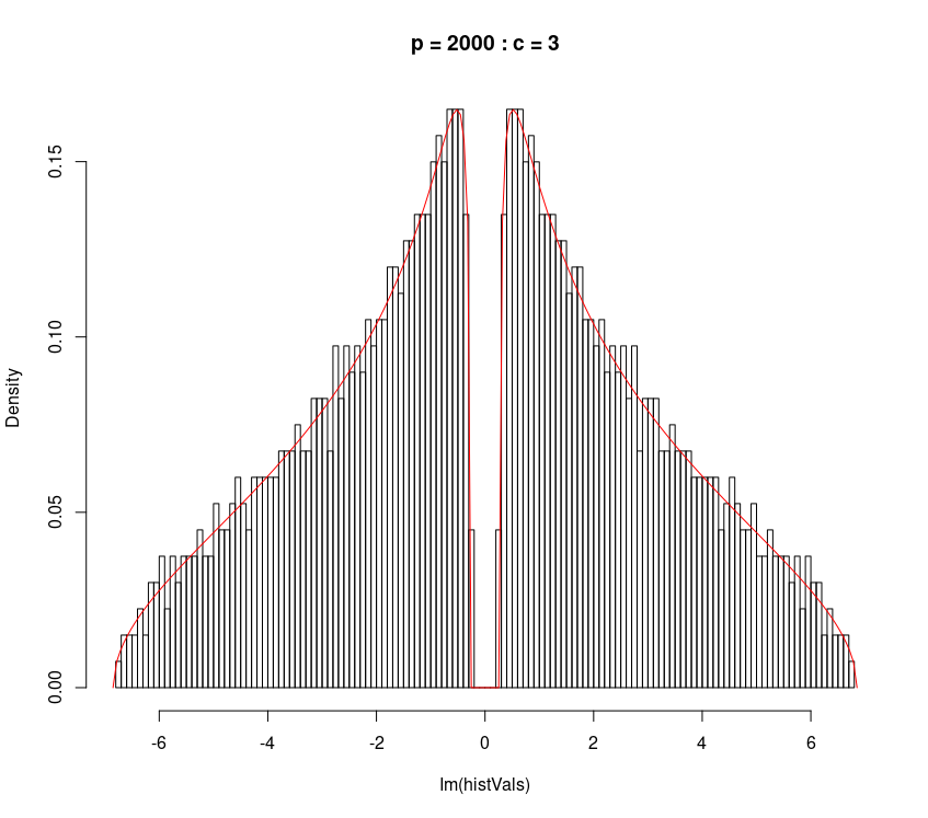
(d) c=3

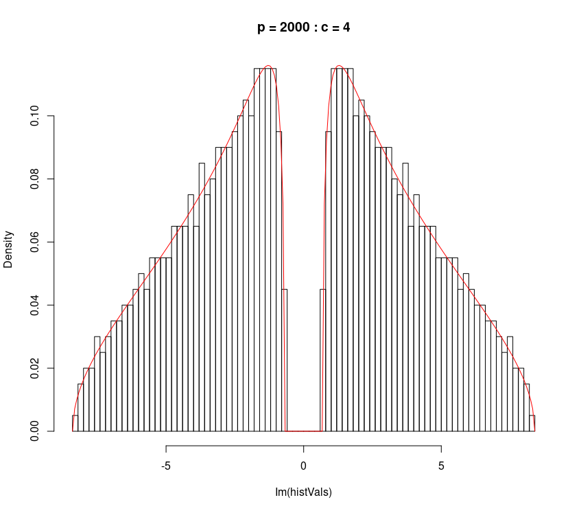
(e) c=4

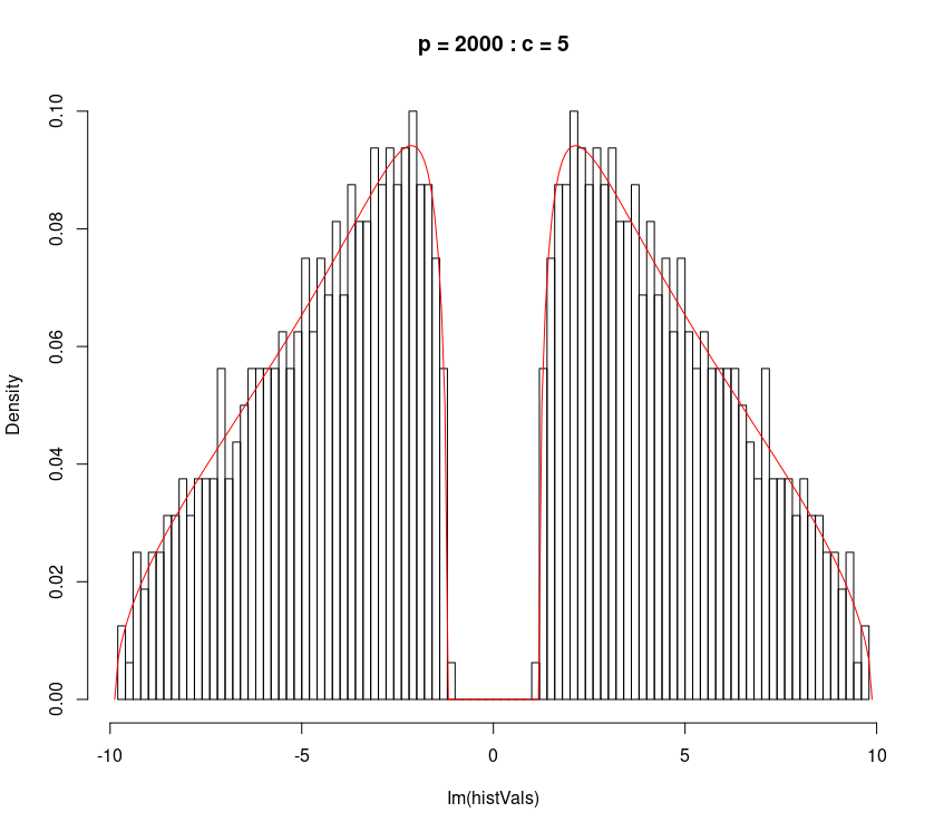
(f) c=5

Figure 1. Simulated vs. theoretical limit distributions at various levels of $c$ for $\Sigma_{n}=I_{p}$

6. The Hermitian Case

We have also derived analogous results case for the Hermitian case (i.e. $S_{n}^{+}$ in (1.1)). The conditions under which the ESDs of $S_{n}^{+}$ approach a non-random limit are exactly the same as those in Theorem 4.1. The main result is stated below.

Theorem 6.1.

Let $S_{n}^{+}$ be as defined in (1.1). Under (T1-T4) of Theorem 4.1, $F^{S_{n}^{+}}\xrightarrow{d}F^{+}$ a.s. where $F^{+}$ is a non-random distribution with Stieltjes Transform at $z\in\mathbb{C}^{+}$ given by

(6.1) $$s(z)=\dfrac{1}{z}\bigg{(}\dfrac{2}{c}-1\bigg{)}+\dfrac{1}{cz}\bigg{(}\dfrac{1}{-1+ch(z)}-\dfrac{1}{1+ch(z)}\bigg{)}$$

where $h(z)\in\mathbb{C}^{+}$ is the unique number such that

(6.2) $$h(z)=\int\dfrac{\lambda dH(\lambda)}{\bigg{[}-z+\lambda\bigg{(}\dfrac{1}{1+ch(z)}+\dfrac{1}{-1+ch(z)}\bigg{)}\bigg{]}}$$

Further $h$ is analytic in $\mathbb{C}^{+}$ and has a continuous dependence on $H$.

The proof can be found in Appendix D.

Similar results as those in Section 5 have also been established for the Hermitian case. As mentioned in the introduction, the limiting distribution (support, point mass at $0$, density) is exactly the same as the one in the skew-Hermitian case except that it is supported on the real axis.

Acknowledgement

The authors are grateful to Professor Arup Bose for some insightful discussions and suggestions.

Appendix A General Results

A.1. A few basic results related to matrices

• (R0): Resolvent identity: $A^{-1}-B^{-1}=A^{-1}(B-A)B^{-1}=B^{-1}(B-A)A^{-1}$

• (R1) For $p\times p$ skew-Hermitian matrices A and B, $||F^{A}-F^{B}||_{im}=||F^{-\mathbbm{i}A}-F^{-\mathbbm{i}B}||\leq\frac{1}{p}\operatorname{rank}(A-B)$

  The first equality follows from (3.5) and the last inequality follows from Lemma 2.4 of [15].

• (R2) For a rectangular matrix, we have $\operatorname{rank}(A)\leq$ the number of non-zero entries of A. This is a result from Lemma 2.1 of [15].

• (R3) $\operatorname{rank}(AXB-PXQ)\leq\operatorname{rank}(A-P)+\operatorname{rank}(B-Q)$ where the dimensions of relevant matrices are compatible

• (R4) Cauchy Schwarz Inequality: $|a^{*}Xb|\leq||X||_{op}|a|_{2}|b|_{2}$ where $|a|_{2}=\sqrt{a^{*}a}$

• (R5) For a p.d. matrix B and any square matrix A, $|\operatorname{trace}(AB)|\leq||A||_{op}\operatorname{trace}(B)$.

  To see this let $B=LL^{*}$ and let $L=[L_{1}:\ldots:L_{n}]$ and $B=(B_{ij})_{ij}$. Using (R4) of A.1 we get,

  $$|\operatorname{trace}(AB)|=|\operatorname{trace}(ALL^{*})|=|\operatorname{trace}(L^{*}AL)|=|\sum_{j=1}^{n}L_{j}^{*}AL_{j}|\leq\sum_{j=1}^{n}|L_{j}^{*}AL_{j}|$$

  $$\leq \sum_{j=1}^{n}||A||_{op}L_{j}^{*}L_{j}=\sum_{j=1}^{n}||A||_{op}B_{jj}=||A||_{op}\operatorname{trace}(B)$$

• ((R6)) For $A,B\in\mathbb{R}^{N\times N}$, $|\operatorname{trace}(AB)|\leq N||A||_{op}||B||_{op}$

Lemma A.1.

Let $\{F_{n},G_{n}\}_{n=1}^{\infty}$ be sequences of distribution functions on $\mathbbm{i}\mathbb{R}$ with $s_{F_{n}}(z),s_{G_{n}}(z)$ denoting their respective Stieltjes transforms at $z\in\mathbb{C}_{L}$. If $L_{im}(F_{n},G_{n})\rightarrow 0$, then $|s_{F_{n}}(z)-s_{G_{n}}(z)|\rightarrow 0$.

Proof.

For a distribution function $F$ on $\mathbbm{i}\mathbb{R}$, we denote its real counterpart as $\tilde{F}$. Let $\mathcal{P}(\mathbb{R})$ represent the set of all probability distribution functions on $\mathbb{R}$. Then the bounded Lipschitz metric is defined as follows

$$\beta:\mathcal{P}(\mathbb{R})\times\mathcal{P}(\mathbb{R})\rightarrow\mathbb{R}_{+}\text{, where }\beta(\tilde{F},\tilde{G}):=\underset{}{\sup}\bigg{\{}\bigg{|}\int hd\tilde{F}-\int hd\tilde{G}\bigg{|}:||h||_{BL}\leq 1\bigg{\}}$$

$$\text{and }||h||_{BL}=\sup\{|h(x)|:x\in\mathbb{R}\}+\underset{x\neq y}{\sup}\dfrac{|h(x)-h(y)|}{|x-y|}$$

From Corollary 18.4 and Theorem 8.3 of [8], we have the following relationship between Levy (L) and bounded Lipschitz ($\beta$) metrics.

(A.1) $$\frac{1}{2}\beta(\tilde{F},\tilde{G})\leq L(\tilde{F},\tilde{G})\leq 3\sqrt{\beta(\tilde{F},\tilde{G})}$$

Fix $z\in\mathbb{C}_{L}$ arbitrarily. Define $g_{z}(x):=(\mathbbm{i}x-z)^{-1}$. First of all, $|g_{z}(x)|\leq 1/|\Re(z)|$ $\forall x\in\mathbb{R}$. Also,

$$|g_{z}(x_{1})-g_{z}(x_{2})|=\bigg{|}\frac{1}{\mathbbm{i}x_{1}-z}-\frac{1}{\mathbbm{i}x_{2}-z}\bigg{|}=\frac{|x_{1}-x_{2}|}{|\mathbbm{i}x_{1}-z||\mathbbm{i}x_{2}-z|}\leq|x_{1}-x_{2}|\frac{1}{\Re^{2}(z)}$$

Note that $||g_{z}||_{BL}\leq{1}/{|\Re(z)|}+{1}/{\Re^{2}(z)}<\infty$. Then for $g:={g_{z}}/{||g_{z}||_{BL}}$, we have $||g||_{BL}=1$.

By (A.1) and (3.7), we have

$$L_{im}(F_{n},G_{n})\rightarrow 0\leftrightarrow L(\tilde{F}_{n},\tilde{G}_{n})\rightarrow 0$$

$$\leftrightarrow \beta(\tilde{F}_{n},\tilde{G}_{n})\rightarrow 0$$

$$\implies \bigg{|}\int_{\mathbb{R}}g(x)d\tilde{F}_{n}(x)-\int_{\mathbb{R}}g(x)d\tilde{G}_{n}(x)\bigg{|}\rightarrow 0$$

$$\implies \bigg{|}\int_{\mathbb{R}}\frac{1}{\mathbbm{i}x-z}dF_{n}(x)-\int_{\mathbb{R}}\frac{1}{\mathbbm{i}x-z}dG_{n}(x)\bigg{|}\rightarrow 0$$

$$\implies |s_{F_{n}}(z)-s_{G_{n}}(z)|\longrightarrow 0$$

∎

We state the following result (Lemma B.26 of [2]) without proof.

Lemma A.2.

Let $A=(a_{ij})$ be an $n\times n$ non-random matrix and $x=(x_{1},\ldots,x_{n})^{T}$ be a vector of independent entries. Suppose $\mathbb{E}x_{i}=0,\mathbb{E}|x_{i}|^{2}=1$, and $\mathbb{E}|x_{i}|^{l}\leq\nu_{l}$. Then for $k\geq 1$, $\exists$ $C_{k}>0$ independent of $n$ such that

$$\mathbb{E}|x^{*}Ax-\operatorname{trace}(A)|^{k}\leq C_{k}\bigg{(}(\nu_{4}\operatorname{trace}(AA^{*}))^{\frac{k}{2}}+\nu_{2k}\operatorname{trace}\{(AA^{*})^{\frac{k}{2}}\}\bigg{)}$$

Simplification: For deterministic matrix $A$ with $||A||_{op}<\infty$, let $B=\frac{A}{||A||_{op}}$. Then $||B||_{op}=1$ and by (R6) of A.1, $\operatorname{trace}(BB^{*})\leq n||B||_{op}^{2}=n$ and $\operatorname{trace}\{(BB^{*})^{\frac{k}{2}}\}\leq n||B||_{op}^{k}=n$. Then by Lemma A.2, we have

$$\mathbb{E}|x^{*}Bx-\operatorname{trace}(B)|^{k}\leq C_{k}\bigg{(}(\nu_{4}\operatorname{trace}(BB^{*}))^{\frac{k}{2}}+\nu_{2k}\operatorname{trace}\{(BB^{*})^{\frac{k}{2}}\}\bigg{)}$$

$$\implies \frac{\mathbb{E}|x^{*}Ax-\operatorname{trace}(A)|^{k}}{||A||_{op}^{k}}\leq C_{k}[(n\nu_{4})^{\frac{k}{2}}+n\nu_{2k}]$$

(A.2) $$\implies \mathbb{E}|x^{*}Ax-\operatorname{trace}(A)|^{k}\leq C_{k}||A||_{op}^{k}[(n\nu_{4})^{\frac{k}{2}}+n\nu_{2k}]$$

We will be using this form of the inequality going forward.

Lemma A.3.

Let $\{z_{jn}:1\leq j\leq n\}$ be a triangular array of complex valued random vectors. For $1\leq r\leq n$, denote the $r^{th}$ element of $z_{jn}$ as $z_{jn}^{(r)}$. Suppose $\mathbb{E}z_{jn}^{(r)}=0,\mathbb{E}|z_{jn}^{(r)}|^{2}=1$ and for $k\geq 1$, $\nu_{k}:=\mathbb{E}|z_{jn}^{(r)}|^{k}\leq n^{ak}$ where $0<a<\frac{1}{4}$. Suppose $A$ is independent of $z_{jn}$ and $||A||_{op}\leq B$ a.s. for some $B>0$. Then,

$$\underset{1\leq j\leq n}{\max}\left|\dfrac{1}{n}z_{jn}^{*}Az_{jn}-\dfrac{1}{n}\operatorname{trace}(A)\right|\xrightarrow{a.s}0$$

Proof.

For arbitrary $\epsilon>0$ and $k\geq 1$, we have

$$p_{n}:= \mathbb{P}\bigg{(}\underset{1\leq j\leq n}{\max}\left|\dfrac{1}{n}z_{jn}^{*}Az_{jn}-\dfrac{1}{n}\operatorname{trace}(A)\right|>\epsilon\bigg{)}$$

$$\leq \sum_{j=1}^{n}\mathbb{P}\bigg{(}\left|\dfrac{1}{n}z_{jn}^{*}Az_{jn}-\dfrac{1}{n}\operatorname{trace}(A)\right|>\epsilon\bigg{)}\text{, by union bound}$$

$$\leq \sum_{j=1}^{n}\dfrac{\mathbb{E}\left|\dfrac{1}{n}z_{jn}^{*}Az_{jn}-\dfrac{1}{n}\operatorname{trace}(A)\right|^{k}}{\epsilon^{k}}\text{, for any }k\in\mathbb{N}$$

$$= \sum_{j=1}^{n}\dfrac{\mathbb{E}\bigg{(}\mathbb{E}\bigg{[}|\dfrac{1}{n}z_{jn}^{*}Az_{jn}-\dfrac{1}{n}\operatorname{trace}(A)|^{k}\bigg{|}A\bigg{]}\bigg{)}}{\epsilon^{k}}$$

$$\leq \sum_{j=1}^{n}\dfrac{\mathbb{E}||A||_{op}^{k}C_{k}((n\nu_{4})^{\frac{k}{2}}+n\nu_{2k})}{n^{k}\epsilon^{k}}\text{ by }(\ref{I1})$$

$$\leq \sum_{j=1}^{n}\dfrac{K[(n^{1+4a})^{\frac{k}{2}}+n^{1+2ak}]}{n^{k}}\text{, where }K=C_{k}\bigg{(}\frac{B}{\epsilon}\bigg{)}^{k}$$

$$= \dfrac{nK[n^{\frac{k}{2}+2ak}+n^{1+2ak}]}{n^{k}}=\frac{K}{n^{k(\frac{1}{2}-2a)-1}}+\frac{K}{n^{k(1-2a)-2}}$$

Since $0<a<\frac{1}{4}$, we can choose $k\in\mathbb{N}$ large enough so that $\min\{k(\frac{1}{2}-2a)-1,k(1-2a)-2\}>1$ to ensure that $\sum_{n=1}^{\infty}p_{n}$ converges. Therefore by Borel Cantelli lemma we have the result. ∎

Lemma A.4.

Let $\{X_{jn},Y_{jn}:1\leq j\leq n\}_{n=1}^{\infty}$ be triangular arrays of random variables. Suppose $\underset{1\leq j\leq n}{\max}|X_{jn}|\xrightarrow{a.s.}0$ and $\underset{1\leq j\leq n}{\max}|Y_{jn}|\xrightarrow{a.s.}0$. Then $\underset{1\leq j\leq n}{\max}|X_{jn}+Y_{jn}|\xrightarrow{a.s.}0$.

Proof.

Let $A_{x}:=\{\omega:\underset{n\rightarrow\infty}{\lim}\underset{1\leq j\leq n}{\max}|X_{jn}(\omega)|=0\}$, $A_{y}:=\{\omega:\underset{n\rightarrow\infty}{\lim}\underset{1\leq j\leq n}{\max}|Y_{jn}(\omega)|=0\}$. Then $\mathbb{P}(A_{x})=1=\mathbb{P}(A_{y})$. Then $\forall\omega\in A_{x}\cap A_{y}$, we have $0\leq|X_{jn}(\omega)+Y_{jn}(\omega)|\leq|X_{jn}(\omega)|+|Y_{jn}(\omega)|$. Hence, $\underset{n\rightarrow\infty}{\lim}\underset{1\leq j\leq n}{\max}|X_{jn}(\omega)+Y_{jn}(\omega)|=0$. But, $\mathbb{P}(A_{x}\cap A_{y})=1$. Therefore, the result follows. ∎

Lemma A.5.

Let $\{A_{jn},B_{jn},C_{jn},D_{jn}:1\leq j\leq n\}_{n=1}^{\infty}$ be triangular arrays of random variables. Suppose $\underset{1\leq j\leq n}{\max}|A_{jn}-C_{jn}|\xrightarrow{a.s.}0$ and $\underset{1\leq j\leq n}{\max}|B_{jn}-D_{jn}|\xrightarrow{a.s.}0$ and $\exists N_{0}\in\mathbb{N}$ such that $|C_{jn}|\leq B_{1}$ a.s. and $|D_{jn}|\leq B_{2}$ a.s. when $n>N_{0}$ for some $B_{1},B_{2}\geq 0$. Then $\underset{1\leq j\leq n}{\max}|A_{jn}B_{jn}-C_{jn}D_{jn}|\xrightarrow{a.s.}0$.

Proof.

Let $\Omega_{1}=\{\omega:\underset{n\rightarrow\infty}{\lim}\underset{1\leq j\leq n}{\max}|A_{jn}(\omega)-C_{jn}(\omega)|=0\}$, $\Omega_{2}=\{\omega:\underset{n\rightarrow\infty}{\lim}\underset{1\leq j\leq n}{\max}|B_{jn}(\omega)-D_{jn}(\omega)|=0\}$, $\Omega_{3}=\{\omega:|C_{jn}(\omega)|\leq B_{1}\text{ for }n>N_{0}\}$ and $\Omega_{4}=\{\omega:|D_{jn}(\omega)|\leq B_{2}\text{ for }n>N_{0}\}$. Then $\Omega_{0}=\cap_{j=1}^{4}\Omega_{j}$ is a set of probability $1$. Then $\forall\omega\in\Omega_{0}$, $\underset{1\leq j\leq n}{\max}|B_{jn}(\omega)|\leq B_{2}$ eventually for large $n$. Therefore for $\omega\in\Omega_{0}$ and large $n$,

$$\underset{1\leq j\leq n}{\max}|A_{jn}B_{jn}-C_{jn}D_{jn}|\leq \underset{1\leq j\leq n}{\max}|A_{jn}-C_{jn}||B_{jn}|+\underset{1\leq j\leq n}{\max}|C_{jn}||B_{jn}-D_{jn}|$$

$$\leq B_{2}\underset{1\leq j\leq n}{\max}|A_{jn}-C_{jn}|+B_{1}\underset{1\leq j\leq n}{\max}|B_{jn}-D_{jn}|\xrightarrow{a.s.}0$$

∎

Lemma A.6.

Let $\{X_{jn},Y_{jn}:1\leq j\leq n\}_{n=1}^{\infty}$ be triangular arrays of random variables such that $\underset{1\leq j\leq n}{\max}|X_{jn}-Y_{jn}|\xrightarrow{a.s.}0$. Then $|\frac{1}{n}\sum_{j=1}^{n}(X_{jn}-Y_{jn})|\xrightarrow{a.s.}0$.

Proof.

Let $M_{n}:=\underset{1\leq j\leq n}{\max}|X_{jn}-Y_{jn}|$. We have $|\frac{1}{n}\sum_{j=1}^{n}(X_{jn}-Y_{jn})|\leq\frac{1}{n}\sum_{j=1}^{n}|X_{jn}-Y_{jn}|\leq M_{n}$. Let $\epsilon>0$ be arbitrary. Then $\exists\Omega_{0}\subset\Omega$ such that $\mathbb{P}(\Omega_{0})=1$ and $\forall\omega\in\Omega_{0}$, we have $M_{n}(\omega)<\epsilon$ for sufficiently large $n\in\mathbb{N}$. Then, $\mathbb{P}(\{\omega:|\frac{1}{n}\sum_{j=1}^{n}(X_{jn}-Y_{jn})|<\epsilon\})=1$. Since $\epsilon>0$ is arbitrary, the result follows. ∎

Lemma A.7.

Let $B\in\mathbb{C}^{p\times p}$ be of the form $B=A-zI_{p}$ for some skew-Hermitian matrix $A$ and $z\in\mathbb{C}_{L}$. For vectors $u,v\in\mathbb{C}^{p}$, define $\langle u,v\rangle:=u^{*}B^{-1}v$. Then,

1:

$(B+uv^{*}-vu^{*})^{-1}u=B^{-1}(\alpha_{1}u+\beta_{1}v)$; $\alpha_{1}=(1-\langle u,v\rangle)D(u,v)$; $\beta_{1}=\langle u,u\rangle D(u,v)$

2:

$(B+uv^{*}-vu^{*})^{-1}v=B^{-1}(\alpha_{2}v+\beta_{2}u)$; $\alpha_{2}=(1+\langle v,u\rangle)D(u,v)$; $\beta_{2}=-\langle v,v\rangle D(u,v)$

where $D(u,v)=\bigg{(}(1-\langle u,v\rangle)(1+\langle v,u\rangle)+\langle u,u\rangle\langle v,v\rangle\bigg{)}^{-1}$

Proof.

Clearly, $B$ cannot have zero as eigenvalue. So $\langle u,v\rangle$ is well defined. For $P\in\mathbb{C}^{p\times p},Q,R\in\mathbb{C}^{p\times n}$ with $P+QR^{*}$ and $P$ being invertible, the Woodbury formula states that

(A.4) $$(P+QR^{*})^{-1}= P^{-1}-P^{-1}Q(I_{n}+R^{*}P^{-1}Q)^{-1}R^{*}P^{-1}$$

$$\implies(P+QR^{*})^{-1}Q= P^{-1}Q-P^{-1}Q(I_{n}+R^{*}P^{-1}Q)^{-1}R^{*}P^{-1}Q$$

$$= P^{-1}Q\bigg{(}I_{n}-(I_{n}+R^{*}P^{-1}Q)^{-1}R^{*}P^{-1}Q\bigg{)}$$

Let $P=B$, $Q=[u:v]$ and $R=[v:-u]$. Note that $\operatorname{det}(I_{2}+R^{*}P^{-1}Q)^{-1}=D(u,v)$. So, $D(u,v)$ is well-defined. Finally, observing that $B+uv^{*}-vu^{*}=P+QR^{*}$, we use (A.4) to get

$$(B+uv^{*}-vu^{*})^{-1}[u:v]$$

$$= B^{-1}[u:v]\bigg{(}I_{2}-(I_{2}+R^{*}P^{-1}Q)^{-1}R^{*}P^{-1}Q\bigg{)}$$

$$= B^{-1}[u:v]\bigg{(}I_{2}-{\begin{bmatrix}1+\langle v,u\rangle&\langle v,v\rangle\\ -\langle u,u\rangle&1-\langle u,v\rangle\end{bmatrix}}^{-1}\begin{bmatrix}\langle v,u\rangle&\langle v,v\rangle\\ -\langle u,u\rangle&-\langle u,v\rangle\\ \end{bmatrix}\bigg{)}$$

$$= B^{-1}[u:v]\bigg{(}I_{2}-D(u,v)\begin{bmatrix}1-\langle u,v\rangle&-\langle v,v\rangle\\ \langle u,u\rangle&1+\langle v,u\rangle\end{bmatrix}\begin{bmatrix}\langle v,u\rangle&\langle v,v\rangle\\ -\langle u,u\rangle&-\langle u,v\rangle\\ \end{bmatrix}\bigg{)}$$

$$= D(u,v)B^{-1}[u:v]\begin{bmatrix}\alpha_{1}&\beta_{2}\\ \beta_{1}&\alpha_{2}\end{bmatrix}$$

∎

Appendix B Proofs related to Section 4

B.1. A few preliminary results

Here we establish a few results that are required to prove the main theorems of Section 4. All of them (except Lemma B.1) are proved under Assumptions 4.3.1. These results directly lead to the proofs of Theorem 4.7 and Theorem 4.9.

Lemma B.1.

Under the conditions of Theorem 4.1, if we instead had $H=\delta_{0}$, we have $F^{S_{n}}\xrightarrow{d}\delta_{0}$ a.s. When $H\neq\delta_{0}$, $\{F^{S_{n}}\}_{n=1}^{\infty}$ is a tight sequence.

Proof.

Let $A:=\frac{1}{\sqrt{n}}[Z1:Z2]$ and $B:=\frac{1}{\sqrt{n}}[Z_{2}:-Z_{1}]^{*}$. Then, $S_{n}=\Sigma_{n}^{\frac{1}{2}}AB\Sigma_{n}^{\frac{1}{2}}$. Now define $M_{n}=AB\Sigma_{n}$. Note that $S_{n}$ and $M_{n}$ share the same set of eigenvalues and

$$Z_{0n}:=\frac{1}{n}(Z_{1}Z_{1}^{*}+Z_{2}Z_{2}^{*})=AA^{*}=B^{*}B$$

In the equations to follow, we highlight the fact that the support of $F^{S_{n}}$ (and hence of $F^{M_{n}}$) is purely imaginary. However, the supports of $F^{\sqrt{M_{n}M_{n}^{*}}}$, $F^{Z_{0n}}$ and $F^{\Sigma_{n}}$ are purely real.

For arbitrary $K_{1},K_{2},K_{3}>0$, let $K=K_{1}K_{2}K_{3}$. Using Lemma 2.3 of [15],

$$F^{S_{n}}\{(-\infty,-\mathbbm{i}K)\cup(\mathbbm{i}K,\infty)\}= F^{M_{n}}\{(-\infty,-\mathbbm{i}K)\cup(\mathbbm{i}K,\infty)\}$$

$$= F^{\sqrt{M_{n}M_{n}^{*}}}\{(K,\infty)\}$$

$$\leq F^{\sqrt{AA^{*}}}\{(K_{1},\infty)\}+F^{\sqrt{BB^{*}}}\{(K_{2},\infty)\}+F^{\sqrt{\Sigma_{n}^{2}}}\{(K_{3},\infty)\}$$

(B.1) $$= F^{Z_{0n}}\{(K_{1}^{2},\infty)\}+F^{Z_{0n}}\{(K_{2}^{2},\infty)\}+F^{{\Sigma_{n}}}\{(K_{3},\infty)\}$$

In the second term of the last equality, we used the fact that $BB^{*}$ and $B^{*}B$ share the same set of eigenvalues.

Now we prove the first result. Suppose $F^{\Sigma_{n}}\xrightarrow{d}H=\delta_{0}$ a.s. Choose $\epsilon,K_{1},K_{2}>0$ arbitrarily and set $K_{3}={\epsilon}/{K_{1}K_{2}}$. Since $\{F^{\Sigma}_{n}\}_{n=1}^{\infty}$ converges weakly to $\delta_{0}$,

$$\underset{n\rightarrow\infty}{\limsup}F^{{\Sigma_{n}}}\bigg{\{}(\dfrac{\epsilon}{K_{1}K_{2}},\infty)\bigg{\}}=0$$

Note that $\{F^{Z_{0n}}\}_{n=1}^{\infty}$ is a tight sequence. Now letting $K_{1},K_{2}\rightarrow\infty$ in (B.1), we see that

$$\underset{n\rightarrow\infty}{\limsup}F^{S_{n}}\{(-\infty,-\epsilon)\cup(\epsilon,\infty)\}\leq\underset{K_{1}\rightarrow\infty}{\lim}F^{Z_{0n}}\{(K_{1}^{2},\infty)\}+\underset{K_{2}\rightarrow\infty}{\lim}F^{Z_{0n}}\{(K_{2}^{2},\infty)\}=0$$

Since $\epsilon>0$ was chosen arbitrarily, we conclude that $F^{S_{n}}\xrightarrow{d}\delta_{0}$ a.s. This justifies why we exclusively stick to the case where $H\neq\delta_{0}$ in Theorem 4.1.

Now suppose$F^{\Sigma_{n}}\xrightarrow{d}H\neq\delta_{0}$ a.s. The tightness of $\{F^{S_{n}}\}_{n=1}^{\infty}$ is immediate from (B.1) upon observing the tightness of $\{F^{Z_{0n}}\}_{n=1}^{\infty}$ and $\{F^{\Sigma_{n}}\}_{n=1}^{\infty}$. ∎

Lemma B.2.

Let $M_{n}\in\mathbb{C}^{p\times p}$ be a sequence of deterministic matrices with bounded operator norm, i.e. $||M_{n}||_{op}\leq B$ for some $B\geq 0$. Under Assumptions 4.3.1, for $z\in\mathbb{C}_{L}$ and sufficiently large $n$, we have

$$\underset{1\leq j\leq n}{\max}|\operatorname{trace}\{M_{n}Q(z)\}-\operatorname{trace}\{M_{n}Q_{-j}(z)\}|\leq\dfrac{4cCB}{\Re^{2}(z)}\text{ a.s.}$$

Consequently, $\underset{1\leq j\leq n}{\max}|\frac{1}{p}\operatorname{trace}\{M_{n}(Q-Q_{-j})\}|\xrightarrow{a.s.}0$

Proof.

By (R0) and (R4) of (A.1), for any $1\leq j\leq n$,

$$|\operatorname{trace}\{M_{n}Q\}-\operatorname{trace}\{M_{n}Q_{-j}\}|$$

$$= |\operatorname{trace}\{M_{n}(S_{n}-zI_{p})^{-1}\}-\operatorname{trace}\{M_{n}(S_{nj}-zI_{p})^{-1}\}|$$

$$= |\operatorname{trace}\{M_{n}Q(\dfrac{1}{n}X_{1j}X_{2j}^{*}-\dfrac{1}{n}X_{2j}X_{1j}^{*})Q_{-j}\}|$$

$$= \frac{1}{n}|X_{2j}^{*}Q_{-j}M_{n}QX_{1j}-X_{1j}^{*}Q_{-j}M_{n}QX_{2j}|$$

$$\leq \dfrac{1}{n}|X_{2j}^{*}Q_{-j}MQX_{1j}|+\dfrac{1}{n}|X_{1j}^{*}Q_{-j}MQX_{2j}|$$

(B.2) $$\leq ||Q_{-j}M_{n}Q||_{op}\bigg{(}\sqrt{\frac{1}{n}X_{2j}^{*}X_{2j}}\sqrt{\frac{1}{n}X_{1j}^{*}X_{1j}}+\sqrt{\frac{1}{n}X_{1j}^{*}X_{1j}}\sqrt{\frac{1}{n}X_{2j}^{*}X_{2j}}\bigg{)}$$

First of all, we have

$$||Q_{-j}M_{n}Q||_{op}<B/\Re^{2}(z)\text{ since }||Q_{-j}||_{op},||Q||_{op}\leq 1/|\Re(z)|,||M_{n}||_{op}<B$$

Secondly, for $k\in\{1,2\}$, we have $X_{kj}^{*}X_{kj}=Z_{kj}^{*}\Sigma_{n}Z_{kj}$ where $\Sigma_{n}$ satisfies A1 and $Z_{1},Z_{2}$ satisfy A2 respectively of Assumptions 4.3.1. Let $z_{jn}=Z_{kj},1\leq j\leq n,n\in\mathbb{N}$ and $A=\Sigma_{n}$. Then by Lemma A.3, we have

$$\underset{1\leq j\leq n}{\max}\bigg{|}\frac{1}{n}X_{kj}^{*}X_{kj}-\frac{1}{n}\operatorname{trace}(\Sigma_{n})\bigg{|}\xrightarrow{a.s.}0.$$

From (T1) and (T4) of Theorem 4.1,

$$\dfrac{1}{n}\operatorname{trace}(\Sigma_{n})=c_{n}\bigg{(}\dfrac{1}{p}\operatorname{trace}(\Sigma_{n})\bigg{)}<2cC$$

for sufficiently large $n$. This implies that for $k\in\{1,2\}$ and large $n$,

$$\underset{1\leq j\leq n}{\max}\bigg{|}\frac{1}{n}X_{kj}^{*}X_{kj}\bigg{|}<2cC\text{ a.s.}$$

Combining everything with (B.2), for large $n$, we must have

$$\underset{1\leq j\leq n}{\max}|\operatorname{trace}\{M_{n}Q\}-\operatorname{trace}\{M_{n}Q_{-j}\}|\leq\frac{B}{\Re^{2}(z)}(2cC+2cC)=\frac{4cCB}{\Re^{2}(z)}\text{ a.s.}$$

For $z\in\mathbb{C}_{L}$, it is clear that for arbitrary $\epsilon>0$, $\underset{1\leq j\leq n}{\max}|\frac{1}{p}\operatorname{trace}\{M(Q-Q_{-j})\}|<\epsilon$ a.s. for large $n$. Therefore, $\underset{1\leq j\leq n}{\max}|\frac{1}{p}\operatorname{trace}\{M(Q-Q_{-j})\}|\xrightarrow{a.s.}0$.

∎

Lemma B.3.

Concentration of Stieltjes Transforms Under Assumptions 4.3.1 for $z\in\mathbb{C}_{L}$, we have $|s_{n}(z)-\mathbb{E}s_{n}(z)|\xrightarrow{a.s.}0$ and $|h_{n}(z)-\mathbb{E}h_{n}(z)|\xrightarrow{a.s.}0$ .

Proof.

Define $\mathcal{F}_{k}=\sigma(\{X_{1j},X_{2j}:k+1\leq j\leq n\})$ and for a measurable function $f$, we denote $\mathbb{E}_{k}f(X):=\mathbb{E}(f(X)|\mathcal{F}_{k})$ for $0\leq k\leq n-1$ and $\mathbb{E}_{n}f(X):=\mathbb{E}f(X)$. Then, we observe that

$$h_{n}(z)-\mathbb{E}h_{n}(z)= \dfrac{1}{p}\operatorname{trace}\{\Sigma_{n}Q\}-\mathbb{E}\bigg{(}\dfrac{1}{p}\operatorname{trace}\{\Sigma_{n}Q\}\bigg{)}$$

$$= \dfrac{1}{p}\sum_{k=1}^{n}(\mathbb{E}_{k}-\mathbb{E}_{k-1})\operatorname{trace}\{\Sigma_{n}Q\}$$

$$= \dfrac{1}{p}\sum_{k=1}^{n}(\mathbb{E}_{k}-\mathbb{E}_{k-1})\underbrace{(\operatorname{trace}\{\Sigma_{n}Q\}-\operatorname{trace}\{\Sigma_{n}Q_{-k}\})}_{:=Y_{k}}$$

$$= \dfrac{1}{p}\sum_{k=1}^{n}\underbrace{(\mathbb{E}_{k}-\mathbb{E}_{k-1})Y_{k}}_{:=D_{k}}=\frac{1}{p}\sum_{k=1}^{n}D_{k}$$

From (B.2), we have

$$|Y_{k}|=|\operatorname{trace}\{\Sigma_{n}Q\}-\operatorname{trace}\{\Sigma_{n}Q_{j}\}|\leq\dfrac{\tau}{\Re^{2}(z)}W_{nk}\text{, where }W_{nk}:=\frac{1}{n}(||X_{1k}||^{2}+||X_{2k}||^{2})$$

So, we have $\left|D_{k}\right|\leq\dfrac{2\tau}{\Re^{2}(z)}W_{nk}$. By Lemma 2.12 of [2], there exists $K_{4}$ depending only on $z\in\mathbb{C}_{L}$ such that

(B.3) $$\mathbb{E}\left|h_{n}(z)-\mathbb{E}h_{n}(z)\right|^{4}=\mathbb{E}\left|\frac{1}{p}\sum_{k=1}^{n}D_{k}\right|^{4}\leq \frac{K_{4}}{p^{4}}\mathbb{E}\bigg{(}\sum_{k=1}^{n}|D_{k}|^{2}\bigg{)}^{2}\leq\frac{16K_{4}\tau^{4}}{p^{4}\Re^{8}(z)}\mathbb{E}\bigg{(}\sum_{k=1}^{n}|W_{nk}|^{2}\bigg{)}^{2}$$

$$= \frac{K_{0}}{p^{4}}\mathbb{E}\bigg{(}\sum_{k=1}^{n}|W_{nk}|^{4}+\sum_{k\neq l}|W_{nk}|^{2}|W_{nl}|^{2}\bigg{)}$$

$$= \frac{K_{0}}{p^{4}}\bigg{(}\sum_{k=1}^{n}\mathbb{E}|W_{nk}|^{4}+\sum_{k\neq l}\mathbb{E}|W_{nk}|^{2}\mathbb{E}|W_{nl}|^{2}\bigg{)}$$

We have the following inequalities.

1. $||X_{1k}||^{m}=(Z_{1k}^{*}\Sigma_{n}Z_{1k})^{\frac{m}{2}}\leq(||\Sigma_{n}||_{op}||Z_{1k}||^{2})^{\frac{m}{2}}\leq\tau^{\frac{r}{2}}||Z_{1k}||^{m}$ for $m\geq 1$

2. $|W_{nk}|^{2}\leq\dfrac{2}{n^{2}}(||X_{1k}||^{4}+||X_{2k}||^{4})\leq\dfrac{2\tau^{2}}{n^{2}}(||Z_{1k}||^{4}+||Z_{2k}||^{4})$

3. $|W_{nk}|^{4}\leq\dfrac{8}{n^{4}}(||X_{1k}||^{8}+||X_{2k}||^{8})\leq\dfrac{8\tau^{4}}{n^{4}}(||Z_{1k}||^{8}+||Z_{2k}||^{8})$

Recall that $Z_{1k}$ is the $k^{th}$ column of $Z_{1}$ and $z_{jk}^{(1)}$ represents the $j^{th}$ element of $Z_{1k}$. Let $M_{4}>0$ be such that for $r=1,2$, $\mathbb{E}|z_{ij}^{(r)}|^{4}\leq M_{4}$. This exists since the entries of $Z_{1},Z_{2}$ have uniform bound on moments of order $4+\eta_{0}$. So, we have

$$\mathbb{E}||Z_{1k}||^{4}=\mathbb{E}\bigg{(}\sum_{j=1}^{p}|z_{jk}^{(1)}|^{2}\bigg{)}^{2}=\mathbb{E}\bigg{(}\sum_{j=1}^{p}|z_{jk}^{(1)}|^{4}+\sum_{j\neq l}|z_{jk}^{(1)}|^{2}|z_{lk}^{(1)}|^{2}\bigg{)}\leq pM_{4}+p(p-1)$$

and, by Assumptions 4.3.1, $\mathbb{E}|z_{jk}^{(1)}|^{m}\leq n^{ma}$, for $m\geq 1$, with $0<a<1/4$,

$$\mathbb{E}||Z_{1k}||^{8}=\mathbb{E}\bigg{(}\sum_{j=1}^{p}|z_{jk}^{(1)}|^{2}\bigg{)}^{4}= \mathbb{E}\bigg{(}\sum_{j=1}^{p}|z_{jk}^{(1)}|^{8}+\sum_{j\neq l}|z_{jk}^{(1)}|^{6}|z_{lk}^{(1)}|^{2}+\sum_{j\neq l}|z_{jk}^{(1)}|^{4}|z_{lk}^{(1)}|^{4}\bigg{)}$$

$$\leq p\times(M_{4}n^{12a})^{1/2}+p(p-1)\times(M_{4}n^{8a})^{1/2}\times 1+p(p-1)\times M_{4}^{2}$$

$$\leq p(M_{4}n^{12a})^{1/2}+p^{2}(M_{4}n^{8a})^{1/2}+p^{2}M_{4}^{2}$$

where the bounds in the second last line follows from $\mathbb{E}|z_{jk}^{(1)}|^{8}\leq(\mathbb{E}|z_{jk}^{(1)}|^{4}\mathbb{E}|z_{jk}^{(1)}|^{12})^{1/2}$, and $\mathbb{E}|z_{jk}^{(1)}|^{6}\leq(\mathbb{E}|z_{jk}^{(1)}|^{4}\mathbb{E}|z_{jk}^{(1)}|^{8})^{1/2}$, by Cauchy-Schwarz inequality. Therefore, combining everything, we get

$$\mathbb{E}|W_{nk}|^{2}\leq \frac{4\tau^{2}}{n^{2}}\bigg{(}pM_{4}+p(p-1)\bigg{)}\leq 4\tau^{2}c_{n}^{2}(M_{4}/p+1)\text{, recall }c_{n}=p/n$$

$$\mathbb{E}|W_{nk}|^{4}\leq \frac{16\tau^{4}}{n^{4}}\bigg{(}c_{n}M_{4}^{1/2}n^{1+6a}+c_{n}^{2}M_{4}^{1/2}n^{2+4a}+p^{2}M_{4}^{2}\bigg{)}=O\bigg{(}\max\{\frac{1}{n^{3-6a}},\frac{1}{n^{2-4a}}\}\bigg{)}$$

Since $0<a<1/4$, we have $\min\{2-4a,3-6a\}=2-4a>1$. Using these in (B.3) and by Borel Cantelli Lemma, we have $|h_{n}(z)-\mathbb{E}h_{n}(z)|\xrightarrow{a.s.}0$. The other result follows similarly. ∎

Lemma B.4.

Recall definitions of $h_{n}(z)$ (4.3) and $v_{n}(z)$ (B.18). Under A1 of Assumptions 4.3.1, for $z\in\mathbb{C}_{L}$ and sufficiently large $n$, $\Re(c_{n}h_{n}(z))\geq K_{0}$ a.s., $\Re(c_{n}\mathbb{E}h_{n}(z))\geq K_{0}$ and $|v_{n}(z)|\leq 1/K_{0}$ a.s. where $K_{0}>0$ depends on $z,c,\tau$ and $H$.

Proof.

We have $||\Sigma_{n}||_{op}\leq\tau$. Since $F^{\Sigma_{n}}$ and $H$ have a compact support $[0,\tau]$ and $F^{\Sigma_{n}}\xrightarrow{d}H$ a.s., we get $\int_{0}^{\tau}\lambda dF^{\Sigma_{n}}(\lambda)\xrightarrow{}\int_{0}^{\tau}\lambda dH(\lambda)>0$ since $H\neq\delta_{0}$. Therefore,

(B.4) $$\frac{1}{n}\operatorname{trace}(\Sigma_{n})=c_{n}\int_{0}^{\tau}\lambda dF^{\Sigma_{n}}(\lambda)\xrightarrow{}c\int_{0}^{\tau}\lambda dH(\lambda)>0$$

Let $z=-u+\mathbbm{i}v$ with $u>0$. Let $a_{ij}$ represent the $ij^{th}$ element of $A:=P^{*}\Sigma_{n}P$ where $S_{n}=P\Lambda P^{*}$ with $\Lambda=\operatorname{diag}(\{\mathbbm{i}\lambda_{j}\}_{j=1}^{p})$ being a diagonal matrix containing the purely imaginary eigenvalues of $S_{n}$. Then,

$$c_{n}h_{n}=\frac{1}{n}\operatorname{trace}\{\Sigma_{n}Q\}=\frac{1}{n}\operatorname{trace}\{P^{*}\Sigma_{n}P(\Lambda-zI_{p})^{-1}\}=\frac{1}{n}\sum_{j=1}^{p}\frac{a_{jj}}{\mathbbm{i}\lambda_{j}-z}$$

For any $\delta>0$, we have

$$||S_{n}||_{op}=||\frac{1}{n}X_{1}X_{2}^{*}-\frac{1}{n}X_{2}X_{1}^{*}||_{op}\leq 2\sqrt{||\frac{1}{n}X_{1}X_{1}^{*}||_{op}}\sqrt{||\frac{1}{n}X_{2}X_{2}^{*}||_{op}}\leq 2||\Sigma_{n}||_{op}\bigg{(}1+\sqrt{\frac{p}{n}}\bigg{)}^{2}+\delta$$

Let $B=4\tau(1+\sqrt{c})^{2}$. Then $\mathbb{P}(|\lambda_{j}|>B\hskip 5.69054pti.o.)=0$.

Define $B^{*}:=\left\{\begin{matrix}-B\operatorname{sgn}(v)&\text{ if }v\neq 0\\ B&\text{ if }v=0\end{matrix}\right.$

Then $(\lambda_{j}-v)^{2}\leq(B^{*}-v)^{2}$. Therefore,

$$\Re(c_{n}h_{n})= \frac{1}{n}\sum_{j=1}^{p}\frac{a_{jj}u}{(\lambda_{j}-v)^{2}+u^{2}}$$

$$\geq \frac{1}{n}\sum_{j=1}^{p}\frac{a_{jj}u}{(B^{*}-v)^{2}+u^{2}}$$

$$= \frac{u}{(B^{*}-v)^{2}+u^{2}}\bigg{(}\frac{1}{n}\sum_{j=1}^{p}a_{jj}\bigg{)}$$

$$= \frac{u}{(B^{*}-v)^{2}+u^{2}}\bigg{(}\frac{1}{n}\operatorname{trace}(\Sigma_{n})\bigg{)}\text{, as }\operatorname{trace}(A)=\operatorname{trace}(\Sigma_{n})$$

$$\xrightarrow{} \frac{u}{(B^{*}-v)^{2}+u^{2}}\bigg{(}c\int_{0}^{\tau}\lambda dH(\lambda)\bigg{)}:=K_{0}>0\text{ from }(\ref{B.4})$$

Therefore for sufficiently large $n$, $\Re(c_{n}h_{n})>0$ a.s. In conjunction with Lemma B.3, we also get $\Re(c_{n}\mathbb{E}h_{n})\geq K_{0}>0$ for large $n$. Moreover, for large $n$, $c_{n}h_{n}\neq\pm\mathbbm{i}$ a.s. and hence, the quantity $v_{n}$ is well defined almost surely. Noting that for $z\in\mathbb{C}$ with $\Re(z)\neq 0$,

$$\left|\frac{1}{1+z^{2}}\right|=\left|\frac{1}{2\mathbbm{i}}\frac{\mathbbm{i}+z+\mathbbm{i}-z}{1+z^{2}}\right|\leq\frac{1}{2}\bigg{(}\frac{1}{|\mathbbm{i}-z|}+\frac{1}{|\mathbbm{i}+z|}\bigg{)}\leq\frac{1}{2}\bigg{(}\frac{1}{|\Re(z)|}+\frac{1}{|\Re(z)|}\bigg{)}=\frac{1}{|\Re(z)|}$$

we therefore conclude that for sufficiently large $n$, we must have

$$|v_{n}|=\left|\frac{1}{1+(c_{n}h_{n})^{2}}\right|\leq\frac{1}{\Re(c_{n}h_{n})}\leq\frac{1}{K_{0}}\text{ a.s. }$$

∎

Lemma B.5.

Suppose $\{X_{n},Y_{n}\}_{n=1}^{\infty}$ are complex random variables with $\Re(X_{n}),\Re(Y_{n})\geq B$ for some $B>0$ and $|X_{n}-Y_{n}|\xrightarrow{a.s.}0$. Then, $|\rho(X_{n})-\rho(Y_{n})|\xrightarrow{a.s.}0$.

Proof.

The result is clear from the below string of inequalities.

$$|\rho(X_{n})-\rho(Y_{n})|\leq\bigg{|}\frac{1}{\mathbbm{i}+X_{n}}-\frac{1}{\mathbbm{i}+Y_{n}}\bigg{|}+\bigg{|}\frac{1}{\mathbbm{-i}+X_{n}}-\frac{1}{\mathbbm{-i}+Y_{n}}\bigg{|}\leq\frac{2|X_{n}-Y_{n}|}{\Re(X_{n})\Re(Y_{n})}\leq\frac{2|X_{n}-Y_{n}|}{B^{2}}$$

We mention a two direct implications of this result which will be used later on. Under Assumptions 4.3.1, $|h_{n}-\mathbbm{E}h_{n}|\xrightarrow{a.s.}0$ by Lemma B.3 and by Lemma B.4, for sufficiently large $n$, we have $\Re(c_{n}h_{n})\geq K_{0}>0$ where $K_{0}$ depends on $c,z,\tau$ and $H$. Hence, $\Re(\mathbb{E}c_{n}h_{n})\geq K_{0}>0$ for large $n$. Therefore we have

(B.5) $$|\rho(c_{n}h_{n})-\rho(c_{n}\mathbb{E}h_{n})|\xrightarrow{a.s.}0$$

Moreover, by Theorem 4.7, we have $|h_{n}-\tilde{h}_{n}|\xrightarrow{a.s.}0$. Therefore, we have $\Re(c_{n}\tilde{h}_{n})\geq K_{0}>0$ as well for large $n$. Thus, we also get

(B.6) $$|\rho(c_{n}\tilde{h}_{n})-\rho(c_{n}\mathbb{E}h_{n})|\xrightarrow{}0$$

∎

Lemma B.6.

Under Assumptions 4.3.1, the operator norms of the matrices $\bar{Q}(z),\bar{\bar{Q}}(z)$ defined in Theorem 4.7 and (4.11) respectively are bounded by $1/|\Re(z)|$ for $z\in\mathbb{C}_{L}$.

Proof.

Let $\Sigma_{n}=P\Lambda P^{*}$ where $\Lambda=\operatorname{diag}(\{\lambda_{j}\}_{j=1}^{p})$ with $\lambda_{j}>0$. Then,

$$\bar{Q}(z)=(-zPP^{*}+\rho(c_{n}\mathbb{E}h_{n})P\Lambda P^{*})^{-1}=P(-zI_{p}+\rho(c_{n}\mathbb{E}h_{n})\Lambda)^{-1}P^{*}$$

Now note that for any $1\leq j\leq p$, we have

$$\bigg{|}\dfrac{1}{-z+\lambda_{j}\rho(c_{n}\mathbb{E}h_{n})}\bigg{|}\leq \frac{1}{|\Re(-z+\lambda_{j}\rho(c_{n}\mathbb{E}h_{n}))|}\leq\dfrac{1}{|\Re(z)|}\text{, using }(\ref{realOf_Qbar_EV_inverse})$$

This proves that $||\bar{Q}(z)||_{op}\leq 1/|\Re(z)|$. For the other result note that,

$$\bar{\bar{Q}}(z)= (-zPP^{*}+\rho(c_{n}\tilde{h}_{n})P\Lambda P^{*})^{-1}=P(-zI_{p}+\rho(c_{n}\tilde{h}_{n})\Lambda)^{-1}P^{*}$$

We have $|\rho(c_{n}\tilde{h}_{n})-\rho(c_{n}\mathbb{E}h_{n})|\rightarrow 0$ from Lemma B.5 and by Lemma B.4, for sufficiently large $n$, $\Re(\rho(c_{n}\mathbb{E}h_{n}))>0$. Therefore, we have $||\bar{\bar{Q}}(z)||_{op}\leq{1}/{|\Re(z)|}$. ∎

Lemma B.7.

Under Assumptions 4.3.1 and $z\in\mathbb{C}_{L}$, we have $|\tilde{h}_{n}(z)-\tilde{\tilde{h}}_{n}(z)|\rightarrow 0$

Proof.

From definitions (4.10), (4.12)

$$|\tilde{h}_{n}(z)-\tilde{\tilde{h}}_{n}(z)|= \frac{1}{p}|\operatorname{trace}\{\Sigma_{n}(\bar{Q}-\bar{\bar{Q}})\}|$$

$$= \frac{1}{p}|\operatorname{trace}\{\Sigma_{n}\bar{Q}[\rho(c_{n}\tilde{h}_{n})-\rho(c_{n}\mathbb{E}h_{n})]\Sigma_{n}\bar{\bar{Q}}\}|\text{, by resolvent identity (\ref{R123})}$$

$$\leq \bigg{(}\frac{1}{p}\operatorname{trace}(\Sigma_{n})\bigg{)}|\rho(c_{n}\tilde{h}_{n})-\rho(c_{n}\mathbb{E}h_{n})|\times||\bar{Q}\Sigma_{n}\bar{\bar{Q}}||_{op}\text{, by (R5) of }(\ref{R123})$$

$$\leq C|\rho(c_{n}\tilde{h}_{n})-\rho(c_{n}\mathbb{E}h_{n}))|\frac{\tau}{\Re^{2}(z)}\text{, for large }n\text{ and using Lemma \ref{normBound}}$$

$$= |\rho(c_{n}\tilde{h}_{n})-\rho(c_{n}\mathbb{E}h_{n})|\frac{C\tau}{\Re^{2}(z)}$$

Now, by (B.6), we finally have $|\tilde{h}_{n}(z)-\tilde{\tilde{h}}_{n}(z)|\xrightarrow{a.s.}0$. ∎

Lemma B.8.

Under Assumptions 4.3.1, the quantities $c_{1j},c_{2j},d_{1j},d_{2j},F_{j}(r,s),r,s\in\{1,2\},v_{n},m_{n}$ as defined throughout the proof of Theorem 4.7 satisfy the following results.

$$\underset{1\leq j\leq n}{\max}|c_{1j}-v_{n}|\xrightarrow{a.s.}0\hskip 51.21495pt\underset{1\leq j\leq n}{\max}|d_{1j}-v_{n}|\xrightarrow{a.s.}0$$

$$\underset{1\leq j\leq n}{\max}|c_{2j}-c_{n}h_{n}v_{n}|\xrightarrow{a.s.}0\hskip 28.45274pt\underset{1\leq j\leq n}{\max}|d_{2j}-c_{n}h_{n}v_{n}|\xrightarrow{a.s.}0$$

$$\underset{1\leq j\leq n}{\max}|F_{j}(r,r)-m_{n}|\xrightarrow{a.s.}0,r\in\{1,2\}$$

$$\underset{1\leq j\leq n}{\max}|F_{j}(r,s)|\xrightarrow{a.s.}0\text{ where }r\neq s,r,s\in\{1,2\}$$

Proof.

For $n\in\mathbb{N}$ and $1\leq j\leq n$, define

(B.7) $$A_{j}=\Sigma_{n}^{\frac{1}{2}}Q_{-j}\Sigma_{n}^{\frac{1}{2}}$$

Recall the definition of $E_{j}(r,s)$ (B.16). For $r\in\{1,2\}$, let $z_{jn}=Z_{rj},1\leq j\leq n$ . We have $||A_{j}||_{op}\leq{\tau}/{|\Re(z)|}$. Then $\{z_{jn}:1\leq j\leq n\}_{n=1}^{\infty}$ and $A_{j}$ satisfy the conditions of Lemma A.3. Thus we have

(B.8) $$\underset{1\leq j\leq n}{\max}|E_{j}(r,r)-\dfrac{1}{n}\operatorname{trace}(A_{j})|=\underset{1\leq j\leq n}{\max}\left|E_{j}(r,r)-\dfrac{1}{n}\operatorname{trace}\{\Sigma_{n}Q_{-j}\}\right|\xrightarrow{a.s.}0$$

From Lemma B.2, $|\frac{1}{n}\operatorname{trace}\{\Sigma_{n}(Q-Q_{-j})\}|\xrightarrow{a.s.}0$. Observing that $c_{n}h_{n}=\dfrac{1}{n}\operatorname{trace}\{\Sigma_{n}Q\}$ we get

(B.9) $$\underset{1\leq j\leq n}{\max}\left|E_{j}(r,r)-c_{n}h_{n}\right|\xrightarrow{a.s.}0$$

With $\{z_{jn}=\frac{1}{\sqrt{2}}(Z_{1j}+Z_{2j}):1\leq j\leq n,n\in\mathbb{N}\}$ and $A_{j}$ from (B.7), Lemma A.3 and Lemma B.2 gives us

(B.10) $$\underset{1\leq j\leq n}{\max}\left|\frac{1}{2}(E_{j}(1,1)-c_{n}h_{n})+\frac{1}{2}(E_{j}(2,2)-c_{n}h_{n})+\frac{1}{2}(E_{j}(1,2)+E_{j}(2,1))\right|\xrightarrow{a.s.}0$$

Finally using $\{z_{jn}=\frac{1}{\sqrt{2}}(Z_{1j}+\mathbbm{i}Z_{2j}):1\leq j\leq n,n\in\mathbb{N}\}$ and $A_{j}$ from (B.7), Lemma A.3 and Lemma B.2 gives us

(B.11) $$\underset{1\leq j\leq n}{\max}\left|\frac{1}{2}(E_{j}(1,1)-c_{n}h_{n})+\frac{1}{2}(E_{j}(2,2)-c_{n}h_{n})+\frac{1}{2}(E_{j}(1,2)-E_{j}(2,1))\right|\xrightarrow{a.s.}0$$

From (B.9), (B.10) and (B.11) and using Lemma A.4, we get

• $\underset{1\leq j\leq n}{\max}|E_{j}(1,2)+E_{j}(2,1)|\xrightarrow{a.s.}0$

• $\underset{1\leq j\leq n}{\max}|E_{j}(1,2)-E_{j}(2,1)|\xrightarrow{a.s.}0$

A further application of Lemma A.4 gives us

(B.12) $$\underset{1\leq j\leq n}{\max}|E_{j}(1,2)|\xrightarrow{a.s.}0\hskip 17.07164pt\text{ and }\hskip 17.07164pt\underset{1\leq j\leq n}{\max}|E_{j}(2,1)|\xrightarrow{a.s.}0$$

Note that by Lemma B.6,

(B.13) $$||\bar{Q}M_{n}Q_{-j}||_{op}\leq||\bar{Q}||_{op}||M_{n}||_{op}||Q_{-j}||_{op}\leq\frac{B}{\Re^{2}(z)}$$

Therefore, repeating the same arguments presented through (B.9)-(B.12) (replacing $Q_{-j}$ with $\bar{Q}M_{n}Q_{-j}$ throughout), we get the following uniform almost sure convergence results.

• $\underset{1\leq j\leq n}{\max}|F_{j}(r,r)-m_{n}|\xrightarrow{a.s.}0,r\in\{1,2\}$

• $\underset{1\leq j\leq n}{\max}|F_{j}(r,s)|\xrightarrow{a.s.}0\text{ where }r\neq s,r,s\in\{1,2\}$

We now prove the result related to $c_{1j}$ defined in (B.20). To show $\underset{1\leq j\leq n}{\max}|c_{1j}-v_{n}|\xrightarrow{a.s.}0$, define for $1\leq j\leq n$,

1:

$A_{jn}=1-E_{j}(1,2)$

2:

$B_{jn}=Den(j)$ , defined in (B.20)

3:

$C_{jn}=1$ and $D_{jn}=v_{n}$

Due to Lemma B.4, we see that $A_{jn},B_{jn},C_{jn},D_{jn}$ satisfy the conditions of Lemma A.5. Therefore, we have the result associated with $c_{1j}$. The results for $c_{2j},d_{1j},d_{2j}$ can be established by similar arguments. ∎

B.2. Proof of Theorem 4.7

Proof.

Let $z\in\mathbb{C}_{L}$. Define $F(z):=\bigg{(}\bar{Q}(z)\bigg{)}^{-1}$. From the resolvent identity (A.1), we have

(B.14) $$Q-\bar{Q}=Q\bigg{(}F+zI_{p}-\dfrac{1}{n}\sum_{j=1}^{n}(X_{1j}X_{2j}^{*}-X_{2j}X_{1j}^{*})\bigg{)}\bar{Q}$$

Using the above, we get

(B.15) $$\frac{1}{p}\operatorname{trace}\{(Q-\bar{Q})M_{n}\}$$

$$= \frac{1}{p}\operatorname{trace}\{Q(F+zI_{p})\bar{Q}M_{n}\}-\frac{1}{p}\operatorname{trace}\{Q\bigg{(}\sum_{j=1}^{n}\dfrac{1}{n}(X_{1j}X_{2j}^{*}-X_{2j}X_{1j}^{*})\bigg{)}\bar{Q}M_{n}\}$$

$$= \frac{1}{p}\operatorname{trace}\{(F+zI_{p})\bar{Q}M_{n}Q\}-\frac{1}{p}\operatorname{trace}\{\bigg{(}\sum_{j=1}^{n}\dfrac{1}{n}(X_{1j}X_{2j}^{*}-X_{2j}X_{1j}^{*})\bigg{)}\bar{Q}M_{n}Q\}$$

$$= \underbrace{\frac{1}{p}\operatorname{trace}\{(F+zI_{p})\bar{Q}M_{n}Q\}}_{{Term}_{1}}-\underbrace{\frac{1}{p}\sum_{j=1}^{n}\dfrac{1}{n}(X_{2j}^{*}\bar{Q}M_{n}QX_{1j}-X_{1j}^{*}\bar{Q}M_{n}QX_{2j})}_{{Term}_{2}}$$

To establish ${Term}_{1}-{Term}_{2}\xrightarrow{a.s.}0$, we define the following.

(B.16) $$E_{j}(r,s):=\frac{1}{n}X_{rj}^{*}Q_{-j}X_{sj}=\frac{1}{n}Z_{rj}^{*}\Sigma_{n}^{\frac{1}{2}}Q_{-j}\Sigma_{n}^{\frac{1}{2}}Z_{sj}\text{ for }r,s\in\{1,2\},1\leq j\leq n$$

(B.17) $$F_{j}(r,s):=\frac{1}{n}X_{rj}^{*}\bar{Q}M_{n}Q_{-j}X_{sj}\text{ for }r,s\in\{1,2\},1\leq j\leq n$$

(B.18) $$v_{n}(z):=\dfrac{1}{1+(c_{n}h_{n}(z))^{2}}$$

(B.19) $$m_{n}(z):=\frac{1}{n}\operatorname{trace}\{\Sigma_{n}\bar{Q}M_{n}Q\}$$

Simplifying ${Term}_{2}$ using Lemma A.7, with $A=Q_{-j}(z)$ (see (4.0.1)), $u=\frac{1}{\sqrt{n}}X_{1j}$ and $v=\frac{1}{\sqrt{n}}X_{2j}$, we get

(B.20) $$\frac{1}{\sqrt{n}}QX_{1j}= Q_{-j}\bigg{(}\frac{1}{\sqrt{n}}X_{1j}c_{1j}+\frac{1}{\sqrt{n}}X_{2j}c_{2j}\bigg{)}$$

$$\text{where }c_{1j}= (1-E_{j}(1,2))Den(j);\hskip 14.22636ptc_{2j}=E_{j}(1,1)Den(j)$$

$$Den(j)= \bigg{(}(1-E_{j}(1,2))(1+E_{j}(2,1))+E_{j}(1,1)E_{j}(2,2)\bigg{)}^{-1}$$

and

(B.21) $$\frac{1}{\sqrt{n}}QX_{2j}= Q_{-j}\bigg{(}\frac{1}{\sqrt{n}}X_{2j}d_{1j}-\frac{1}{\sqrt{n}}X_{1j}d_{2j}\bigg{)}$$

$$\text{where }d_{1j}= (1+E_{j}(2,1))Den(j);\hskip 14.22636ptd_{2j}=E_{j}(2,2)Den(j)$$

Using (B.20) and (B.21), $Term_{2}$ of (B.15) can be simplified as follows.

(B.22) $${Term}_{2}=\frac{1}{p}\sum_{j=1}^{n}\dfrac{1}{n}(X_{2j}^{*}\bar{Q}M_{n}QX_{1j}-X_{1j}^{*}\bar{Q}M_{n}QX_{2j})$$

$$= \sum_{j=1}^{n}\dfrac{1}{p\sqrt{n}}X_{2j}^{*}\bar{Q}M_{n}\bigg{(}\frac{1}{\sqrt{n}}QX_{1j}\bigg{)}-\sum_{j=1}^{n}\dfrac{1}{p\sqrt{n}}X_{1j}^{*}\bar{Q}M_{n}\bigg{(}\frac{1}{\sqrt{n}}QX_{2j}\bigg{)}$$

$$= \sum_{j=1}^{n}\dfrac{1}{p\sqrt{n}}X_{2j}^{*}\bar{Q}M_{n}Q_{-j}\bigg{(}\frac{X_{1j}c_{1j}+X_{2j}c_{2j}}{\sqrt{n}}\bigg{)}-\sum_{j=1}^{n}\dfrac{1}{p\sqrt{n}}X_{1j}^{*}\bar{Q}M_{n}Q_{-j}\bigg{(}\frac{X_{2j}d_{1j}-X_{1j}d_{2j}}{\sqrt{n}}\bigg{)}$$

$$= \frac{1}{p}\sum_{j=1}^{n}\Bigg{[}\bigg{(}c_{1j}F_{j}(2,1)+c_{2j}F_{j}(2,2)\bigg{)}-\bigg{(}d_{1j}F_{j}(1,2)-d_{2j}F_{j}(1,1)\bigg{)}\Bigg{]}\text{ using definition }(\ref{definingFjrs})$$

To proceed further, we need the limiting behaviour of $c_{1j},c_{2j},d_{1j},d_{2j},F_{j}(r,s),r,s\in\{1,2\}$ for $1\leq j\leq n$. This is established in Lemma B.8 and the summary of results is given below.

(B.23) $$\left\{\begin{aligned} &\underset{1\leq j\leq n}{\max}|c_{1j}-v_{n}|\xrightarrow{a.s.}0\hskip 14.22636pt\underset{1\leq j\leq n}{\max}|d_{1j}-v_{n}|\xrightarrow{a.s.}0\\ &\underset{1\leq j\leq n}{\max}|c_{2j}-c_{n}h_{n}v_{n}|\xrightarrow{a.s.}0\hskip 14.22636pt\underset{1\leq j\leq n}{\max}|d_{2j}-c_{n}h_{n}v_{n}|\xrightarrow{a.s.}0\\ &\underset{1\leq j\leq n}{\max}|F_{j}(r,r)-m_{n}|\xrightarrow{a.s.}0,r\in\{1,2\}\\ &\underset{1\leq j\leq n}{\max}|F_{j}(r,s)|\xrightarrow{a.s.}0\text{ where }r\neq s,r,s\in\{1,2\}\end{aligned}\right.$$

Note that

1. For sufficiently large $n$, $|v_{n}|$ is bounded above by Lemma B.4

2. By (4.8), $|h_{n}|\leq C/|\Re(z)|$

3. Using (R5) of A.1 and (B.13), for sufficiently large n,

   (B.24) $$|m_{n}|=\bigg{|}\frac{1}{n}\operatorname{trace}\{\Sigma_{n}\bar{Q}M_{n}Q\}\bigg{|}\leq\bigg{(}\frac{1}{n}\operatorname{trace}(\Sigma_{n})\bigg{)}||\bar{Q}M_{n}Q||_{op}\leq\frac{BC}{\Re^{2}(z)}$$

From (B.23), the above bounds and applying Lemma A.5, we get the following results

1. $\underset{1\leq j\leq n}{\max}|c_{1j}F_{j}(2,1)|\xrightarrow{a.s.}0$;       $\underset{1\leq j\leq n}{\max}|d_{1j}F_{j}(1,2)|\xrightarrow{a.s.}0$

2. $\underset{1\leq j\leq n}{\max}|c_{2j}F_{j}(2,2)-c_{n}h_{n}v_{n}m_{n}|\xrightarrow{a.s.}0$;       $\underset{1\leq j\leq n}{\max}|d_{2j}F_{j}(1,1)-c_{n}h_{n}v_{n}m_{n}|\xrightarrow{a.s.}0$

With the above results, Lemma A.6 applied on (B.22) gives

(B.25) $$|Term_{2}-2h_{n}v_{n}m_{n}|\xrightarrow{a.s.}0$$

Now note that

(B.26) $$2h_{n}v_{n}m_{n}= \frac{n}{p}\dfrac{2c_{n}h_{n}}{1+(c_{n}h_{n})^{2}}\frac{1}{n}\operatorname{trace}\{\Sigma_{n}\bar{Q}M_{n}Q\}\text{, by definitions }(\ref{defining_vn}),(\ref{defining_mn})$$

$$= \frac{1}{p}\bigg{[}\frac{1}{\mathbbm{i}+c_{n}h_{n}}+\frac{1}{-\mathbbm{i}+c_{n}h_{n}}\bigg{]}\operatorname{trace}\{\Sigma_{n}\bar{Q}M_{n}Q\}$$

$$= \frac{1}{p}\operatorname{trace}\{\rho(c_{n}h_{n})\Sigma_{n}\bar{Q}M_{n}Q\}$$

where the last equality follows from definition 4.3. Finally from (B.5) and (B.24), we get

(B.27) $$\bigg{|}\frac{1}{p}\operatorname{trace}\{\rho(c_{n}h_{n})\Sigma_{n}\bar{Q}M_{n}Q\}-\frac{1}{p}\operatorname{trace}\{\rho(c_{n}\mathbb{E}h_{n})\Sigma_{n}\bar{Q}M_{n}Q\}\bigg{|}\xrightarrow{a.s.}0$$

Combining (B.25), (B.26) and (B.27), we get

$$|Term_{2}-\frac{1}{p}\operatorname{trace}\{\rho(c_{n}\mathbb{E}h_{n})\Sigma_{n}\bar{Q}M_{n}Q\}|\xrightarrow{a.s.}0$$

$$\implies |Term_{2}-\frac{1}{p}\operatorname{trace}\{[zI_{p}-zI_{p}+\rho(c_{n}\mathbb{E}h_{n})\Sigma_{n}]\bar{Q}M_{n}Q\}|\xrightarrow{a.s.}0$$

$$\implies |Term_{2}-\frac{1}{p}\operatorname{trace}\{(F(z)+zI_{p})\bar{Q}M_{n}Q\}|\xrightarrow{a.s.}0$$

$$\implies |Term_{2}-Term_{1}|\xrightarrow{a.s.}0$$

This concludes the proof. ∎

B.3. Proof of Theorem 4.9

Proof.

By Lemma 4.6, every sub-sequence of $\{h_{n}(z)\}$ has a further sub-sequence that converges uniformly in each compact subset of $\mathbb{C}_{L}$. Let $h_{0}(z)$ be one such sub-sequential limit corresponding to the sub-sequence $\{h_{k_{m}}(z)\}_{m=1}^{\infty}$. For simplicity, denote $g_{m}=h_{k_{m}},\tilde{g}_{m}=\tilde{h}_{k_{m}},\tilde{\tilde{g}}_{m}=\tilde{\tilde{h}}_{k_{m}},d_{m}=c_{k_{m}}$ and $G_{m}=F^{\Sigma_{k_{m}}}$ for $m\in\mathbb{N}$. Thus we have $g_{m}\xrightarrow{a.s.}h_{0}$. By Theorem 4.7, we have,

$$|\tilde{g}_{m}-h_{0}|=|\tilde{h}_{k_{m}}-h_{0}|\leq|\tilde{h}_{k_{m}}-h_{k_{m}}|+|h_{k_{m}}-h_{0}|\rightarrow 0$$

Therefore, $\tilde{g}_{m}\rightarrow h_{0}$. By Lemma B.7, we have

(B.28) $$\tilde{g}_{m}(z)-\tilde{\tilde{g}}_{m}(z)\rightarrow 0$$

$$\implies \displaystyle\tilde{g}_{m}(z)-\int\dfrac{\lambda dG_{m}(\lambda)}{-z+\lambda\rho(d_{m}\tilde{g}_{m}(z))}\longrightarrow 0$$

$$\implies \tilde{g}_{m}(z)-\int\dfrac{\lambda d\{G_{m}(\lambda)-H(\lambda)\}}{-z+\lambda\rho(d_{m}\tilde{g}_{m}(z))}-\int\dfrac{\lambda dH(\lambda)}{-z+\lambda\rho(d_{m}\tilde{g}_{m}(z))}\longrightarrow 0$$

For large $m$, the common integrand in the second and third terms of (B.28) can be bounded above as follows.

(B.29) $$\bigg{|}\frac{\lambda}{-z+\lambda\rho(d_{m}\tilde{g}_{m})}\bigg{|}\leq\frac{|\lambda|}{|\Re(-z+\lambda\rho(d_{m}\tilde{g}_{m}))|}\leq\frac{|\lambda|}{|\Re(\lambda\rho(d_{m}\tilde{g}_{m}))|}=\frac{1}{\Re(\rho(d_{m}\tilde{g}_{m}))}\xrightarrow{}\frac{1}{\Re(\rho(ch_{0}))}$$

The limit in (B.29) follows because of the following argument. First note that $\Re(ch_{0})>0$. To see this, note that $g_{m}\xrightarrow{a.s.}h_{0},d_{m}\rightarrow c$ and by Lemma B.4, for sufficiently large m, $\Re(d_{m}g_{m})\geq K_{0}(c,z,H,\tau)>0$ a.s. Therefore, $\Re(ch_{0})>0$. Secondly, $d_{m}\tilde{g}_{m}=c_{k_{m}}\tilde{h}_{k_{m}}\rightarrow ch_{0}$. By continuity of $\rho$ at $ch_{0}$, we have $\rho(d_{m}\tilde{g}_{m})\rightarrow\rho(ch_{0})$. Finally by (4.5), $\Re(\rho(ch_{0}))=\Re(ch_{0})\rho_{2}(ch_{0})>0$.

So the second term of (B.28) can be made arbitrarily small as $G_{m}\xrightarrow{d}H$. Applying D.C.T. in the third term of (B.28), we get

(B.30) $$h_{0}(z)=\displaystyle\int\dfrac{\lambda dH(\lambda)}{-z+\lambda\rho(ch_{0}(z))}$$

Thus any subsequential limit ($h_{0}(z)\in\mathbb{C}_{R}$) satisfies (4.2). By Lemma 4.5, all sub-sequential limits must be the same, say $h^{\infty}(z)$. This implies $h_{n}(z)\xrightarrow{a.s.}h^{\infty}(z)$ where the convergence is uniform in each compact subset of $\mathbb{C}_{L}$. Therefore, the limit $h^{\infty}$ must be analytic in $\mathbb{C}_{L}$ itself.

To complete the proof, we need to prove that $s_{n}(z)\xrightarrow{a.s.}s^{\infty}(z)$. Here we define an intermediate quantity

(B.31) $$\tilde{s}_{n}(z):=\frac{1}{z}\bigg{(}\frac{2}{c_{n}}-1\bigg{)}+\frac{1}{\mathbbm{i}c_{n}z}\bigg{(}\frac{1}{\mathbbm{i}+c_{n}\tilde{h}_{n}(z)}-\frac{1}{-\mathbbm{i}+c_{n}\tilde{h}_{n}(z)}\bigg{)}$$

It is clear that $\tilde{s}_{n}(z)\rightarrow s^{\infty}(z)$ since $c_{n}\rightarrow c$ and $\tilde{h}_{n}(z)\rightarrow h^{\infty}(z)$. So it is sufficient to show $s_{n}(z)-\tilde{s}_{n}(z)\xrightarrow{a.s.}0$. We will utilise use relationship between the resolvent and the co-resolvent for this. The co-resolvent of $S_{n}$ is given by

$$\tilde{Q}(z):=\bigg{(}\dfrac{1}{n}\begin{bmatrix}X_{2}^{*}\\ X_{1}^{*}\\ \end{bmatrix}[X_{1}:-X_{2}]-zI_{2n}\bigg{)}^{-1}$$

First we simplify the expression a bit. Let $A=\frac{1}{\sqrt{n}}[X_{1}:-X_{2}]$ and $B=\frac{1}{\sqrt{n}}[X_{2}:X_{1}]^{*}$. Then $Q(z)=(AB-zI_{p})^{-1}$ and $\tilde{Q}(z)=(BA-zI_{2n})^{-1}$. Observe that

(B.32) $$(BQA-I_{2n})(BA-zI_{2n})= zI_{2n}$$

$$\implies\tilde{Q}(z)=\frac{1}{z}BQA-\frac{1}{z}I_{2n}= \dfrac{1}{nz}\begin{bmatrix}X_{2}^{*}\\ X_{1}^{*}\\ \end{bmatrix}Q[X_{1}:-X_{2}]-\dfrac{1}{z}I_{2n}$$

$$= \frac{1}{z}\begin{bmatrix}\frac{1}{n}X_{2}^{*}QX_{1}-I_{n}&-\frac{1}{n}X_{2}^{*}QX_{2}\\ \frac{1}{n}X_{1}^{*}QX_{1}&-\frac{1}{n}X_{1}^{*}QX_{2}-I_{n}\end{bmatrix}\ =:\frac{1}{z}\begin{bmatrix}U&*\\ *&V\\ \end{bmatrix}$$

We focus only on the two diagonal blocks $U$ and $V$ of $\tilde{Q}$ (B.32). Then for $1\leq j\leq n$,

(B.33) $$U_{jj}= \frac{1}{n}X_{2j}^{*}QX_{1j}-1$$

$$= \frac{1}{n}X_{2j}^{*}Q_{-j}(c_{1j}X_{1j}+c_{2j}X_{2j})-1\text{, where }c_{1j},c_{2j}\text{ are as per }(\ref{defining_cj})$$

$$= c_{1j}E_{j}(2,1)+c_{2j}E_{j}(2,2)-1$$

From Lemma B.8, we have $\underset{1\leq j\leq n}{\max}|E_{j}(2,1)|\xrightarrow{a.s.}0$, $\underset{1\leq j\leq n}{\max}|E_{j}(2,2)-c_{n}h_{n}|\xrightarrow{a.s.}0$,
$\underset{1\leq j\leq n}{\max}|c_{1j}-v_{n}|\xrightarrow{a.s.}0$ and $\underset{1\leq j\leq n}{\max}|c_{2j}-c_{n}h_{n}v_{n}|\xrightarrow{a.s.}0$. Using Lemma A.5, (4.8) and Lemma B.4, we have

• $|c_{1j}E_{j}(2,1)|\xrightarrow{a.s.}0$

• $|c_{2j}E_{j}(2,2)-(c_{n}h_{n})^{2}v_{n}|\xrightarrow{a.s.}0$

Using the above results in (B.33) and by Lemma A.4, we get

$$\underset{1\leq j\leq n}{\max}|U_{jj}-(0+(c_{n}h_{n})^{2}v_{n}-1)|\xrightarrow{a.s.}0$$

$$\implies \underset{1\leq j\leq n}{\max}\bigg{|}U_{jj}-\dfrac{(c_{n}h_{n})^{2}}{1+(c_{n}h_{n})^{2}}+1\bigg{|}\xrightarrow{a.s.}0$$

$$\implies \underset{1\leq j\leq n}{\max}|U_{jj}+(1+(c_{n}h_{n})^{2})^{-1}|\xrightarrow{a.s.}0$$

Now from Theorem 4.7, we have $|h_{n}-\tilde{h}_{n}|\xrightarrow{a.s.}0$ and from Lemma B.4, for sufficiently large $n$, $|v_{n}|=|1+(c_{n}h_{n})^{2}|^{-1}$ is bounded which implies $|1+(c_{n}\tilde{h}_{n})^{2}|^{-1}$ is bounded. Moreover by (4.8), we have $|h_{n}|\leq C/|\Re(z)|$ which implies $|\tilde{h}_{n}|\leq C/|\Re(z)|$. Therefore,

(B.34) $$\bigg{|}\dfrac{1}{1+(c_{n}h_{n})^{2}}-\dfrac{1}{1+(c_{n}\tilde{h}_{n})^{2}}\bigg{|}\leq\dfrac{c_{n}^{2}|h_{n}-\tilde{h}_{n}|(|h_{n}|+|\tilde{h}_{n}|)}{|1+(c_{n}h_{n})^{2}||1+(c_{n}\tilde{h}_{n})^{2}|}\xrightarrow{}0$$

Hence, we have $\underset{1\leq j\leq n}{\max}|U_{jj}+(1+c_{n}^{2}\tilde{h}_{n}^{2})^{-1}|\xrightarrow{a.s.}0$. Similarly, $\underset{1\leq j\leq n}{\max}|V_{jj}+(1+c_{n}^{2}\tilde{h}_{n}^{2})^{-1}|\xrightarrow{a.s.}0$. Therefore using Lemma A.6,

(B.35) $$\frac{1}{2n}\bigg{|}\sum_{j=1}^{n}\bigg{(}U_{jj}+V_{jj}+2(1+(c_{n}^{2}\tilde{h}_{n}^{2}))^{-1}\bigg{)}\bigg{|}\xrightarrow{a.s.}0$$

$$\implies \bigg{|}\frac{1}{2n}\operatorname{trace}(\tilde{Q})+z^{-1}(1+(c_{n}^{2}\tilde{h}_{n}^{2}))^{-1}\bigg{|}\xrightarrow[]{}0$$

Using the identity linking the trace of the resolvent with that of the co-resolvent, we get

$$\frac{1}{2n}\operatorname{trace}(\tilde{Q})=\frac{1}{2n}\operatorname{trace}(Q)+\frac{p-2n}{2nz}$$

$$\implies \bigg{|}\frac{1}{z}\frac{1}{1+c_{n}^{2}\tilde{h}_{n}^{2}}+\frac{c_{n}}{2}s_{n}(z)+\frac{1}{z}\bigg{(}\frac{c_{n}}{2}-1\bigg{)}\bigg{|}\xrightarrow{a.s.}0$$

$$\implies \bigg{|}s_{n}(z)+\frac{1}{z}\bigg{(}1-\frac{2}{c_{n}}\bigg{)}+\frac{2}{c_{n}z}\bigg{(}\frac{1}{1+c_{n}^{2}\tilde{h}_{n}^{2}(z)}\bigg{)}\bigg{|}\xrightarrow{a.s.}0$$

$$\implies \bigg{|}s_{n}(z)-\dfrac{1}{z}\bigg{(}\dfrac{2}{c_{n}}-1\bigg{)}-\dfrac{1}{\mathbbm{i}c_{n}z}\bigg{(}\dfrac{1}{\mathbbm{i}+c_{n}\tilde{h}_{n}(z)}-\dfrac{1}{-\mathbbm{i}+c_{n}\tilde{h}_{n}(z)}\bigg{)}\bigg{|}\xrightarrow{a.s.}0$$

$$\implies |s_{n}(z)-\tilde{s}_{n}(z)|\xrightarrow{a.s.}0\text{, using the definition of }\tilde{s}_{n}\text{ from }(\ref{defining_sn_tilde})$$

Therefore, $s_{n}(z)\xrightarrow{a.s.}s^{\infty}(z)$. From (4.8), for sufficiently large $n$, $|h_{n}|\leq{C}/{|\Re(z)|}$ for $z\in\mathbb{C}_{L}$. Thus for $y>0$, $|h^{\infty}(-y)|\leq{C}/{|y|}$ and $\underset{y\rightarrow\infty}{\lim}h^{\infty}(-y)=0$. This implies that

(B.36) $$\underset{y\rightarrow+\infty}{\lim}ys^{\infty}(-y)=1-\frac{2}{c}-\underset{y\rightarrow\infty}{\lim}\frac{1}{\mathbbm{i}c}\bigg{(}\frac{1}{\mathbbm{i}+ch^{\infty}(-y)}-\frac{1}{-\mathbbm{i}+ch^{\infty}(-y)}\bigg{)}=1$$

Since $s^{\infty}(.)$ satisfies the necessary and sufficient condition from Proposition 3.3, it is a Stieltjes transform of some probability distribution $F^{\infty}$ and $F^{S_{n}}\xrightarrow{d}F^{\infty}$ a.s. So we have proved (2)-(4) of Section 4.1 under A1-A2 of Section 4.3.1. ∎

B.4. Results related to Proof of Existence under General Conditions

Lemma B.9.

$h^{\tau}\rightarrow h^{\infty}$, $s^{\tau}\rightarrow s^{\infty}$ as $\tau\rightarrow\infty$

Proof.

Since Theorem 4.1 holds for $\tilde{U}_{n}$, we have $F^{\tilde{U}_{n}}\xrightarrow{d}F^{\tau}$ for some LSD $F^{\tau}$ and for $z\in\mathbb{C}_{L}$, there exists functions $s^{\tau}(z)$ and $h^{\tau}(z)$ satisfying (4.1) and (4.2) with $H^{\tau}$ replacing $H$ and mapping $\mathbb{C}_{L}$ to $\mathbb{C}_{R}$ and analytic on $\mathbb{C}_{L}$. We have to show existence of analogous quantities for the sequence $\{F^{S_{n}}\}_{n=1}^{\infty}$.

First assume that H has a bounded support. If $\tau>\sup\operatorname{supp}(H)$, then $H^{\tau}(t)=H(t)$ and $H(\tau)=1$. By the uniqueness property from Lemma 4.5, $h^{\tau}(z)$ must be the same for all large $\tau$. Hence $s^{\tau}(z)$ and in turn $F^{\tau}(.)$ must also be the same for all large $\tau$. Denote this common LSD by $F^{\infty}$ and the common value of $h^{\tau}$ and $s^{\tau}$ by $h^{\infty}$ and $s^{\infty}$ respectively. This proves the case when H has a bounded support.

Now we analyse the case where H has unbounded support. We need to show there exist functions $h^{\infty}$, $s^{\infty}$ that satisfy equations (4.1) and (4.2) and an LSD $F^{\infty}$ serving as the limit for the ESDs of $\{S_{n}\}_{n=1}^{\infty}$.

We will show that $\mathcal{H}=\{h^{\tau}:\tau>0\}$ forms a normal family. Following arguments similar to those used in the proof of Lemma 4.6, let $K\subset\mathbb{C}_{L}$ be an arbitrary compact subset. Then $u_{0}>0$ where $u_{0}:=\inf\{|\Re(z)|:z\in K\}$. For arbitrary $z\in K$, using (R5) of A.1 and (T4) of Theorem 4.1, for sufficiently large $n$, we have

(B.37) $$|h_{n}^{\tau}(z)|= \frac{1}{p}|\operatorname{trace}\{\Sigma_{n}^{\tau}Q\}|\leq\bigg{(}\frac{1}{p}\operatorname{trace}(\Sigma_{n}^{\tau})\bigg{)}||Q||_{op}\leq\frac{C}{|\Re(z)|}\leq\frac{C}{u_{0}}$$

By Theorem 4.9, for any $\tau>0$, $h^{\tau}(z)$ is the uniform limit of $h_{n}^{\tau}(z):=\frac{1}{n}\operatorname{trace}\{\Sigma_{n}^{\tau}Q(z)\}$. Therefore, for $z\in K$,

(B.38) $$|h^{\tau}(z)|\leq\frac{C}{|\Re(z)|}\leq\frac{C}{u_{0}}$$

Therefore as a consequence of Montel’s theorem, any subsequence of $\mathcal{H}$ has a further convergent subsequence that converges uniformly on compact subsets of $\mathbb{C}_{L}$. Let $\{h^{\tau_{m}}(z)\}_{m=1}^{\infty}$ be such a sequence with $h_{0}(z)$ as the subsequential limit where $\tau_{m}\rightarrow\infty$ as $m\rightarrow\infty$. By Lemma B.4, $\Re(h^{\tau_{m}}(z))\geq K_{0}(z,c,\tau_{m},H^{\tau_{m}})>0$ which implies that $\Re(h_{0}(z))\geq 0$ $\forall z\in\mathbb{C}_{L}$.

Claim B.10.

We must have $\Re(h_{0}(z))>0$ for all $z\in\mathbb{C}_{L}$. For a proof of this claim, see B.4.1.

By (4.5), and the fact that $\Re(h_{0})>0$, we have $\Re(\rho(ch_{0}))=\Re(ch_{0})\rho_{2}(ch_{0})>0$. Therefore by continuity of $\rho$ at $ch_{0}$,

(B.39) $$\bigg{|}\frac{\lambda}{-z+\lambda\rho(ch^{\tau_{m}})}\bigg{|}\leq\frac{|\lambda|}{|\Re(-z+\lambda\rho(ch^{\tau_{m}}))|}\leq\frac{|\lambda|}{|\Re(\lambda\rho(ch^{\tau_{m}}))|}=\frac{1}{\Re(\rho(ch^{\tau_{m}}))}\xrightarrow{}\frac{1}{\Re(\rho(ch_{0}))}<\infty$$

as $m\rightarrow\infty$. Now by Theorem 4.9, $(h^{\tau_{m}},H^{\tau_{m}})$ satisfy the below equation.

$$h^{\tau_{m}}(z)= \int\dfrac{\lambda dH^{\tau_{m}}(\lambda)}{-z+\lambda\rho(ch^{\tau_{m}})}=\int\dfrac{\lambda d\{H^{\tau_{m}}(\lambda)-H(\lambda)\}}{-z+\lambda\rho(ch^{\tau_{m}})}+\int\dfrac{\lambda dH(\lambda)}{-z+\lambda\rho(ch^{\tau_{m}})}$$

Note that the first term of the last expression can be made arbitrarily small as the integrand is bounded by (B.39) and $H^{\tau_{m}}\xrightarrow{d}H$. The same bound on the integrand also allows us to apply D.C.T. in the second term thus giving us

$$\underset{m\rightarrow\infty}{\lim}h^{\tau_{m}}(z)=\underset{m\rightarrow\infty}{\lim}\int\dfrac{\lambda dH(\lambda)}{-z+\lambda\rho(ch^{\tau_{m}})}$$

(B.40) $$\implies h_{0}(z)=\int\dfrac{\lambda dH(\lambda)}{-z+\lambda\rho(ch_{0}(z))}$$

Now $\{\tau_{m}\}_{m=1}^{\infty}$ is a further subsequence of an arbitrary subsequence and $\{h^{\tau_{m}}(z)\}$ converges to $h_{0}(z)\in\mathbb{C}_{R}$ that satisfies (4.2). By Theorem 4.5, all these subsequential limits must be the same and that $\{h^{\tau}(z)\}$ must converge uniformly to this common limit which we denote by $h^{\infty}(z)$. The uniform convergence of analytic functions $h^{\tau}$ in each compact subset of $\mathbb{C}_{L}$ imply that the limit $h^{\infty}$ must be analytic in $\mathbb{C}_{L}$.

Notice that $s^{\tau}(z)\rightarrow s^{\infty}(z)$ as $\tau\rightarrow\infty$ since

(B.41) $$\underset{\tau\rightarrow\infty}{\lim}s^{\tau}(z)= \underset{\tau\rightarrow\infty}{\lim}\frac{1}{z}\bigg{(}\frac{2}{c}-1\bigg{)}+\frac{1}{\mathbbm{i}cz}\bigg{(}\frac{1}{\mathbbm{i}+ch^{\tau}(z)}-\frac{1}{-\mathbbm{i}+ch^{\tau}(z)}\bigg{)}$$

$$= \frac{1}{z}\bigg{(}\frac{2}{c}-1\bigg{)}+\frac{1}{\mathbbm{i}cz}\bigg{(}\frac{1}{\mathbbm{i}+ch^{\infty}(z)}-\frac{1}{-\mathbbm{i}+ch^{\infty}(z)}\bigg{)}=s^{\infty}(z)$$

From (B.38), $|h^{\tau}(z)|\leq{C}/{|\Re(z)|}$. Thus, $|h^{\infty}(z)|\leq{C}/{|\Re(z)|}$ implying that $\underset{y\rightarrow\infty}{\lim}h^{\infty}(-y)=0$. Therefore,

$$\underset{y\rightarrow+\infty}{\lim}ys^{\infty}(-y)=\bigg{(}1-\frac{2}{c}\bigg{)}-\underset{y\rightarrow\infty}{\lim}\frac{1}{\mathbbm{i}c}\bigg{(}\frac{1}{\mathbbm{i}+ch^{\infty}(-y)}-\frac{1}{-\mathbbm{i}+ch^{\infty}(-y)}\bigg{)}=1$$

So, we have established that

• $h^{\tau}\rightarrow h^{\infty}$ and $s^{\tau}\rightarrow s^{\infty}$

• $h^{\infty}$ satisfies (4.2) and is analytic on $\mathbb{C}_{L}$

• $s^{\infty}$ satisfies the conditions of Proposition 3.3 for a Stieltjes Transform (of a probability measure on the imaginary axis)

∎

Lemma B.11.

$||F^{S_{n}}-F^{T_{n}}||_{im}\xrightarrow{a.s.}0$

Proof.

Using (R1) and (R3) of Section A.1, we get

$$||F^{S_{n}}-F^{T_{n}}||_{im}\leq \dfrac{1}{p}\operatorname{rank}(S_{n}-T_{n})$$

$$= \frac{1}{p}\operatorname{rank}\bigg{(}\Lambda_{n}(Z_{1}Z_{2}^{*}-Z_{2}Z_{1}^{*})\Lambda_{n}-\Lambda_{n}^{\tau}(Z_{1}Z_{2}^{*}-Z_{2}Z_{1}^{*})\Lambda_{n}^{\tau}\bigg{)}$$

$$\leq \dfrac{2}{p}\operatorname{rank}(\Lambda_{n}-\Lambda_{n}^{\tau})$$

$$= \dfrac{2}{p}\operatorname{rank}(\Sigma_{n}-\Sigma_{n}^{\tau})$$

$$= 2(1-F^{\Sigma_{n}}(\tau))\xrightarrow{n\rightarrow\infty}2(1-H(\tau))\xrightarrow{\text{ as }\tau\rightarrow\infty}0$$

Here $\tau$ approaches $\infty$ only through continuity points of $H$.

∎

Lemma B.12.

$||F^{T_{n}}-F^{U_{n}}||_{im}\xrightarrow{a.s.}0$, $||F^{U_{n}}-F^{\tilde{U}_{n}}||_{im}\xrightarrow{a.s.}0$

Proof.

We have $T_{n}-U_{n}=\frac{1}{n}\Lambda_{n}^{\tau}(Z_{1}Z_{2}^{*}-\hat{Z}_{1}\hat{Z}_{2}^{*})\Lambda_{n}^{\tau}-\frac{1}{n}\Lambda_{n}^{\tau}(Z_{2}Z_{1}^{*}-\hat{Z}_{2}\hat{Z}_{1}^{*})\Lambda_{n}^{\tau}$. Therefore using (R1) and (R3) of Section A.1, we get

(B.42) $$||F^{T_{n}}-F^{U_{n}}||_{im}\leq \dfrac{1}{p}\operatorname{rank}(T_{n}-U_{n})$$

$$\leq \frac{1}{p}\operatorname{rank}(Z_{1}Z_{2}^{*}-\hat{Z}_{1}\hat{Z}_{2}^{*})+\frac{1}{p}\operatorname{rank}(Z_{2}Z_{1}^{*}-\hat{Z}_{2}\hat{Z}_{1}^{*})$$

$$\leq \frac{2}{p}\bigg{(}\operatorname{rank}(Z_{1}-\hat{Z}_{1})+\operatorname{rank}(Z_{2}-\hat{Z}_{2})\bigg{)}$$

Define $I_{ij}^{(k)}:=\mathbbm{1}_{\{z_{ij}^{(k)}\neq\hat{z}_{ij}^{(k)}\}}=\mathbbm{1}_{\{|z_{ij}^{(k)}|>B_{n}\}}$ where $B_{n}$ is defined in Assumption 4.3.1. Using (R2) of Section A.1, we get $\operatorname{rank}(Z_{k}-\hat{Z}_{k})\leq\sum_{ij}I_{ij}^{(k)}$. Noting that

$$\mathbb{P}(I_{ij}^{(k)}=1)=\mathbb{P}(|z_{ij}^{(k)}|>B_{n})\leq\dfrac{\mathbb{E}|z_{ij}^{(k)}|^{4+\eta_{0}}}{B_{n}^{4+\eta_{0}}}\leq\dfrac{M_{4+\eta_{0}}}{n^{a(4+\eta_{0})}}$$

we get,

$$\dfrac{1}{p}\sum_{i,j}\mathbb{P}(I_{ij}^{(k)}=1)\leq\frac{1}{p}\times\dfrac{npM_{4+\eta_{0}}}{n^{a(4+\eta_{0})}}=\dfrac{M_{4+\eta_{0}}}{n^{(4+\eta_{0})(a-\frac{1}{4+\eta_{0}})}}\rightarrow 0$$

Also, we have $\operatorname{Var}I_{ij}^{(k)}\leq\mathbb{P}(I_{ij}^{(k)}=1)$. For arbitrary $\epsilon>0$, we must have $\sum_{i,j}\operatorname{Var}I_{ij}^{(k)}\leq p\epsilon/2$ for large enough $n$. Finally we use Bernstein’s Inequality to get the following bound.

$$\mathbb{P}\bigg{(}\dfrac{1}{p}\sum_{i,j}I_{ij}^{(k)}>\epsilon\bigg{)}\leq \mathbb{P}\bigg{(}\sum_{i,j}(I_{ij}^{(k)}-\mathbb{P}(I_{ij}^{(k)}=1))>\dfrac{p\epsilon}{2}\bigg{)}$$

$$\leq 2\exp{\bigg{(}-\dfrac{p^{2}\epsilon^{2}/4}{2(p\epsilon/2+\sum_{i,j}\operatorname{Var}I_{ij}^{(k)})}\bigg{)}}$$

$$\leq 2\exp{\bigg{(}-\dfrac{p^{2}\epsilon^{2}/4}{2(p\epsilon/2+p\epsilon/2)}\bigg{)}}=2\exp{\bigg{(}-\dfrac{p\epsilon}{8}\bigg{)}}$$

By Borel Cantelli lemma, $\frac{1}{p}\sum_{ij}I_{ij}^{(k)}\xrightarrow{a.s.}0$ and thus $\frac{1}{p}\operatorname{rank}(Z_{k}-\hat{Z}_{k})\xrightarrow{a.s.}0$. Combining this with (B.42), we have $||F^{T_{n}}-F^{U_{n}}||_{im}\xrightarrow{a.s.}0$.

For the other result, define $\check{Z}_{k}=(\check{z}^{(k)}_{ij}):=(z_{ij}^{(k)}I_{ij}^{(k)})$ for $k\in\{1,2\}$. Then,

(B.43) $$\dfrac{1}{p}\operatorname{rank}\check{Z}_{k}=\dfrac{1}{p}\operatorname{rank}(Z_{k}-\hat{Z}_{k})\leq\dfrac{1}{p}\sum_{i,j}\mathbb{P}(I_{ij}^{(k)}=1)\xrightarrow{a.s.}0$$

Finally we see that,

$$||F^{U_{n}}-F^{\tilde{U}_{n}}||_{im}\leq \frac{1}{p}\operatorname{rank}(U_{n}-\tilde{U}_{n})$$

$$\leq \frac{1}{p}\operatorname{rank}(\Lambda_{n}^{\tau}(\hat{Z}_{1}\hat{Z}_{2}^{*}-\tilde{Z}_{1}\tilde{Z}_{2}^{*})\Lambda_{n}^{\tau})+\frac{1}{p}\operatorname{rank}\Lambda_{n}^{\tau}(\hat{Z}_{2}\hat{Z}_{1}^{*}-\tilde{Z}_{2}\tilde{Z}_{1}^{*})\Lambda_{n}^{\tau}$$

$$\leq \frac{1}{p}\operatorname{rank}(\hat{Z}_{1}\hat{Z}_{2}^{*}-\tilde{Z}_{1}\tilde{Z}_{2}^{*})+\frac{1}{p}\operatorname{rank}(\hat{Z}_{2}\hat{Z}_{1}^{*}-\tilde{Z}_{2}\tilde{Z}_{1}^{*})$$

$$\leq \frac{2}{p}\operatorname{rank}(\hat{Z}_{1}-\tilde{Z}_{1})+\frac{2}{p}\operatorname{rank}(\hat{Z}_{2}-\tilde{Z}_{2})\text{, using (R3) of Section }\ref{R123}$$

$$= \frac{2}{p}\operatorname{rank}(\mathbb{E}\hat{Z}_{1})+\frac{2}{p}\operatorname{rank}(\mathbb{E}\hat{Z}_{2})$$

$$= \frac{2}{p}\operatorname{rank}(\mathbb{E}\check{Z}_{1})+\frac{2}{p}\operatorname{rank}(\mathbb{E}\check{Z}_{2})\text{, since }\textbf{0}=\mathbb{E}Z_{k}=\mathbb{E}\hat{Z}_{k}+\mathbb{E}\check{Z}_{k}$$

$$\longrightarrow 0\text{, using }(\ref{rank_convergence})$$

∎

B.4.1. Proof of Claim B.10

Proof.

Suppose not, then $\exists z_{0}\in\mathbb{C}_{L}$ with $\Re(h_{0}(z_{0}))=0$. Either, $h_{0}$ is non-constant in which case by the Open Mapping Theorem, $h_{0}(\mathbb{C}_{L})$ is an open set containing $h_{0}(z_{0})$ which is purely imaginary. This implies that there exists $z_{1}\in\mathbb{C}_{L}$, $\Re(h_{0}(z_{1}))<0$ which is a contradiction.

The other case is that $h_{0}$ is constant in which case. For some $\zeta\in\mathbb{R}$, let $h_{0}(z)=\mathbbm{i}\zeta,z\in\mathbb{C}_{L}$. Note that for any $\tau>0$, using the fact that $\rho(\overline{z})=\overline{\rho(z)}$ (see the remark immediately following (4.5)), we get

$$\overline{h^{\tau}(z)}=\int\frac{\lambda dH(\lambda)}{-\overline{z}+\lambda\overline{\rho(ch^{\tau}(z))}}=\int\frac{\lambda dH(\lambda)}{-\overline{z}+\lambda\rho(c\overline{h^{\tau}(z)})}=h^{\tau}(\overline{z})$$

The last equality follows from Theorem 4.5 since $\overline{h^{\tau}(z)}\in\mathbb{C}_{R}$ and satisfies (4.2) with $\overline{z}\in\mathbb{C}_{L}$ instead of $z$.

Therefore, $-\mathbbm{i}\zeta=\overline{h_{0}(z)}=\underset{m\rightarrow\infty}{\lim}\overline{h^{\tau_{m}}(z)}=\underset{m\rightarrow\infty}{\lim}h^{\tau_{m}}(\overline{z})=h_{0}(\overline{z})=\mathbbm{i}\zeta$ so that $\zeta=0$ and in turn $h_{0}(z)=0$.

Fix $z=-u+\mathbbm{i}v$ with $u>0$. Recalling $I_{1},I_{2}$ as defined in (4.6), we have,

$$\Re(h^{\tau_{m}})=c\Re(h^{\tau_{m}})\rho_{2}(ch^{\tau_{m}})I_{2}(h^{\tau_{m}},H^{\tau_{m}})+uI_{1}(h^{\tau_{m}},H^{\tau_{m}})$$

$$\implies \underset{m\rightarrow\infty}{\lim}I_{1}(h^{\tau_{m}},H^{\tau_{m}})=0\text{, using }(\ref{lessThanOne})\text{ and }u>0$$

(B.44) $$\implies \underset{m\rightarrow\infty}{\lim}\int_{0}^{\infty}\dfrac{\lambda dH^{\tau_{m}}(\lambda)}{|-z+\lambda\rho(ch^{\tau_{m}})|^{2}}=0$$

For arbitrary $M>0$, choose $m\in\mathbb{N}$ such that $\tau_{m}>M$. Then noting the relationship between $H$ and $H^{\tau_{m}}$, we have

(B.45) $$\int_{0}^{M}\dfrac{\lambda dH(\lambda)}{|-z+\lambda\rho(ch^{\tau_{m}})|^{2}}\leq\int_{0}^{\tau_{m}}\dfrac{\lambda dH(\lambda)}{|-z+\lambda\rho(ch^{\tau_{m}})|^{2}}=\int_{0}^{\infty}\dfrac{\lambda dH^{\tau_{m}}(\lambda)}{|-z+\lambda\rho(ch^{\tau_{m}})|^{2}}$$

Since $\Re(\rho(ch^{\tau_{m}})=\rho_{2}(ch^{\tau_{m}})\Re(ch^{\tau_{m}})>0$, we have for $0\leq\lambda\leq M$,

(B.46) $$\frac{|\lambda|}{|-z+\lambda\rho(ch^{\tau_{m}})|^{2}}\leq\frac{|\lambda|}{(\Re(-z+\lambda\rho(ch^{\tau_{m}})))^{2}}\leq\frac{M}{u^{2}}$$

From (B.45) and (B.44), we get

(B.47) $$0\leq\underset{m\rightarrow\infty}{\lim}\displaystyle\int_{0}^{M}\dfrac{\lambda dH(\lambda)}{|-z+\lambda\rho(ch^{\tau_{m}})|^{2}}\leq\underset{m\rightarrow\infty}{\lim}\int_{0}^{\infty}\dfrac{\lambda dH^{\tau_{m}}(\lambda)}{|-z+\lambda\rho(ch^{\tau_{m}})|^{2}}=0$$

Now applying D.C.T. (because of B.46) on the first term in (B.45) and using (B.47) we get

$$0=\underset{m\rightarrow\infty}{\lim}\displaystyle\int_{0}^{M}\dfrac{\lambda dH(\lambda)}{|-z+\lambda\rho(ch^{\tau_{m}})|^{2}}=\int_{0}^{M}\dfrac{\lambda dH(\lambda)}{|-z+\lambda\rho(0)|^{2}}=\frac{1}{|z|^{2}}\int_{0}^{M}\lambda dH(\lambda)$$

Since $M>0$ is arbitrary, it follows that $\int_{0}^{\infty}\lambda dH(\lambda)=0$, which implies that $H\{0\}=1$. This contradicts the assumption that $H$ is not degenerate at 0, and therefore proves the claim that $\Re(h_{0}(z))>0$. ∎

Lemma B.13.

The solution to (4.2) has a continuous dependence on H, the distribution function.

Proof.

For a fixed $c>0$ and $z\in\mathbb{C}_{L}$, let $h,\underaccent{\bar}{h}$ be the unique numbers in $\mathbb{C}_{R}$ corresponding to distribution functions $H$ and $\underaccent{\bar}{H}$ respectively that satisfy (4.2). Following [14], we have

$$h-\underaccent{\bar}{h}= \int\dfrac{\lambda dH(\lambda)}{-z+\lambda\rho(ch)}-\int\dfrac{\lambda d\underaccent{\bar}{H}(\lambda)}{-z+\lambda\rho(c\underaccent{\bar}{h})}$$

$$= \underbrace{\int\dfrac{\lambda d\{H(\lambda)-\underaccent{\bar}{H}(\lambda)\}}{-z+\lambda\rho(ch)}}_{:=T_{1}}+\int\dfrac{\lambda d\underaccent{\bar}{H}(\lambda)}{-z+\lambda\rho(ch)}-\int\dfrac{\lambda d\underaccent{\bar}{H}(\lambda)}{-z+\lambda\rho(c\underaccent{\bar}{h})}$$

$$= T_{1}+\int\dfrac{\lambda^{2}(\rho(c\underaccent{\bar}{h})-\rho(ch))}{(-z+\lambda\rho(ch))(-z+\lambda\rho(c\underaccent{\bar}{h}))}d\underaccent{\bar}{H}(\lambda)$$

$$= T_{1}+\int\dfrac{\dfrac{\lambda^{2}c(h-\underaccent{\bar}{h})}{(\mathbbm{i}+ch)(\mathbbm{i}+c\underaccent{\bar}{h})}+\dfrac{\lambda^{2}c(h-\underaccent{\bar}{h})}{(-\mathbbm{i}+ch)(-\mathbbm{i}+c\underaccent{\bar}{h})}}{(-z+\lambda\rho(ch))(-z+\lambda\rho(c\underaccent{\bar}{h}))}d\underaccent{\bar}{H}(\lambda)$$

$$= T_{1}+(h-\underaccent{\bar}{h})\underbrace{\int\dfrac{\dfrac{\lambda^{2}c}{(\mathbbm{i}+ch)(\mathbbm{i}+c\underaccent{\bar}{h})}+\dfrac{\lambda^{2}c}{(-\mathbbm{i}+ch)(-\mathbbm{i}+c\underaccent{\bar}{h})}}{(-z+\lambda\rho(ch))(-z+\lambda\rho(c\underaccent{\bar}{h}))}d\underaccent{\bar}{H}(\lambda)}_{:=\gamma}$$

$$= T_{1}+(h-\underaccent{\bar}{h})\gamma$$

Note that $\Re(\rho(ch))=\rho_{2}(ch)\Re(ch)>0$ and the integrand in $T_{1}$ is bounded by $1/\Re(\rho(ch))$. So by making $\underaccent{\bar}{H}$ closer to $H$, $T_{1}$ can be made arbitrarily small. Now, if we can show that $|\gamma|<1$, this will essentially prove the continuous dependence of the solution to (4.2) on H.

$$\gamma= \underbrace{\int\dfrac{\dfrac{\lambda^{2}c}{(\mathbbm{i}+ch)(\mathbbm{i}+c\underaccent{\bar}{h})}}{(-z+\lambda\rho(ch))(-z+\lambda\rho(c\underaccent{\bar}{h}))}d\underaccent{\bar}{H}(\lambda)}_{:=G_{1}}+\underbrace{\int\dfrac{\dfrac{\lambda^{2}c}{(-\mathbbm{i}+ch)(-\mathbbm{i}+c\underaccent{\bar}{h})}}{(-z+\lambda\rho(ch))(-z\lambda\rho(c\underaccent{\bar}{h}))}d\underaccent{\bar}{H}(\lambda)}_{:=G_{2}}$$

$$= G_{1}+G_{2}$$

By $\ddot{H}$older’s Inequality we have,

$$|G_{1}| \leq\displaystyle\sqrt{\underbrace{\int\dfrac{c\lambda^{2}|\mathbbm{i}+ch|^{-2}d\underaccent{\bar}{H}(\lambda)}{|-z+\lambda\rho(ch)|^{2}}}_{:=P_{1}}}\sqrt{\underbrace{\int\dfrac{c\lambda^{2}|\mathbbm{i}+c\underaccent{\bar}{h}|^{-2}d\underaccent{\bar}{H}(\lambda)}{|-z+\lambda\rho(c\underaccent{\bar}{h})|^{2}}}_{:=P_{2}}}=\sqrt{P_{1}\times P_{2}}$$

From the definitions used in (4.6), we have $|P_{2}|=c|\mathbbm{i}+c\underaccent{\bar}{h}|^{-2}I_{2}(\underaccent{\bar}{h},\underaccent{\bar}{H})$ and

$$|P_{1}|= c|\mathbbm{i}+ch|^{-2}\int\dfrac{\lambda^{2}d\underaccent{\bar}{H}(\lambda)}{|-z+\lambda\rho(ch)|^{2}}$$

$$=c|\mathbbm{i}+ch|^{-2}\bigg{(}\underbrace{\int\dfrac{\lambda^{2}d\{\underaccent{\bar}{H}(\lambda)-H(\lambda)\}}{|-z+\lambda\rho(ch)|^{2}}}_{:=K_{1}}+\int\dfrac{\lambda^{2}dH(\lambda)}{|-z+\lambda\rho(ch)|^{2}}\bigg{)}$$

$$=c|\mathbbm{i}+ch|^{-2}K_{1}+c|\mathbbm{i}+ch|^{-2}I_{2}(h,H)$$

$$<\epsilon+c|\mathbbm{i}+ch|^{-2}I_{2}(h,H)$$

for some arbitrarily small $\epsilon>0$. The last inequality follows since the integrand in $K_{1}$ is bounded by ${|\Re(\rho(ch))|^{-2}}$, we can arbitrarily control the first term by taking $\underaccent{\bar}{H}$ sufficiently close to $H$ in the Levy metric. The argument for bounding $|G_{2}|$ is exactly the same.

Therefore we have $|G_{1}|<\sqrt{\epsilon+c|\mathbbm{i}+ch|^{-2}I_{2}(h,H)}\sqrt{c|\mathbbm{i}+c\underaccent{\bar}{h}|^{-2}I_{2}(\underaccent{\bar}{h},\underaccent{\bar}{H})}$.
Similarly, we get $|G_{2}|<\sqrt{\epsilon+c|-\mathbbm{i}+ch|^{-2}I_{2}(h,H)}\sqrt{c|-\mathbbm{i}+c\underaccent{\bar}{h}|^{-2}I_{2}(\underaccent{\bar}{h},\underaccent{\bar}{H})}$.

Thus, using the inequality $\sqrt{ac}+\sqrt{bd}\leq\sqrt{a+b}\sqrt{c+d}$ with equality iff $a=b=c=d=0$, we have

$$|G_{1}|+|G_{2}|$$

$$< \sqrt{\epsilon+c|\mathbbm{i}+ch|^{-2}I_{2}(h,H)}\sqrt{c|\mathbbm{i}+c\underaccent{\bar}{h}|^{-2}I_{2}(\underaccent{\bar}{h},\underaccent{\bar}{H})}+$$

$$\sqrt{\epsilon+c|-\mathbbm{i}+ch|^{-2}I_{2}(h,H)}\sqrt{c|-\mathbbm{i}+c\underaccent{\bar}{h}|^{-2}I_{2}(\underaccent{\bar}{h},\underaccent{\bar}{H})}$$

$$\leq \sqrt{2\epsilon+(c|\mathbbm{i}+ch|^{-2}+c|-\mathbbm{i}+ch|^{-2})I_{2}(h,H)}\sqrt{(c|\mathbbm{i}+c\underaccent{\bar}{h}|^{-2}+c|-\mathbbm{i}+c\underaccent{\bar}{h}|^{-2})I_{2}(\underaccent{\bar}{h},\underaccent{\bar}{H})}$$

$$= \sqrt{2\epsilon+c\rho_{2}(ch)I_{2}(h,H)}\sqrt{c\rho_{2}(c\underaccent{\bar}{h})I_{2}(\underaccent{\bar}{h},\underaccent{\bar}{H})}$$

From (4.7), we have $c\rho_{2}(ch)I_{2}(h,H)<1$ and $c\rho_{2}(c\underaccent{\bar}{h})I_{2}(\underaccent{\bar}{h},\underaccent{\bar}{H})<1$. By choosing $\epsilon>0$ arbitrarily small, we finally have $|\gamma|=|G_{1}+G_{2}|\leq|G_{1}|+|G_{2}|<1$ for $\underaccent{\bar}{H}$ sufficiently close to H. This completes the proof. ∎

Appendix C Proofs related to Section 5

C.1. Results related to the density of the LSD in Section 5

Lemma C.1.

If a certain sequence $\{z_{n}\}_{n=1}^{\infty}\subset\mathbb{C}_{L}$ with $z_{n}\rightarrow\mathbbm{i}x$ satisfies $\underset{n\rightarrow\infty}{\lim}s_{F}(z_{n})=\overline{s}\in\mathbb{C}_{R}$, then $s_{F}^{0}(x):=\underset{\mathbb{C}_{L}\ni z\rightarrow\mathbbm{i}x}{\lim}s_{F}(z)$ is well defined and equals $\overline{s}$.

Proof.

Consider the unique pair $(z,s_{F}(z))$ for $z\in\mathbb{C}_{L}$. Define the function,

$$z_{F}:s_{F}(\mathbb{C}_{L})\rightarrow\mathbb{C}_{L}\hskip 14.22636ptz_{F}(s):=\frac{1}{s}\bigg{(}\frac{2}{c}-1\bigg{)}+\frac{1}{\mathbbm{i}cs}\bigg{(}\frac{1}{\mathbbm{i}+cs}-\frac{1}{-\mathbbm{i}+cs}\bigg{)}$$

We can extend the domain of $z_{F}$ to the set $\mathbb{C}\backslash\{0,\pm{\mathbbm{i}}/{c}\}$ where it is analytic. Note that on $s_{F}(\mathbb{C}_{L})$, $z_{F}$ coincides with the inverse mapping of $s_{F}$. Clearly $z_{F}$ is continuous at $\overline{s}$ as $\overline{s}\in\mathbb{C}_{R}\implies\overline{s}\not\in\{0,\pm\mathbbm{i}/c\}$. Therefore, $z_{F}(\overline{s})=z_{F}(\underset{n\rightarrow\infty}{\lim}s_{F}(z_{n}))=\underset{n\rightarrow\infty}{\lim}z_{F}(s_{F}(z_{n}))=\underset{n\rightarrow\infty}{\lim}z_{n}=\mathbbm{i}x$.

Let $\{z_{1n}\}_{n=1}^{\infty}\subset\mathbb{C}_{L}$ be any another sequence such that $z_{1n}\rightarrow\mathbbm{i}x$. Since $\overline{s}\in\mathbb{C}_{R}$, we can choose an arbitrarily small $\epsilon$ such that $0<\epsilon<\Re(\overline{s})$ and define $B:=B(s_{0};\epsilon)$. $z_{F}$ being analytic and non-constant, $z_{F}(B)$ is open by the Open Mapping Theorem and $\mathbbm{i}x\in z_{F}(B)$. So, for large $n$, $z_{1n}\in z_{F}(B)$. For these $z_{1n}$, there exists $s_{1n}\in B$ such that $z_{F}(s_{1n})=z_{1n}$. By Theorem 4.5, we must have $s_{F}(z_{1n})=s_{1n}\in B$. Since $\epsilon>0$ was arbitrary, the result follows. ∎

Lemma C.2.

For the quantities defined in (5.1) and $\tilde{r},\tilde{q},\tilde{d}$ defined in (5.4), the following results hold.

1:

$L_{c}<U_{c}$

2:

$d(x)<0$ on $S_{c}$ and $d(x)\geq 0$ on $S_{c}^{c}\backslash\{0\}$

3:

For $x\neq 0$, $r(x)=\mathbbm{i}\operatorname{sgn}(x)\bigg{(}-\dfrac{r_{1}}{|x|}+\dfrac{r_{3}}{|x|^{3}}\bigg{)}$ and $q(x)=q_{0}-\dfrac{q_{2}}{x^{2}}$

4:

For $x\neq 0$, $d(x)=r^{2}(x)+q^{3}(x)$

Proof.

Consider the polynomial $g(x)=d_{0}x^{4}-d_{2}x^{2}+d_{4}$. Reparametrizing $y=x^{2}$, the two roots in $y$ are given by $R_{\pm}$ ((1) of 5.1). We start with the fact for any $c\in(0,\infty)$, the discriminant term is positive since

(C.1) $$d_{2}^{2}-4d_{0}d_{4}=\bigg{(}\frac{4c+1}{9c^{4}}\bigg{)}^{3}>0$$

Now note that $\forall c\in(0,\infty)$, $R_{+}$ is positive for all values of c. In fact we have

$$R_{+}=\frac{d_{2}+\sqrt{d_{2}^{2}-4d_{0}d_{4}}}{2d_{0}}=\frac{1}{2}\bigg{(}(2c^{2}+10c-1)+(4c+1)^{\frac{3}{2}}\bigg{)}>0$$

However, $R_{-}$ is positive depending on the value of c. Note that

$$R_{-}= \dfrac{d_{2}-\sqrt{d_{2}^{2}-4d_{0}d_{4}}}{2d_{0}}>0$$

$$\Leftrightarrow d_{2}>\sqrt{d_{2}^{2}-4d_{0}d_{4}}>0\text{, since }d_{0}=1/27c^{2}>0$$

$$\Leftrightarrow 4d_{0}d_{4}>0\Leftrightarrow d_{4}>0\Leftrightarrow 1-2/c>0\Leftrightarrow c>2$$

For $0<c\leq 2$, $R_{-}\leq 0<R_{+}\implies L_{c}<U_{c}$. For $c>2$, we have $d_{2}>0$ and using (C.1) implies

$$\sqrt{d_{2}^{2}-4d_{0}d_{4}}<d_{2}\implies\frac{d_{2}-\sqrt{d_{2}^{2}-4d_{0}d_{4}}}{2d_{0}}<\frac{d_{2}+\sqrt{d_{2}^{2}-4d_{0}d_{4}}}{2d_{0}}\implies R_{-}<R_{+}\implies L_{c}<U_{c}$$

Therefore, $\forall c>0$ $(L_{c},U_{c})$ is a valid interval in $\mathbb{R}$. This proves the first result.

Since $d_{0}=1/(27c^{6})>0$ $\forall$ $c>0$, the polynomial $g(x)$ is a parabola (in $x^{2}$) with a convex shape. When $c>2$, we have $0<R_{-}<R_{+}$. In this case, $g(x)=0$ when $x^{2}=R_{\pm}$ and $g(x)<0$ when $x^{2}\in(R_{-},R_{+})$. Thus $\forall x\in(-\sqrt{R_{+}},-\sqrt{R_{-}})\cup(\sqrt{R_{-}},\sqrt{R_{+}})=S_{c}$, we have $g(x)<0$. Similarly, for $0<c\leq 2$, $g(x)<0$ $\forall x\in(-\sqrt{R_{+}},0)\cup(0,\sqrt{R_{+}})=S_{c}$. Therefore, for any $c>0$, we have $g(x)<0$ on the set $S_{c}$. $g(x)\geq 0$ on $S_{c}^{c}\backslash\{0\}$ follows from the convexity of $g(\cdot)$ in $x^{2}$. This establishes the second result.

Let $x\neq 0$ and $\epsilon>0$. Consider $z=-\epsilon+\mathbbm{i}x$. Using the definition of $R(z)$, $Q(z)$ from (5.4),

(C.2) $$r(x)=\underset{\epsilon\downarrow 0}{\lim}R(-\epsilon+\mathbbm{i}x)=\underset{\epsilon\downarrow 0}{\lim}\dfrac{r_{1}}{-\epsilon+\mathbbm{i}x}+\dfrac{r_{3}}{(-\epsilon+\mathbbm{i}x)^{3}}=\frac{r_{1}}{\mathbbm{i}x}+\frac{r_{3}}{(\mathbbm{i}x)^{3}}=\mathbbm{i}\operatorname{sgn}(x)\bigg{(}-\frac{r_{1}}{|x|}+\frac{r_{3}}{|x|^{3}}\bigg{)}$$

and,

$$q(x)=\underset{\epsilon\downarrow 0}{\lim}Q(-\epsilon+\mathbbm{i}x)=\underset{\epsilon\downarrow 0}{\lim}\bigg{(}q_{0}+\frac{q_{2}}{(-\epsilon+\mathbbm{i}x)^{2}}\bigg{)}=q_{0}-\frac{q_{2}}{x^{2}}$$

This proves the third result. For the final result, note that $q_{0}^{3}=d_{0}$, $d_{2}=3q_{0}^{2}q_{2}+r_{1}^{2}$, $d_{4}=3q_{0}q_{2}^{2}+2r_{1}r_{3}$ and $q_{2}^{3}+r_{3}^{2}=0$. Therefore for $x\neq 0$, we have

$$r^{2}(x)+q^{3}(x)= -\bigg{(}-\frac{r_{1}}{|x|}+\frac{r_{3}}{|x|^{3}}\bigg{)}^{2}+\bigg{(}q_{0}-\frac{q_{2}}{x^{2}}\bigg{)}^{3}$$

$$= q_{0}^{3}+\frac{-3q_{0}^{2}q_{2}-r_{1}^{2}}{x^{2}}+\frac{3q_{0}q_{2}^{2}+2r_{1}r_{3}}{x^{4}}+\frac{q_{2}^{3}+r_{3}^{2}}{x^{6}}$$

$$= d_{0}-\frac{d_{2}}{x^{2}}+\frac{d_{4}}{x^{4}}=d(x)$$

∎

We state the following result (Theorem 2.2 of [5]) without proof. This result will be used to establish the continuity of the density function.

Lemma C.3.

Let X be an open and bounded subset of $\mathbb{R}^{n}$, let Y be an open and bounded subset of $\mathbb{R}^{m}$, and let $f:\overline{X}\rightarrow Y$ be a function continuous on X. If, for all $x_{0}\in\partial X$, $\underset{x\in X\rightarrow x_{0}}{\lim}f(x)=f(x_{0})$, then f is continuous on all of $\overline{X}$.

C.2. Proof of Theorem 5.2

Proof.

The density of $\tilde{F}$ at $x\in\mathbb{R}$ (if it exists) is the same as that of $F$ at $\mathbbm{i}x$. To check for existence (and consequently derive the value), we employ the following strategy. We first show that $\underset{\epsilon\downarrow 0}{\lim}\Re(s_{F}(-\epsilon+\mathbbm{i}x))$ exists. Then by Lemma C.1, the conditions of Proposition 3.4 are satisfied implying existence of density at $x_{0}$. The value of the density is then extracted by using the formula in (3.1).

Recall the definition of $r(x)$ and $q(x)$ from (5.1). We will first show that for $x\in S_{c}$,

(C.3) $$-\frac{r_{1}}{|x|}+\frac{r_{3}}{|x|^{3}}>0$$

For $0<c\leq 2$, we have $0=L_{c}<U_{c}$ and from (5.4),

$$\frac{r_{3}}{r_{1}}=\frac{(c-2)^{3}}{9(c+1)}<0$$

Thus $x\in S_{c}\implies x^{2}>0>\dfrac{r_{3}}{r_{1}}$.

For $c>2$, we have

$$0<\frac{r_{3}}{r_{1}}=\frac{(c-2)^{3}}{9(c+1)}<\frac{1}{2}((2c^{2}+10c-1)-(4c+1)^{\frac{3}{2}})=L_{c}^{2}$$

Thus, $0<\dfrac{r_{3}}{r_{1}}<L_{c}^{2}<U_{c}^{2}$. Therefore $x\in S_{c}\implies x^{2}>\dfrac{r_{3}}{r_{1}}$. In either case, since $r_{1}<0$ we have

(C.4) $$x^{2}>\frac{r_{3}}{r_{1}}\implies r_{1}x^{2}<r_{3}\implies-\frac{r_{1}}{|x|}+\frac{r_{3}}{|x|^{3}}>0\implies|r(x)|=\mathbbm{i}\operatorname{sgn}(x)r(x)$$

where the last equality follows from (C.2).

Having established this, we are now in a position to derive the value of the density. Without loss of generality, choose $x\in S_{c}$ such that $x>0$. We can do this since the limiting distribution is symmetric about 0 from Section 4.5. Consider $z=-\epsilon+\mathbbm{i}x$. The roots of (5.3) are given in (5.5) in terms of quantities $S_{0}(z),T_{0}(z)$ that satisfy (5.6). Using (C.4) and Lemma C.2, we get

(C.5) $$|r(x)|^{2}>(\mathbbm{i}\operatorname{sgn}(x)r(x))^{2}-q^{3}(x)=-(r^{2}(x)+q^{3}(x))=-d(x)>0$$

$$\implies |r(x)|>\sqrt{-d(x)}$$

Therefore $V_{+}(x)>V_{-}(x)>0$. Now, let $s_{0}:=\mathbbm{i}(V_{+})^{\frac{1}{3}}$ and $t_{0}:=-q(x)/s_{0}$ (note that $s_{0}\neq 0$). Since $q(x)=q_{0}-{q_{2}}/{x^{2}}>0$ as $q_{0}>0,q_{2}<0$, both $s_{0}$ and $t_{0}$ are purely imaginary. First of all, observe that

$$V_{+}(x)V_{-}(x)=|r(x)|^{2}-(\sqrt{-d(x)})^{2}=-r^{2}(x)+d(x)=q^{3}(x)$$

Therefore, we get

$$t_{0}^{3}=-\frac{q^{3}(x)}{s_{0}^{3}}=\frac{V_{+}(x)V_{-}(x)}{\mathbbm{i}V_{+}(x)}=-\mathbbm{i}V_{-}(x)$$

Finally we observe that $s_{0},t_{0}$ satisfy the below relationship.

• $s_{0}^{3}+t_{0}^{3}=2r(x)=\underset{\epsilon\downarrow 0}{\lim}2R(-\epsilon+\mathbbm{i}x)=\underset{\epsilon\downarrow 0}{\lim}\bigg{(}S_{0}^{3}(-\epsilon+\mathbbm{i}x)+T_{0}^{3}(-\epsilon+\mathbbm{i}x)\bigg{)}$

• $s_{0}t_{0}=-q(x)=-\underset{\epsilon\downarrow 0}{\lim}Q(-\epsilon+\mathbbm{i}x)=\underset{\epsilon\downarrow 0}{\lim}\bigg{(}S_{0}(-\epsilon+\mathbbm{i}x)T_{0}(-\epsilon+\mathbbm{i}x)\bigg{)}$

From the above it turns out that

$$\bigg{\{}\underset{\epsilon\downarrow 0}{\lim}S_{0}^{3}(-\epsilon+\mathbbm{i}x),\underset{\epsilon\downarrow 0}{\lim}T_{0}^{3}(-\epsilon+\mathbbm{i}x)\bigg{\}}=\{s_{0}^{3},t_{0}^{3}\}$$

This leaves us with the following three possibilities.

$$\bigg{\{}\underset{\epsilon\downarrow 0}{\lim}S_{0}(-\epsilon+\mathbbm{i}x),\underset{\epsilon\downarrow 0}{\lim}T_{0}(-\epsilon+\mathbbm{i}x)\bigg{\}}=\{s_{0},t_{0}\}\text{ or }\{\omega_{1}s_{0},\omega_{2}t_{0}\}\text{ or }\{\omega_{2}s_{0},\omega_{1}t_{0}\}$$

Fortunately, the nature of (5.5) is such that all three choices lead to the same set of roots denoted by $\{m_{j}(-\epsilon+\mathbbm{i}x)\}_{j=1}^{3}$. Using (5.5) and shrinking $\epsilon$ to 0, we find in the limit

$$\left\{\begin{aligned} M_{1}(x):=\underset{\epsilon\downarrow 0}{\lim}m_{1}(-\epsilon+\mathbbm{i}x)&=-\dfrac{1-2/c}{3\mathbbm{i}x}+s_{0}+t_{0}\\ M_{2}(x):=\underset{\epsilon\downarrow 0}{\lim}m_{2}(-\epsilon+\mathbbm{i}x)&=-\dfrac{1-2/c}{3\mathbbm{i}x}+\omega_{1}s_{0}+\omega_{2}t_{0}\\ M_{3}(x):=\underset{\epsilon\downarrow 0}{\lim}m_{3}(-\epsilon+\mathbbm{i}x)&=-\dfrac{1-2/c}{3\mathbbm{i}x}+\omega_{2}s_{0}+\omega_{1}t_{0}\end{aligned}\right.$$

We have $\underset{\epsilon\downarrow 0}{\lim}\Re\bigg{(}\dfrac{2/c-1}{3\mathbbm{i}x}\bigg{)}=0$ and $\Re(s_{0})=0=\Re(t_{0})$. Therefore, $\Re(M_{1}(x))=0$. Focusing on the second root,

$$\Re(M_{2}(x))=\Re(\omega_{1}s_{0}+\omega_{2}t_{0}= \Re\bigg{(}-\frac{s_{0}+t_{0}}{2}+\mathbbm{i}\frac{\sqrt{3}}{2}(s_{0}-t_{0})\bigg{)}$$

$$= \frac{\sqrt{3}}{2}\Im(t_{0}-s_{0})=\frac{\sqrt{3}}{2}\bigg{(}(V_{-})^{\frac{1}{3}}-(V_{+})^{\frac{1}{3}}\bigg{)}<0$$

and similarly,

$$\Re(M_{3}(x))=\Re(\omega_{2}s_{0}+\omega_{1}t_{0})= \Re\bigg{(}-\frac{s_{0}+t_{0}}{2}-\mathbbm{i}\frac{\sqrt{3}}{2}(s_{0}-t_{0})\bigg{)}$$

$$= \frac{\sqrt{3}}{2}\Im(s_{0}-t_{0})=\frac{\sqrt{3}}{2}\bigg{(}(V_{+})^{\frac{1}{3}}-(V_{-})^{\frac{1}{3}}\bigg{)}>0$$

To summarise till now, we evaluated the roots of (5.3) at a sequence of complex numbers $-\epsilon+\mathbbm{i}x$ in the left half of the argand plane close to the point $\mathbbm{i}x$ on the imaginary axis. This leads to three sequences of roots $\{m_{j}(-\epsilon+\mathbbm{i}x)\}_{j=1}^{3}$ of which only one has real part converging to a positive number. Therefore, for $x\in S_{c}\cap\mathbb{R}_{+}$, $s_{F}(-\epsilon+\mathbbm{i}x)\rightarrow M_{3}(x)$ as $\epsilon\downarrow 0$ by Theorem 4.5. So, from (3.1) and the symmetry about 0, the density at $x\in S_{c}$ is

$$f_{c}(x) =\dfrac{1}{\pi}\underset{\epsilon\downarrow 0}{\lim}\Re(s_{F}(-\epsilon+\mathbbm{i}x))=\frac{\sqrt{3}}{2\pi}\bigg{(}V_{+}(x))^{\frac{1}{3}}-V_{-}(x)^{\frac{1}{3}}\bigg{)}$$

Now we evaluate the density when $x\in S_{c}^{c}\backslash\{0\}$. Without loss of generality, let $x>0$ since the distribution is symmetric about 0. From Lemma C.2, $d(x)\geq 0$ in this case. Noting that $r(x)=-\mathbbm{i}|r(x)|$ from (C.4), define $s_{0}:=(\sqrt{d(x)}-\mathbbm{i}|r(x)|)^{\frac{1}{3}}$ be any cube root and $t_{0}:=-{q(x)}/{s_{0}}$. Note that $s_{0}\neq 0$ since $d(x)\geq 0$ and $|r(x)|>0$. Then,

$$t_{0}^{3}=-\frac{q^{3}(x)}{s_{0}^{3}}=-\frac{d(x)-r^{2}(x)}{s_{0}^{3}}=-\frac{(\sqrt{d(x)}-\mathbbm{i}|r(x)|)(\sqrt{d(x)}+\mathbbm{i}|r(x)|)}{\sqrt{d(x)}-\mathbbm{i}|r(x)|}=-\sqrt{d(x)}-\mathbbm{i}|r(x)|$$

Therefore, we have

$$s_{0}^{3}+t_{0}^{3}=2r(x)=\underset{\epsilon\downarrow 0}{\lim}2R(-\epsilon+\mathbbm{i}x);\hskip 14.22636pts_{0}t_{0}=-q(x)=-\underset{\epsilon\downarrow 0}{\lim}Q(-\epsilon+\mathbbm{i}x)$$

Therefore using (5.5) to find the three roots of (5.3) and shrinking $\epsilon>0$ to 0, we get in the limit

$$\left\{\begin{aligned} M_{1}(x):=\underset{\epsilon\downarrow 0}{\lim}m_{1}(-\epsilon+\mathbbm{i}x)&=-\dfrac{1-2/c}{3x}+s_{0}+t_{0}\\ M_{2}(x):=\underset{\epsilon\downarrow 0}{\lim}m_{2}(-\epsilon+\mathbbm{i}x)&=-\dfrac{1-2/c}{3x}+\omega_{1}s_{0}+\omega_{2}t_{0}\\ M_{3}(x):=\underset{\epsilon\downarrow 0}{\lim}m_{3}(-\epsilon+\mathbbm{i}x)&=-\dfrac{1-2/c}{3x}+\omega_{2}s_{0}+\omega_{1}t_{0}\end{aligned}\right.$$

Observe that $\bigg{|}\sqrt{d(x)}-\mathbbm{i}|r(x)|\bigg{|}^{2}=d(x)+|r(x)|^{2}=d(x)-r^{2}(x)=q^{3}(x)$. Therefore,

$$t_{0}=-\dfrac{q(x)}{s_{0}}=-\dfrac{q(x)\overline{s_{0}}}{|s_{0}|^{2}}=-\dfrac{q(x)\overline{s_{0}}}{|(\sqrt{d(x)}-\mathbbm{i}|r(x)|)|^{\frac{2}{3}}}=-\dfrac{q(x)\overline{s_{0}}}{|q(x)^{3}|^{\frac{1}{3}}}=-\dfrac{q(x)\overline{s_{0}}}{q(x)}=-\overline{s_{0}}$$

using the fact that $q(x)>0$ for $x\neq 0$. Therefore, $\Re(s_{0})=-\Re(t_{0})$ and $\Im(s_{0})=\Im(t_{0})$. In particular, $s_{0}+t_{0}=2\mathbbm{i}\Im(s_{0})$ and $s_{0}-t_{0}=2\Re(s_{0})$. This leads to the following observations.

$$\Re(M_{1}(x))= \Re\{s_{0}+t_{0}\}=0$$

$$\Re(M_{2}(x))= \Re\{-\frac{1}{2}(s_{0}+t_{0})+\mathbbm{i}\frac{\sqrt{3}}{2}(s_{0}-t_{0})\}=0$$

$$\Re(M_{3}(x))= \Re\{-\frac{1}{2}(s_{0}+t_{0})-\mathbbm{i}\frac{\sqrt{3}}{2}(s_{0}-t_{0})\}=0$$

So when $x\in S_{c}^{c}\backslash\{0\}$, all three roots (in particular, the one that agrees with the Stieltjes transform) of (5.3) at $z=-\epsilon+\mathbbm{i}x$ have real component shrinking to 0 as $\epsilon\downarrow 0$. Therefore, by (3.1) and the symmetry about $0$

$$\begin{split}f_{c}(x)&=-\dfrac{1}{\pi}\underset{\epsilon\downarrow 0}{\lim}\Re(s_{F}(-\epsilon+\mathbbm{i}x))=0\\ \end{split}$$

So, the density is positive on $S_{c}$ and zero on $S_{c}^{c}\backslash\{0\}$.

Finally we check if the density can exist at $x=0$ for $0<c<2$. For this we evaluate $L:=\underset{\epsilon\downarrow 0}{\lim}\Re(s_{F}(-\epsilon))$.

$$\frac{1}{s_{F}(-\epsilon)}=-(-\epsilon)+\frac{1}{\mathbbm{i}+cs_{F}(-\epsilon)}+\frac{1}{-\mathbbm{i}+s_{F}(-\epsilon)}$$

$$\implies \frac{1}{L}=\frac{1}{\mathbbm{i}+cL}+\frac{1}{-\mathbbm{i}+cL}=\frac{2cL}{1+c^{2}L^{2}}$$

$$\implies 2cL^{2}=1+c^{2}L^{2}$$

$$\implies \underset{\epsilon\downarrow 0}{\lim}s_{F}(-\epsilon)=\frac{1}{\sqrt{2c-c^{2}}}\text{, considering the positive root as }s_{F}$$

is a Stieltjes Transform of a measure on the imaginary axis

Therefore, when $0<c<2$, $f_{c}(0)=\dfrac{1}{\pi\sqrt{2c-c^{2}}}$.

Consider the case $0<c<2$. We saw that $f_{c}(x)=0$ for $x\in S_{c}^{c}$. So, we need to show the continuity of $f_{c}$ in $S_{c}$. When $0<c<2$, $\underset{\epsilon\downarrow 0}{\lim}\Re(s_{F}(-\epsilon+\mathbbm{i}x))$ exists for all $x\in\mathbb{R}$. In particular, when $x\in S_{c}$, $\underset{\epsilon\downarrow 0}{\lim}\Re(s_{F}(-\epsilon+\mathbbm{i}x))>0$. For an arbitrary $x_{0}\in S_{c}$, take an open bounded set $E\subset\mathbb{C}_{L}$ and choose $K>0$ such that

$$\mathbbm{i}x_{0}\in(-\mathbbm{i}K,\mathbbm{i}K)\subset\partial E$$

Then the below function

$$s_{F}^{0}:\overline{E}\rightarrow\mathbb{R};\hskip 14.22636pts_{F}^{0}(z_{0})=\underset{E\ni z\rightarrow z_{0}}{\lim}\Re(s_{F}(z))$$

is well defined due to Lemma C.1. It is continuous on $E$ due to the continuity of $\Re(s_{F})$ on $\mathbb{C}_{L}$ and satisfies the conditions of Lemma C.3 by construction. Hence, the continuity of $s_{F}^{0}$ and of $f_{c}$ at $x_{0}$ is immediate.

Now consider the case when $c\geq 2$. As before, we only need to show the continuity of $f_{c}$ at an arbitrary $x_{0}\in S_{c}$. Note that $x_{0}$ cannot be 0 as $0\not\in S_{c}$. We already proved that $\underset{\epsilon\downarrow 0}{\lim}\Re(s_{F}(-\epsilon+\mathbbm{i}x_{0}))>0$. Construct an open bounded set $E\subset\mathbb{C}_{L}$ such that

$$\bigg{(}-\frac{3\mathbbm{i}|x_{0}|}{2},-\frac{\mathbbm{i}|x_{0}|}{2}\bigg{)}\cup\bigg{(}\frac{\mathbbm{i}|x_{0}|}{2},\frac{3\mathbbm{i}|x_{0}|}{2}\bigg{)}\subset\partial E$$

A similar argument establishes the continuity of $f_{c}$ at $x_{0}\neq 0$. ∎

C.3. Ancillary results related to the Stieltjes Transform in Section 5

For the results in this subsection, we denote $\mathbb{Q}_{1}:=\{u+\mathbbm{i}v:u>0,v>0\}$ and $\mathbb{Q}_{2}:=\{-u+\mathbbm{i}v:u>0,v>0\}$

Proposition C.4.

For $j\in\{1,2,3\}$, $m_{j}(z)$ cannot be purely imaginary for $z\in\mathbb{C}_{L}$ and for $z\in\mathbb{Q}_{2}$, $m_{j}(z)$ cannot be purely real.

Proof.

First of all $m_{j}(z)$ cannot be equal to 0 because then we have $1=0$ from (5.3).

Suppose $\exists z=u+\mathbbm{i}v\in\mathbb{C}_{L}$ such that $\Re(m_{j}(z))=0$ for some $j\in\{1,2,3\}$. Let $m_{j}(z)=\mathbbm{i}m$ where $m\neq 0$. Since $m_{j}(z)$ satisfies (5.2),

$$\dfrac{1}{m_{j}(z)}=-z+\dfrac{1}{\mathbbm{i}+cm_{j}(z)}+\dfrac{1}{-\mathbbm{i}+cm_{j}(z)}$$

$$\implies u+\mathbbm{i}v=-\dfrac{1}{\mathbbm{i}m}+\dfrac{1}{\mathbbm{i}+\mathbbm{i}cm}+\dfrac{1}{-\mathbbm{i}+\mathbbm{i}cm}$$

$$\implies u=-\mathbbm{i}v-\dfrac{1}{\mathbbm{i}m}+\dfrac{1}{\mathbbm{i}+\mathbbm{i}cm}+\dfrac{1}{-\mathbbm{i}+\mathbbm{i}cm}$$

Note that $m\neq\pm 1/c$ from the discussion following (5.2). So the RHS of the above equation is purely imaginary but the LHS is purely real. This implies that $u=0$ which leads to a contradiction since $z\in\mathbb{C}_{L}$.

For the other part, suppose $\exists z=u+\mathbbm{i}v\in\mathbb{Q}_{2}$ such that $\Im(m_{j}(z))=0$ for some $j\in\{1,2,3\}$. Let $m_{j}(z)=m$ where $m\in\mathbb{R}\backslash\{0\}$. Since $m_{j}(z)$ satisfies (5.3), we have

$$\begin{split}&c^{2}zm^{3}+(c^{2}-2c)m^{2}+zm+1=0\\ \implies&(c^{2}zm^{3}+zm)+(c^{2}-2c)m^{2}+1=0\\ \implies&m(u+\mathbbm{i}v)(c^{2}m^{2}+1)+(c^{2}-2c)m^{2}+1=0\\ \implies&um(c^{2}m^{2}+1)+(c^{2}-2c)m^{2}+1=-\mathbbm{i}vm(c^{2}m^{2}+1)\\ \implies&vm(c^{2}m^{2}+1)=0\\ \end{split}$$

This leads to a contradiction as $v\neq 0$, $m\neq 0$ and clearly $c^{2}m^{2}+1\neq 0$ ∎

Proposition C.5.

Keeping $z\in\mathbb{C}_{L}$ fixed, the Stieltjes transform s(z, c) is continuous in $c>0$.

Proof.

From Theorem 4.1, one of the roots of (5.3) is a Stieltjes transform and hence analytic. Let us denote this functional root as $s(z,c)$. Let $z_{0}\in\mathbb{C}_{L}$ be fixed and $\{c_{n}\}_{n=1}^{\infty}\subset\mathbb{R}_{+}$ be such that $\underset{n\rightarrow\infty}{\lim}c_{n}=c_{0}\in(0,\infty)$. Let $s_{n}:=s(z_{0},c_{n})$ be the corresponding functional root (with positive real component) of (5.3) with $c_{n}$ instead of $c$. Then $\forall n\in\mathbb{N}$, $s_{n}$ satisfies

(C.6) $$c_{n}^{2}z_{0}s_{n}^{3}+(c_{n}^{2}-2c_{n})s_{n}^{2}+z_{0}s_{n}+1=0$$

Now, $|s_{n}|\leq 1/|\Re(z_{0})|$ on account of being a Stieltjes transform at $z_{0}$ of a probability measure on the imaginary axis. Therefore, every subsequence has a further subsequence that converges. For such a convergent subsequence $\{s_{n_{k}}\}_{k=1}^{\infty}$, let the sub-sequential limit be $l(z_{0})$. Then $\Re(l(z_{0}))=\underset{n\rightarrow\infty}{\lim}\Re(s_{n}(z_{0}))\geq 0$. We claim that $\Re(l(z_{0}))>0$. Taking limit as $n\rightarrow\infty$ in (C.6), we get

$$c_{0}^{2}z_{0}l^{3}(z_{0})+(c_{0}^{2}-2c_{0})l^{2}(z_{0})+z_{0}l(z_{0})+1=0$$

Thus $l(z_{0})$ satisfies (5.3) with $c_{0},z_{0}$ in place of $c,z$ respectively. Therefore, by Proposition C.4, we must have $\Re(l(z_{0}))>0$. By Theorem (4.5), we conclude that any subsequential limit of $\{s_{n}\}_{n=1}^{\infty}$ must be the same and satisfies (5.3) with $c_{0},z_{0}$ instead of $c,z$ respectively. Therefore, $\underset{n\rightarrow\infty}{\lim}s_{n}=\underset{n\rightarrow\infty}{\lim}s(z_{0},c_{n})=s(z_{0},c)$. Therefore, $s(z,c)$ is continuous in $c$. ∎

Proposition C.6.

For $z\in\mathbb{Q}_{2}$, there always exists one root of (5.3) that lies in $\mathbb{Q}_{1}$. In fact this functional root is the required Stieltjes Transform.

Proof.

We first prove the result for $c=2$. In this case, $r_{1}=-1/8;r_{3}=0;q_{0}=1/12;q_{2}=0$ from (5.4). Fix an arbitrary $z\in\mathbb{Q}_{2}$. Then $\theta_{z}:=\operatorname{Arg}(z)\in(\frac{\pi}{2},\pi)$. By (5.4), we have

(C.7) $$Q(z)= q_{0}+\frac{q_{2}}{z^{2}}=q_{0}$$

(C.8) $$R(z)= \dfrac{r_{1}}{z}=\dfrac{r_{1}}{|z|}e^{-\mathbbm{i}\theta_{z}}=-\dfrac{1}{8|z|}(\cos{\theta_{z}}-\mathbbm{i}\sin{\theta_{z}})=-\dfrac{1}{8|z|}(\cos{\theta_{z}}-\mathbbm{i}\sin{\theta_{z}})\in\mathbb{Q}_{1}$$

(C.9) $$D(z)= R^{2}(z)+Q^{3}(z)=\frac{r_{1}^{2}}{|z|^{2}}e^{-2\mathbbm{i}\theta_{z}}+q_{0}^{3}=\bigg{(}q_{0}^{3}+\frac{r_{1}^{2}\operatorname{cos}(2\theta_{z})}{|z|^{2}}\bigg{)}-\mathbbm{i}\bigg{(}\frac{r_{1}^{2}\operatorname{sin}(2\theta_{z})}{|z|^{2}}\bigg{)}\in\mathbb{Q}_{1}\text{ or }\mathbb{Q}_{2}$$

(C.8) and (C.9) follows since $\cos(\theta_{z})<0$, $\sin{(\theta_{z})}>0$ and $\sin{(2\theta_{z})}<0$. Therefore, $\operatorname{Arg}(D(z)):=\theta_{D}\in(0,\pi)$. Since $\theta_{D}/2\in(0,\pi/2)$, it is clear that

(C.10) $$\sqrt{D(z)}=\sqrt{|D(z)|}e^{\frac{1}{2}\mathbbm{i}\theta_{D}}\in\mathbb{Q}_{1}$$

Finally, let us define

(C.11) $$V_{\pm}(z):=R(z)\pm\sqrt{D(z)};\hskip 28.45274pt\theta_{\pm}:=\operatorname{Arg(V_{\pm}(z))}$$

$$\implies V_{\pm}=|V_{\pm}|e^{\mathbbm{i}\theta_{\pm}}$$

For simplicity, we will henceforth refer to $R,Q,D,V_{\pm}$ without the explicit dependence on z. As $R$ and $\sqrt{D}$ both are in $\mathbb{Q}_{1}$, we have the following results using (C.11),

(C.12) $$V_{+}\in\mathbb{Q}_{1};\hskip 14.22636pt|V_{+}|>|V_{-}|;\hskip 14.22636pt\theta_{+}\in(0,\pi/2)$$

To derive the roots of (5.3), we define two quantities below that satisfy (5.6).

(C.13) $$s_{0}:= |V_{+}|^{\frac{1}{3}}e^{\frac{1}{3}\mathbbm{i}\theta_{+}};\hskip 28.45274ptt_{0}:=-Q/s_{0}=-q_{0}|V_{+}|^{-\frac{1}{3}}e^{-\frac{1}{3}\mathbbm{i}\theta_{+}}\text{, where }q_{0}=1/12$$

Then $s_{0}$ is cube root of $V_{+}$ by definition. Moreover, $t_{0}$ is a cube root of $V_{-}$ since

(C.14) $$t_{0}^{3}=\frac{-Q^{3}}{s_{0}^{3}}=\frac{(R+\sqrt{R^{2}+Q^{3}})(R-\sqrt{R^{2}+Q^{3}})}{R+\sqrt{R^{2}+Q^{3}}}=V_{-}\text{, note }s_{0}^{3}=V_{+}\in\mathbb{Q}_{1}(\neq 0)$$

$$\implies |t_{0}|=|V_{-}|^{\frac{1}{3}}$$

Note that from (C.12), (C.13) and (C.14), we have $|s_{0}|>|t_{0}|$. Also (C.13) implies $\operatorname{Arg}(s_{0})=-\operatorname{Arg}(t_{0})$. As intended, $s_{0},t_{0}$ satisfy

$$s_{0}^{3}+t_{0}^{3}=V_{+}+V_{-}=2R;\hskip 28.45274pts_{0}t_{0}=-Q$$

First Root: By (5.5), the first root $m_{1}=s_{0}+t_{0}$. Since $\theta_{+}\in(0,\pi/2)$, (C.13) implies $\Im(s_{0}),\Im(t_{0})>0\implies\Im(s_{0}+t_{0})>0$. Also, $\Re(s_{0})>0,\Re(t_{0})<0$ but since $|s_{0}|>|t_{0}|$ and $\operatorname{Arg}(s_{0})=-\operatorname{Arg}(t_{0})$ from (C.13), we conclude $\Re(s_{0}+t_{0})>0$ and thus $m_{1}\in\mathbb{Q}_{1}$.

Second Root: By (5.5), the second root is

(C.15) $$m_{2}= \omega_{1}s_{0}+\omega_{2}t_{0}$$

$$= |V_{+}|^{\frac{1}{3}}e^{\frac{\mathbbm{i}(2\pi+\theta_{+})}{3}}+|V_{-}|^{\frac{1}{3}}e^{\frac{\mathbbm{i}(4\pi-\theta_{+})}{3}}$$

$$= (|V_{+}|^{\frac{1}{3}}-|V_{-}|^{\frac{1}{3}})e^{\frac{\mathbbm{i}(2\pi+\theta_{+})}{3}}$$

Since $\theta_{+}\in(0,\pi/2)$, we have $\cos(\frac{2\pi+\theta_{+}}{3})<0$ and $\sin(\frac{2\pi+\theta_{+}}{3})>0$. Thus we have $m_{2}\in\mathbb{Q}_{2}$.
Third Root: By (5.5), the last root is

(C.16) $$m_{3}= \omega_{2}s_{0}+\omega_{1}t_{0}$$

$$= |V_{+}|^{\frac{1}{3}}e^{\frac{\mathbbm{i}(4\pi+\theta_{+})}{3}}+|V_{-}|^{\frac{1}{3}}e^{\frac{\mathbbm{i}(2\pi-\theta_{+})}{3}}$$

$$= (|V_{+}|^{\frac{1}{3}}-|V_{-}|^{\frac{1}{3}})e^{\frac{\mathbbm{i}(4\pi+\theta_{+})}{3}}$$

Since $\theta_{+}\in(0,\pi/2)$, we have $\cos(\frac{4\pi+\theta_{+}}{3})<0$ and $\sin(\frac{4\pi+\theta_{+}}{3})<0$. Thus we have $m_{3}\in\mathbb{Q}_{3}$.

Thus for $c=2$, it is clear that $s_{F}=m_{1}$ is the required Stieltjes Transform. When $c\neq 2$, by the continuity of $s(z,c)$ in $c$ from Proposition C.5, for values of $c$ “close” to $2$, $s(z,c)\in\mathbb{Q}_{1}$ will still hold keeping $z\in\mathbb{Q}_{2}$ fixed. However, we claim that $s(z,c)$ must live in $\mathbb{Q}_{1}$. Because if for a certain $c\neq 2$, say $\Re(s(z,c))<0$, then by Intermediate Value Theorem, there exists $c_{1},c_{2},c_{3}>0$ such that $\Re(s(z,c_{1}))>0$, $\Re(s(z,c_{2}))<0$ and $\Re(s(z,c_{3}))=0$. But this contradicts Proposition C.4. We arrive at another contradiction if we assume $\Im(s(z,c))<0$ for some $c\neq 2$. Therefore for all values of $c>0$, $s(z,c)\in\mathbb{Q}_{1}$ for $z\in\mathbb{Q}_{2}$. ∎

Appendix D Proofs related to Section 6

In this section we provide a proof of Theorem 6.1. We denote $S_{n}^{+}=\frac{1}{n}\Sigma_{n}^{\frac{1}{2}}(Z_{1}Z_{2}^{*}+Z_{2}Z_{1}^{*})\Sigma_{n}^{\frac{1}{2}}$ as $S_{n}$ for simplicity. The central objects our work such as $Q(z),s_{n}(z),h_{n}(z)$ are derived after incorporating this change. The proof sketch is exactly the same as in Section 4.1. As stated earlier, most of the proofs are nearly identical to the ones we did for the skew-Hermitian version. The most important change is that bounds of important quantities are now characterized in terms of their imaginary components instead of their real components. Moreover, unless explicitly mentioned, the domain of all functions such as $Q,s_{n},h_{n}$ will now be $\mathbb{C}^{+}$ instead of $\mathbb{C}_{L}$. Also, by Stieltjes Transform, we mean the transform of a measure on the real line.

We define a function analogous to the function $\rho(\cdot)$ (defined in (4.3)) that we used throughout Section 4.

(D.1) $$\sigma(z)=\frac{1}{1+z}+\frac{1}{-1+z}\text{, }z\not\in\{1,-1\}$$

(D.2) $$\sigma_{2}(z)=\frac{1}{|1+z|^{2}}+\frac{1}{|-1+z|^{2}}\text{, }z\not\in\{1,-1\}$$

Then as before for $z\not\in\{1,-1\}$, we have

(D.3) $$\Im(\sigma(z))=\frac{\Im(\overline{1+z})}{|1+z|^{2}}+\frac{\Im(\overline{1-z})}{|1-z|^{2}}=-\Im(z)\sigma_{2}(z)$$

REMARK: Note that $\sigma(-\overline{z})=-\overline{\sigma(z)}$ and $\sigma$ is analytic in any open set not containing $\pm 1$. Also $\sigma_{2}(z)>0$ in its domain. Now we prove the unique solvability of (6.2).

D.1. Proof of Uniqueness

Theorem D.1.

There exists at most one solution to the following equation within the class of functions that map $\mathbb{C}^{+}$ to $\mathbb{C}^{+}$.

$$h(z)=\displaystyle\int\dfrac{\lambda dH(\lambda)}{-z+\dfrac{\lambda}{1+ch(z)}+\dfrac{\lambda}{-1+ch(z)}}=\int\dfrac{\lambda dH(\lambda)}{-z+\lambda\sigma(ch(z))}$$

where H is any probability distribution function such that $\operatorname{supp}(H)\subset\mathbb{R}_{+}$ and $H\neq\delta_{0}$.

Proof.

Suppose for some $z=u+\mathbbm{i}v\in\mathbb{C}^{+}$, $\exists$ $h_{1},h_{2}\in\mathbb{C}^{+}$ such that for $j\in\{1,2\}$, we have

$$h_{j}=\displaystyle\int\dfrac{\lambda dH(\lambda)}{-z+\lambda\sigma(ch_{j})}$$

Further let $\Re(h_{j})=h_{j1},\Im(h_{j})=h_{j2}$ where $h_{j2}>0$ by assumption for $j\in\{1,2\}$. Using (D.3), we have

$$h_{j2}=\Im(h_{j})=\displaystyle\int\dfrac{\lambda\Im(\overline{-z+\lambda\sigma(ch_{j})})dH(\lambda)}{|-z+\lambda\sigma(ch_{j})|^{2}}=\int\dfrac{v\lambda+\lambda^{2}[\sigma_{2}(ch_{j})\Im(ch_{j})]}{|-z+\lambda\sigma(ch_{j})|^{2}}dH(\lambda)$$

(D.4) $$\implies h_{j2}=vJ_{1}(h_{j},H)+ch_{j2}\sigma_{2}(ch_{j})J_{2}(h_{j},H)$$

$$\text{where }J_{k}(h_{j},H):= \int\dfrac{\lambda^{k}dH(\lambda)}{|-z+\lambda\sigma(ch_{j})|^{2}}\text{ for }k\in\{1,2\}$$

Note that $J_{k}(h_{j},H)>0,k\in\{1,2\}$ due to the conditions on H. Since $h_{j2}>0$ and $v>0$, using (D.4), we must have

(D.5) $$c\sigma_{2}(ch_{j})J_{2}(h_{j},H)<1$$

Then we have

$$\begin{split}h_{1}-h_{2}=&\displaystyle\int\dfrac{(\sigma(ch_{2})-\sigma(ch_{1}))\lambda^{2}}{[-z+\lambda\sigma(ch_{1})][-z+\lambda\sigma(ch_{2})]}dH(\lambda)\\ =&(h_{1}-h_{2})\displaystyle\int\dfrac{\dfrac{c\lambda^{2}}{(1+ch_{1})(1+ch_{2})}+\dfrac{c\lambda^{2}}{(-1+ch_{1})(-1+ch_{2})}}{[-z+\lambda\sigma(ch_{1})][-z+\lambda\sigma(ch_{2})]}dH(\lambda)\\ \end{split}$$

By $\ddot{H}$older’s inequality, we have $|h_{1}-h_{2}|\leq|h_{1}-h_{2}|(T_{1}+T_{2})$ where

$$T_{1}= \displaystyle\sqrt{\int\dfrac{c|1+ch_{1}|^{-2}\lambda^{2}dH(\lambda)}{|-z+\lambda\sigma(ch_{1})|^{2}}}\sqrt{\int\dfrac{c|1+ch_{2}|^{-2}\lambda^{2}dH(\lambda)}{|-z+\lambda\sigma(ch_{2})|^{2}}}$$

$$= \sqrt{c|1+ch_{1}|^{-2}J_{2}(h_{1},H)}\sqrt{c|1+ch_{2}|^{-2}J_{2}(h_{2},H)}$$

and

$$T_{2}= \displaystyle\sqrt{\int\dfrac{c|-1+ch_{1}|^{-2}\lambda^{2}dH(\lambda)}{|-z+\lambda\sigma(ch_{1})|^{2}}}\sqrt{\int\dfrac{c|-1+ch_{2}|^{-2}\lambda^{2}dH(\lambda)}{|-z+\lambda\sigma(ch_{2})|^{2}}}$$

$$= \sqrt{c|-1+ch_{1}|^{-2}J_{2}(h_{1},H)}\sqrt{c|-1+ch_{2}|^{-2}J_{2}(h_{2},H)}$$

Noting that for $a,b,c,d\geq 0$, $\displaystyle\sqrt{ac}+\sqrt{bd}\leq\sqrt{a+b}\sqrt{c+d}$ with equality if and only if $a=b=c=d=0$. So we have

$$T_{1}+T_{2}$$

$$= \sqrt{c|1+ch_{1}|^{-2}J_{2}(h_{1},H)}\sqrt{c|1+ch_{2}|^{-2}J_{2}(h_{2},H)}+\sqrt{c|-1+ch_{1}|^{-2}J_{2}(h_{1},H)}\sqrt{c|-1+ch_{2}|^{-2}J_{2}(h_{2},H)}$$

$$\leq \sqrt{(c|1+ch_{1}|^{-2}+c|-1+ch_{1}|^{-2})J_{2}(h_{1},H)}\sqrt{(c|1+ch_{2}|^{-2}+c|-1+ch_{2}|^{-2})J_{2}(h_{2},H)}$$

$$= \sqrt{c\sigma_{2}(ch_{1})J_{2}(h_{1},H)}\sqrt{c\sigma_{2}(ch_{2})J_{2}(h_{2},H)}<1\text{, using }(\ref{lessThanOne_Im})$$

This implies that $|h_{1}-h_{2}|<|h_{1}-h_{2}|$ which is a contradiction thus proving the uniqueness of $h(z)\in\mathbb{C}^{+}$. ∎

The proof of continuous dependence of $h$ on the distribution function $H$ is given in Lemma D.20.

D.2. Existence of Solution

As before, we first prove the theorem under Assumptions 4.3.1 and follow it up for the general case. Establishing the necessary properties of $s_{n}(\cdot)$ and $h_{n}(\cdot)$ in Lemma D.2 and Lemma D.10, we construct a sequence of deterministic matrices $\bar{Q}(z)\in\mathbb{C}^{p\times p}$ satisfying $|\frac{1}{p}\operatorname{trace}(Q(z)-\bar{Q}(z))|\xrightarrow{a.s.}0$ in Theorem D.3. Finally, we prove the existence of (the) solution to (6.2) in Theorem D.5.

Lemma D.2.

(Compact Convergence) $\{s_{n}(z)\}_{n=1}^{\infty}$ and $\{h_{n}(z)\}_{n=1}^{\infty}$ form a normal family, i.e. every subsequence has a further subsequence that converges uniformly on compact subsets of $\mathbb{C}^{+}$.

Proof.

By Montel’s theorem, it is sufficient to show that $s_{n}$ and $h_{n}$ are uniformly bounded on every compact subset of $\mathbb{C}^{+}$. Let $K\subset\mathbb{C}^{+}$ be an arbitrary compact subset. Define $v_{0}:=\inf\{|\Im(z)|:z\in K\}$. Noting that $v_{0}>0$, for arbitrary $z\in K$, we have

$$|s_{n}(z)|=\frac{1}{p}|\operatorname{trace}(Q(z))|\leq\frac{1}{|\Im(z)|}\leq\frac{1}{v_{0}}$$

and using by (R5) of A.1 and (T4) of Theorem 6.1, we get for sufficiently large $n$,

(D.6) $$|h_{n}(z)|= \frac{1}{p}|\operatorname{trace}(\Sigma_{n}Q)|\leq\bigg{(}\frac{1}{p}\operatorname{trace}(\Sigma_{n})\bigg{)}||Q(z)||_{op}\leq\frac{C}{|\Im(z)|}\leq\frac{C}{v_{0}}$$

∎

Theorem D.3.

Let $M_{n}\in\mathbb{C}^{p\times p}$ be a sequence of deterministic matrices with $||M_{n}||_{op}\leq B$ for some $B\geq 0$. For $z\in\mathbb{C}^{+}$, $\frac{1}{p}\operatorname{trace}\{(Q(z)-\bar{Q}(z))M_{n}\}\xrightarrow{a.s.}0$ where $\bar{Q}(z):=\bigg{(}-zI_{p}+\sigma(c_{n}\mathbb{E}h_{n}(z))\Sigma_{n}\bigg{)}^{-1}$

REMARK: Let $z=u+\mathbbm{i}v$ with $v>0$. By Lemma D.11, $\Im(c_{n}\mathbb{E}h_{n}(z))\geq K_{0}>0$ a.s. for sufficiently large $n$, where $K_{0}$ depends only on $z,c,\tau$ and $H$. So for large $n$, $\sigma(c_{n}\mathbb{E}h_{n}(z))$ is well defined. Expressing $\Sigma_{n}=P\Lambda P^{*}$ with $\Lambda=\operatorname{diag}(\{\lambda_{j}\}_{j=1}^{p})$, the $j^{th}$ eigenvalue of $\bar{Q}(z)$ is $e_{j}:=(-z+\lambda_{j}\sigma(c_{n}\mathbb{E}h_{n}))^{-1}$. Then, for sufficiently large $n$ using (D.3), we observe that

(D.7) $$\Im(e_{j}^{-1})=\Im(-z+\lambda_{j}\sigma(c_{n}\mathbb{E}h_{n}))=-\Im(z)-\lambda_{j}\Im(c_{n}\mathbb{E}h_{n})\sigma_{2}(c_{n}\mathbb{E}h_{n})\leq-v<0$$

In particular, $(-zI_{p}+\sigma(c_{n}\mathbb{E}h_{n}(z))\Sigma_{n})$ is invertible for large $n$. The proof of Theorem D.3 can be found in Section D.5.

Definition D.4.

For $z\in\mathbb{C}^{+}$ with $u>0$, with $\bar{Q}(z)$ as defined in Theorem D.3, we define the following

(D.8) $$\tilde{h}_{n}(z):= \frac{1}{p}\operatorname{trace}\{\Sigma_{n}\bar{Q}(z)\}=\displaystyle\int\dfrac{\lambda dF^{\Sigma_{n}}(\lambda)}{-z+\lambda\sigma(c_{n}\mathbb{E}h_{n})}$$

(D.9) $$\bar{\bar{Q}}(z):= \bigg{(}-zI_{p}+\sigma(c_{n}\tilde{h}_{n}(z))\Sigma_{n}\bigg{)}^{-1}$$

(D.10) $$\tilde{\tilde{h}}_{n}(z):= \frac{1}{p}\operatorname{trace}\{\Sigma_{n}\bar{\bar{Q}}(z)\}=\displaystyle\int\dfrac{\lambda dF^{\Sigma_{n}}(\lambda)}{-z+\lambda\sigma(c_{n}\tilde{h}_{n}(z))}$$

Theorem D.5.

(Existence of Solution) Under Assumptions 4.3.1, for $z\in\mathbb{C}^{+}$, $h_{n}(z)\xrightarrow{a.s.}h^{\infty}(z)\in\mathbb{C}^{+}$ which satisfies (6.2). Moreover, $s_{n}(z)\xrightarrow{a.s.}s^{\infty}(z)$ where $\underset{y\rightarrow\infty}{\lim}\mathbbm{i}ys^{\infty}(\mathbbm{i}y)=-1$ and

$$s^{\infty}(z)=\frac{1}{z}\bigg{(}\frac{2}{c}-1\bigg{)}+\frac{1}{cz}\bigg{(}\frac{1}{-1+ch^{\infty}(z)}-\frac{1}{1+ch^{\infty}(z)}\bigg{)}$$

The proof is given in Section D.6.

D.3. Proof of Existence of solution under General Conditions

In this section, we will prove (2)-(4) of Section 4.1 under the general conditions of Theorem 6.1. To achieve this, we will create a sequence of matrices similar to $\{S_{n}\}_{n=1}^{\infty}$ but satisfying A1-A2 of Section 4.3.1. The outline of the proof is given below with necessary details split into individual modules.

Step1:

For a p.s.d. matrix A and $\tau>0$, let $A^{\tau}$ represent the matrix obtained by replacing all eigenvalues greater than $\tau$ with 0 in the spectral decomposition of A. For a distribution function $H$ supported on $\mathbb{R}_{+}$, define $H^{\tau}(t):=\mathbbm{1}_{\{t>\tau\}}+(H(t)+1-H(\tau))\mathbbm{1}_{\{0\leq t\leq\tau\}}$. $H^{\tau}$ is a distribution function that transfers all mass of $H$ beyond $\tau$ to the point $0$.

Step2:

Denote $\Lambda_{n}:=\Sigma_{n}^{\frac{1}{2}}$ and $\Lambda_{n}^{\tau}:=(\Sigma_{n}^{\tau})^{\frac{1}{2}}$

Step3:

We have $S_{n}:=\frac{1}{n}\Lambda_{n}(Z_{1}Z_{2}^{*}+Z_{2}Z_{1}^{*})\Lambda_{n}$

Step4:

Define $T_{n}:=\frac{1}{n}\Lambda_{n}^{\tau}(Z_{1}Z_{2}^{*}+Z_{2}Z_{1}^{*})\Lambda_{n}^{\tau}$. $\Lambda_{n}^{\tau}$ satisfies A1 of Section 4.3.1.

Step5:

Recall that for $k\in\{1,2\}$, we have $Z_{k}=((z_{ij}^{(k)}))\in\mathbb{C}^{p\times n}$. With $B_{n}=n^{a}$ as in A2 of Assumptions 4.3.1, define $\hat{Z}_{k}:=(\hat{z}_{ij}^{(k)})_{ij}$ with $\hat{z}_{ij}^{(k)}=z_{ij}^{(k)}\mathbbm{1}_{\{|z_{ij}^{(k)}|\leq B_{n}\}}$. Now, let $U_{n}:=\frac{1}{n}\Lambda_{n}^{\tau}(\hat{Z_{1}}\hat{Z_{2}}^{*}+\hat{Z_{2}}\hat{Z_{1}}^{*})\Lambda_{n}^{\tau}$.

Step6:

Construct $\tilde{U}_{n}:=\frac{1}{n}\Lambda_{n}^{\tau}(\tilde{Z_{1}}\tilde{Z_{2}}^{*}+\tilde{Z_{2}}\tilde{Z_{1}}^{*})\Lambda_{n}^{\tau}$ where $\tilde{Z}_{k}=\hat{Z}_{k}-\mathbb{E}\hat{Z}_{k}$. Then, $\Sigma_{n}^{\tau}$ satisfies A1 and $\tilde{Z}_{k}$, $k=1,2$ satisfy A2 of Assumptions 4.3.1. Let $s_{n}(z),t_{n}(z),u_{n}(z),\tilde{u}_{n}(z)$ be the the Stieltjes transforms of $F^{S_{n}},F^{T_{n}},$ $F^{U_{n}},F^{\tilde{U}_{n}}$ respectively.

Step7:

By Theorem D.5, $F^{\tilde{U}_{n}}\xrightarrow{a.s.}F^{\tau}$ for some $F^{\tau}$ which is characterised by a pair $(h^{\tau},s^{\tau})$ satisfying (6.1) and (6.2) with $H^{\tau}$ instead of $H$. In particular, $|\tilde{u}_{n}(z)-s^{\tau}(z)|\xrightarrow{a.s.}0$ by the same theorem.

Step8:

Next we show that $h^{\tau}$ converges to some non-random limit as $\tau\rightarrow\infty$. Using Montel’s Theorem, we are able to show that any arbitrary subsequence of $\{h^{\tau}\}$ has a further subsequence $\{h^{\tau_{m}}\}_{m=1}^{\infty}$ that converges uniformly on compact subsets (of $\mathbb{C}^{+}$) as $m\rightarrow\infty$. Each subsequential limit will be shown to belong to $\mathbb{C}^{+}$ and satisfy (6.2). Hence by Theorem D.1, all these subsequential limits must be the same which we denote by $h^{\infty}$. Therefore, $h^{\tau}\xrightarrow{\tau\rightarrow\infty}h^{\infty}$.

Step9:

We derive $s^{\infty}$ from $h^{\infty}$ using (6.1) and show that $s^{\infty}$ satisfies the condition in Theorem 1 of [9] (quoted in Proposition 3.3 of this paper) to be a Stieltjes transform of a measure over the imaginary axis. So, there exists some distribution $F^{\infty}$ corresponding to $s^{\infty}$. Step8 and Step9 are shown explicitly in Lemma D.16.

Step10:

We have

$$|s_{n}(z)-s^{\infty}(z)|\leq|s_{n}(z)-t_{n}(z)|+|t_{n}(z)-u_{n}(z)|+|u_{n}(z)-\tilde{u}_{n}(z)|+|\tilde{u}_{n}(z)-s^{\tau}(z)|+|s^{\tau}(z)-s^{\infty}(z)|$$

We will show that each term on the RHS goes to 0 as $n,\tau\rightarrow\infty$.

• From Lemma D.18 and (3.7), $L(F^{S_{n}},F^{T_{n}})\leq||F^{S_{n}}-F^{T_{n}}||\xrightarrow{a.s.}0$

• From Lemma D.19 and (3.7), $L(F^{T_{n}},F^{U_{n}})\leq||F^{T_{n}}-F^{U_{n}}||\xrightarrow{a.s.}0$

• From Lemma D.19 and (3.7), $L(F^{U_{n}},F^{\tilde{U}_{n}})\leq||F^{U_{n}}-F^{\tilde{U}_{n}}||\xrightarrow{a.s.}0$

• Application of Lemma D.6 on the above three items gives $|s_{n}(z)-t_{n}(z)|\xrightarrow{a.s.}0$, $|t_{n}(z)-u_{n}(z)|\xrightarrow{a.s.}0$ and $|u_{n}(z)-\tilde{u}_{n}(z)|\xrightarrow{a.s.}0$ respectively.

• From Step7, we have $|\tilde{u}_{n}(z)-s^{\tau}(z)|\xrightarrow{a.s.}0$

• $|s^{\tau}(z)-s^{\infty}(z)|\rightarrow 0$ is shown in Lemma D.16.

Step11:

Hence $s_{n}(z)\xrightarrow{a.s.}s^{\infty}(z)$ which is a Stieltjes transform. Therefore, $F^{S_{n}}\xrightarrow{a.s.}F^{\infty}$ where $F^{\infty}$ is characterised by $(h^{\infty},s^{\infty})$ which satisfy (6.1) and (6.2). This concludes the proof of Theorem 6.1 in the general case.

D.4. A few preliminary results

Lemma D.6.

Let $\{F_{n},G_{n}\}_{n=1}^{\infty}$ be sequences of distribution functions on $\mathbb{R}$ with $s_{F_{n}}(z),s_{G_{n}}(z)$ denoting their respective Stieltjes transforms at $z\in\mathbb{C}^{+}$. If $L(F_{n},G_{n})\rightarrow 0$, then $|s_{F_{n}}(z)-s_{G_{n}}(z)|\rightarrow 0$.

Proof.

The proof is similar to that of Lemma A.1. ∎

Lemma D.7.

Let $B\in\mathbb{C}^{p\times p}$ be of the form $B=A-zI_{p}$ for some Hermitian matrix $A$ and $z\in\mathbb{C}^{+}$. For vectors $u,v\in\mathbb{C}^{p}$, define $\langle u,v\rangle:=u^{*}B^{-1}v$. Then,

1:

$(B+uv^{*}+vu^{*})^{-1}u=B^{-1}(\alpha_{1}u+\beta_{1}v);\alpha_{1}=(1+\langle u,v\rangle)D(u,v);\beta_{1}=-\langle u,u\rangle D(u,v)$

2:

$(B+uv^{*}+vu^{*})^{-1}v=B^{-1}(\alpha_{2}u+\beta_{1}v);\alpha_{1}=(1+\langle v,u\rangle)D(u,v);\beta_{1}=-\langle v,v\rangle D(u,v)$

where $D(u,v)=\bigg{(}(1+\langle u,v\rangle)(1+\langle v,u\rangle))-\langle u,u\rangle\langle v,v\rangle\bigg{)}^{-1}$

Proof.

Clearly, $B$ cannot have zero as eigenvalue. So $\langle u,v\rangle$ is well defined. Let $P=B$, $Q=[u:v]$ and $R=[v:u]$. Note that $\operatorname{det}(I_{2}+R^{*}P^{-1}Q)^{-1}=D(u,v)$. So, $D(u,v)$ is well-defined. Finally, observing that $B+uv^{*}+vu^{*}=P+QR^{*}$, we use (A.4) to get

$$(B+uv^{*}+vu^{*})^{-1}[u:v]$$

$$= B^{-1}[u:v]\bigg{(}I_{2}-(I_{2}+R^{*}P^{-1}Q)^{-1}R^{*}P^{-1}Q\bigg{)}$$

$$= B^{-1}[u:v]\bigg{(}I_{2}-{\begin{bmatrix}1+\langle v,u\rangle&\langle v,v\rangle\\ \langle u,u\rangle&1+\langle u,v\rangle\end{bmatrix}}^{-1}\begin{bmatrix}\langle v,u\rangle&\langle v,v\rangle\\ \langle u,u\rangle&\langle u,v\rangle\\ \end{bmatrix}\bigg{)}$$

$$= B^{-1}[u:v]\bigg{(}I_{2}-D(u,v)\begin{bmatrix}1+\langle u,v\rangle&-\langle v,v\rangle\\ -\langle u,u\rangle&1+\langle v,u\rangle\end{bmatrix}\begin{bmatrix}\langle v,u\rangle&\langle v,v\rangle\\ \langle u,u\rangle&\langle u,v\rangle\\ \end{bmatrix}\bigg{)}$$

$$= D(u,v)B^{-1}[u:v]\begin{bmatrix}\alpha_{1}&\beta_{2}\\ \beta_{1}&\alpha_{2}\end{bmatrix}$$

∎

Lemma D.8.

$\{F^{S_{n}}\}_{n=1}^{\infty}$ is a tight sequence.

Proof.

The proof is nearly identical to that of Lemma B.1. ∎

Lemma D.9.

Let $M_{n}\in\mathbb{C}^{p\times p}$ be a sequence of deterministic matrices with bounded operator norm, i.e. $||M_{n}||_{op}<B$ for some $B\geq 0$. Under Assumptions 4.3.1, for $z\in\mathbb{C}^{+}$ and sufficiently large $n$, we have

$$\underset{1\leq j\leq n}{\max}|\operatorname{trace}\{M_{n}Q(z)\}-\operatorname{trace}\{M_{n}Q_{-j}(z)\}|\leq\dfrac{4cCB}{\Im^{2}(z)}\text{ a.s.}$$

Consequently, $\underset{1\leq j\leq n}{\max}|\frac{1}{p}\operatorname{trace}\{M_{n}(Q-Q_{-j})\}|\xrightarrow{a.s.}0$

Lemma D.10.

Concentration of Stieltjes Transforms Under Assumptions 4.3.1 for $z\in\mathbb{C}^{+}$, we have $|s_{n}(z)-\mathbb{E}s_{n}(z)|\xrightarrow{a.s.}0$ and $|h_{n}(z)-\mathbb{E}h_{n}(z)|\xrightarrow{a.s.}0$ .

Lemma D.11.

Let $z\in\mathbb{C}^{+}$. Recall definitions of $h_{n}(z)$ (4.3) and $v_{n}(z)$ (D.16). Under A1 of Assumptions 4.3.1, for sufficiently large $n$, $\Im(c_{n}h_{n}(z))\geq K_{0}$ a.s., $\Im(c_{n}\mathbb{E}h_{n}(z))\geq K_{0}$ and $|v_{n}(z)|\leq 1/K_{0}$ a.s. where $K_{0}>0$ depends on $z,c,\tau$ and $H$.

Proof.

We have $||\Sigma_{n}||_{op}\leq\tau$. Since $F^{\Sigma_{n}}$ and $H$ have a compact support $[0,\tau]$ and $F^{\Sigma_{n}}\xrightarrow{d}H$ a.s., we get $\int_{0}^{\tau}\lambda dF^{\Sigma_{n}}(\lambda)\xrightarrow{}\int_{0}^{\tau}\lambda dH(\lambda)>0$ since $H\neq\delta_{0}$. Therefore,

(D.11) $$\frac{1}{n}\operatorname{trace}(\Sigma_{n})=c_{n}\int_{0}^{\tau}\lambda dF^{\Sigma_{n}}(\lambda)\xrightarrow{}c\int_{0}^{\tau}\lambda dH(\lambda)>0$$

Let $z=u+\mathbbm{i}v$ with $v>0$. Let $a_{ij}$ represent the $ij^{th}$ element of $A:=P^{*}\Sigma_{n}P$ where $S_{n}=P\Lambda P^{*}$ with $\Lambda=\operatorname{diag}(\{\lambda_{j}\}_{j=1}^{p})$ being a diagonal matrix containing the real eigenvalues of $S_{n}$. Then,

$$c_{n}h_{n}=\frac{1}{n}\operatorname{trace}\{\Sigma_{n}Q\}=\frac{1}{n}\operatorname{trace}\{P^{*}\Sigma_{n}P(\Lambda-zI_{p})^{-1}\}=\frac{1}{n}\sum_{j=1}^{p}\frac{a_{jj}}{\lambda_{j}-z}$$

For any $\delta>0$, we have

$$||S_{n}||_{op}=||\frac{1}{n}X_{1}X_{2}^{*}+\frac{1}{n}X_{2}X_{1}^{*}||_{op}\leq 2\sqrt{||\frac{1}{n}X_{1}X_{1}^{*}||_{op}}\sqrt{||\frac{1}{n}X_{2}X_{2}^{*}||_{op}}\leq 2||\Sigma_{n}||_{op}\bigg{(}1+\sqrt{\frac{p}{n}}\bigg{)}^{2}+\delta$$

Let $B=4\tau(1+\sqrt{c})^{2}$. Then $\mathbb{P}(|\lambda_{j}|>B\hskip 5.69054pti.o.)=0$.

Define $B^{*}:=\left\{\begin{matrix}-B\operatorname{sgn}(u)&\text{ if }u\neq 0\\ B&\text{ if }u=0\end{matrix}\right.$

Then $(\lambda_{j}-u)^{2}\leq(B^{*}-u)^{2}$. Therefore,

$$\Im(c_{n}h_{n})= \frac{1}{n}\sum_{j=1}^{p}\frac{a_{jj}v}{(\lambda_{j}-u)^{2}+v^{2}}$$

$$\geq \frac{1}{n}\sum_{j=1}^{p}\frac{a_{jj}v}{(B^{*}-u)^{2}+v^{2}}$$

$$= \frac{v}{(B^{*}-u)^{2}+v^{2}}\bigg{(}\frac{1}{n}\sum_{j=1}^{p}a_{jj}\bigg{)}$$

$$= \frac{v}{(B^{*}-u)^{2}+v^{2}}\bigg{(}\frac{1}{n}\operatorname{trace}(\Sigma_{n})\bigg{)}\text{, as }\operatorname{trace}(A)=\operatorname{trace}(\Sigma_{n})$$

$$\xrightarrow{} \frac{v}{(B^{*}-u)^{2}+v^{2}}\bigg{(}c\int_{0}^{\tau}\lambda dH(\lambda)\bigg{)}:=K_{0}>0\text{ from }(\ref{D.11})$$

Therefore for sufficiently large $n$, $\Im(c_{n}h_{n})\geq K_{0}>0$ a.s. In conjunction with Lemma D.10, we also get $\Im(c_{n}\mathbb{E}h_{n})>0$ for large $n$. Moreover, for large $n$, $c_{n}h_{n}\neq\pm 1$ a.s. and hence, the quantity $v_{n}$ is well defined almost surely. Noting that for $z\in\mathbb{C}$ with $\Im(z)\neq 0$,

$$\left|\frac{1}{1-z^{2}}\right|=\left|\frac{1}{2}\frac{1+z+1-z}{1-z^{2}}\right|\leq\frac{1}{2}\bigg{(}\frac{1}{|1-z|}+\frac{1}{|1+z|}\bigg{)}\leq\frac{1}{2}\bigg{(}\frac{1}{|\Im(z)|}+\frac{1}{|\Im(z)|}\bigg{)}=\frac{1}{|\Im(z)|}$$

we therefore conclude that for sufficiently large $n$, we must have

$$|v_{n}|=\left|\frac{1}{1-(c_{n}h_{n})^{2}}\right|\leq\frac{1}{\Im(c_{n}h_{n})}\leq\frac{1}{K_{0}}\text{ a.s. }$$

∎

Lemma D.12.

Suppose $\{X_{n},Y_{n}\}_{n=1}^{\infty}$ are complex random variables with $\Im(X_{n}),\Im(Y_{n})\geq B$ for some $B>0$ and $|X_{n}-Y_{n}|\xrightarrow{a.s.}0$. Then, $|\sigma(X_{n})-\sigma(Y_{n})|\xrightarrow{a.s.}0$.

Proof.

The result is clear from the below string of inequalities.

$$|\sigma(X_{n})-\sigma(Y_{n})|\leq\bigg{|}\frac{1}{1+X_{n}}-\frac{1}{1+Y_{n}}\bigg{|}+\bigg{|}\frac{1}{-1+X_{n}}-\frac{1}{-1+Y_{n}}\bigg{|}\leq\frac{2|X_{n}-Y_{n}|}{\Im(X_{n})\Im(Y_{n})}\leq\frac{2|X_{n}-Y_{n}|}{B^{2}}$$

A direct implication of this result is as follows. Under Assumptions 4.3.1, $|h_{n}-\mathbbm{E}h_{n}|\xrightarrow{a.s.}0$ by Lemma D.10 and by Lemma D.11, for sufficiently large $n$, we have $\Im(c_{n}h_{n})\geq K_{0}>0$ where $K_{0}$ depends on $c,z,\tau$ and $H$. Hence, $\Im(\mathbb{E}c_{n}h_{n})\geq K_{0}>0$ for large $n$. Therefore we have

(D.12) $$|\sigma(c_{n}h_{n})-\sigma(c_{n}\mathbb{E}h_{n})|\xrightarrow{a.s.}0$$

Moreover, by Theorem D.3, we have $|h_{n}-\tilde{h}_{n}|\xrightarrow{a.s.}0$. Therefore, we have $\Im(c_{n}\tilde{h}_{n})\geq K_{0}>0$ as well for large $n$. Thus, we also get

(D.13) $$|\sigma(c_{n}\tilde{h}_{n})-\sigma(c_{n}\mathbb{E}h_{n})|\xrightarrow{a.s.}0$$

∎

Lemma D.13.

Under Assumptions 4.3.1, for $z\in\mathbb{C}^{+}$ the operator norms of the matrices $\bar{Q}(z),\bar{\bar{Q}}(z)$ defined in Theorem D.3 and (D.9) respectively are bounded by $1/|\Im(z)|$.

Lemma D.14.

Under Assumptions 4.3.1, for $z\in\mathbb{C}^{+}$, we have $|\tilde{h}_{n}(z)-\tilde{\tilde{h}}_{n}(z)|\rightarrow 0$

Lemma D.15.

Under Assumptions 4.3.1, the quantities $c_{1j},c_{2j},d_{1j},d_{2j},F_{j}(r,s),r,s\in\{1,2\},v_{n},m_{n}$ as defined throughout the proof of Theorem 4.7 satisfy the following results.

$$\underset{1\leq j\leq n}{\max}|c_{1j}-v_{n}|\xrightarrow{a.s.}0\hskip 51.21495pt\underset{1\leq j\leq n}{\max}|d_{1j}-v_{n}|\xrightarrow{a.s.}0$$

$$\underset{1\leq j\leq n}{\max}|c_{2j}-c_{n}h_{n}v_{n}|\xrightarrow{a.s.}0\hskip 28.45274pt\underset{1\leq j\leq n}{\max}|d_{2j}-c_{n}h_{n}v_{n}|\xrightarrow{a.s.}0$$

$$\underset{1\leq j\leq n}{\max}|F_{j}(r,r)-m_{n}|\xrightarrow{a.s.}0,r\in\{1,2\}$$

$$\underset{1\leq j\leq n}{\max}|F_{j}(r,s)|\xrightarrow{a.s.}0\text{ where }r\neq s,r,s\in\{1,2\}$$

The proofs of some of the above lemmas have been left out as they mimic those of their respective counterparts in Appendix B.

D.5. Proof of Theorem D.3

Proof.

Let $z\in\mathbb{C}^{+}$. Define $F(z):=\bigg{(}\bar{Q}(z)\bigg{)}^{-1}$. From the resolvent identity (A.1), we have

(D.14) $$Q-\bar{Q}=Q\bigg{(}F+zI_{p}-\dfrac{1}{n}\sum_{j=1}^{n}(X_{j1}X_{j2}^{*}+X_{j2}X_{j1}^{*})\bigg{)}\bar{Q}$$

Using the above, we get

(D.15) $$\frac{1}{p}\operatorname{trace}\{(Q-\bar{Q})M_{n}\}$$

$$= \frac{1}{p}\operatorname{trace}\{Q(F+zI_{p})\bar{Q}M_{n}\}-\frac{1}{p}\operatorname{trace}\{Q\bigg{(}\sum_{j=1}^{n}\dfrac{1}{n}(X_{1j}X_{2j}^{*}+X_{2j}X_{1j}^{*})\bigg{)}\bar{Q}M_{n}\}$$

$$= \frac{1}{p}\operatorname{trace}\{(F+zI_{p})\bar{Q}M_{n}Q\}-\frac{1}{p}\operatorname{trace}\{\bigg{(}\sum_{j=1}^{n}\dfrac{1}{n}(X_{1j}X_{2j}^{*}+X_{2j}X_{1j}^{*})\bigg{)}\bar{Q}M_{n}Q\}$$

$$= \underbrace{\frac{1}{p}\operatorname{trace}\{(F+zI_{p})\bar{Q}M_{n}Q\}}_{{Term}_{1}}-\underbrace{\frac{1}{p}\sum_{j=1}^{n}\dfrac{1}{n}(X_{2j}^{*}\bar{Q}M_{n}QX_{1j}+X_{1j}^{*}\bar{Q}M_{n}QX_{2j})}_{{Term}_{2}}$$

To establish ${Term}_{1}-{Term}_{2}\xrightarrow{a.s.}0$, we need to change the definition of $v_{n}$ (earlier defined in (B.18)) as follows. The definition of $E_{j}(r,s),F_{j}(r,s)$ and $m_{n}$ remain the same.

(D.16) $$v_{n}(z):=\dfrac{1}{1-(c_{n}h_{n}(z))^{2}}$$

Simplifying ${Term}_{2}$ using Lemma D.7, with $A=Q_{-j}(z)$ (see (4.0.1)), $u=\frac{1}{\sqrt{n}}X_{1j}$ and $v=\frac{1}{\sqrt{n}}X_{2j}$, we get

(D.17) $$\frac{1}{\sqrt{n}}QX_{1j}= Q_{-j}\bigg{(}\frac{1}{\sqrt{n}}X_{1j}c_{1j}-\frac{1}{\sqrt{n}}X_{2j}c_{2j}\bigg{)}$$

$$\text{where }c_{1j}= (1+E_{j}(1,2))Den(j);\hskip 14.22636ptc_{2j}=E_{j}(1,1)Den(j)$$

$$Den(j)= \bigg{(}(1+E_{j}(1,2))(1+E_{j}(2,1))-E_{j}(1,1)E_{j}(2,2)\bigg{)}^{-1}$$

and

(D.18) $$\frac{1}{\sqrt{n}}QX_{2j}= Q_{-j}\bigg{(}\frac{1}{\sqrt{n}}X_{2j}d_{1j}-\frac{1}{\sqrt{n}}X_{1j}d_{2j}\bigg{)}$$

$$\text{where }d_{1j}= (1+E_{j}(2,1))Den(j);\hskip 14.22636ptd_{2j}=E_{j}(2,2)Den(j)$$

Using (D.17) and (D.18), $Term_{2}$ of (D.15) can be simplified as follows.

(D.19) $${Term}_{2}=\frac{1}{p}\sum_{j=1}^{n}\dfrac{1}{n}(X_{2j}^{*}\bar{Q}M_{n}QX_{1j}+X_{1j}^{*}\bar{Q}M_{n}QX_{2j})$$

$$= \sum_{j=1}^{n}\dfrac{1}{p\sqrt{n}}X_{2j}^{*}\bar{Q}M_{n}\bigg{(}\frac{1}{\sqrt{n}}QX_{1j}\bigg{)}+\sum_{j=1}^{n}\dfrac{1}{p\sqrt{n}}X_{1j}^{*}\bar{Q}M_{n}\bigg{(}\frac{1}{\sqrt{n}}QX_{2j}\bigg{)}$$

$$= \sum_{j=1}^{n}\dfrac{1}{p\sqrt{n}}X_{2j}^{*}\bar{Q}M_{n}Q_{-j}\bigg{(}\frac{X_{1j}c_{1j}-X_{2j}c_{2j}}{\sqrt{n}}\bigg{)}+\sum_{j=1}^{n}\dfrac{1}{p\sqrt{n}}X_{1j}^{*}\bar{Q}M_{n}Q_{-j}\bigg{(}\frac{X_{2j}d_{1j}-X_{1j}d_{2j}}{\sqrt{n}}\bigg{)}$$

$$= \frac{1}{p}\sum_{j=1}^{n}\Bigg{[}\bigg{(}c_{1j}F_{j}(2,1)-c_{2j}F_{j}(2,2)\bigg{)}+\bigg{(}d_{1j}F_{j}(1,2)-d_{2j}F_{j}(1,1)\bigg{)}\Bigg{]}\text{ using definition }(\ref{definingFjrs})$$

To proceed further, we need the limiting behaviour of $c_{1j},c_{2j},d_{1j},d_{2j},F_{j}(r,s),r,s\in\{1,2\}$ for $1\leq j\leq n$. This is established in Lemma D.15 and the summary of results is given below.

(D.20) $$\left\{\begin{aligned} &\underset{1\leq j\leq n}{\max}|c_{1j}-v_{n}|\xrightarrow{a.s.}0\hskip 14.22636pt\underset{1\leq j\leq n}{\max}|d_{1j}-v_{n}|\xrightarrow{a.s.}0\\ &\underset{1\leq j\leq n}{\max}|c_{2j}-c_{n}h_{n}v_{n}|\xrightarrow{a.s.}0\hskip 14.22636pt\underset{1\leq j\leq n}{\max}|d_{2j}-c_{n}h_{n}v_{n}|\xrightarrow{a.s.}0\\ &\underset{1\leq j\leq n}{\max}|F_{j}(r,r)-m_{n}|\xrightarrow{a.s.}0,r\in\{1,2\}\\ &\underset{1\leq j\leq n}{\max}|F_{j}(r,s)|\xrightarrow{a.s.}0\text{ where }r\neq s,r,s\in\{1,2\}\end{aligned}\right.$$

Note that

1. For sufficiently large $n$, $|v_{n}|$ is bounded above by Lemma D.11

2. By (D.6), $|h_{n}|\leq C/|\Im(z)|$

3. Using (R5) of A.1 and Lemma D.13, for sufficiently large n,

   (D.21) $$|m_{n}|=\bigg{|}\frac{1}{n}\operatorname{trace}\{\Sigma_{n}\bar{Q}M_{n}Q\}\bigg{|}\leq\bigg{(}\frac{1}{n}\operatorname{trace}(\Sigma_{n})\bigg{)}||\bar{Q}M_{n}Q||_{op}\leq\frac{BC}{\Im^{2}(z)}$$

From (D.20), the above bounds and applying Lemma A.5, we get the following results

1. $\underset{1\leq j\leq n}{\max}|c_{1j}F_{j}(2,1)|\xrightarrow{a.s.}0$;       $\underset{1\leq j\leq n}{\max}|d_{1j}F_{j}(1,2)|\xrightarrow{a.s.}0$

2. $\underset{1\leq j\leq n}{\max}|c_{2j}F_{j}(2,2)-c_{n}h_{n}v_{n}m_{n}|\xrightarrow{a.s.}0$;       $\underset{1\leq j\leq n}{\max}|d_{2j}F_{j}(1,1)-c_{n}h_{n}v_{n}m_{n}|\xrightarrow{a.s.}0$

With the above results, Lemma A.6 applied on (D.19) gives

(D.22) $$|Term_{2}-(-2h_{n}v_{n}m_{n})|\xrightarrow{a.s.}0$$

Now note that

(D.23) $$-2h_{n}v_{n}m_{n}= \frac{n}{p}\dfrac{2c_{n}h_{n}}{-1+(c_{n}h_{n})^{2}}\frac{1}{n}\operatorname{trace}\{\Sigma_{n}\bar{Q}M_{n}Q\}\text{, by definitions }(\ref{defining_vn_Im}),(\ref{defining_mn})$$

$$= \frac{1}{p}\bigg{[}\frac{1}{1+c_{n}h_{n}}+\frac{1}{-1+c_{n}h_{n}}\bigg{]}\operatorname{trace}\{\Sigma_{n}\bar{Q}M_{n}Q\}$$

$$= \frac{1}{p}\operatorname{trace}\{\sigma(c_{n}h_{n})\Sigma_{n}\bar{Q}M_{n}Q\}$$

where the last equality follows from definition 4.3. Finally from (D.12) and (D.21), we get

(D.24) $$\bigg{|}\frac{1}{p}\operatorname{trace}\{\sigma(c_{n}h_{n})\Sigma_{n}\bar{Q}M_{n}Q\}-\frac{1}{p}\operatorname{trace}\{\sigma(c_{n}\mathbb{E}h_{n})\Sigma_{n}\bar{Q}M_{n}Q\}\bigg{|}\xrightarrow{a.s.}0$$

Combining (D.22), (D.23) and (D.24), we get

$$|Term_{2}-\frac{1}{p}\operatorname{trace}\{\sigma(c_{n}\mathbb{E}h_{n})\Sigma_{n}\bar{Q}M_{n}Q\}|\xrightarrow{a.s.}0$$

$$\implies |Term_{2}-\frac{1}{p}\operatorname{trace}\{[zI_{p}-zI_{p}+\sigma(c_{n}\mathbb{E}h_{n})\Sigma_{n}]\bar{Q}M_{n}Q\}|\xrightarrow{a.s.}0$$

$$\implies |Term_{2}-\frac{1}{p}\operatorname{trace}\{(F(z)+zI_{p})\bar{Q}M_{n}Q\}|\xrightarrow{a.s.}0$$

$$\implies |Term_{2}-Term_{1}|\xrightarrow{a.s.}0$$

This concludes the proof. ∎

D.6. Proof of Theorem D.5

Proof.

By Lemma D.2, every sub-sequence of $\{h_{n}(z)\}$ has a further sub-sequence that converges uniformly in each compact subset of $\mathbb{C}^{+}$. Let $h_{0}(z)$ be one such sub-sequential limit corresponding to the sub-sequence $\{h_{k_{m}}(z)\}_{m=1}^{\infty}$. For simplicity, denote $g_{m}=h_{k_{m}},\tilde{g}_{m}=\tilde{h}_{k_{m}},\tilde{\tilde{g}}_{m}=\tilde{\tilde{h}}_{k_{m}},d_{m}=c_{k_{m}}$ and $G_{m}=F^{\Sigma_{k_{m}}}$ for $m\in\mathbb{N}$. Thus we have $g_{m}\xrightarrow{a.s.}h_{0}$. By Theorem D.3, we have,

$$|\tilde{g}_{m}-h_{0}|=|\tilde{h}_{k_{m}}-h_{0}|\leq|\tilde{h}_{k_{m}}-h_{k_{m}}|+|h_{k_{m}}-h_{0}|\rightarrow 0$$

Therefore, $\tilde{g}_{m}\rightarrow h_{0}$. By Lemma D.14, we have

(D.25) $$\tilde{g}_{m}(z)-\tilde{\tilde{g}}_{m}(z)\rightarrow 0$$

$$\implies \displaystyle\tilde{g}_{m}(z)-\int\dfrac{\lambda dG_{m}(\lambda)}{-z+\lambda\sigma(d_{m}\tilde{g}_{m}(z))}\longrightarrow 0$$

$$\implies \tilde{g}_{m}(z)-\int\dfrac{\lambda d\{G_{m}(\lambda)-H(\lambda)\}}{-z+\lambda\sigma(d_{m}\tilde{g}_{m}(z))}-\int\dfrac{\lambda dH(\lambda)}{-z+\lambda\sigma(d_{m}\tilde{g}_{m}(z))}\longrightarrow 0$$

For large $m$, the common integrand in the second and third terms of (D.25) can be bounded above as follows.

(D.26) $$\bigg{|}\frac{\lambda}{-z+\lambda\sigma(d_{m}\tilde{g}_{m})}\bigg{|}\leq\frac{|\lambda|}{|\Im(-z+\lambda\sigma(d_{m}\tilde{g}_{m}))|}\leq\frac{|\lambda|}{|\Im(\lambda\sigma(d_{m}\tilde{g}_{m}))|}=\frac{1}{|\Im(\sigma(d_{m}\tilde{g}_{m}))|}\xrightarrow{}\frac{1}{|\Im(\sigma(ch_{0}))|}$$

The limit in (D.26) follows because of the following argument. First note that $\Im(ch_{0})>0$. To see this, note that $g_{m}\xrightarrow{a.s.}h_{0},d_{m}\rightarrow c$ and by Lemma D.11, for sufficiently large m, $\Im(d_{m}g_{m})\geq K_{0}(c,z,H,\tau)>0$ a.s. Therefore, $\Im(ch_{0})>0$. Secondly, $d_{m}\tilde{g}_{m}=c_{k_{m}}\tilde{h}_{k_{m}}\rightarrow ch_{0}$. By continuity of $\sigma$ at $ch_{0}$, we have $\sigma(d_{m}\tilde{g}_{m})\rightarrow\sigma(ch_{0})$. Finally by (D.3), $\Im(\sigma(ch_{0}))=-\Im(ch_{0})\sigma_{2}(ch_{0})<0$.

So the second term of (D.25) can be made arbitrarily small as $G_{m}\xrightarrow{d}H$. Applying D.C.T. in the third term of (D.25), we get

(D.27) $$h_{0}(z)=\displaystyle\int\dfrac{\lambda dH(\lambda)}{-z+\lambda\sigma(ch_{0}(z))}$$

Thus any subsequential limit ($h_{0}(z)\in\mathbb{C}^{+}$) satisfies (6.2). By Lemma D.1, all sub-sequential limits must be the same, say $h^{\infty}(z)$. This implies $h_{n}(z)\xrightarrow{a.s.}h^{\infty}(z)$ where the convergence is uniform in each compact subset of $\mathbb{C}^{+}$. Therefore, the limit $h^{\infty}$ must be analytic in $\mathbb{C}^{+}$ itself.

To complete the proof, we need to prove that $s_{n}(z)\xrightarrow{a.s.}s^{\infty}(z)$. Here we define an intermediate quantity

(D.28) $$\tilde{s}_{n}(z):=\frac{1}{z}\bigg{(}\frac{2}{c_{n}}-1\bigg{)}+\frac{1}{c_{n}z}\bigg{(}\frac{1}{-1+c_{n}\tilde{h}_{n}(z)}-\frac{1}{1+c_{n}\tilde{h}_{n}(z)}\bigg{)}$$

It is clear that $\tilde{s}_{n}(z)\rightarrow s^{\infty}(z)$ since $c_{n}\rightarrow c$ and $\tilde{h}_{n}(z)\rightarrow h^{\infty}(z)$. So it is sufficient to show $s_{n}(z)-\tilde{s}_{n}(z)\xrightarrow{a.s.}0$. We will utilise use relationship between the resolvent and the co-resolvent for this. The co-resolvent of $S_{n}$ is given by

$$\tilde{Q}(z):=\bigg{(}\dfrac{1}{n}\begin{bmatrix}X_{2}^{*}\\ X_{1}^{*}\\ \end{bmatrix}[X_{1}:X_{2}]-zI_{2n}\bigg{)}^{-1}$$

First we simplify the expression a bit. Let $A=\frac{1}{\sqrt{n}}[X_{1}:X_{2}]$ and $B=\frac{1}{\sqrt{n}}[X_{2}:X_{1}]^{*}$. Then $Q(z)=(AB-zI_{p})^{-1}$ and $\tilde{Q}(z)=(BA-zI_{2n})^{-1}$. Observe that

(D.29) $$(BQA-I_{2n})(BA-zI_{2n})= zI_{2n}$$

$$\implies\tilde{Q}(z)=\frac{1}{z}BQA-\frac{1}{z}I_{2n}= \dfrac{1}{nz}\begin{bmatrix}X_{2}^{*}\\ X_{1}^{*}\\ \end{bmatrix}Q[X_{1}:X_{2}]-\dfrac{1}{z}I_{2n}$$

$$= \frac{1}{z}\begin{bmatrix}\frac{1}{n}X_{2}^{*}QX_{1}-I_{n}&\frac{1}{n}X_{2}^{*}QX_{2}\\ \frac{1}{n}X_{1}^{*}QX_{1}&\frac{1}{n}X_{1}^{*}QX_{2}-I_{n}\end{bmatrix}\ =:\frac{1}{z}\begin{bmatrix}U&*\\ *&V\\ \end{bmatrix}$$

We focus only on the two diagonal blocks $U$ and $V$ of $\tilde{Q}$ (D.29). Then for $1\leq j\leq n$,

(D.30) $$U_{jj}= \frac{1}{n}X_{2j}^{*}QX_{1j}-1$$

$$= \frac{1}{n}X_{2j}^{*}Q_{-j}(c_{1j}X_{1j}-c_{2j}X_{2j})-1\text{, where }c_{1j},c_{2j}\text{ are as per }(\ref{defining_cj_Im})$$

$$= c_{1j}E_{j}(2,1)-c_{2j}E_{j}(2,2)-1$$

From Lemma D.15, we have $\underset{1\leq j\leq n}{\max}|E_{j}(2,1)|\xrightarrow{a.s.}0$, $\underset{1\leq j\leq n}{\max}|E_{j}(2,2)-c_{n}h_{n}|\xrightarrow{a.s.}0$,
$\underset{1\leq j\leq n}{\max}|c_{1j}-v_{n}|\xrightarrow{a.s.}0$ and $\underset{1\leq j\leq n}{\max}|c_{2j}-c_{n}h_{n}v_{n}|\xrightarrow{a.s.}0$. Using Lemma A.5 and Lemma D.11, we have

• $|c_{1j}E_{j}(2,1)|\xrightarrow{a.s.}0$

• $|c_{2j}E_{j}(2,2)-(c_{n}h_{n})^{2}v_{n}|\xrightarrow{a.s.}0$

Using the above results in (D.30) and by Lemma A.4, we get

$$\underset{1\leq j\leq n}{\max}|U_{jj}-(0-(c_{n}h_{n})^{2}v_{n}-1)|\xrightarrow{a.s.}0$$

$$\implies \underset{1\leq j\leq n}{\max}\bigg{|}U_{jj}+\dfrac{(c_{n}h_{n})^{2}}{1-(c_{n}h_{n})^{2}}+1\bigg{|}\xrightarrow{a.s.}0$$

$$\implies \underset{1\leq j\leq n}{\max}|U_{jj}+(1-(c_{n}h_{n})^{2})^{-1}|\xrightarrow{a.s.}0$$

Theorem D.3 implies that $|h_{n}-\tilde{h}_{n}|\xrightarrow{a.s.}0$ and by Lemma D.11, $|v_{n}|=|1-(c_{n}h_{n})^{2}|^{-1}$ is bounded a.s. which implies $|1-(c_{n}\tilde{h}_{n})^{2}|^{-1}$ is bounded a.s. for sufficiently large $n$. Moreover by (D.6), we have $|h_{n}|\leq C/|\Im(z)|$ which implies $|\tilde{h}_{n}|\leq C/|\Im(z)|$. Therefore,

(D.31) $$\bigg{|}\dfrac{1}{1-(c_{n}h_{n})^{2}}-\dfrac{1}{1-(c_{n}\tilde{h}_{n})^{2}}\bigg{|}\leq\dfrac{c_{n}^{2}|h_{n}-\tilde{h}_{n}|(|h_{n}|+|\tilde{h}_{n}|)}{|1-(c_{n}h_{n})^{2}||1-(c_{n}\tilde{h}_{n})^{2}|}\xrightarrow{}0$$

Hence, we have $\underset{1\leq j\leq n}{\max}|U_{jj}+(1-c_{n}^{2}\tilde{h}_{n}^{2})^{-1}|\xrightarrow{a.s.}0$. Similarly, $\underset{1\leq j\leq n}{\max}|V_{jj}+(1-c_{n}^{2}\tilde{h}_{n}^{2})^{-1}|\xrightarrow{a.s.}0$. Therefore using Lemma A.6,

(D.32) $$\frac{1}{2n}\bigg{|}\sum_{j=1}^{n}\bigg{(}U_{jj}+V_{jj}+2(1-(c_{n}^{2}\tilde{h}_{n}^{2}))^{-1}\bigg{)}\bigg{|}\xrightarrow{a.s.}0$$

$$\implies \bigg{|}\frac{1}{2n}\operatorname{trace}(\tilde{Q})+z^{-1}(1-(c_{n}^{2}\tilde{h}_{n}^{2}))^{-1}\bigg{|}\xrightarrow[]{}0$$

Using the identity linking the trace of the resolvent with that of the co-resolvent, we get

$$\frac{1}{2n}\operatorname{trace}(\tilde{Q})=\frac{1}{2n}\operatorname{trace}(Q)+\frac{p-2n}{2nz}$$

$$\implies \bigg{|}\frac{1}{z}\frac{1}{1-c_{n}^{2}\tilde{h}_{n}^{2}}+\frac{c_{n}}{2}s_{n}(z)+\frac{1}{z}\bigg{(}\frac{c_{n}}{2}-1\bigg{)}\bigg{|}\xrightarrow{a.s.}0$$

$$\implies \bigg{|}s_{n}(z)+\frac{1}{z}\bigg{(}1-\frac{2}{c_{n}}\bigg{)}+\frac{2}{c_{n}z}\bigg{(}\frac{1}{1-c_{n}^{2}\tilde{h}_{n}^{2}}\bigg{)}\bigg{|}\xrightarrow{a.s.}0$$

$$\implies \bigg{|}s_{n}(z)-\dfrac{1}{z}\bigg{(}\dfrac{2}{c_{n}}-1\bigg{)}-\dfrac{1}{c_{n}z}\bigg{(}\dfrac{1}{-1+c_{n}\tilde{h}_{n}(z)}-\dfrac{1}{1+c_{n}\tilde{h}_{n}(z)}\bigg{)}\bigg{|}\xrightarrow{a.s.}0$$

$$\implies |s_{n}(z)-\tilde{s}_{n}(z)|\xrightarrow{a.s.}0\text{, using the definition of }\tilde{s}_{n}\text{ from }(\ref{defining_sn_tilde_Im})$$

Therefore, $s_{n}(z)\xrightarrow{a.s.}s^{\infty}(z)$. From (D.6), for sufficiently large $n$, $|h_{n}|\leq{C}/{|\Im(z)|}$ for $z\in\mathbb{C}^{+}$. Thus for $y\in\mathbb{R}$, $|h^{\infty}(\mathbbm{i}y)|\leq{C}/{|y|}$ and $\underset{y\rightarrow\infty}{\lim}h^{\infty}(\mathbbm{i}y)=0$. This implies that

(D.33) $$\underset{y\rightarrow\infty}{\lim}\mathbbm{i}ys^{\infty}(\mathbbm{i}y)=\frac{2}{c}-1+\underset{y\rightarrow\infty}{\lim}\frac{1}{c}\bigg{(}\frac{1}{-1+ch^{\infty}(\mathbbm{i}y)}-\frac{1}{1+ch^{\infty}(\mathbbm{i}y)}\bigg{)}=-1$$

Since $s^{\infty}(.)$ satisfies the necessary and sufficient condition in Theorem 1 of [9] (quoted in Proposition 3.3), it is a Stieltjes transform of some probability distribution $F^{\infty}$ and $F^{S_{n}}\xrightarrow{d}F^{\infty}$ a.s. So we have proved (2)-(4) of Section 4.1 under A1-A2 of Section 4.3.1. ∎

D.7. Results related to Proof of Existence under General Conditions

Lemma D.16.

$h^{\tau}\rightarrow h^{\infty}$, $s^{\tau}\rightarrow s^{\infty}$ as $\tau\rightarrow\infty$

Proof.

Since Theorem 6.1 holds for $\tilde{U}_{n}$, we have $F^{\tilde{U}_{n}}\xrightarrow{d}F^{\tau}$ for some LSD $F^{\tau}$ and for $z\in\mathbb{C}^{+}$, there exists functions $s^{\tau}(z)$ and $h^{\tau}(z)$ satisfying (6.1) and (6.2) with $H^{\tau}$ replacing $H$ and mapping $\mathbb{C}^{+}$ to $\mathbb{C}^{+}$ and analytic on $\mathbb{C}^{+}$. We have to show existence of analogous quantities for the sequence $\{F^{S_{n}}\}_{n=1}^{\infty}$.

First assume that H has a bounded support. If $\tau>\sup\operatorname{supp}(H)$, then $H^{\tau}(t)=H(t)$ and $H(\tau)=1$. By the uniqueness property from Lemma D.1, $h^{\tau}(z)$ must be the same for all large $\tau$. Hence $s^{\tau}(z)$ and in turn $F^{\tau}(.)$ must also be the same for all large $\tau$. Denote this common LSD by $F^{\infty}$ and the common value of $h^{\tau}$ and $s^{\tau}$ by $h^{\infty}$ and $s^{\infty}$ respectively. This proves the case when H has a bounded support.

Now we analyse the case where H has unbounded support. We will show that there exist functions $h^{\infty}$, $s^{\infty}$ that satisfy equations (6.1) and (6.2) and an LSD $F^{\infty}$ serving as the limit for the ESDs of $\{S_{n}\}_{n=1}^{\infty}$.

We start by showing that $\mathcal{H}=\{h^{\tau}:\tau>0\}$ forms a normal family. Following arguments similar to those used in the proof of Lemma D.2, let $K\subset\mathbb{C}^{+}$ be an arbitrary compact subset. Then $v_{0}>0$ where $v_{0}:=\inf\{|\Im(z)|:z\in K\}$. For arbitrary $z\in K$, using (R5) of A.1 and (T4) of Theorem 6.1, for sufficiently large $n$, we have

(D.34) $$|h_{n}^{\tau}(z)|= \frac{1}{p}|\operatorname{trace}\{\Sigma_{n}^{\tau}Q\}|\leq\bigg{(}\frac{1}{p}\operatorname{trace}(\Sigma_{n}^{\tau})\bigg{)}||Q||_{op}\leq\frac{C}{|\Im(z)|}\leq\frac{C}{v_{0}}$$

By Theorem D.5, for any $\tau>0$, $h^{\tau}(z)$ is the uniform limit of $h_{n}^{\tau}(z):=\frac{1}{n}\operatorname{trace}\{\Sigma_{n}^{\tau}Q(z)\}$. Therefore, for $z\in K$,

(D.35) $$|h^{\tau}(z)|\leq\frac{C}{|\Im(z)|}\leq\frac{C}{v_{0}}$$

Therefore as a consequence of Montel’s theorem, any subsequence of $\mathcal{H}$ has a further convergent subsequence that converges uniformly on compact subsets of $\mathbb{C}^{+}$. Let $\{h^{\tau_{m}}(z)\}_{m=1}^{\infty}$ be such a sequence with $h_{0}(z)$ as the subsequential limit where $\tau_{m}\rightarrow\infty$ as $m\rightarrow\infty$. By Lemma D.11, for large $m$, $\Im(h^{\tau_{m}}(z))\geq K_{0}(z,c,\tau_{m},H^{\tau_{m}})>0$ which implies that $\Im(h_{0}(z))\geq 0$ $\forall z\in\mathbb{C}^{+}$.

Claim D.17.

We must have $\Im(h_{0}(z))>0$ for all $z\in\mathbb{C}^{+}$. For a proof of this claim, see D.7.1.

By (D.3), and the fact that $\Im(h_{0})>0$, we have $\Im(\sigma(ch_{0}))=-\Im(ch_{0})\sigma_{2}(ch_{0})<0$. Therefore by continuity of $\sigma$ at $ch_{0}$,

(D.36) $$\bigg{|}\frac{\lambda}{-z+\lambda\sigma(ch^{\tau_{m}})}\bigg{|}\leq\frac{|\lambda|}{|\Im(-z+\lambda\sigma(ch^{\tau_{m}}))|}\leq\frac{|\lambda|}{|\Im(\lambda\sigma(ch^{\tau_{m}}))|}=\frac{1}{|\Im(\sigma(ch^{\tau_{m}}))|}\xrightarrow{}\frac{1}{|\Im(\sigma(ch_{0}))|}<\infty$$

as $m\rightarrow\infty$. Now by Theorem D.5, $(h^{\tau_{m}},H^{\tau_{m}})$ satisfy the below equation.

$$h^{\tau_{m}}(z)= \int\dfrac{\lambda dH^{\tau_{m}}(\lambda)}{-z+\lambda\sigma(ch^{\tau_{m}})}=\int\dfrac{\lambda d\{H^{\tau_{m}}(\lambda)-H(\lambda)\}}{-z+\lambda\sigma(ch^{\tau_{m}})}+\int\dfrac{\lambda dH(\lambda)}{-z+\lambda\sigma(ch^{\tau_{m}})}$$

Note that the first term of the last expression can be made arbitrarily small as the integrand is bounded by (D.36) and $H^{\tau_{m}}\xrightarrow{d}H$. The same bound on the integrand also allows us to apply D.C.T. in the second term thus giving us

$$\underset{m\rightarrow\infty}{\lim}h^{\tau_{m}}(z)=\underset{m\rightarrow\infty}{\lim}\int\dfrac{\lambda dH(\lambda)}{-z+\lambda\sigma(ch^{\tau_{m}})}$$

(D.37) $$\implies h_{0}(z)=\int\dfrac{\lambda dH(\lambda)}{-z+\lambda\sigma(ch_{0}(z))}$$

Now $\{\tau_{m}\}_{m=1}^{\infty}$ is a further subsequence of an arbitrary subsequence and $\{h^{\tau_{m}}(z)\}$ converges to $h_{0}(z)\in\mathbb{C}^{+}$ that satisfies (6.2). By Theorem D.1, all these subsequential limits must be the same and that $\{h^{\tau}(z)\}$ must converge uniformly to this common limit which we denote by $h^{\infty}(z)$. The uniform convergence of analytic functions $h^{\tau}$ in each compact subset of $\mathbb{C}^{+}$ imply that the limit $h^{\infty}$ must be analytic in $\mathbb{C}^{+}$.

Notice that $s^{\tau}(z)\rightarrow s^{\infty}(z)$ as $\tau\rightarrow\infty$ since

(D.38) $$\underset{\tau\rightarrow\infty}{\lim}s^{\tau}(z)= \underset{\tau\rightarrow\infty}{\lim}\frac{1}{z}\bigg{(}\frac{2}{c}-1\bigg{)}+\frac{1}{cz}\bigg{(}\frac{1}{-1+ch^{\tau}(z)}-\frac{1}{1+ch^{\tau}(z)}\bigg{)}$$

$$= \frac{1}{z}\bigg{(}\frac{2}{c}-1\bigg{)}+\frac{1}{cz}\bigg{(}\frac{1}{-1+ch^{\infty}(z)}-\frac{1}{1+ch^{\infty}(z)}\bigg{)}=s^{\infty}(z)$$

From (D.35), $|h^{\tau}(z)|\leq{C}/{|\Im(z)|}$. Thus, $|h^{\infty}(z)|\leq{C}/{|\Im(z)|}$ implying that $\underset{y\rightarrow\infty}{\lim}h^{\infty}(y)=0$. Therefore,

$$\underset{y\rightarrow\infty}{\lim}\mathbbm{i}ys^{\infty}(\mathbbm{i}y)=\bigg{(}\frac{2}{c}-1\bigg{)}+\underset{y\rightarrow\infty}{\lim}\frac{1}{c}\bigg{(}\frac{1}{-1+ch^{\infty}(\mathbbm{i}y)}-\frac{1}{1+ch^{\infty}(\mathbbm{i}y)}\bigg{)}=-1$$

So, we have established that

• $h^{\tau}\rightarrow h^{\infty}$ and $s^{\tau}\rightarrow s^{\infty}$

• $h^{\infty}$ satisfies (6.2) and is analytic on $\mathbb{C}^{+}$

• $s^{\infty}$ satisfies the conditions in Theorem 1 of [9] (quoted in Proposition 3.3) for a Stieltjes Transform

∎

Lemma D.18.

$||F^{S_{n}}-F^{T_{n}}||\xrightarrow{a.s.}0$

Proof.

Using (R1) and (R3) of Section A.1, we get

$$||F^{S_{n}}-F^{T_{n}}||\leq \dfrac{1}{p}\operatorname{rank}(S_{n}-T_{n})$$

$$= \frac{1}{p}\operatorname{rank}\bigg{(}\Lambda_{n}(Z_{1}Z_{2}^{*}+Z_{2}Z_{1}^{*})\Lambda_{n}-\Lambda_{n}^{\tau}(Z_{1}Z_{2}^{*}+Z_{2}Z_{1}^{*})\Lambda_{n}^{\tau}\bigg{)}$$

$$\leq \dfrac{2}{p}\operatorname{rank}(\Lambda_{n}-\Lambda_{n}^{\tau})$$

$$= \dfrac{2}{p}\operatorname{rank}(\Sigma_{n}-\Sigma_{n}^{\tau})$$

$$= 2(1-F^{\Sigma_{n}}(\tau))\xrightarrow{n\rightarrow\infty}2(1-H(\tau))\xrightarrow{\text{ as }\tau\rightarrow\infty}0$$

Here $\tau$ approaches $\infty$ only through continuity points of $H$.

∎

Lemma D.19.

$||F^{T_{n}}-F^{U_{n}}||\xrightarrow{a.s.}0$, $||F^{U_{n}}-F^{\tilde{U}_{n}}||\xrightarrow{a.s.}0$

Proof.

We have $T_{n}-U_{n}=\frac{1}{n}\Lambda_{n}^{\tau}(Z_{1}Z_{2}^{*}-\hat{Z}_{1}\hat{Z}_{2}^{*})\Lambda_{n}^{\tau}+\frac{1}{n}\Lambda_{n}^{\tau}(Z_{2}Z_{1}^{*}-\hat{Z}_{2}\hat{Z}_{1}^{*})\Lambda_{n}^{\tau}$. Therefore using (R1) and (R3) of Section A.1, we get

(D.39) $$||F^{T_{n}}-F^{U_{n}}||\leq \dfrac{1}{p}\operatorname{rank}(T_{n}-U_{n})$$

$$\leq \frac{1}{p}\operatorname{rank}(Z_{1}Z_{2}^{*}-\hat{Z}_{1}\hat{Z}_{2}^{*})+\frac{1}{p}\operatorname{rank}(Z_{2}Z_{1}^{*}-\hat{Z}_{2}\hat{Z}_{1}^{*})$$

$$\leq \frac{2}{p}\bigg{(}\operatorname{rank}(Z_{1}-\hat{Z}_{1})+\operatorname{rank}(Z_{2}-\hat{Z}_{2})\bigg{)}$$

The rest of the proof is exactly the same as that of Lemma B.12 following equation (B.42). ∎

D.7.1. Proof of Claim D.17

Proof.

Suppose not, then $\exists z_{0}\in\mathbb{C}^{+}$ with $\Im(h_{0}(z_{0}))=0$. Either, $h_{0}$ is non-constant in which case by the Open Mapping Theorem, $h_{0}(\mathbb{C}^{+})$ is an open set containing $h_{0}(z_{0})$ which is purely real. This implies that there exists $z_{1}\in\mathbb{C}^{+}$, $\Im(h_{0}(z_{1}))<0$ which is a contradiction.

The other case is that $h_{0}$ is constant in which case. For some $\zeta\in\mathbb{R}$, let $h_{0}(z)=\zeta,\forall z\in\mathbb{C}^{+}$. Note that for any $\tau>0$, using the fact that $\sigma(-\overline{z})=-\overline{\sigma(z)}$ (see the remark immediately following (D.3)), we get

$$-\overline{h^{\tau}(z)}=\int\frac{\lambda dH(\lambda)}{\overline{z}-\lambda\overline{\sigma(ch^{\tau}(z))}}=\int\frac{\lambda dH(\lambda)}{-(-\overline{z})+\lambda\sigma(-c\overline{h^{\tau}(z)})}=h^{\tau}(-\overline{z})$$

The last equality follows from Theorem D.1 since $-\overline{h^{\tau}(z)}\in\mathbb{C}^{+}$ and satisfies (6.2) with $-\overline{z}\in\mathbb{C}^{+}$ instead of $z$. Therefore we observe that,

$$-\zeta=-\overline{h_{0}(z)}=\underset{m\rightarrow\infty}{\lim}-\overline{h^{\tau_{m}}(z)}=\underset{m\rightarrow\infty}{\lim}h^{\tau_{m}}(-\overline{z})=h_{0}(-\overline{z})=\zeta$$

implying that $\zeta=0$ and in turn $h_{0}(z)=0$ for all $z\in\mathbb{C}^{+}$.

Fix $z=u+\mathbbm{i}v$ with $v>0$. Recalling $J_{1},J_{2}$ as defined in (D.4), we have,

$$\Im(h^{\tau_{m}})=c\Im(h^{\tau_{m}})\sigma_{2}(ch^{\tau_{m}})J_{2}(h^{\tau_{m}},H^{\tau_{m}})+vJ_{1}(h^{\tau_{m}},H^{\tau_{m}})$$

$$\implies \underset{m\rightarrow\infty}{\lim}J_{1}(h^{\tau_{m}},H^{\tau_{m}})=0\text{, using }(\ref{lessThanOne_Im})\text{ and }v>0$$

(D.40) $$\implies \underset{m\rightarrow\infty}{\lim}\int_{0}^{\infty}\dfrac{\lambda dH^{\tau_{m}}(\lambda)}{|-z+\lambda\sigma(ch^{\tau_{m}})|^{2}}=0$$

For arbitrary $M>0$, choose $m\in\mathbb{N}$ such that $\tau_{m}>M$. Then noting the relationship between $H$ and $H^{\tau_{m}}$, we have

(D.41) $$\int_{0}^{M}\dfrac{\lambda dH(\lambda)}{|-z+\lambda\sigma(ch^{\tau_{m}})|^{2}}\leq\int_{0}^{\tau_{m}}\dfrac{\lambda dH(\lambda)}{|-z+\lambda\sigma(ch^{\tau_{m}})|^{2}}=\int_{0}^{\infty}\dfrac{\lambda dH^{\tau_{m}}(\lambda)}{|-z+\lambda\sigma(ch^{\tau_{m}})|^{2}}$$

Since $\Im(\sigma(ch^{\tau_{m}})=-\Im(ch^{\tau_{m}})\sigma_{2}(ch^{\tau_{m}})<0$, we have for $0\leq\lambda\leq M$,

(D.42) $$\frac{|\lambda|}{|-z+\lambda\sigma(ch^{\tau_{m}})|^{2}}\leq\frac{|\lambda|}{(\Im(-z+\lambda\sigma(ch^{\tau_{m}})))^{2}}\leq\frac{M}{v^{2}}$$

From (D.41) and (D.40), we get

(D.43) $$0\leq\underset{m\rightarrow\infty}{\lim}\displaystyle\int_{0}^{M}\dfrac{\lambda dH(\lambda)}{|-z+\lambda\sigma(ch^{\tau_{m}})|^{2}}\leq\underset{m\rightarrow\infty}{\lim}\int_{0}^{\infty}\dfrac{\lambda dH^{\tau_{m}}(\lambda)}{|-z+\lambda\sigma(ch^{\tau_{m}})|^{2}}=0$$

Now applying D.C.T. (because of D.42) on the first term in (D.41) and using (D.43) we get

$$0=\underset{m\rightarrow\infty}{\lim}\displaystyle\int_{0}^{M}\dfrac{\lambda dH(\lambda)}{|-z+\lambda\sigma(ch^{\tau_{m}})|^{2}}=\int_{0}^{M}\dfrac{\lambda dH(\lambda)}{|-z+\lambda\sigma(0)|^{2}}=\frac{1}{|z|^{2}}\int_{0}^{M}\lambda dH(\lambda)$$

Since $M>0$ is arbitrary, it follows that $\int_{0}^{\infty}\lambda dH(\lambda)=0$, which implies that $H\{0\}=1$. This contradicts the assumption that $H$ is not degenerate at 0, and therefore proves the claim that $\Im(h_{0}(z))>0$. ∎

Lemma D.20.

The solution to (6.2) has a continuous dependence on H, the distribution function.

Proof.

For a fixed $c>0$ and $z\in\mathbb{C}^{+}$, let $h,\underaccent{\bar}{h}$ be the unique numbers in $\mathbb{C}^{+}$ corresponding to distribution functions $H$ and $\underaccent{\bar}{H}$ respectively that satisfy (6.2). Following [14], we have

$$h-\underaccent{\bar}{h}= \int\dfrac{\lambda dH(\lambda)}{-z+\lambda\sigma(ch)}-\int\dfrac{\lambda d\underaccent{\bar}{H}(\lambda)}{-z+\lambda\sigma(c\underaccent{\bar}{h})}$$

$$= \underbrace{\int\dfrac{\lambda d\{H(\lambda)-\underaccent{\bar}{H}(\lambda)\}}{-z+\lambda\sigma(ch)}}_{:=T_{1}}+\int\dfrac{\lambda d\underaccent{\bar}{H}(\lambda)}{-z+\lambda\sigma(ch)}-\int\dfrac{\lambda d\underaccent{\bar}{H}(\lambda)}{-z+\lambda\sigma(c\underaccent{\bar}{h})}$$

$$= T_{1}+\int\dfrac{\lambda^{2}(\sigma(c\underaccent{\bar}{h})-\sigma(ch))}{(-z+\lambda\sigma(ch))(-z+\lambda\sigma(c\underaccent{\bar}{h}))}d\underaccent{\bar}{H}(\lambda)$$

$$= T_{1}+\int\dfrac{\dfrac{\lambda^{2}c(h-\underaccent{\bar}{h})}{(1+ch)(1+c\underaccent{\bar}{h})}+\dfrac{\lambda^{2}c(h-\underaccent{\bar}{h})}{(-1+ch)(-1+c\underaccent{\bar}{h})}}{(-z+\lambda\sigma(ch))(-z+\lambda\sigma(c\underaccent{\bar}{h}))}d\underaccent{\bar}{H}(\lambda)$$

$$= T_{1}+(h-\underaccent{\bar}{h})\underbrace{\int\dfrac{\dfrac{\lambda^{2}c}{(1+ch)(1+c\underaccent{\bar}{h})}+\dfrac{\lambda^{2}c}{(-1+ch)(-1+c\underaccent{\bar}{h})}}{(-z+\lambda\sigma(ch))(-z+\lambda\sigma(c\underaccent{\bar}{h}))}d\underaccent{\bar}{H}(\lambda)}_{:=\gamma}$$

$$= T_{1}+(h-\underaccent{\bar}{h})\gamma$$

Note that $\Im(\sigma(ch))=-\Im(ch)\sigma_{2}(ch)<0$ and the integrand in $T_{1}$ is bounded by $1/|\Im(\sigma(ch))|$. So by making $\underaccent{\bar}{H}$ closer to $H$, $T_{1}$ can be made arbitrarily small. Now, if we can show that $|\gamma|<1$, this will essentially prove the continuous dependence of the solution to (4.2) on H.

$$\gamma= \underbrace{\int\dfrac{\dfrac{\lambda^{2}c}{(1+ch)(1+c\underaccent{\bar}{h})}}{(-z+\lambda\sigma(ch))(-z+\lambda\sigma(c\underaccent{\bar}{h}))}d\underaccent{\bar}{H}(\lambda)}_{:=G_{1}}+\underbrace{\int\dfrac{\dfrac{\lambda^{2}c}{(-1+ch)(-1+c\underaccent{\bar}{h})}}{(-z+\lambda\sigma(ch))(-z\lambda\sigma(c\underaccent{\bar}{h}))}d\underaccent{\bar}{H}(\lambda)}_{:=G_{2}}$$

$$= G_{1}+G_{2}$$

By $\ddot{H}$older’s Inequality we have,

$$|G_{1}| \leq\displaystyle\sqrt{\underbrace{\int\dfrac{c\lambda^{2}|1+ch|^{-2}d\underaccent{\bar}{H}(\lambda)}{|-z+\lambda\sigma(ch)|^{2}}}_{:=P_{1}}}\sqrt{\underbrace{\int\dfrac{c\lambda^{2}|1+c\underaccent{\bar}{h}|^{-2}d\underaccent{\bar}{H}(\lambda)}{|-z+\lambda\sigma(c\underaccent{\bar}{h})|^{2}}}_{:=P_{2}}}=\sqrt{P_{1}\times P_{2}}$$

From the definitions used in (D.4), we have $|P_{2}|=c|1+c\underaccent{\bar}{h}|^{-2}J_{2}(\underaccent{\bar}{h},\underaccent{\bar}{H})$ and

$$|P_{1}|= c|1+ch|^{-2}\int\dfrac{\lambda^{2}d\underaccent{\bar}{H}(\lambda)}{|-z+\lambda\sigma(ch)|^{2}}$$

$$=c|1+ch|^{-2}\bigg{(}\underbrace{\int\dfrac{\lambda^{2}d\{\underaccent{\bar}{H}(\lambda)-H(\lambda)\}}{|-z+\lambda\sigma(ch)|^{2}}}_{:=K_{1}}+\int\dfrac{\lambda^{2}dH(\lambda)}{|-z+\lambda\sigma(ch)|^{2}}\bigg{)}$$

$$=c|1+ch|^{-2}K_{1}+c|1+ch|^{-2}J_{2}(h,H)$$

$$<\epsilon+c|1+ch|^{-2}J_{2}(h,H)$$

for some arbitrarily small $\epsilon>0$. The last inequality follows since the integrand in $K_{1}$ is bounded by ${|\Im(\sigma(ch))|^{-2}}$, we can arbitrarily control the first term by taking $\underaccent{\bar}{H}$ sufficiently close to $H$ in the Levy metric. The argument for bounding $|G_{2}|$ is exactly the same.

Therefore we have $|G_{1}|<\sqrt{\epsilon+c|1+ch|^{-2}J_{2}(h,H)}\sqrt{c|1+c\underaccent{\bar}{h}|^{-2}J_{2}(\underaccent{\bar}{h},\underaccent{\bar}{H})}$.
Similarly, we get $|G_{2}|<\sqrt{\epsilon+c|-1+ch|^{-2}J_{2}(h,H)}\sqrt{c|-1+c\underaccent{\bar}{h}|^{-2}J_{2}(\underaccent{\bar}{h},\underaccent{\bar}{H})}$.

Thus, using the inequality $\sqrt{ac}+\sqrt{bd}\leq\sqrt{a+b}\sqrt{c+d}$ with equality iff $a=b=c=d=0$, we have

$$|G_{1}|+|G_{2}|$$

$$< \sqrt{\epsilon+c|1+ch|^{-2}J_{2}(h,H)}\sqrt{c|1+c\underaccent{\bar}{h}|^{-2}J_{2}(\underaccent{\bar}{h},\underaccent{\bar}{H})}+$$

$$\sqrt{\epsilon+c|-1+ch|^{-2}J_{2}(h,H)}\sqrt{c|-1+c\underaccent{\bar}{h}|^{-2}J_{2}(\underaccent{\bar}{h},\underaccent{\bar}{H})}$$

$$\leq \sqrt{2\epsilon+(c|1+ch|^{-2}+c|-1+ch|^{-2})J_{2}(h,H)}\sqrt{(c|1+c\underaccent{\bar}{h}|^{-2}+c|-1+c\underaccent{\bar}{h}|^{-2})J_{2}(\underaccent{\bar}{h},\underaccent{\bar}{H})}$$

$$= \sqrt{2\epsilon+c\sigma_{2}(ch)J_{2}(h,H)}\sqrt{c\sigma_{2}(c\underaccent{\bar}{h})J_{2}(\underaccent{\bar}{h},\underaccent{\bar}{H})}$$

From (D.5), we have $c\sigma_{2}(ch)J_{2}(h,H)<1$ and $c\sigma_{2}(c\underaccent{\bar}{h})J_{2}(\underaccent{\bar}{h},\underaccent{\bar}{H})<1$. By choosing $\epsilon>0$ arbitrarily small, we finally have $|\gamma|=|G_{1}+G_{2}|\leq|G_{1}|+|G_{2}|<1$ for $\underaccent{\bar}{H}$ sufficiently close to H. This completes the proof. ∎

References

- [1] Milton Abramowitz and Irene A. Stegun. Handbook of Mathematical Functions. National Bureau of Standards, 1964.
- [2] Zhidong Bai and Jack W. Silverstein. Spectral Analysis of Large Dimensional Random Matrices. Springer, 2nd edition, 2009.
- [3] Monika Bhattacharjee and Arup Bose. Large sample behaviour of high dimensional autocovariance matrices. Annals of Statistics, 44:598–628, 2016.
- [4] Monika Bhattacharjee, Arup Bose, and Apratim Dey. Joint convergence of sample cross-covariance matrices. arXiv:2103.11946, 2021.
- [5] Sang-Il choi and Jack W. Silverstein. Analysis of the limiting spectral distribution of large dimensional random matrices. Journal of Multivariate Analysis, 54:295–309, 1995.
- [6] Romain Couillet and Walid Hachem. Analysis of the limiting spectral measure of large random matrices of the separable covariance type. Random Matrix Theory and Applications, 2014.
- [7] R. Brent Dozier and Jack W. Silverstein. Analysis of the limiting spectral distribution of large dimensional information-plus-noise type matrices. Annals (of the Institut) Henri Poincaré, 2007.
- [8] Richard M. Dudley. Probabilities and Metrics; Convergence of Laws on Metric Spaces, with a View to Statistical Testing. Aarhus universitet, Matematisk Institut, 1976.
- [9] Jeffrey S. Geronimo and Theodore P. Hill. Necessary and sufficient condition that the limit of Stieltjes transforms is a Stieltjes transform. Journal of Approximation Theory, 121:54–60, 2003.
- [10] Walid Hachem, Philippe Loubaton, and Jamal Najim. The empirical eigenvalue distribution of a gram matrix: From independence to stationarity. Markov Processes and Related Fields, 2005.
- [11] Walid Hachem, Philippe Loubaton, and Jamal Najim. The empirical distribution of the eigenvalues of a gram matrix with a given variance profile. Annales de l’Institut Henri Poincaré, 2006.
- [12] Haoyang Liu, Alexander Aue, and Debashis Paul. On the Marčenko–Pastur law for linear time series. Annals of Statistics, 45:675–712, 2015.
- [13] Volodymyr Marčenko and Leonid Pastur. Distribution of eigenvalues for some sets of random matrices. Mathematics of the USSR Sbornik, 1:457–483, 1967.
- [14] Debashis Paul and Jack W. Silverstein. No eigenvalues outside the support of the limiting empirical spectral distribution of a separable covariance matrix. Journal of Multivariate Analysis, 100(1):37–57, 2009.
- [15] Jack W. Silverstein and Zhidong Bai. On the empirical distribution of eigenvalues of a class of large dimensionsal random matrices. Journal of Multivariate Analysis, 1995.
- [16] Elias M. Stein and Rami Shakarchi. Complex Analysis. Princeton University Press, 2003.
- [17] Eugene Wigner. On the distribution of the roots of certain symmetric matrices. Annals of Mathematics, 67:325–328, 1958.
- [18] Lixin Zhang. Spectral Analysis of Large Dimensional Random matrices. PhD thesis, National University of Singapore, 2006.
- [19] Shurong Zheng. Central limit theorems for linear spectral statistics of large dimensional F-matrices. Annales de l’Institut Henri Poincaré, 48:444–476, 2012.
- [20] Shurong Zheng, Zhidong Bai, and Jianfeng Yao. CLT for eigenvalue statistics of large-dimensional general Fisher matrices with applications. Bernoulli, 2017.