Let There Be Light: Robust Lensless Imaging Under External Illumination With Deep Learning ††thanks: This work was supported in part by the Swiss National Science Foundation under Grant CRSII5_213521 “DigiLight—Programmable Third-Harmonic Generation (THG) Microscopy Applied to Advanced Manufacturing”.
Abstract
Lensless cameras relax the design constraints of traditional cameras by shifting image formation from analog optics to digital post-processing. While new camera designs and applications can be enabled, lensless imaging is very sensitive to unwanted interference (other sources, noise, etc.). In this work, we address a prevalent noise source that has not been studied for lensless imaging: external illumination e.g. from ambient and direct lighting. Being robust to a variety of lighting conditions would increase the practicality and adoption of lensless imaging. To this end, we propose multiple recovery approaches that account for external illumination by incorporating its estimate into the image recovery process. At the core is a physics-based reconstruction that combines learnable image recovery and denoisers, all of whose parameters are trained using experimentally gathered data. Compared to standard reconstruction methods, our approach yields significant qualitative and quantitative improvements. We open-source our implementations and a 25K dataset of measurements under multiple lighting conditions.
Index Terms:
lensless imaging, ambient lighting, external illumination, background subtraction, learned reconstruction.I Introduction
Cameras are everywhere: in our pockets, in space, and sometimes in our bodies. We require that cameras work robustly in a variety of contexts to image the far and the seemingly invisible. Computational lensless imaging disrupts the conventional notions of imaging systems, enabling new designs and novel applications. By replacing the optics with a thin modulating mask, an imaging system can be made compact, low-cost, and provide visual privacy [1]. Moreover, the multiplexing property of lensless cameras allows for compressive imaging, e.g. hyperspectral [2] and videos [3] from a single capture. For lensless cameras, a viewable image is not directly formed on the sensor, but by a computational algorithm. Image recovery is typically posed as a regularized inverse problem on the measurement by physically modeling the imaging system [4, 5]. With a sufficiently large dataset of lensless and ground-truth pairs, model-based optimization optimization can be combined with neural networks to significantly improve image quality [6, 7, 8, 9].
While high quality results can be obtained, previous works have shown the sensitivity of lensless imaging to mismatch in the forward modeling and to input noise variations. Zeng et al. [10] demonstrate the accumulation of errors due to model mismatch when applying the alternating direction method of multipliers (ADMM) method [11]. Moreover, learned methods can break down when there are slight differences in the signal-to-noise ratio (SNR) between training and inference [12, 13].
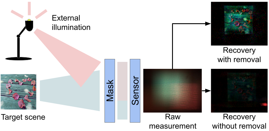
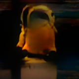
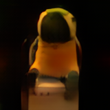
One source of noise/interference that has not been studied in lensless imaging is external illumination, i.e. light not emitted from the object of interest. This can take many forms and is unavoidable in practical settings, e.g. ambient lighting such as natural outdoor lighting or diffuse indoor illumination, and/or direct lighting such as from lamps. Most works ignore the influence of external illumination by performing measurements in a very controlled, dark environment such that only the object(s) of interest are emitting light: e.g. either displaying images on a screen or directly shining a light on the object(s) [6, 7]. These controlled environments can be very different from scenarios in which lensless cameras may be deployed, thereby limiting the practicality of lensless systems if they can only be used in such contexts. The challenge with external illumination is that the multiplexing property of lensless cameras causes unwanted sources to spread across the entire captured image, potentially drowning out signal from the object of interest, as visualized by Fig. 1.
Contributions: In this work, we theoretically show the sensitivity of lensless imaging to external illumination, and propose methods to address this practical issue. Concretely, we propose techniques that use an estimate of the external illumination within a physics-based machine learning reconstruction. Moreover, we open-source the first lensless dataset (25K examples) measured under varied lighting conditions [14], and our reconstruction code in LenslessPiCam [15].111lensless.readthedocs.io
II Background
II-A Modeling of Lensless Imaging
A lensless imaging system is typically modeled as a linear mapping between a scene of incoherent point sources and a system matrix [5]:
| (1) |
where and are the vectorized lensless measurement and scene intensity respectively, and is additive noise.
A common assumption for simplifying calibration and compute is to assume a shift invariant system, turning 1 into a 2D convolution with the on-axis point spread function (PSF) [1]. Using the convolution theorem, 1 can be written as a point-wise multiplication in the frequency domain. The PSF can be measured, e.g. with a white LED at far-field in a dark room, or simulated if the mask structure is known [7, 9].
II-B Sensitivity to Model Mismatch
Image recovery can be posed as an optimization problem:
| (2) |
where is a regularization function on the estimate image. This can be solved with an iterative algorithm (e.g. FISTA [2], ADMM [5]), Wiener filtering [4], or learned approaches [6, 7, 9]. However, these methods can be sensitive to mismatch in the system matrix , e.g. either the PSF estimate is noisy, or the shift invariant assumption is too simplistic. If we denote our estimate system matrix as where the deviation from the true system matrix is , our forward model can be written as:
| (3) |
Assuming the system is invertible and with spectral radius , applying direct inversion with yields [16]:
| (4) | ||||
| (5) |
A similar breakdown can be shown for each ADMM iteration, leading to an accumulation of errors over iterations [10].
II-C Robust Lensless Imaging
Considering the decomposition in Section II-B, robust lensless imaging needs to (1) minimize the model mismatch , (2) minimize the input noise , and/or (3) reduce the amplification of both. Previous works attempt to minimize in a data-driven fashion by learning the on-axis PSF [7, 8] or performing neural-network transformations of the PSF [9]. For reducing the input noise, a denoiser can be used prior to camera inversion [13]. Moreover, nearly all state-of-the-art methods apply a form of post-processing for perceptual enhancements [6, 7], which can also reduce the amplified error terms in Section II-B. For iterative algorithms, the intermediate outputs can be used to reduce the accumulating error [10].
III Methodology
In this section, we demonstrate lensless imaging’s sensitivity to external illumination and multiple approaches to address it. The noise in 1 can be further decomposed as:
| (6) |
where is additive noise at the sensor, and consists of illumination from external objects and ambient lighting that go through the imaging system’s mask.
Inserting 6 for in Section II-B yields:
| (7) |
Our objective is to reduce by making use of an estimate of the external illumination:
| (8) |
where is the error in the estimate. The estimate can be obtained by e.g. averaging over multiple video frames [17] or taking a measurement when the target object is not present. To obtain such an estimate, our approach is best suited for cameras that are installed at fixed locations, e.g. for surveillance.
III-1 Direction Subtraction
The simplest approach is to directly subtract the estimate prior to image recovery, i.e. , such that is amplified instead of 6:
| (9) |
While Section III-1 still has an error term associated with the external illumination, we expect that the is smaller than for a good estimate, such that the noise amplified by Section III-1 is smaller than the noise amplified by Section III, i.e. .
III-2 Learned Subtraction
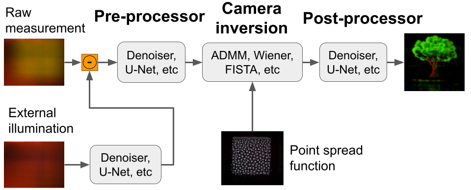
To reduce the error in the external illumination and thus in Section III-1, we can learn a neural-network transformation of , similar to previous approaches that input the PSF to a neural network to reduce model mismatch [9]. Fig. 2 shows our proposed architecture for incorporating external illumination removal into the lensless imaging pipeline. Prior to applying the pre-processor, the processed version of is subtracted from the measurement.
III-3 Concatenate External Illumination
The previous approach introduces a strong inductive bias by using a subtraction as the first (and only) operation between the measurement and the external illumination estimate. Alternatively, we can concatenate them as a single input to the pre-processor, such that the appropriate operations can be learned between the two. This is similar to FFDNet [18] and DRUNet [19], which concatenate a single-channel noise level map to the input image. In our case, we concatenate three-channel external illumination estimate for a six-channel input to the pre-processor.
IV Experiments
IV-A Hardware Setup
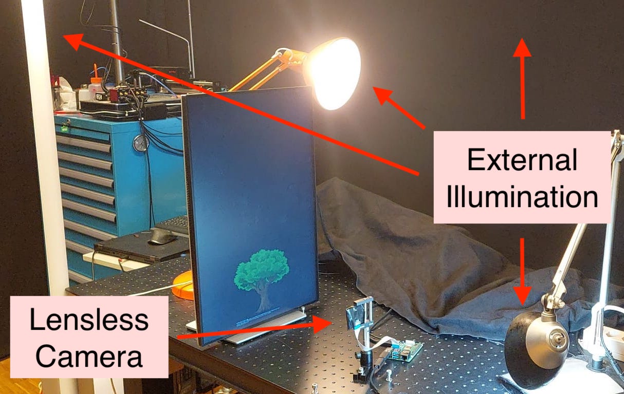
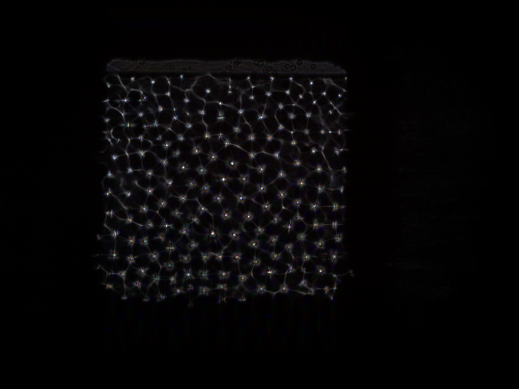
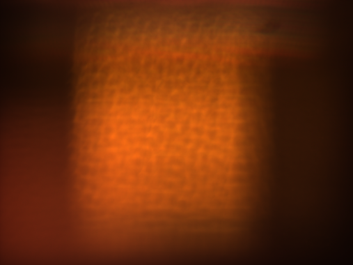
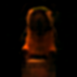
Our lensless camera and measurement setup can be seen in Fig. 3. A monitor is placed from the camera to project images, while our camera consists of a phase mask from a Raspberry Pi HQ sensor [20]. The phase mask (Fig. 4(a)) has a multi-focal pattern of size that has been fabricated using ultraviolet single-exposure photolithography [21]. The PSF can be seen in Fig. 4(b).
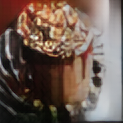
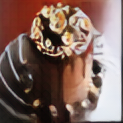
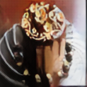
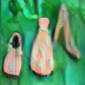
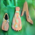
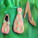
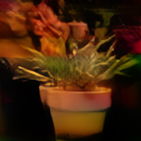
We collect a dataset of 25K images from the MirFlickr dataset [22] with a lensless camera and under multiple sources of external illumination: natural outdoor lighting, indoor (diffuse) ceiling lighting, and directional lamps.
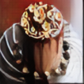
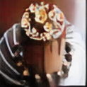
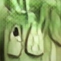
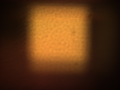
During dataset collection (over 10 days), as well as variations from outdoor lighting, we vary the lamp positions for measurements with different external illuminations: four different positions in the train set and three in the test set. For each image, we obtain two measurements: (1) the target scene on the screen and (2) the screen set to all-black. The latter serves as our external illumination estimate. The left-most column of Fig. 5 shows measurements in our test set with different lighting positions; the inset shows the external illumination estimate. A train-test split of 85-15 is used: 21.25K files for training and 3.75K files for testing. The dataset is open-sourced on Hugging Face [14].
| Measurement | Ground-truth | LeADMM + [6] | With learned subtraction | & [13] | & (concatenate) | TrainInv + [7] | & (concatenate) |
|
\stackinsetl-0.25cmt-0.25cm

|
\stackinsetl-0.25cmt-0.25cm

|
\stackinsetl-0.25cmt-0.25cm
|
\stackinsetl-0.25cmt-0.25cm
|
\stackinsetl-0.25cmt-0.25cm
|
\stackinsetl-0.25cmt-0.25cm
|
\stackinsetl-0.25cmt-0.25cm

|
\stackinsetl-0.25cmt-0.25cm
|
|
\stackinsetl-0.25cmt-0.25cm
|
\stackinsetl-0.25cmt-0.25cm

|
\stackinsetl-0.25cmt-0.25cm
|
\stackinsetl-0.25cmt-0.25cm
|
\stackinsetl-0.25cmt-0.25cm
|
\stackinsetl-0.25cmt-0.25cm
|
\stackinsetl-0.25cmt-0.25cm
|
\stackinsetl-0.25cmt-0.25cm
|
|
\stackinsetl-0.25cmt-0.25cm

|
\stackinsetl-0.25cmt-0.25cm

|
\stackinsetl-0.25cmt-0.25cm
|
\stackinsetl-0.25cmt-0.25cm
|
\stackinsetl-0.25cmt-0.25cm
|
\stackinsetl-0.25cmt-0.25cm

|
\stackinsetl-0.25cmt-0.25cm
|
\stackinsetl-0.25cmt-0.25cm
|
IV-B Reconstruction Approaches
All approaches can be understood with respect to the modular pipeline in Fig. 2. As baselines, we consider two camera inversions approaches: unrolled ADMM with learned parameters (LeADMM) [6] and fine-tuning the PSF for single-step inversion (TrainInv) [7]. With these camera inverters we either use a neural-network post-processor [6, 7], or both a pre- and post-processor [13]. To the baselines, we incorporate our proposed techniques from Section III to address external illumination. For a valid comparison, we limit the total number of neural network parameters to around 8.1M. To this end, all denoisers use the DRUNet architecture [19] with the number of intermediate channels set for a target number of parameters denoted in the subscript, e.g. refers to a pre-processor with around 4M parameters. For learned subtraction, a DRUNet with just 128K parameters is used for the external illumination and the pre-processor size is slightly reduced.
IV-C Training and Evaluation
PyTorch [23] is used for training and evaluation on an Intel Xeon E5-2680 v3 CPU and 4 Nvidia Titan X Pascal GPUs. Training is done with the AdamW optimizer [24] with , , , and weight decay of . A cosine decay learning rate schedule is used with an initial learning rate of , after a warm-up of of the training steps (for epochs and a batch size of ). Similar to previous work, our loss function is a sum of the mean-squared error and the learned perceptual image patch similarity (LPIPS) with VGG weights [25] between the reconstruction and the ground-truth :
| (10) |
Three metrics are used to evaluate image recovery quality: peak signal-to-noise ratio (PSNR), structural similarity index measure (SSIM), and LPIPS.
IV-D Results
When using LeADMM [6] for camera inversion (Tab. I and middle columns of Fig. 5), only using a post-processor results in blurring and loss of detail. Adding learned subtraction restores finer details and improves the metrics: increase and and relative improvement in SSIM and LPIPS. Using a pre-processor further improves performance, even without accounting for external illumination. The best performance is obtained with a pre-processor and the proposed subtraction/concatenation techniques. Using TrainInv [7] for camera inversion also benefits from the proposed techniques (Tab. II and last columns of Fig. 5). While worse than LeADMM, it has faster inference [13].
| Method | PSNR | SSIM | LPIPS |
| LeADMM+ [6] | 17.5 | 0.501 | 0.425 |
| With direct subtraction | 18.6 | 0.525 | 0.380 |
| With learned subtraction | 19.5 | 0.577 | 0.368 |
| +LeADMM+ [13] | 19.9 | 0.600 | 0.352 |
| With direct subtraction | 19.9 | 0.592 | 0.336 |
| With learned subtraction | 20.5 | 0.618 | 0.331 |
| Concatenate | 20.6 | 0.623 | 0.329 |
| Method | PSNR | SSIM | LPIPS |
| TrainInv+ [7] | 16.8 | 0.488 | 0.485 |
| With direct subtraction | 16.9 | 0.451 | 0.472 |
| With learned subtraction | 18.0 | 0.535 | 0.445 |
| +TrainInv+ [13] | 18.9 | 0.574 | 0.396 |
| With direct subtraction | 18.5 | 0.533 | 0.394 |
| With learned subtraction | 19.5 | 0.560 | 0.410 |
| Concatenate | 20.3 | 0.624 | 0.355 |
| Measurement | ADMM100 (direct sub) | LeADMM + [6] | & (concatenate) |
|
\stackinsetl-0.25cmt-0.25cm
|
 |
 |
 |
|
\stackinsetl-0.25cmt-0.25cm
|
 |
 |
 |
|
\stackinsetl-0.25cmt-0.25cm
|
 |
 |
 |
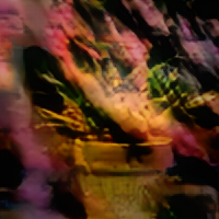
Fig. 6 shows reconstructions of real objects to show performance beyond images on a screen. Our approach improves contrast and is more robust to changes in lighting.
V Conclusion
We propose simple yet robust techniques for enabling lensless imaging under external illumination, improving the practicality of such systems beyond controlled setups. We theoretically show the adverse effects of external illumination to motivate our approaches, in which we subtract/concatenate an estimate of the illumination. We open source our implementations and a dataset measured in varied lighting conditions. One limitation is the assumption that the target object is not present when the external illumination is estimated. Source separation techniques [26] could be explore for scenarios where the target and external illumination need to be simultaneously recovered.
Acknowledgment
The authors thank Kyung Chul Lee for providing the fabricated mask for the lensless camera prototype.
References
- [1] Vivek Boominathan, Jacob T Robinson, Laura Waller, and Ashok Veeraraghavan, “Recent advances in lensless imaging,” Optica, vol. 9, no. 1, pp. 1–16, 2022.
- [2] Kristina Monakhova, Kyrollos Yanny, Neerja Aggarwal, and Laura Waller, “Spectral DiffuserCam: lensless snapshot hyperspectral imaging with a spectral filter array,” Optica, vol. 7, no. 10, pp. 1298–1307, Oct 2020.
- [3] Nick Antipa, Patrick Oare, Emrah Bostan, Ren Ng, and Laura Waller, “Video from stills: lensless imaging with rolling shutter,” in IEEE Int. Conf. on Computational Photography, 2019, pp. 1–8.
- [4] M. Salman Asif, Ali Ayremlou, Aswin Sankaranarayanan, Ashok Veeraraghavan, and Richard G. Baraniuk, “FlatCam: thin, lensless cameras using coded aperture and computation,” IEEE Transactions on Computational Imaging, vol. 3, no. 3, pp. 384–397, 2017.
- [5] Nick Antipa, Grace Kuo, Reinhard Heckel, Ben Mildenhall, Emrah Bostan, Ren Ng, and Laura Waller, “DiffuserCam: lensless single-exposure 3D imaging,” Optica, vol. 5, no. 1, pp. 1–9, Jan 2018.
- [6] Kristina Monakhova, Joshua Yurtsever, Grace Kuo, Nick Antipa, Kyrollos Yanny, and Laura Waller, “Learned reconstructions for practical mask-based lensless imaging,” Opt. Express, vol. 27, no. 20, pp. 28075–28090, Sep 2019.
- [7] S. Khan, V. Sundar, V. Boominathan, A. Veeraraghavan, and K. Mitra, “FlatNet: towards photorealistic scene reconstruction from lensless measurements,” IEEE Transactions on Pattern Analysis & Machine Intelligence, oct 2020.
- [8] Oliver Kingshott, Nick Antipa, Emrah Bostan, and Kaan Akşit, “Unrolled primal-dual networks for lensless cameras,” Opt. Express, vol. 30, no. 26, pp. 46324–46335, Dec 2022.
- [9] Ying Li, Zhengdai Li, Kaiyu Chen, Youming Guo, and Changhui Rao, “MWDNs: reconstruction in multi-scale feature spaces for lensless imaging,” Opt. Express, vol. 31, no. 23, pp. 39088–39101, Nov 2023.
- [10] Tianjiao Zeng and Edmund Y. Lam, “Robust reconstruction with deep learning to handle model mismatch in lensless imaging,” IEEE Trans. on Computational Imaging, vol. 7, pp. 1080–1092, 2021.
- [11] Stephen Boyd, Neal Parikh, Eric Chu, Borja Peleato, and Jonathan Eckstein, “Distributed optimization and statistical learning via the alternating direction method of multipliers,” Foundations and Trends® in Machine Learning, vol. 3, no. 1, pp. 1–122, 2011.
- [12] Joshua D. Rego, Karthik Kulkarni, and Suren Jayasuriya, “Robust lensless image reconstruction via PSF estimation,” in IEEE Winter Conf. on Applications of Comput. Vis., 2021, pp. 403–412.
- [13] Yohann Perron, Eric Bezzam, and Martin Vetterli, “A modular physics-based approach for lensless image reconstruction,” in IEEE Int. Conf. on Image Process., 2024.
- [14] Stefan Peters and Eric Bezzam, “MultiLens-Mirflickr-Ambient Dataset,” https://doi.org/10.57967/hf/2970 (Sep. 2024).
- [15] Eric Bezzam, Sepand Kashani, Martin Vetterli, and Matthieu Simeoni, “LenslessPiCam: A hardware and software platform for lensless computational imaging with a Raspberry Pi,” Journal of Open Source Software, vol. 8, no. 86, pp. 4747, 2023.
- [16] Yuesong Nan and Hui Ji, “Deep learning for handling kernel/model uncertainty in image deconvolution,” in IEEE Conf. on Comput. Vis. and Pattern Recog., 2020, pp. 2385–2394.
- [17] M. Piccardi, “Background subtraction techniques: a review,” in 2004 IEEE International Conference on Systems, Man and Cybernetics (IEEE Cat. No.04CH37583), 2004, vol. 4, pp. 3099–3104 vol.4.
- [18] Kai Zhang, Wangmeng Zuo, and Lei Zhang, “FFDNet: Toward a fast and flexible solution for CNN-based image denoising,” IEEE Transactions on Image Processing, vol. 27, no. 9, pp. 4608–4622, 2018.
- [19] Kai Zhang, Yawei Li, Wangmeng Zuo, Lei Zhang, Luc Van Gool, and Radu Timofte, “Plug-and-play image restoration with deep denoiser prior,” IEEE Transactions on Pattern Analysis and Machine Intelligence, vol. 44, no. 10, pp. 6360–6376, 2021.
- [20] “Raspberry Pi high quality camera,” www.raspberrypi.com/products/raspberry-pi-high-quality-camera (Sep. 2024).
- [21] Kyung Chul Lee, Junghyun Bae, Nakkyu Baek, Jaewoo Jung, Wook Park, and Seung Ah Lee, “Design and single-shot fabrication of lensless cameras with arbitrary point spread functions,” Optica, vol. 10, no. 1, pp. 72–80, Jan 2023.
- [22] Mark J Huiskes and Michael S Lew, “The MIR Flickr retrieval evaluation,” in Proceedings ACM Int. Conf. on Multimedia Information Retrieval, 2008, pp. 39–43.
- [23] Adam Paszke, Sam Gross, Soumith Chintala, Gregory Chanan, Edward Yang, Zachary DeVito, Zeming Lin, Alban Desmaison, Luca Antiga, and Adam Lerer, “Automatic differentiation in PyTorch,” NIPS Workshop Autodiff, 2017.
- [24] Ilya Loshchilov and Frank Hutter, “Decoupled weight decay regularization,” arXiv preprint arXiv:1711.05101, 2017.
- [25] Richard Zhang, Phillip Isola, Alexei A Efros, Eli Shechtman, and Oliver Wang, “The unreasonable effectiveness of deep features as a perceptual metric,” in IEEE/CVF Conf. Comput. Vis. and Pattern Recog., 2018.
- [26] Ganesh R Naik and Dinesh K Kumar, “An overview of independent component analysis and its applications,” Informatica, vol. 35, no. 1, 2011.