††thanks: These authors contributed equally to this work.††thanks: These authors contributed equally to this work.
Post- theory and its application to pseudogap in strongly correlated system
Hui Li
physicslihui@zju.edu.cnInstitute for Advanced Study in Physics and School of Physics, Zhejiang University, Hangzhou 310027, China
Yingze Su
School of Physics, Peking University, Beijing 100871, China
Junnian Xiong
School of Physics, Peking University, Beijing 100871, China
Haiqing Lin
hqlin@zju.edu.cnInstitute for Advanced Study in Physics and School of Physics, Zhejiang University, Hangzhou 310027, China
Huaqing Huang
huaqing.huang@pku.edu.cnSchool of Physics, Peking University, Beijing 100871, China
Dingping Li
lidp@pku.edu.cnSchool of Physics, Peking University, Beijing 100871, China
Abstract
The approximation is a widely used framework for studying correlated materials, but it struggles with certain limitations, such as its inability to explain pseudogap phenomena. To overcome these problems, we propose a systematic theoretical framework for Green’s function corrections and apply it specifically to the approximation. In this new theory, the screened potential is reconnected to the physical response function, i.e. the covariant response function proposed in Li et al. (2023), rather than using the RPA formula. We apply our scheme to calculate Green’s function, the spectral function, and the charge compressibility in the two-dimensional Hubbard model. Our scheme yields significant qualitative and quantitative improvements over the standard method and successfully captures the pseudogap behavior.
††preprint: APS/123-QED
Introduction.—
Green’s function determines the single-particle spectrum, band structure, energy, and other important properties. However, accurately calculating Green’s function in strongly correlated systems is one of the greatest challenges and crucial problems in condensed matter physics. One commonly used approach to evaluate Green’s function is the approximation by truncation of Dyson’s equationAltland and Simons (2010); Coleman (2015). In particular, the approximation is one of the most widely used approaches, which contains the screened effect in its self-energy, and it has been successfully applied in metals, semimetals, nanomaterials and so onHedin (1965); Leng et al. (2016); Aryasetiawan and Gunnarsson (1998); Golze et al. (2019a, b). However, it also suffers from some serious shortcomings, including the absence of satellite peaks in the spectrum, and the inability to describe the pseudogap in strongly correlated systemsReining (2018); Sun et al. (2021a).
The pseudogap, characterized by the depletion of electronic states in the normal state near the Fermi surface, is a phenomenon observed in many strongly correlated systems, including copper-oxide superconductors and unitary Fermi gases.Timusk and Statt (1999); Sadovskii (2001); Stewart et al. (2008); Haussmann et al. (2009); Kondo et al. (2009); Gaebler et al. (2010); Li et al. (2024). Understanding the pseudogap is widely considered crucial for unraveling the microscopic mechanisms underlying high-temperature superconductivity.
To address the limitations of the approximation, various extensions have been proposed, such as combing it with the dynamical mean-field theory (DMFT) Choi et al. (2016) or extending to higher-order vertex approximations in Hedin’s equation Takada (2001); Shishkin et al. (2007); Maebashi and Takada (2011); Romaniello et al. (2012); Grüneis et al. (2014); Chen and Pasquarello (2015); Kutepov (2016); Ren et al. (2015); Kutepov and Kotliar (2017); Pavlyukh et al. (2020); Kutepov (2022); Weng et al. (2023). Nevertheless, these attempts have yet to fully resolve the issues related to the pseudogap and other strongly correlated phenomena within the framework.
In this Letter, we propose a general framework to improve Green’s function of the existing many-body approximation theories, which we term the post theory. We apply this scheme to the approximation to obtain the post- theory, a significant advancement over the conventional theory. Our motivation arises from the violation of the intrinsic relationships for the high-order correlation functions in the original theories due to truncation, for example, the relation between the screened potential and the charge/spin correlation. In the theory, such a relation is violated due to the vertex approximation. In Ref. Li et al. (2023), we introduce the covariant theory to obtain physical charge/spin correlation functions, which preserve the fluctuation-dissipation theorem (FDT) Kubo (1966) and the Ward-Takahashi Identity (WTI) Peskin (1995). In our post- theory, we replace the screened potential in the Green’s function with the physical one, which is determined by the covariant response function.
To validate the post framework, we apply the post- approach to 2D Hubbard models to calculate Green’s functions and compare our results with those obtained from the Determinantal Quantum Monte Carlo (DQMC) method. Moreover, we use the Nevanlinna analytical continuation to calculate the spectral function, demonstrating that
the post- approach can indeed describe the pseudogap. Finally, we calculate the compressibility and compare it with DQMC results from Ref. Huang et al. (2019).
General formalism.
—For an arbitrary exact many-body theory, it can always be expressed as:
(1)
where is the Green’s function, is the n-th functional derivative to an external source .
Functional presents as Dyson’s equation Rosenstein and Li (2018); Fan et al. (2020); Sun et al. (2021b).
However, such equations cannot be exactly solved for most correlated systems because they are not closed (infinite hierarchy). Hence, we need approximations to make these equations solvable (for example, for all ). The approximate equations take the form after taking (named on-shell equations):
(2)
Eqs. (2) are closed and can be solved. The formations for may differ from in the exact theory. It should be pointed out that, the solutions of Eqs. (2) are “truncated” correlations, i.e. they are not “physical” because these correlations violate the definition . This feature leads to the “truncated” Green’s function being unable to obey some crucial relations for cumulants , for example, WTI and FDT Li et al. (2023). Now we propose the following formalism to calculate the physical correlations.
Next, we consider the Eqs. (2) with the source term , referred to as the off-shell equations. To obtain the physical correlation, we calculate the functional derivative with respect to in off-shell Eqs. (2) :
(3)
Here we denote , and call Eqs. (3) covariant equations, which are linear for and . The Eqs. (3) can be solved by taking the shell limit .
Similarly, the second-order functional derivative provides a set of linear equations about , , and one can evaluate . We can repeat this procedure to obtain all physical correlations . We should point out that the solutions of covariant equations are physical because they are defined through the functional derivative, satisfying Kubo’s formula automatically Kubo (1966) (relation between the response function and the correlation function).
The new Green’s function is proposed by replacing the in Eqs. (2) by the physical correlation :
(4)
The method to obtain presented above is called post theory for the approximation of Eqs. (2) in this article. The validity of the post framework can be verified by applying it to exactly solvable toy models (see
Supplemental Material (SM) for detailed calculations). Subsequently, we will consider its application to the approximation.
Hedin’s equations and equations for general action.—We start with a general Matsubara action form at finite temperature Aryasetiawan and Biermann (2008):
where are Grassmannian fields, are charge/spin operators and are Pauli matrices. The Greek letters like indicate the spin projection. The label is a generalized coordinate, containing the space coordinate , and the imaginary time coordinate , where and are the Boltzmann constant and thermal-dynamic temperature respectively. The symbol represents an integral over all space and time coordinates for a continuous system or a summation over all lattice and time coordinates for a discrete system. The two-body interaction is real symmetric, i.e., .
We introduce an external vector source coupled to the charge/spin operator , and obtain
the perturbed action
(5)
By virtue of the grand partition function ,
one can define the one-body Green’s functions as
(6)
presents for , and defines the functional integral measure. Due to the spin structure of the interaction, we denote the matrix in the spin space as
where is the Hartree propagator, which takes the form .
And is the effective potential. Here the vertex is obtained by . The screened potential here is defined by , and it can be simplified by introducing the polarization function as:
(9)
Hedin’s equations consist of Eqs. (8,9). It should be noted that there exists an exact relation between the charge/spin correlation and the screened potential
(10)
where we use the definitions of .
The simplest approximation for the vertex function results in the approximation with the following self-energy and polarization function:
(11)
(12)
One can solve the on-shell equations () to obtain the truncated Green’s function and screened potential .
It should be noted that according to Eq. (10), the screened potential is induced by the charge/spin correlation in the exact theory. However, the relation (10) is broken by the vertex approximation in the theory. By combining Eq. (10) and Eq. (12), we can find the screened potential in the equations is induced by the RPA correlation :
(13)
is unphysical since it violates the basic definition , therefore violates the WTI and the FDT. So our goal is to reconnect the screened potential to the physical correlation function in the framework.
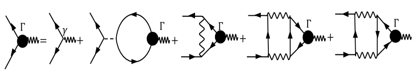
Figure 1: The Feynman diagram of the full vertex function for translational invariant systems in the momentum space. The dashed line denotes the interaction, the wave line denotes the , and the solid line represents the in the equations.
Post- approach.—In Ref.Li et al. (2023), we proposed the covariant (cGW) approach to calculate charge/spin correlation functions with the Feynman diagrams as shown in Fig. S1, which can both preserve the FDT and the WTI within the framework. In the covariant scheme, all correlation functions should be defined as the response of the physical quantity in the presence of an external potential in each many-body theory. It is consistent with the approach for calculating the high-order correlation in the post framework.
Now we calculate the post Green’s function by using the covariant charge/spin correlation and the physical screened potential, which is the application of the post framework above in the , named post-. To obtain Green’s function for the post-, the following steps are used:
1.
Solve the equations to get the truncated Green’s function , unphysical screened potential , and the Hartree propagator .
2.
Calculate the covariant vertex using and , obtaining Li et al. (2023).
3.
Compute the physical screened potential:
(14)
4.
Use to evaluate the post Green’s function:
(15)
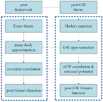
Figure 2: The flow chart of the general post framework and the post- theory. For the exact theory part, Hedin’s equation corresponds to the Eqs. 1 within the general framework. For the truncated equations part, equations correspond to Eqs. (2). For the covariant part, Eqs. (3) is represented as Feynman diagrams in Fig. S1, and covariant correlation and physical screened potential are provided. In the post Green’s function calculation part, Eqs. (15) is the specific form of Eq. (4) in the post- approach.
To demonstrate the relation between the post framework and the post- approach, we present the comparison in Fig.(2).
The Hubbard model is universally acknowledged as a basic model of the strongly correlated systems for high-temperature superconductivity and is expected to describe pseudogap physics(Qin et al. (2022) and references therein). Therefore, we apply the post- approach to the 2D () single-band Hubbard model and test its performance by directly comparing them with quantum Monte Carlo results.
Implementation in the Hubbard model.
—Here the post- is used to calculate the Green’s function, its spectral function, and the charge compressibility. The Hubbard Hamiltonian with the spin-dependent interaction takes the form Schäfer and Toschi (2021):
(16)
where we use the relation to rewrite the Hubbard interaction form , which can preserve the symmetry explicitly in the many-body calculation. Here creates an electron with spin at lattice site . denotes the spin-resolved density operator. The hopping amplitude between sites and equals for the nearest neighbors and for the next nearest neighbors. Unless otherwise stated, the default values for the hopping amplitude in this paper are , . is the on-site interaction and is the chemical potential.
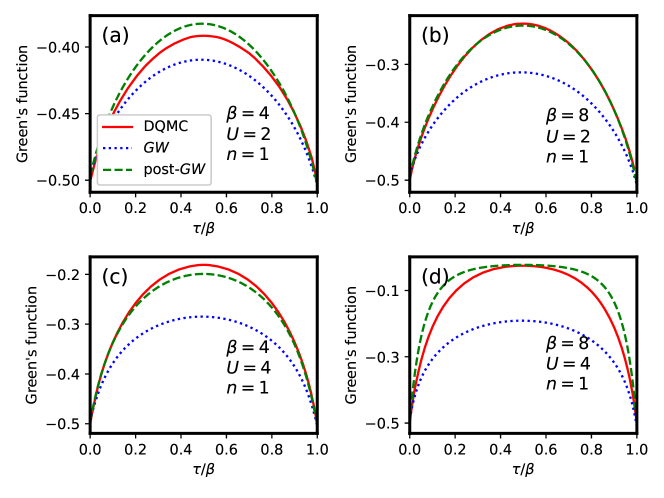
2D Green’s function in the Hubbard model.—We simulate square clusters by , post-, and DQMC, which is a well-known numerical exact method at half-filling without the fermion sign problem. Green’s functions at the anti-nodal point for the parameters , at half-filling in imaginary time are plotted to compare their accuracy directly. Figure 3 shows that, for all these parameters, the post- approach significantly improves Green’s function, even for the immediate coupling , where the traditional is regarded as performing poorly.
Figure 3: Green’s functions at the antinodal point in imaginary time space for a lattice at half-filling for DQMC, , and post- with different parameters:(a),(b),(c),(d).
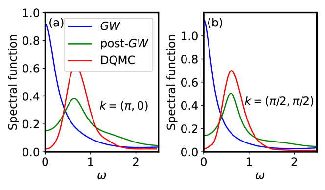
To provide robust evidence for the existence of the pseudogap for the immediate at the low temperature in the post- theory, we calculated the Green’s function on an lattice at , and obtained the spectral function by Nevanlinna analytic continuation Fei et al. (2021).
In Fig. 4, a comparative analysis with the spectral function derived from DQMC with the maximum entropy method as presented in Ref. Rost et al. (2012) reveals that, in contrast to the poor results of the , the post- methodology successfully identifies the pseudogap at both the nodal point and antinodal point , consistent with the peak positions exposed by DQMC + Maximum Entropy curves. Therefore, the post- approach effectively captures the main features of the pseudogap.
Figure 4: Comparison of the results of the spectral functions by , post- and DQMC + Maximum Entropy from Ref. Rost et al. (2012) for cluster at , and half-filling at different momenta: (a) , (b) .
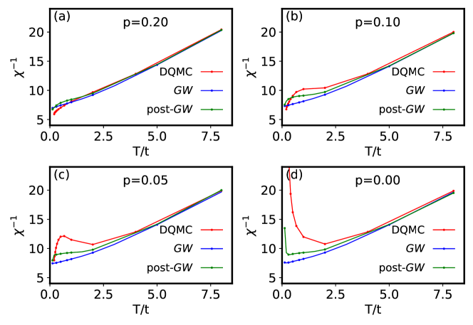
To further investigate the performance of the post- approach on the two-body correlation functions, we apply the new approach to the calculation of the charge compressibility and compare it with the exact DQMC results Huang et al. (2019), where the parameters are taken as cluster, , . The charge compressibility plays an important role in the transport properties of the Hubbard model through the Nernst-Einstein relation, and the doping dependence of the inverse compressibility has similar features as the conductivity. Fig. S4 shows that the original agrees well with the DQMC in the high-temperature region, but differs from the DQMC qualitatively at low temperatures as the hole doping decreases. However, the post- curves not only are very close to the DQMC curves at high temperatures but also have the same qualitative characteristics as the DQMC at low temperatures with small hole doping . In particular, in the half-filling case, the DQMC results show that the inverse compressibility has an anomalous increase as the temperature decreases, and post- accurately captures such property.
Figure 5: Inverse charge compressibility calculated by , post- and DQMC from Ref. Huang et al. (2019) at different dopings. (a) , (b) , (c) , (d) ,
Conclusions.—In summary, we propose a theoretical framework for improving Green’s function in many-body approximation theories, termed post theory in this article, and apply it to the approximation, resulting in the post- method. This general framework is based on replacing unphysical higher-order correlations in the self-energy formula with covariant correlations. Specifically in the post- approach, we replace the RPA charge/spin correlation in the screened potential (13) with the corresponding covariant correlation functions.
We apply the post- approach to calculate the imaginary-time Green’s function, spectral function, and charge compressibility in the 2D Hubbard model. By comparing with the original and the exact DQMC results, it is found that post- can give significantly better results than in both qualitative and quantitative aspects for various physical quantities. In particular, our spectral function calculations reveal that the post- approach can capture the pseudogap, which indicates that the framework is not incapable of describing the physics of the pseudogap but only needs suitable refinement. We can also apply the post- to the 3D Hubbard model, which was recently experimentally studied in the cold atom system Shao et al. (2024), and observe the pseudogap phase which is referred to as the paramagnetic Mott state.
In the future, this framework can be expanded to investigate a wide range of correlated systems, including those exhibiting pseudogap phenomena. For example, in the unitary fermion gas, a superconducting pseudogap exists above the phase transition temperature Stewart et al. (2008); Haussmann et al. (2009); Gaebler et al. (2010); Li et al. (2024). Furthermore, the post framework has the potential to enhance the accuracy of various many-body approximation methods, making it a versatile tool for future research in strongly correlated physics.
Acknowledgements.
This work is supported by the National Natural Science Foundation of China (Grant No.12174006 of Prof. Li’s fund) and the High-performance Computing Platform of Peking University. H.H. acknowledges the support of the National Key R&D Program of China (No. 2021YFA1401600), and the National Natural Science Foundation of China (Grant No. 12074006 and 12474056). The authors are very grateful to B. Rosenstein, Tianxing Ma, Hong Jiang, Xinguo Ren, Changxiao Li, Wei Wang, and Sheng Yang for valuable discussions and help in numerical computations.
Combining Eqs.(11,14), one arrives at the following equation
(18)
which can be rewritten as:
(19)
The inverse of used above is defined by:
(20)
So, with functional derivative, we can derive the following set of generalized Hedin’s equations:
(21)
The corresponding equations can be obtained by simplification of the vertex functions:
(22)
The polarization function and the self-energy then becomes:
(23)
(24)
S2 Covariant theory
For the generalized Hartree approximation, which only contains Hartree self-energy in Eq (10), the two-body correlation function obtained by RPA formula can preserve the FDT and WTI (the vertex at the two-body level only contains the first two diagrams in Fig. S1). However, the higher-order approximation, such as , cannot preserve both the FDT and the WTI when using the RPA formula to calculate the two-body correlation.
According to the FDT, the two-body correlation functions should be defined as the response of the physical quantity in the presence of an external potential, which we refer to as the covariant scheme. The scheme for calculating a general connected two-body correlation function within the framework, where are binary composite operators, is formulated as follows.
First, one adds the corresponding source term to the action, and the correlation can be obtained by . Then, write down the off-shell equations (keep ), and calculate the functional derivative of the equations with respect to . Finally, let the source tend to to obtain the on-shell results. Although we restrict our discussion to the , this scheme can also be applied to different many-body approaches.
We consider the calculation of a generally connected two-body correlation function
,
where are local binary operators and take the form
(25)
The expression for the kernel depends on the operator . As for the spin operator, the kernel for is:
(26)
First, add an external local source coupled
to the operator and thus the perturbed action becomes
(27)
The additional term
is explicitly expressed as
(28)
Note that the additional term can be regarded as a variation of the
term:
(29)
Figure S1: The Feynman diagram of the full cGW vertex function in Eq. (30) for translation invariant systems.
The functional derivative of the off-shell equations with respect to the external source leads to the covariant (cGW) equations. The equation involves the full vertex function , which consists of 5 terms shown in Fig. S1:
(30)
Here, the bare vertex depends on the operator , and is calculated through
(31)
In the charge/spin response case, , the bare vertex takes the form . The “bubble” vertex is induced by the Hartree self-energy, i.e. , and takes the form:
(32)
Note that the conventional random-phase-approximation-like (RPA) formula only consists of the first two terms in Eq. (30).
The Maki-Thompson-like (MT) vertex and two distinct Aslamazov-Larkin-like (AL) vertices are induced by the self-energy, i.e., , representing the vertex corrections beyond the RPA, and take the form:
(33)
(34)
(35)
Finally, let and solve the self-consistent equations (30,31,32,33,34,35) to obtain the full vertex function .
Since the average is a function of the Green’s function , the two-body correlation function can be obtained by the vertex :
(36)
For example, when calculating the spin-spin correlation , the above equation can be simplified as:
(37)
Such response functions satisfy the FDT by definition, and the preserving of the WTI is proven in the next subsection.
S3 Implementation in the two-dimensional Hubbard model
S3.1 Fourier transformation for a translational invariant lattice
For a lattice with the translation symmetries, we use the discrete
Fourier transformation to simplify our equations. The Fermionic array
takes the form
(38)
and the Bosonic array takes the form
(39)
Here the transformation kernels and
are defined as
(40)
(41)
respectively. Here ,
and takes the integer value from to . Note that
the transformation of the -term is
(42)
with the non-interacting dispersion.
For the two-dimensional Hubbard model,
with the nearest-neighbor hopping strength.
S3.2 and covariant equations in Fourier space
Note that the one-body Green’s function and the self-energy
are Fermionic arrays, and the dynamical potential
and the polarization are Bosonic arrays. It is
easy to derive the equations in Fourier space
(43)
To derive the covariant equations in Fourier space, we first make
ansatz for the vertex function
(44)
Then one obtains
(45)
The bare vertex is
(46)
The bubble vertex is
(47)
The MT vertex is
(48)
The two AL vertices are
(49)
(50)
The diagrammatics for these vertices are presented in Fig. S1.
Note that in the random phase approximation (RPA), the RPA vertex
is given by
(51)
The RPA formula is usually used to calculate the density-density or
spin-spin correlation functions. In the Bethe-Salpeter equation approach,
the MT vertex is taken into account, but the AL vertices are neglected.
S3.3 and covariant equations for the 2D Hubbard model
For the 2D Hubbard model, takes the
form and
takes the form with taking values of .
To find the paramagnetic solutions, we can make the ansatz
(52)
and
(53)
The equation is then simplified as
(54)
The simplification of the covariant equations related to the species
of correlation functions. We take the spin-spin correlation function
as an example here. The spin-spin correlation function
relates to the vertex function through
(55)
Here refers to the vertex function corresponding
to the spin operator . By the ansatz , the spin-spin correlation function , and the equation for the vertex function is simplified as
(56)
with the bare vertex , the “bubble”
vertex
(57)
the MT vertex
(58)
and two AL vertices
(59)
(60)
S3.4 The Details for the Post- theory for Fermionic Toy Model
S3.4.1 Fermionic Toy Model and the Exact solution
Our starting point here will be the following “free energy” as a function of the Grassmannian variable :
(61)
Here, represents “couplings” for the Hubbard-like interaction, and the external source will be used to calculate correlations and derive Hedin’s equation. The exact partition function is:
(62)
According to the properties of the Grassmannian variables, we can rewrite the exponential term as
(63)
So the partition function can be evaluated exactly:
(64)
Here we use the relation:
(65)
Similarly, we can obtain the exact Green’s function:
(66)
S3.4.2 Hedin’s equation and the equations
Firstly, we write a more general action
(67)
where , , and in the toy model. Therefore, The partition function and the Green’s function takes the form:
(68)
(69)
To construct the Hedin’s equation, we need to introduce the source term in the action:
(70)
The invariance of the functional integral measure under the infinitesimal variation of field yields:
(71)
Then one can obtain the Dyson - Schwinger equation
(72)
One can use
(73)
to decompose the high-order correlations. Then one can rewrite the Eq. (72) as:
(74)
Here the Hartree propagator is defined as
(75)
and the density-weighted effective potential is:
(76)
To obtain the Hedin’s equation, we need to introduce the vertex function
(77)
and the screened potential
(78)
With the definition of the effective potential and the vertex , the screened potential can be written in terms of the Green’s function and vertex:
(79)
Combine Eq. (74,78,76,75,77), one can obtain the Hedin’s equation:
(80)
One can fine the exact relation between the screened potential and the high-order correlation :
(81)
The lowest-order approximation would lead to the equations, whose self-energy and screened potential take the form:
(82)
(83)
Here we use label to denote that the equations are ”truncated”, not exact. And the equations can be explicitly written as:
One can notice that the equations here can also be applied to lattice systems, like the Hubbard model if the label contains the time, space coordinates, and other freedom.
S3.4.3 Post- Equations for the Toy Model
According to the post framework, the high-order correlations should be recalculated to be ”physical”. Here, the only high-order correlation function in the equations is density correlation , which is hidden in the screened potential. So what we should do, is calculate the” physical” to obtain the ”physical” screened potential .
Here we use the source term in the original action again. According to our covariant framework, we need to add the source to the free term in the action:
(84)
Using the new free term , we can obtain the equations with a non-zero source directly, called off-shell equations. Then the functional derivative over the source in off-shell equations would give the covariant two-body vertex with the definition . The covariant equations are:
(85)
Solving these covariant equations, one can obtain the vertex , and the correlation can be calculated through:
(86)
Such defined by functional derivative is the ”physical” correlation function due to the Kubo formula. Then, we use the Eq. (81) to obtain the renormalized screened potential:
(87)
Finally, we can simulate the Green’s function for the post-GW:
(88)
The key procedure here is using the physical correlation to calculate the post-screened potential .
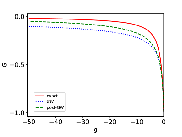
We compare the post- Green’s function with the and from the theory. Fig. (S2) shows that Green’s function of the approximate theory is much closer to the exact result after the post correction. The results from this toy model can preliminarily show the validity of the post theory and we will consider a more complex model subsequently.
Figure S2: Green’s function obtained by different approaches for an exact solvable model: exact solution (red solid), (blue dotted), post- (green dashed).
S4 Benchmark Results for chemical potential dependence of the particle density
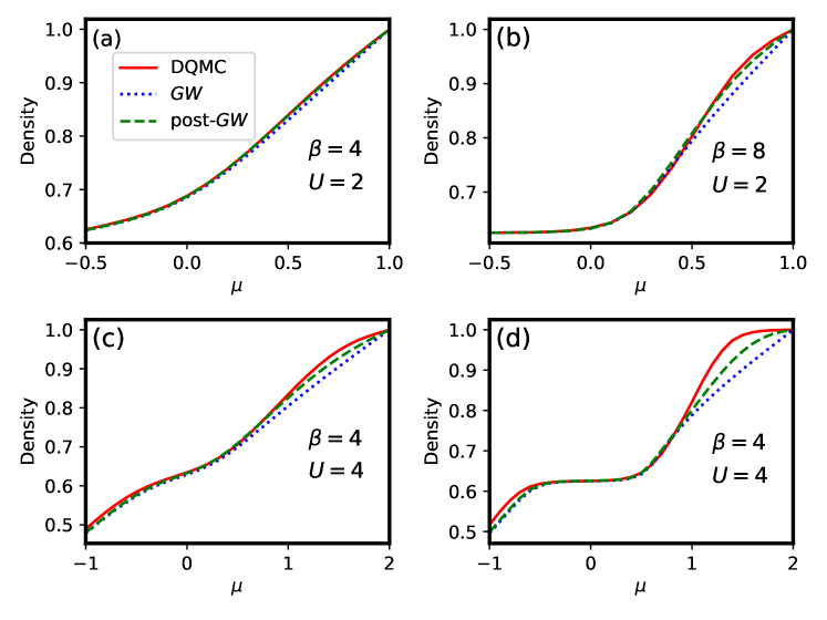
We study the chemical potential dependence of the particle density obtained from the post- Green’s function . Fig. S3 shows that
the original method deviates substantially from the exact DQMC results when the hole doping , while the post- can significantly correct this deviation in this region. In particular, in Fig. S3(d), where the DQMC result shows a plateau near half-filling indicating a Mott-Hubbard gap phase due to strong antiferromagnetic fluctuation, only post- can capture this feature, while fails obviously.
Figure S3: The chemical potential dependence of the particle density for DQMC, and post- at different parameters (a),(b),(c),(d).
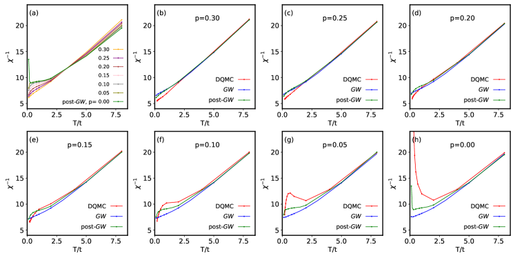
S5 Benchmark Results for charge compressitibility
To provide a more comprehensive analysis of the post- approach on the charge compressibility , we add more detailed results in Fig. S4. As shown in Fig. S4, the original method aligns well with the DQMC results at high temperatures but diverges qualitatively at lower temperatures as the hole doping decreases. In contrast, the post- approach not only closely matches the DQMC curves at high temperatures but also maintains similar qualitative features to the DQMC results at low temperatures, particularly when the hole doping .
Figure S4: Inverse charge compressibility calculated by , post- and DQMC simulations. (a) the curves of the post- at different dopings. (b) (h) The comparisons of the , post-, and DQMC at dopings .