Active Perception with Initial-State Uncertainty: A Policy Gradient Method
Abstract
This paper studies the synthesis of an active perception policy that maximizes the information leakage of the initial state in a stochastic system modeled as a hidden Markov model (HMM). Specifically, the emission function of the HMM is controllable with a set of perception or sensor query actions. Given the goal is to infer the initial state from partial observations in the HMM, we use Shannon conditional entropy as the planning objective and develop a novel policy gradient method with convergence guarantees. By leveraging a variant of observable operators in HMMs, we prove several important properties of the gradient of the conditional entropy with respect to the policy parameters, which allow efficient computation of the policy gradient and stable and fast convergence. We demonstrate the effectiveness of our solution by applying it to an inference problem in a stochastic grid world environment.
I INTRODUCTION
This paper studies the synthesis of an active perception strategy that maximizes the transparency of an initial state in a stochastic system given partial observations. We introduce a set of active perception actions into the system modeled as a hidden Markov model (HMM) such that the emission at a given state is jointly determined by the state and a perception action. The goal is to compute an active perception strategy that maximizes the information leakage about the initial state given observations , which is measured by the negative conditional entropy .
The contributions of this work are summarized as follows: First, we prove that active perception planning to minimize the conditional entropy cannot be reduced to a partially observable Markov decision process (POMDP) with a belief-based reward function. Leveraging a variant of observable operators [9], we develop an efficient algorithm to compute the posterior distribution given a perception policy. Additionally, it is shown that the policy gradient of conditional entropy depends only on the posterior distribution and the gradient of the policy with respect to its parameters. We prove that the entropy is Lipschitz continuous and Lipschitz smooth in the policy parameters under some assumptions for policy search space and thus ensure the convergence of the gradient-based planning. Finally, we evaluate the performance in a stochastic grid world environment.
Related Work Active perception [4] is to gather information selectively for improving the task performance of an autonomous system. The applications of active perception range from object localization [2], target tracking [5, 16] to mission planning for surveillance and monitoring [11, 6]. Information-theoretic metrics are introduced as planning objectives in various active perception problems. One approach [7, 3] to active perception is to formulate a partially observable Markov decision process (POMDP) with a reward function that depends on the information state or the belief of an agent. For example, in target surveillance, a patrolling team is rewarded by uncertainty reduction of the belief about the intruder’s position/state. In intent inference, the authors [14] used the negative entropy of the belief over the opponent’s intent as a reward and maximized the total reward for active perception.
Besides active perception, several studies have explored decision-making with information-theoretic objectives. In [12], the authors introduce a method for obfuscating/estimating state trajectories in POMDPs and show that the causal conditional entropy of the state trajectory given observations and controls can be reformulated as a cumulative sum, allowing the use of standard POMDP solvers. The work [15] develops a method to maximize the conditional entropy of a secret variable in an MDP to a passive observer. Another work [13] proposes entropy maximization in POMDPs to minimize the predictability of an agent’s trajectories to an outside observer. In both cases, the planning agent controls the stochastic dynamics and the observer is passive. In comparison, this paper studies the dual problem when the control system is autonomous but the observer is active. Thus, the observer’s policy is restricted to be observation-based. Unlike [13] where the goal is to maximize the sum of the conditional entropy of current states given the historical states, our goal is to maximize the information about some past state (initial state) given the observations received by the observing agent. This problem has important applications in intent recognition and system diagnosis [10].
II PRELIMINARIES AND PROBLEM FORMULATION
Notation The set of real numbers is denoted by . Random variables will be denoted by capital letters, and their realizations by lowercase letters (e.g., and ). A sequence of random variables and their realizations with length are denoted as and . The notation refers to the -th component of a vector or to the -th element of a sequence , which will be clarified by the context. Given a finite set , let be the set of all probability distributions over . The set denotes the set of sequences with length composed of elements from , and denotes the set of all finite sequences generated from . The empty string in is denoted by .
We introduce a class of active perception problems where the agent cannot control the dynamical system but can select perception actions to monitor it in order to infer some unknown state variables. The class of perception actions can be the choices of sensors to query in a distributed sensor network or the choices of poses for cameras with a limited field of view (FoV).
Definition 1.
An HMM with a controllable emission function is a tuple where 1. is a finite state space. 2. is a finite set of observations. 3. is a finite set of perception actions. 4. is the probabilistic transition function. 5. is the emission function (observation function) that takes a state and a perception action , outputs a distribution over observations. 6. is a random variable representing the initial state. The distribution of is denoted by . And denotes the set of initial states.
Definition 2.
A non-stationary, observation-based perception policy is a function that maps a history of observations to a distribution over perception actions.
Definition 3.
A finite-state, observation-based perception policy with deterministic transitions is a tuple where 1. is a set of memory states. 2. are a set of inputs and a set of outputs, respectively. 3. is a deterministic transition function that maps a state and an input to a next state . 4. is a probabilistic output function. 5. is the initial state.
Given a sequence of observations, the non-stationary policy directly outputs a distribution . A finite-state policy first computes the reached memory state and then outputs a distribution over actions. In both cases, we can treat as a function that maps to a distribution over actions and write as the probability of taking action given observations . When there is no observation, i.e., before the initial observation is made, the agent selects a perception action according to . If is a finite-state policy, then we can further obtain because .
For a given HMM , a perception policy induces a discrete stochastic process , where and are the underlying hidden state and observation at the -th time step, and
when the perception policy is understood from the context, we write instead of for clarity.
The conditional entropy of given is defined by
The conditional entropy measures the uncertainty about given knowledge of . A lower conditional entropy makes it easier to learn from observing a sample of .
For any finite horizon , the agent’s partial observation about a path in the HMM includes a sequence of observations and a sequence of perception actions. We denote the agent’s information by . When the length of is clear from the context, we omit the subscript and use to denote the sequence. In the following, we refer to as an observation sequence with the understanding that it is the joint observation and perception action sequence.
Problem 1.
Let an HMM and a finite horizon be given. Let be a policy space. Compute an active perception policy that minimizes the conditional entropy of the initial state given the partial information induced by . That is,
where is the joint probability of starting from and observing under the policy and is the conditional probability of starting from given observation .
Remark 1.
A constrained formulation to minimize entropy given a bounded perception cost can also be formulated. Because policy gradient methods [1] for optimizing a cumulative reward/cost are well-understood, we focus on solving this entropy minimization problem and expect that only a small modification to the gradient computation is needed to minimize a weighted sum of the conditional entropy and the expected total cost of perception actions.
III MAIN RESULT
First, we show that the problem cannot be reduced to a -POMDP [3] which is a POMDP with a belief-based reward. Given observations and a perception policy , the belief about is the posterior distribution .
Proposition 1.
There is no belief-based reward such that .
Proof.
Suppose, by way of contradiction, such a belief-based reward function exists. Then, . We show that it is possible to reach the same belief with two different observations and , but . Consider an example of HMM where the initial state can be either or with a prior distribution ; namely, the initial belief is given by . If , the next state will always emit an observation . If , the next state will always emit an observation . Thus, if is observed, then ; if is observed, then . The reward regardless whether or is observed. After reaching state , the system reaches next and yields some observation . The belief does not change, i.e., because the initial state is known with certainty. However, based on the formula , which is different from . A contradiction is established. ∎
In the next, we develop a policy gradient method to solve Problem 1. Consider a class of parametrized (stochastic) policies . We denote by the stochastic process induced by a policy , and the corresponding probability measure.
For a given parameterized policy , we denote by the set of possible observations under the perception policy . The gradient of is given by
| (1) | ||||
In the following, Propositions 5 and 4 will allow us to further simplify the computation of gradient.
To derive the results, we introduce the observable operator augmented with perception actions. The observable operator [8] has been proposed to represent a discrete HMM and used to calculate the probability of an observation sequence in an HMM using matrix multiplications.
Let the random variable of state, observation, and action, at time point be denoted as , respectively. Let be the flipped state transition matrix with
For each , Let be the observation probability matrix with .
Definition 4.
Given the HMM with controllable emissions , for any pair of observation and perception action , the observable operator given perception actions is a matrix of size with its -th entry defined as
which is the probability of transitioning from state to state and at the state , an observation is emitted given perception action . In matrix form,
Proposition 2.
The probability of an observation sequence given a sequence of perception actions , can be written as matrix operations,
| (2) |
In addition, for a fixed initial state ,
| (3) |
where is a one-hot vector which assigns 1 to the -th entry.
Proof.
To compute the gradient , we will need the value of . We start by calculating the probability of an observation sequence in .
Proposition 3.
The probability of a sequence of observations and perception actions in can be computed as follows:
| (4) |
where is the initial empty observation.
Proof.
By the product rule of probability and causality, we can write the probability in the form,
| (5) |
For any , based on the multiplication rule of probability, we can decompose the conditional probability as
| (6) |
Note that the probability of observing given the sequence of actions and past observations is independent from the policy . And the conditional probability is derived as
| (7) |
where (i) is because 1) the probability of observing is determined by state and perception action given the emission function ; and 2) the probability of reaching state at the -th time step does not depend on the perception action when the action sequence is fixed, which can be calculated by equation (2). The equality is established by the definition of observable operators and Proposition 2. Substituting (7) into (6) and rewrite (5),
| (8) | ||||
which can be computed efficiently using the matrix operators for calculating . ∎
For a fixed initial state , the result of (4) becomes
| (9) |
where the calculation of term is given in (3).
Numerical issues may arise in computing and because the probabilities can be close to 0 for a relatively long horizon . We can avoid these numerical issues by taking the logarithm of both sides of equation (9). The following properties further show the gradient calculation can be simplified.
Proposition 4.
Given , the gradient of can be computed as
| (10) | ||||
which is invariant with respect to the initial state .
Proof.
Proposition 5.
For any , the gradient of the logarithm of the posterior probability with respect to is 0, i.e., Further, when ,
Proof.
First, using the Bayes’ rule,
Taking the logarithm on both sides:
and then taking the gradient on both sides with respect to ,
From Proposition 4, we derive because and is a constant. Furthermore, because , when but , we can derive that . ∎
Theorem 1.
The gradient of the conditional entropy w.r.t. the policy parameter is
| (12) |
Proof.
The conditional entropy is given by:
When computing the gradient using (LABEL:eq:HMM_gradient_entropy), the terms in the summation corresponding to vanish. Let be the set of initial states from which an observation is possible. Then,
From Proposition 5, the gradient when . Thus, we have
| (13) | ||||
where the expectation is taken with respect to the stochastic process of observations induced by the perception policy . Note that can be computed using (10). ∎
Next, we show the convergence of a gradient-descent method under a common assumption of the policy space.
Assumption 1.
For any time step , for any , both and are bounded.
Theorem 2.
Under Assumption 1, the entropy is Lipschitz-continuous and Lipschitz-smooth in .
Proof.
We prove the theorem by showing that the gradient and Hessian are both bounded. Referring to (13), by Jensen’s inequality, we obtain
| (14) |
The results of Proposition 4 show that
| (15) |
which is bounded given Assumption 1 and the triangle inequality. Due to the boundedness of and , the gradient is also bounded because where . Next, consider the Hessian
| (16) | ||||
where the last equality is because and thus by Proposition 5. Further, when is bounded for all , , and ,
| (17) |
is bounded. Thus, is bounded by the triangle inequality. Combining (14) and (17), with similar reasoning for the boundedness of the gradient, it holds that is bounded. ∎
To obtain the locally optimal policy parameter , we initialize a policy parameter and carry out the gradient descent. At each iteration ,
| (18) |
where is the step size. When using the gradient descent algorithm to compute the optimal , it may be computationally expensive to compute by enumerating all possible observations . A sample approximation is employed such that at each iteration, we collect sequences of observations , and compute
IV EXPERIMENTS
Consider a stochastic grid world environment (Fig. 1) with three types of robots, each starting from different positions to reach specific goals (flags). The blue robot (type 1) starts at , the red (type 2) at , and the green (type 3) at . In line with standard grid world dynamics, each robot has a 20% chance of moving to one of the two nearest cells instead of the intended direction. Robots hitting walls or boundaries remain in place. Their policies are computed to maximize the probability of reaching their goals from their starting positions.
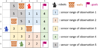
The environment has five sensors, each with a distinct range. The observer can query only one sensor at a time. For sensor , if a robot is within its range and the observer queries it, the observer receives observation with 90% probability and a null observation (“n”) with 10% probability (false negative). Otherwise, the observer also receives a null observation.
We consider finite-state perception policy (Def. 3): Given an integer , the state set are the set of observations with length . For each , is defined such that 111 is the last symbols of string if or itself otherwise. is the last (up to) observations after appending the observation to . The probabilistic output function is parameterized as, where is the policy parameter vector. Given observations , the policy . The softmax policy satisfies Assumption 1 and is differentiable. In the experiments, we set the length of memory .
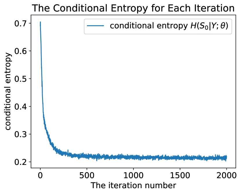
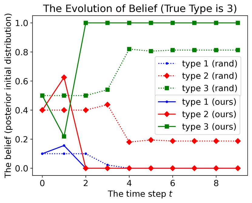
The initial distribution is for type 1, type 2, and type 3, respectively. Figure 2(a) illustrates the convergence of the policy gradient 222We sample trajectories and set the horizon for each iteration. The fixed step size of the gradient descent algorithm is set to be . We run iterations on the 12th Gen Intel(R) Core(TM) i7-12700, the average time consumed for one iteration is seconds.. When the algorithm converges, the conditional entropy approaches approximately . This indicates that the observations provide substantial information about the robot’s type on average.
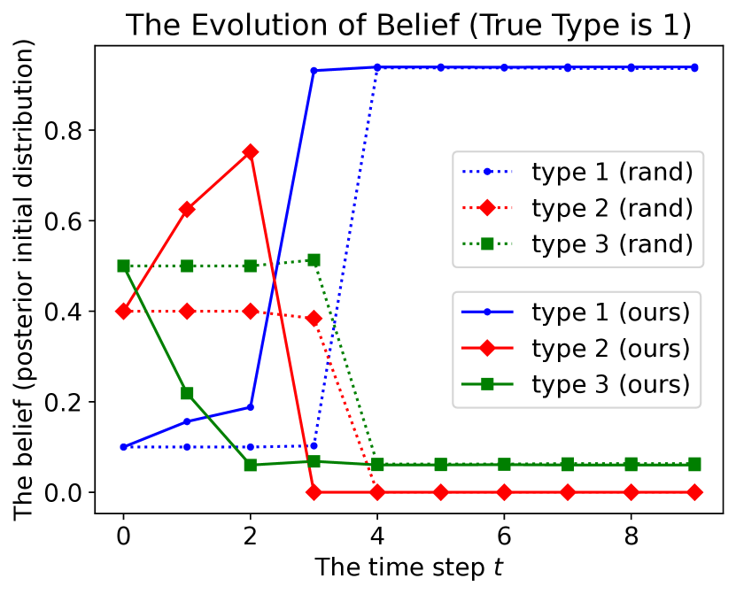
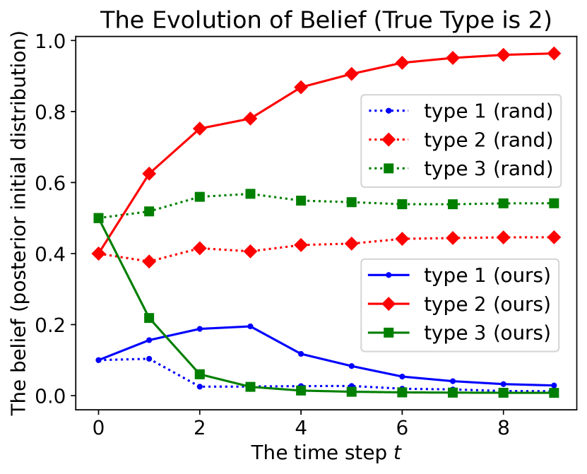
To provide an intuitive understanding, we use the computed perception policy , called the “min-entropy” policy, to evaluate the posterior belief of the robot’s type given observations for . For comparison, we also generated random policies by randomly selecting policy parameter and chose the one with the lowest conditional entropy, referred to as the “random policy.” We then sampled an initial state/type and used both policies to collect observations. Figures 2(b), 2(c), and 2(d) show how the agent’s belief evolves for different types under the random and min-entropy policies. For each robot type, the min-entropy policy allows for accurate type identification by time , with probabilities of for type 1, for type 2, and for type 3. In contrast, the random policy results in lower probabilities: for type 1, for type 2, and for type 3. Both policies perform well for type 1, but the min-entropy policy significantly outperforms the random policy for identifying type 2 and type 3 robots.
V CONCLUSION AND FUTURE WORK
In this paper, we introduce a conditional entropy measure to quantify uncertainty and formulate a problem of minimizing the uncertainty of initial states in an HMM. To solve this optimization problem, we develop a gradient descent algorithm and derive the gradient of conditional entropy using observable operators. Further, we prove that the conditional entropy is Lipschitz-continuous and -smooth with respect to the policy parameters under certain assumptions for the policy search space. An interesting direction for future research would be to explore active perception under varying assumptions for the perception agent. For example, the agent with imprecise knowledge about the model dynamics. It is also interesting to consider a general POMDP formulation where the agent can change both the transition dynamics and emission function of the partially observable systems.
References
- [1] A. Agarwal, S. M. Kakade, J. D. Lee, and G. Mahajan, “On the theory of policy gradient methods: Optimality, approximation, and distribution shift,” Journal of Machine Learning Research, vol. 22, no. 98, pp. 1–76, 2021.
- [2] A. Andreopoulos and J. K. Tsotsos, “A theory of active object localization,” in 2009 IEEE 12th International Conference on Computer Vision. IEEE, 2009, pp. 903–910.
- [3] M. Araya, O. Buffet, V. Thomas, and F. Charpillet, “A POMDP extension with belief-dependent rewards,” in Advances in Neural Information Processing Systems, J. Lafferty, C. Williams, J. Shawe-Taylor, R. Zemel, and A. Culotta, Eds., vol. 23. Curran Associates, Inc., 2010.
- [4] R. Bajcsy, Y. Aloimonos, and J. K. Tsotsos, “Revisiting active perception,” Autonomous Robots, vol. 42, no. 2, pp. 177–196, Feb. 2018.
- [5] S. Casao, Álvaro Serra-Gómez, A. C. Murillo, W. Böhmer, J. Alonso-Mora, and E. Montijano, “Distributed multi-target tracking and active perception with mobile camera networks,” Computer Vision and Image Understanding, vol. 238, p. 103876, 2024.
- [6] M. Dunbabin and L. Marques, “Robots for environmental monitoring: Significant advancements and applications,” IEEE Robotics & Automation Magazine, vol. 19, no. 1, pp. 24–39, 2012.
- [7] M. Egorov, M. J. Kochenderfer, and J. J. Uudmae, “Target surveillance in adversarial environments using POMDPs,” in Proceedings of the Thirtieth AAAI Conference on Artificial Intelligence. AAAI Press, 2016, pp. 2473–2479.
- [8] H. Jaeger, “Observable Operator Models for Discrete Stochastic Time Series,” Neural Computation, vol. 12, no. 6, pp. 1371–1398, 06 2000.
- [9] H. Jaeger and S. Augustin, “Observable Operator Processes and Conditioned Continuation Representations,” Arbeitspapiere der GMD, no. 1043, Jan. 1997.
- [10] S. Lafortune, F. Lin, and C. N. Hadjicostis, “On the history of diagnosability and opacity in discrete event systems,” Annual Reviews in Control, vol. 45, pp. 257–266, Jan. 2018. [Online]. Available: https://www.sciencedirect.com/science/article/pii/S136757881830004X
- [11] M. Lauri and F. Oliehoek, “Multi-agent active perception with prediction rewards,” in Advances in Neural Information Processing Systems, vol. 33. Curran Associates, Inc., 2020, pp. 13 651–13 661.
- [12] T. Molloy and G. Nair, “Smoother entropy for active state trajectory estimation and obfuscation in pomdps,” IEEE Transactions on Automatic Control, vol. PP, pp. 1–16, 06 2023.
- [13] Y. Savas, M. Hibbard, B. Wu, T. Tanaka, and U. Topcu, “Entropy maximization for partially observable markov decision processes,” IEEE Transactions on Automatic Control, vol. 67, no. 12, pp. 6948–6955, 2022.
- [14] M. Shen and J. P. How, “Active perception in adversarial scenarios using maximum entropy deep reinforcement learning,” in 2019 International Conference on Robotics and Automation (ICRA). IEEE Press, 2019, p. 3384–3390.
- [15] C. Shi, Y. Bu, and J. Fu, “Information-theoretic opacity-enforcement in markov decision processes,” in Proceedings of the Thirty-Third International Joint Conference on Artificial Intelligence, IJCAI-24, K. Larson, Ed. International Joint Conferences on Artificial Intelligence Organization, 8 2024, pp. 6779–6787, main Track.
- [16] K. Zhou and S. I. Roumeliotis, “Multirobot active target tracking with combinations of relative observations,” IEEE Transactions on Robotics, vol. 27, no. 4, pp. 678–695, 2011.