Bayesian Variable Selection and Sparse Estimation for High-Dimensional Graphical Models

Anwesha Chakravarti¹, Naveen N. Narisetty, Feng Liang²

Abstract

We introduce a novel Bayesian approach for both covariate selection and sparse precision matrix estimation in the context of high-dimensional Gaussian graphical models involving multiple responses. Our approach provides a sparse estimation of the three distinct sparsity structures: the regression coefficient matrix, the conditional dependency structure among responses, and between responses and covariates. This contrasts with existing methods, which typically focus on any two of these structures but seldom achieve simultaneous sparse estimation for all three. A key aspect of our method is that it leverages the structural sparsity information gained from the presence of irrelevant covariates in the dataset to introduce covariate-level sparsity in the precision and regression coefficient matrices. This is achieved through a Bayesian conditional random field model using a hierarchical spike and slab prior setup. Despite the non-convex nature of the problem, we establish statistical accuracy for points in the high posterior density region, including the maximum-a-posteriori (MAP) estimator. We also present an efficient Expectation-Maximization (EM) algorithm for computing the estimators. Through simulation experiments, we demonstrate the competitive performance of our method, particularly in scenarios with weak signal strength in the precision matrices. Finally, we apply our method to a bike-share dataset, showcasing its predictive performance.

Keywords

Bayesian variable selection, Gaussian conditional random field, Bayesian regularization, Spike and slab Lasso prior, Graphical models.

1 Introduction

In high-dimensional data settings, where the number of responses and covariates can be substantial, using graphical models to statistically estimate dependence structures among responses and covariates enhances our understanding of the relationship between them and improves our prediction ability. Mathematically, this setup can be formulated as follows: Consider $p$ response variables $(Y_{1},Y_{2},\dots,Y_{p})$ and $q$ covariates $(X_{1},X_{2},\dots,X_{q})$, many of which do not affect the responses. Our key goals are:

1. Estimating the sparse conditional dependency structure between the multiple responses $(Y_{i},Y_{j})$ through a precision matrix estimation, denoted as $\Lambda$,

2. Estimating the sparse conditional dependency structure between the responses-covariates duo $(Y_{i},X_{j})$ through a precision matrix estimation, denoted as $\Theta$,

3. Estimating the regression coefficient matrix to predict the multivariate responses $Y$ based on the covariates $X$, denoted as $B$.

This problem commonly occurs in various applications. For example, consider a study that aims to uncover the relationships between genes in response to a particular drug treatment. In this case, the gene expression levels of multiple genes are the response variables, and the covariates may include information about the drug dosage, treatment duration, or patient-specific factors. By incorporating these covariates into a graphical model and recovering the sparsity structures in the data, researchers can examine how the relationships between the expression levels of the genes change in the presence of the drug, enabling them to identify genes that are directly or indirectly affected by the treatment. The regression coefficient matrix can then be used for prediction tasks. Other examples where the sparse estimation of precision matrices and regression coefficient matrix is found useful include cell signaling data (Friedman et al.,, 2008), brain fMRI data (Honorio et al.,, 2012), finance (Sohn and Kim,, 2012), energy demand prediction, wind power forecasting (Wytock and Kolter,, 2013), global weather predictions (Radosavljevic et al.,, 2014) and various other health and environmental domains.

When dealing with a large number of covariates, especially with limited observations, many covariates may not significantly contribute to explaining a particular response. It is also natural to have totally irrelevant covariates that do not explain any of the responses. For instance, in the context of our example above, it is realistic for health centers to collect vast amounts of information from patients, most of which is nonessential. Hence, effective covariate selection becomes vital, particularly in identifying these totally irrelevant variables. It is worth emphasizing that when a row in $\Theta$ (a $q\times p$ matrix) or a column in $B$ (a $p\times q$ matrix) consists entirely of zeros, it implies that the corresponding covariate does not influence any of the responses. Thus, one of our primary objectives is to develop a model capable of incorporating this structural sparsity by providing a row-wise group sparse estimate of $\Theta$ and a column-wise group sparse estimate of $B$. Due to the relation $B=-\Lambda^{-1}\Theta^{T}$, we simplify this to a single problem, as further elaborated in Section 2.

Many methods in existing literature study individual aspects of our goal of estimating $\Lambda,\Theta$, and $B$. One common approach for estimating the conditional dependency matrices $(\Theta,\Lambda)$ is within a joint Gaussian graphical model framework (Friedman et al.,, 2008; Ravikumar et al.,, 2011; Li and McCormick,, 2019; Gan et al.,, 2019; Li et al.,, 2022; Mohammadi et al.,, 2023) assuming a joint multivariate normal distribution on $(X,Y)$. However, this method entails estimating the dependence structure between the $X$’s along with $(\Theta,\Lambda)$, leading to computational inefficiency, mainly when the dimension of $X$ is large relative to $Y$. Alternatively, for the simultaneous sparse estimation of $(\Theta,\Lambda)$, Gaussian conditional random fields (GCRF) with an $\ell_{1}$-penalization (Wytock and Kolter,, 2013; Yuan and Zhang,, 2014) and with penalization induced by spike and slab priors (Gan et al.,, 2022) have been proposed, and their estimation accuracy have been widely studied. Furthermore, within the context of multiple regression, various approaches have been employed to simultaneously estimate $(B,\Lambda)$ while imposing sparsity assumptions on these parameters (Rothman et al.,, 2010; Yin and Li,, 2011; Sohn and Kim,, 2012; Cai et al.,, 2013; Deshpande et al.,, 2019; Osborne et al.,, 2020; Zhang and Li,, 2022).

One limitation of previous studies is their failure to address the structural sparsity stemming from the presence of totally irrelevant covariates. In other words, these approaches lack a straightforward mechanism for discarding variables that do not impact any of the responses. The aforementioned prior works also treat the three goals as two separate problems, estimating $(\Theta,\Lambda)$ or estimating $(B,\Lambda)$. While the relation $B=-\Lambda^{-1}\Theta^{T}$, which is a consequence of the multiple regression model, inherently links the two estimation procedures, methods designed for sparse estimation of $(\Theta,\Lambda)$ may not necessarily yield sparse estimates for $B$ and vice-versa. This causes a gap in our understanding of the dependence between the $X$’s and $Y$’s since $\Theta$ and $B$ give us different aspects of this dependency. While a sparse $\Theta$ offers insights into the conditional independence of $X_{i}$ and $Y_{j}$, a sparse $B$ explains the linear dependence of the response means on the covariates, making it imperative to bridge this gap.

Our primary contribution lies in developing a methodology that generates row-wise group sparse estimates for $\Theta$ alongside sparse estimates for $\Lambda$, resulting in column-wise group sparse estimates for $B$. The approach merges concepts from Gaussian conditional random fields with multiple regression to simultaneously estimate the sparsity structures for all three crucial parameters, $(\Lambda,\Theta,B)$. Our proposed methodology adopts a hierarchical Bayesian prior setup with spike and slab Lasso (SSL) priors (Ročková and George,, 2014; Ročková,, 2018; Ročková and George,, 2018; Bai et al.,, 2020) and estimates the parameters through a maximum a posteriori (MAP) estimation via a non-convex regularization problem. Our computational contribution involves developing an efficient EM algorithm to compute the MAP estimators. This EM algorithm draws inspiration from prior works in this field, such as Wytock and Kolter, (2013) and Gan et al., (2022).

Our theoretical findings establish an optimal point in the high probability density (HPD) region for $\Theta$ and $\Lambda$, which ensures support recovery consistency and, most importantly, column recovery for the corresponding $B$, guaranteeing accurate variable selection. This optimal ($\Theta$,$\Lambda$) also achieves optimal convergence in the infinity norm. Furthermore, for all $(\Theta,\Lambda)\in HPD$ and their corresponding estimates of $B$, we establish an optimal convergence rate in the Frobenius norm.

Our paper is structured as follows. Section 2 explains the model formulation, outlining the incorporation of group sparsity and the connection between Gaussian conditional random fields (GCRF) and the multiple regression framework. Section 3 provides an extensive description of the Bayesian methodology discussed above and additional information on estimation and structure recovery. Section 4 contains detailed theoretical results on estimation accuracy and support recovery consistency. In Section 5, we present experimental results that illustrate the competitive performance of our method in both simulated scenarios and when applied to real-world data. We conclude with some final remarks in Section 6.

2 Model formulation

Our work explores high-dimensional settings where most covariates are completely irrelevant to the outputs, while some key covariates may influence multiple output variables. Our objective is to gain insights into the conditional dependencies within the $Y$’s through a sparse $\Lambda$, conditional dependency structure among the $Y$’s and the $X$’s through a row-wise group sparse $\Theta$ and to estimate the column sparse regression coefficient matrix $B$. In mathematical terms, a sparse element in each matrix implies:

$$\Theta_{ij}=0 \iff X_{i}\perp\!\!\!\!\perp Y_{j}\text{ given }X_{-(i)},Y_{-(j)};$$

$$B_{ij}=0 \iff E(Y_{i}|X)\text{ does not depend on }X_{j};$$

$$\Lambda_{ij}=0 \iff Y_{i}\perp\!\!\!\!\perp Y_{j}\text{ given }X,Y_{-(i,j)},$$

where $X_{-(k)}$ denotes all the covariates except $X_{k}$ and $Y_{-(k)}$ denotes all the responses except $Y_{k}$. Thus, a row-sparse $\Theta$ and column-sparse $B$ help identify the key variables, as a row in $\Theta$ or a column in $B$ filled entirely with zeros indicates that the corresponding covariate does not affect any of the responses.

Two frameworks can be employed to estimate the above parameters. The first uses Gaussian conditional random fields (GCRFs), initially introduced by Lafferty et al., (2001), to jointly estimate $(\Theta,\Lambda$). The GCRF model assumes the conditional density of $Y$ given $X$ as

$$p(Y|X,\Lambda,\Theta)\propto\sqrt{\det(\Lambda)}\exp\left\{-\frac{1}{2}Y^{T}\Lambda Y-X^{T}\Theta Y\right\},$$ (1)

and has gained widespread use in the context of estimation of $(\Theta,\Lambda)$, as evident in subsequent works such as Yin and Li, (2011); Wytock and Kolter, (2013); Yuan and Zhang, (2014); Gan et al., (2022). The second framework uses a multivariate regression approach, also known as the covariate-adjusted graphical model, for jointly estimating $(B,\Lambda)$ (Rothman et al.,, 2010; Cai et al.,, 2013; Consonni et al.,, 2017; Deshpande et al.,, 2019; Zhang and Li,, 2022). This model assumes normality for the conditional distribution of the responses given the covariates and can be expressed as

$$Y|X\sim N(BX,\Lambda^{-1}).$$ (2)

By considering $B=-\Lambda^{-1}\Theta^{T}$, the distribution in (2) can be written as

$$p(Y|X,\Lambda,\Theta)\propto det(\Lambda)^{1/2}\exp\left(-\frac{1}{2}\big{(}(Y+\Lambda^{-1}\Theta^{T}X)^{T}\Lambda(Y+\Lambda^{-1}\Theta^{T}X)\big{)}\right),$$

which simplifies to be equivalent to (1). Therefore, reparameterizing the multiple regression model in terms of $\Theta$ and $\Lambda$ yields the GCRF model with $B=-\Lambda^{-1}\Theta^{T}$. Consequently, we can utilize either framework to obtain estimates for the three parameters $(\Lambda,\Theta,B)$ by estimating either $(\Theta,\Lambda)$ or $(B,\Lambda)$ and then using $B=-\Lambda^{-1}\Theta^{T}$ for the third. The challenge with existing methods in the literature lies in achieving group sparse estimates for both $\Theta$ and $B$ simultaneously.

In our work, by focusing on obtaining either a row-sparse estimate for $\Theta$ or a column-sparse estimate for $B$, we inherently achieve the necessary structural sparsity for the other parameter. Due to the relation $B=-\Lambda^{-1}\Theta^{T}$, if $\Theta$ has rows consisting of all zeroes, even if $\Lambda^{-1}$ is dense, $B$ will be column-sparse because a 0-row in $\Theta$ will cause $B$ to have a 0-column. This is demonstrated in Figure 1. Similarly, a column-wise group sparsity on $B$ ensures that the sparse estimation of $(B,\Lambda)$ results in a row-sparse $\Theta$. Hence, obtaining group sparse estimates for both $\Theta$ and $B$ reduces to finding a group sparse estimate for any one of them.

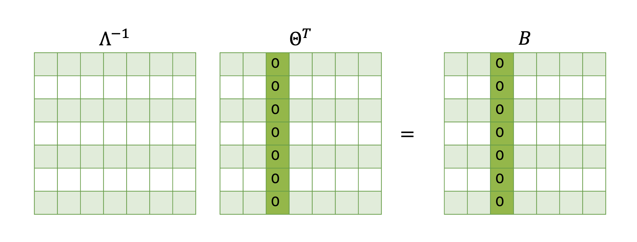
Figure 1: Demonstration of the use of group sparsity

While both the approaches, estimating $(\Theta,\Lambda)$ to get a group sparse $B$, and estimating $(B,\Lambda)$ to get a group sparse $\Theta$ are valid methods, the log-likelihood function of the GCRF is convex, while the one from the multivariate regression is not convex (Yuan and Zhang,, 2014). Thus, we formulate a method for the simultaneous sparse estimation of $(\Lambda,\Theta,B)$ using the GCRF framework. We induce the structural sparsity in our estimates by choosing appropriate priors.

3 Proposed adaptive Bayesian regularization framework

We propose a Bayesian regularization framework to sparsely estimate $(\Theta,\Lambda)$ for the GCRF model such that it leads to group-sparse estimates for $\Theta$ and $B$. In particular, we place appropriate priors on $\Theta$ and $\Lambda$ to induce the desired structural sparsity in the estimates. The prior likelihood is a product of the priors on $\Theta$ and $\Lambda$, $\Pi(\Theta,\Lambda)=\Pi(\Theta)\Pi(\Lambda).$ The negative posterior distribution $L(\Theta,\Lambda)$ corresponding to the prior distribution is then minimized to find the MAP (maximum a posteriori) estimators for $\Theta$ and $\Lambda$:

$$\min_{\Theta,\Lambda\succeq 0}L(\Theta,\Lambda).$$

We propose two different approaches for estimating the regression coefficient matrix $B$ from our estimates of $(\Theta,\Lambda)$:

1. A natural approach is to use plug-in estimation in the equation $B=-\Lambda^{-1}\Theta^{T}$. However, when $p$ is large, the error from inverting $\Lambda$, a $p\times p$ matrix, accumulates.

2. An alternate approach involves dropping the completely irrelevant covariates, identified as $X_{i}$ if $\hat{\Theta}_{i.}=\textbf{0}$. Then the remaining covariates are used to train multiple regression models, with each model corresponding to a single response $Y_{i}$ regressed on the remaining $X$’s. This approach is better suited for scenarios with large $p$.

The advantages and disadvantages of using each of these estimates are detailed in our theoretical results in Section 4. We now provide a detailed explanation of each aspect of the prior formulation and estimation process for the optimal $(\Theta,\Lambda)$.

3.1 Prior formulation

For our prior set-up, we place a spike and slab LASSO (SSL) prior (Ročková,, 2018) on $\Lambda$ and a mixture of the SSL prior and only a spike prior on $\Theta$

$$\Pi(\Theta) =\prod_{i}\bigg{[}\rho\prod_{j}\bigg{(}\eta^{\Theta}LP(\Theta_{ij},\nu_{1}^{\Theta})+(1-\eta^{\Theta})LP(\Theta_{ij},\nu_{0}^{\Theta})\bigg{)}$$

$$\quad\quad\quad\quad\quad+(1-\rho)\prod_{j}LP(\Theta_{ij},\nu_{0}^{\Theta})\bigg{]},$$

$$\Pi(\Lambda) =\prod_{i<j}\bigg{(}\eta^{\Lambda}LP(\Lambda_{ij},\nu_{1}^{\Lambda})+(1-\eta^{\Lambda})LP(\Lambda_{ij},\nu_{0}^{\Lambda})\bigg{)}.$$ (3)

To understand the motivation behind the choice of the priors, we present an alternative hierarchical form of our prior setup, which will also be used to formulate our EM algorithm. Consider the row-level binary indicator $r_{i}^{\Theta}$ and the element-level binary indicators $r_{ij}^{\Theta}$ and $r_{ij}^{\Lambda}$. These indicators serve as latent variables, which provide an alternative way of specifying our priors. The superscript ($\Theta$ or $\Lambda$) denotes the specific parameter to which each indicator corresponds. $r_{i}^{\Theta}$ indicates whether a complete row in $\Theta$ is zero ($r_{i}^{\Theta}=0$) or not ($r_{i}^{\Theta}=1$), thus indicating the row-wise sparsity. $r_{ij}^{\Theta}$ and $r_{ij}^{\Lambda}$ indicate the sparsity of the corresponding entries $\Theta_{ij}$’s and $\Lambda_{ij}$’s. The row-level binary indicator ($r_{i}^{\Theta}$) induces a hierarchical sparsity structure on $\Theta$ since $r_{ij}^{\Theta}=0$ when $r_{i}^{\Theta}=0$, but can take both $0$ and $1$ as values when $r_{i}^{\Theta}=1$.

We use spike and slab LASSO (SSL) priors, which have a well-established history within the Bayesian variable selection domain (Bai et al.,, 2020), to achieve the desired sparsity patterns. The “spike” part of the prior induces values to be close to zero, while the “slab” part accounts for the possibility that some elements can take non-zero values. In particular, given the binary indicators $r_{i}^{\Theta}$, $r_{ij}^{\Theta}$ and $r_{ij}^{\Lambda}$, we place a spike prior when the indicator $r_{.}=0$ and a slab prior when $r_{.}=1$. The diagonal entries of $\Lambda$ are generated from a uniform distribution. Since this leads to the corresponding prior likelihood for the diagonal entries to be independent of the parameters, they do not play a role in the posterior likelihood function, and thus, we avoid the diagonal entries in our notation. A similar hierarchical Bayesian framework has been applied to simultaneously estimate multiple graphical models in Yang et al., (2021). Our prior specification is graphically represented for ease of understanding in Figure 2 and can be summarized as follows:

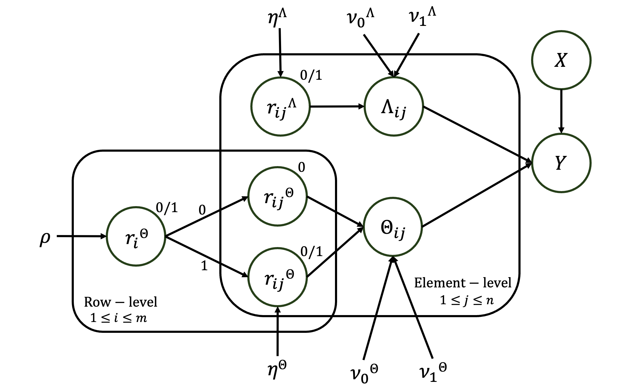
Figure 2: A graphical representation of our prior setup.

For $$\Theta \quad r_{i}^{\Theta}\sim Bern(\rho);\quad r_{ij}^{\Theta}|r_{i}^{\Theta}=1\sim Bern(\eta^{\Theta});\quad r_{ij}^{\Theta}|r_{i}^{\Theta}=0\sim\delta_{0}(r_{ij}^{\Theta});$$:

$$\quad\quad\quad\Theta_{ij}|r_{ij}^{\Theta}=1\sim LP(\Theta_{ij},\nu_{1}^{\Theta});\quad\Theta_{ij}|r_{ij}^{\Theta}=0\sim LP(\Theta_{ij},\nu_{0}^{\Theta}),$$

For $$\Lambda \quad r_{ij}^{\Lambda}\sim Bern(\eta^{\Lambda});\quad\Lambda_{ij}|r_{ij}^{\Lambda}=1\sim LP(\Lambda_{ij},\nu_{1}^{\Lambda});$$:

$$\quad\quad\quad\Lambda_{ij}|r_{ij}^{\Lambda}=0\sim LP(\Lambda_{ij},\nu_{0}^{\Lambda}),$$ (4)

where $LP(\Phi,\nu)=\frac{1}{2\nu}\exp\left\{-\frac{|\Phi|}{\nu}\right\}$. Using this formulation, we get estimates of $\Theta$ and $\Lambda$ by optimizing the posterior log-likelihood.

3.2 Adaptive regularization and MAP estimation of $(\Theta,\Lambda)$

To get estimates for $(\Theta,\Lambda)$, we use the maximum a posteriori (MAP) estimator, which leads to a penalized likelihood optimization problem with an adaptive penalty. The adaptive nature of the penalty function helps reduce bias in the estimates. Due to the GCRF model (1), given a random sample of $n$ observations, $(X_{i},Y_{i})_{i=1}^{n}$, our corresponding log-likelihood function is

$$l(\Theta,\Lambda)=\frac{n}{2}\bigg{(}\log\det(\Lambda)-tr(S_{yy}\Lambda+2S_{xy}^{T}\Theta+\Lambda^{-1}\Theta^{T}S_{XX}\Theta)\bigg{)},$$ (5)

where $S_{yy}=\frac{1}{n}\sum_{i=1}^{n}Y_{i}Y_{i}^{T}$, $S_{xy}=\frac{1}{n}\sum_{i=1}^{n}X_{i}Y_{i}^{T}$ and $S_{xx}=\frac{1}{n}\sum_{i=1}^{n}X_{i}X_{i}^{T}$. Additionally, using the prior distribution functions defined in (3.1), we get the negative log-posterior $L(\Theta,\Lambda)$:

$$L(\Theta,\Lambda)=-l(\Theta,\Lambda)+\sum_{i}Pen_{\text{MSS}}(\Theta_{i})+\sum_{i<j}Pen_{\text{SS}}(\Lambda_{ij})+const,$$ (6)

where $\sum_{i}Pen_{\text{MSS}}(\Theta_{i}):=-\log\Pi(\Theta)$ and $\sum_{i<j}Pen_{\text{SS}}(\Lambda_{ij}):=-\log\Pi(\Lambda)$. With the negative log-posterior defined as above, finding the MAP estimator for $(\Theta,\Lambda)$ is equivalent to solving the optimization problem:

$$\operatorname*{arg\,min}_{\Theta,\Lambda\succeq 0,\|\Lambda\|_{2}<R}L(\Theta,\Lambda).$$ (7)

Here, we impose two key conditions: $\Lambda\succeq 0$ and $|\Lambda|_{2}<R$, where the latter represents a bounded second norm of $\Lambda$. Such constraints have been previously used in Gan et al., (2022). The first condition is essential as it ensures that $\Lambda$ remains positive definite, a requirement stemming from its role as the inverse of a covariance matrix (2). While the second constraint introduces some limitations to the high-dimensional parameter space, it is important to note that the upper bound $R$ is flexible and can vary depending on the values of $n$, $p$, and $q$. Consequently, it can be set to relatively large values, making this restriction less severe and adaptable to the specific characteristics of the problem at hand.

The minimizer of (7) has a natural interpretation as the penalized likelihood estimator using the penalty functions which are induced by the Bayesian SSL priors. We will now introduce a proposition that demonstrates the concavity and the adaptive nature of the penalty functions $Pen_{\text{MSS}}(\Theta_{i})$ and $Pen_{\text{SS}}(\Lambda_{ij})$ in (6). These findings extend the results regarding the derivatives of the spike and slab prior outlined in Lemma 1 of Ročková and George, (2018). Before we delve into the statement of the proposition, we introduce some terms. Let $\eta_{1}(\phi)$ and $\eta_{2}(\phi)$ be defined as follows:

$$\eta_{1}(\phi) =\frac{\eta^{\phi}LP\left(\phi,\nu_{1}\right)}{\eta^{\phi}LP\left(\eta^{\phi},\nu_{1}^{\phi}\right)+(1-\eta^{\phi})LP\left(\eta^{\phi},\nu_{0}^{\phi}\right)},$$

$$\eta_{2}(\phi) =\frac{\rho S_{1}(\phi)}{\rho S_{1}(\phi)+(1-\rho)S_{2}(\phi)},$$ (8)

where $S_{1}(\phi)=\prod_{j}\left(\eta^{\phi}LP(\phi_{j},\nu_{1}^{\phi})+(1-\eta^{\phi})LP(\phi_{j},\nu_{0}^{\phi})\right)$ and $S_{2}(\phi)=\prod_{j}LP(\phi_{j},\nu_{0}^{\phi})$. From the definition of the terms $\eta_{1}(.)$ and $\eta_{2}(.)$, it is worth noting that $\eta_{1}(.)$ gives the probability of an individual element belonging to the “non-slab” component (or the “spike” component) and $\eta_{2}(.)$ gives the probability of a complete row belonging to the “non-slab” component. The proposition is as follows:

Proposition 1.

With $\eta_{1}(\phi)$ and $\eta_{2}(\phi)$ as defined as in (3.2), the following holds:

• $Pen_{\text{SS}}(\Lambda_{ij})$ and $Pen_{\text{MSS}}(\Theta_{i})$ are concave functions and

• The first derivatives of $Pen_{\text{SS}}(\Lambda_{ij})$ and $Pen_{\text{MSS}}(\Theta_{i})$ are given by

  $$\frac{\partial}{\partial|\Lambda_{ij}|}Pen_{\text{SS}}(\Lambda_{ij})=\frac{\eta_{1}(\Lambda_{ij})}{\nu_{1}^{\Lambda}}+\frac{1-\eta_{1}(\Lambda_{ij})}{\nu_{0}^{\Lambda}},$$

  $$\frac{\partial}{\partial|\Theta_{ij}|}Pen_{\text{MSS}}(\Theta_{i})=\frac{\eta_{1}(\Theta_{ij})\eta_{2}(\Theta_{i})}{\nu_{1}^{\Theta}}+\frac{1-\eta_{1}(\Theta_{ij})\eta_{2}(\Theta_{i})}{\nu_{0}^{\Theta}}.$$

According to Fan and Li, (2001), an effective adaptive penalty function should possess the properties of unbiasedness and sparsity. From the proposition above, we observe that the derivative of our penalty functions can be interpreted as a weighted mean of a small penalty $1/\nu_{1}$ and a large penalty $1/\nu_{0}$ with the weights $\eta$ and $1-\eta$ respectively representing the conditional probabilities of belonging to the “spike” and “slab” components. Consequently, when the parameter ($\Theta$ or $\Lambda$) is large, the derivative of the penalty is small. This means that significant fluctuations in the parameter values have little impact on the level of penalization. Essentially, the existence of the small penalty term reduces the bias due to over-shrinkage. Conversely, when the parameter is small, the derivative of the penalty functions is large. This effectively leads to a thresholding rule, driving certain entries towards zero and eliminating noisy contributions.

3.3 Optimization via an EM algorithm

Algorithm 1 EM Algorithm for Optimization of Posterior Log Likelihood

$X,Y$

Optimized parameters $\Theta,\Lambda,B$

Initialize: $\Theta\leftarrow 0$, $\Lambda\leftarrow I$

while (not converged) do

     (E-Step:)

     Calculate $p^{\Theta}={\rm I\kern-3.00003ptE}\left(r^{\Theta}\right),\;p^{\Lambda}={\rm I\kern-3.00003ptE}\left(r^{\Lambda}\right)$

     (M-Step:)

     while (not converged) do

         Determine active sets $A_{\Theta},A_{\Lambda}$, using (10)

         Compute the Newton updates $\Delta_{\Theta},\Delta_{\Lambda}$ for the elements in the active sets by optimizing (9).

         Set $\Delta_{\Theta},\Delta_{\Lambda}$ = 0 for elements in the non-active sets ($A_{\Theta}^{C},A_{\Lambda}^{C}$)

         Determine step size $\alpha$ using backtracking line search

         Update $\Theta\leftarrow\Theta+\alpha\Delta_{\Theta},\;\;\Lambda\leftarrow\Lambda+\alpha\Delta_{\Lambda}$

     end while

end while

if $p$ is small then

     Compute $B=-\Lambda^{-1}\Theta^{T}$

else

     Drop covariate $X_{i}$ if $\Theta_{i.}=\textbf{0}$. Create a new design matrix $\tilde{X}$ with only the selected covariates.

     Compute every row of $B$ as $B_{j.}^{T}=\hat{\beta}^{OLS}_{j}$, where $\hat{\beta}^{OLS}_{j}$ is the ordinary least square estimator for the model

$$M_{j}:Y_{.j}=\tilde{X}\beta_{j}+\varepsilon_{j};\quad j=\{1,2,\dots,p\}$$

end if

To solve the penalized optimization problem defined in (7), we develop an efficient EM algorithm (Algorithm 1), which uses a cyclic coordinate descent method. The proposed EM algorithm for the GCRF model is motivated by similar past works (Ročková and George,, 2014; Wytock and Kolter,, 2013; Ročková and George,, 2016; Gan et al.,, 2022). First, we reparametrize the objective function (7) using the latent variables $r^{\Theta}_{ij}$ and $r^{\Lambda}_{ij}$ and the alternative prior setup defined in 3.1. In the E-step of our algorithm, at every iteration of the cyclic coordinate descent, we find estimates $p^{\Theta}_{ij}$ and $p^{\Lambda}_{ij}$ for $r^{\Theta}_{ij}$ and $r^{\Lambda}_{ij}$ respectively. The expectation of the reparametrized objective function is then computed to derive $Q(\Phi|\Phi^{(t)})$ $(\Phi=(\Theta,\Lambda))$ which is minimized in the M-Step:

$$Q(\Phi|\Phi^{(t)})=-l(\Phi)+\sum_{i<j}\left(\frac{p_{ij}^{\Phi(t)}}{\nu_{1}^{\Phi}}+\frac{1-p_{ij}^{\Phi(t)}}{\nu_{0}^{\Phi}}\right)|\Phi_{ij}|+const.$$ (9)

The fundamental concept underlying our M-step involves an iterative process where we sequentially construct a second-order approximation to the M-step objective function $Q(\Phi|\Phi^{(t)})$. Subsequently, the cyclic coordinate descent algorithm transforms the problem into a simplified Lasso form. Solving this Lasso problem yields the Newton update step. Due to the sparse nature of our estimated parameters, we make our algorithm faster by only updating the elements in the active set during our coordinate descent instead of updating all the elements. We define the active set for both $\Theta$ and $\Lambda$ as follows:

$$\left|\big{(}\nabla_{\Phi}l(\Theta,\Lambda)\big{)}_{ij}\right|>\left|\big{(}\nabla_{\Phi}Pen(\Phi)\big{)}_{ij}\right|\quad\text{ or }\quad\Phi_{ij}\neq 0,$$ (10)

where $\Phi$ = ($\Theta$,$\Lambda$), $Pen(\Theta)=\sum_{i}Pen_{\text{MSS}}(\Theta_{i})$ and $Pen(\Lambda)=\sum_{i<j}Pen_{\text{SS}}(\Lambda_{ij})$. Using the estimates of $\Lambda$ and $\Theta$ obtained, $B$ is estimated using plug-in when $p$ is small or by training multiple linear regression models when p is large. Further details on the EM algorithm can be found in the Supplementary Materials.

3.4 Structure Recovery based on Marginal Inclusion Probabilities

An important aspect of our method is its ability to detect the sparsity patterns and recover the structure of the matrices. We quantify the uncertainty of these sparsity patterns by means of the marginal inclusion probabilities of the parameters. To achieve this, we use the binary indicators $r_{ij}^{\Theta}$ and $r_{ij}^{\Lambda}$, as defined in Section 3.1, which serve the purpose of indicating whether the elements within the corresponding matrices $(\Theta,\Lambda)$ are nonzero or not. The marginal inclusion probability for an element of $\Lambda$ is given by the probability of the corresponding $r_{ij}^{\Lambda}=1$ which can be computed to be

$$P(r_{ij}^{\Lambda}=1|\Lambda)=\eta_{1}(\Lambda_{ij}).$$

Similarly, the marginal inclusion probability for an element of $\Theta$ is given by the probability of the corresponding $r_{ij}^{\Theta}=1$ which can be computed to be

$$P(r_{ij}^{\Theta}=1|\Theta)=P(r_{i}^{\Theta}=1|\Theta_{i})P(r_{ij}^{\Theta}=1|r_{i}^{\Theta}=1,\Theta_{ij})=\eta_{2}(\Theta_{i})\eta_{1}(\Theta_{ij}),$$

with $\eta_{1}(.)$ and $\eta_{2}(.)$ as defined in 3.2. From the above equation, we can understand how information is shared across rows due to the induced row-wise sparsity. The marginal inclusion probability for $\Theta_{ij}$ is factored into two parts. The first part given by $P(r_{i}^{\Theta}=1|\Theta_{i})=\eta_{2}(\Theta_{i})$ gives information regarding the row-wise inclusion probability and the second part $P(r_{ij}^{\Theta}=1|r_{i}^{\Theta}=1,\Theta_{ij})=\eta_{1}(\Theta_{ij})$ gives information regarding the within-row inclusion probability. Thus, the product of the two considers both the row-wise and individual-level sparsity patterns for $\Theta$ while performing sparse structure recovery. Thus, given the MAP estimator for $(\Theta,\Lambda)$ we get from (7), we can estimate the sparsity pattern by thresholding the posterior inclusion probabilities by some $t\in[0,1]$ as follows:

$$r_{ij}^{\Lambda}=1\iff\eta_{1}(\Lambda_{ij})>t;\quad r_{ij}^{\Theta}=1\iff\eta_{1}(\Theta_{ij})\eta_{2}(\Theta_{i})>t.$$

This approach facilitates the identification of non-zero elements, aiding in recovering the structural sparsity for the matrices involved in our model.

4 Theoretical Results

In this Section, we provide theoretical results to support the effectiveness of our proposed method in recovering the structural sparsity of the parameters and achieving accurate variable selection. Additionally, we offer theoretical guarantees on the convergence of our estimates. Detailed proof of these results can be found in the Supplementary Materials. We begin by defining the notation used in the main results.

Notation:

To conduct the theoretical studies, we assume that our data $Y$ has been generated based on a fixed set of true parameters $(\Theta^{0},\Lambda^{0})$ and consider the true data-generating distribution to be sub-Gaussian with the random covariate vector $X$ having covariance $\Sigma^{0}_{xx}$. This is a frequentist data generation mechanism that is quite common in literature (Ishwaran and Rao,, 2005; Castillo et al.,, 2015; Narisetty and He,, 2014; Gan et al.,, 2019, 2022). We define the High Posterior Density (HPD) region:

$$HPD =\{(\Theta,\Lambda):\Pi(\Theta,\Lambda|Data)\geq\Pi(\Theta^{0},\Lambda^{0}|Data)\}$$

$$=\{(\Theta,\Lambda):L(\Theta,\Lambda)\leq L(\Theta^{0},\Lambda^{0})\},$$

where $L(\Theta,\Lambda)$ is the negative log posterior defined in (7). Thus, the HPD region contains all the parameter values with a posterior probability as much as the true value given the data. Let the signal set for $\Lambda$: $S^{\Lambda}=\{(i,j):\Lambda_{ij}^{0}\neq 0\}$ denote the set of element-wise signals in $\Lambda$, and signal sets for $\Theta$: $S_{row}^{\Theta}=\{(i,j):\Theta_{i.}^{0}\neq\underaccent{\tilde}{0}\}$ denote the row-wise signals and $S^{\Theta}=\{(i,j):\Theta_{ij}^{0}\neq 0\}$ denote the element-wise signals in $\Theta$. This leads us to define the joint sparsity sets $S^{0}_{row}:=S_{row}^{\Theta}\bigcup S^{\Lambda}$ and $S^{0}:=S^{\Theta}\bigcup S^{\Lambda}$. Additionally, let $\tilde{q}$ denote the number of relevant variables in the data: $\tilde{q}=card(\{i:\Theta^{0}_{i.}\neq 0\})$. For a matrix $\Phi$, we define $\lambda_{max}(\Phi),\lambda_{min}(\Phi)$ to be the largest and smallest eigenvalues of a matrix $\Phi$. We also define for $\Phi$ the Frobenius norm $\|\Phi\|_{F}:=\sqrt{\sum_{i}\sum_{j}|\Phi_{ij}|^{2}}$, the elementwise max norm $\|\Phi\|_{\infty}:=\max_{i,j}\Phi_{ij}$ and the absolute row sum matrix norm ${\left|\kern-1.07639pt\left|\kern-1.07639pt\left|\Phi\right|\kern-1.07639pt\right|\kern-1.07639pt\right|}_{\infty}:=\max_{i}\sum_{j}|\Phi_{ij}|$. Finally, we define the following constants

$$c_{H}=\frac{n}{2}{\left|\kern-1.07639pt\left|\kern-1.07639pt\left|H^{-1}_{S^{0}S^{0}}\right|\kern-1.07639pt\right|\kern-1.07639pt\right|}_{\infty},\quad c_{\Theta^{0}}={\left|\kern-1.07639pt\left|\kern-1.07639pt\left|\Theta^{0^{T}}\right|\kern-1.07639pt\right|\kern-1.07639pt\right|}_{\infty},\quad c_{\Lambda^{0}}={\left|\kern-1.07639pt\left|\kern-1.07639pt\left|(\Lambda^{0})^{-1}\right|\kern-1.07639pt\right|\kern-1.07639pt\right|}_{\infty},$$

where $H$ is the Hessian matrix $\nabla^{2}l(\Theta,\Lambda)$ and $H^{-1}_{S^{0}S^{0}}$ is the submatrix of $H^{-1}$ with the rows and columns indexed by $S_{0}$.

In addition to the notation above, we assume $\nu_{0}^{\Theta}=\nu_{0}^{\Lambda}$, $\nu_{1}^{\Theta}=\nu_{1}^{\Lambda}$, and $\eta^{\Theta}=\eta^{\Lambda}$ referring to them as $\nu_{1}$, $\nu_{0}$, and $\eta$ for simplicity. The conditions required for the terms corresponding to $\Lambda$ and $\Theta$ are nearly identical, and we will specify any differences when they arise. Our analysis also accommodates the growth of the quantities $(\nu_{0},\nu_{1},R)$, as well as model sizes $p,q$, and $|S^{0}_{row}|$, with the sample size $n$. However, for the sake of convenience, we omit the dependence on $n$ in our notation.

4.1 Preliminary results on the likelihood function

Before presenting our theoretical findings, we outline the key assumptions and properties of our likelihood function necessary for our theoretical results. These assumptions are not uncommon in the Gaussian Conditional Random Fields literature, with similar assumptions being considered in Yuan and Zhang, (2014) and Gan et al., (2022).

Assumptions: Assume that

• $X$ satisfies the following $s_{0}$-sparse restricted isometry property condition:

  $$\begin{cases}\inf\left(\frac{u^{T}S_{xx}u}{u^{T}\Sigma^{0}_{xx}u}:\;u\neq 0,\|u\|_{0}\leq s_{0}\right)\geq 0.5,\\ \sup\left(\frac{u^{T}S_{xx}u}{u^{T}\Sigma^{0}_{xx}u}:\;u\neq 0,\|u\|_{0}\leq s_{0}\right)\leq 1.5,\\ \frac{\lambda_{max}[(\Theta^{0})^{T}S_{xx}\Theta^{0}]}{\lambda_{max}[(\Theta^{0})^{T}\Sigma^{0}_{xx}\Theta^{0}]}\leq 1.4.\end{cases}$$

  with $s_{0}=|S^{0}_{row}|+\lceil 4(\rho_{2}/\rho_{1})\alpha^{2}|S^{0}_{row}|\rceil$, where $\rho_{1}=0.5\min(\lambda_{max}(\Lambda^{0})^{-1},\lambda_{min}(\Sigma^{0}_{xx}))$ and $\rho_{2}=1.5\lambda_{max}(\Sigma^{0}_{xx})$

• The sample size $n$ satisfies: $n>(p+s_{0})\log(p+q)/\varepsilon_{0}$ where $\varepsilon_{0}$ is a constant between $(0,1)$.

Candes and Tao, (2007) shows that in our setting of a sub-Gaussian $X$, with the corresponding $\Sigma_{xx}^{0}$ having eigenvalues that meet specific regularity conditions, assumption (a) holds with a high probability when assumption (b) is satisfied. Thus, the assumptions are not very restrictive.

Under the assumptions stated above, we can establish three important properties of the likelihood function, which are crucial for proving our theoretical results. While these properties have been established in prior works, we include them here for completeness and to keep our paper self-contained. The first property is that the derivative of the likelihood function is bounded. Specifically, as a direct consequence of Proposition 4 in Yuan and Zhang, (2014) we have $\|\nabla l(\Theta^{0},\Lambda^{0})\|_{\infty}\leq K\sqrt{\log(10(p+q)^{2}/\varepsilon_{0})/n}$ with probability $1-\varepsilon_{0}$, where $\varepsilon_{0}$ is any constant in $(0,1)$ and $K$ is a constant that depends on $\Theta^{0},\Lambda^{0}$ and $\Sigma^{0}_{xx}$.

Moreover, our likelihood function is strongly convex in the HPD region, a result supported by the following properties. Let the local restricted strong convexity (LRSC) constant, a quantity that measures the local curvature of $l(\Phi)$ at $\Phi^{0}$, be defined as:

$$\beta(\Phi^{0};r,\alpha)=\inf\bigg{\{}\left\langle\frac{\nabla l(\Phi^{0})-\nabla l(\Phi^{0}+\Delta),\Delta}{\|\Delta\|^{2}_{2}}\right\rangle;\quad\|\Delta\|_{2}\leq r,\|\Delta_{(S^{0}_{row})^{C}}\|_{1}\leq\alpha\|\Delta_{S^{0}_{row}}\|_{1}\bigg{\}}.$$

and let

$$r_{0} =min[0.5\lambda_{min}(\Lambda^{0}),0.13\sqrt{\lambda_{max}[(\Theta^{0})^{T}\Sigma^{0}_{xx}\Theta^{0}]/\rho_{2}}],$$

$$\beta_{0} =\left\{\frac{\rho_{1}}{40\lambda_{max}(\Lambda^{0})}\cdot min\left[1,\frac{\lambda_{min}(3\Lambda^{0})}{16\lambda_{max}[(\Theta^{0})^{T}\Sigma^{0}_{xx}\Theta^{0}]}\right]\right\}.$$

Then, under the assumptions stated above, we have the LRSC constant $\beta(\Phi^{0};r;\alpha)\geq n\beta_{0}$ for $r\leq r_{0}$. This property follows from Proposition 3 from Yuan and Zhang, (2014) and Lemma 2 in Gan et al., (2022), and gives a bound for the LRSC constant in the cone $\|\Delta_{(S^{0}_{row})^{C}}\|_{1}\leq\alpha\|\Delta_{S^{0}_{row}}\|_{1}$ showing that the likelihood function is strongly convex within this cone. Finally, using arguments similar to Lemma 3 in Gan et al., (2022) it can be shown that if $1/\nu_{1}>2\|l(\Theta^{0},\Lambda^{0})\|_{\infty}$, then for any $(\Theta,\Lambda)=(\Theta^{0},\Lambda^{0})+\Delta$ so that $(\Theta,\Lambda)\in HPD$, we have

$$\|\Delta_{(S^{0}_{row})^{C}}\|_{1}\leq\alpha\|\Delta_{S^{0}_{row}}\|_{1},$$ (11)

where $\alpha=1+2\nu_{1}/\nu_{0}.$ This confirms that all the points in the HPD belong to the cone (11), thus establishing the strong convexity of the likelihood function in the HPD region.

4.2 Convergence and sparse structure recovery of the precision matrices $(\Theta,\Lambda)$

4.2.1 Rate of convergence for all the points in the HPD

In our first theorem, we demonstrate that every $\Theta$ and $\Lambda$ within the HPD region closely approximates the true parameter with an optimal level of statistical precision in the Frobenius norm.

Theorem 1.

Let the following conditions hold along with the assumptions stated above:

1. The hyperparameters $\nu_{1}$ and $\nu_{0}$ follow

   $$\frac{1}{n\nu_{0}}\in\mathcal{O}\left(\sqrt{\frac{\log(p+q)}{n}}\right),\frac{1}{n\nu_{1}}\in\mathcal{O}\left(\sqrt{\frac{\log(p+q)}{n}}\right)$$

   and

   $$1/\nu_{1}>2\|\nabla l(\Theta^{0},\Lambda^{0})\|_{\infty};$$

2. $R<\frac{2\lambda_{max}(\Lambda^{0})\sqrt{r_{0}}}{\epsilon_{n}}$, where R is the matrix norm bound for $\Lambda$ and $\epsilon_{n}$ is as defined below;

then for any $(\Theta,\Lambda)\in HPD$, with probability at least $1-\epsilon_{0}$, we have

$$\|(\Theta,\Lambda)-(\Theta^{0},\Lambda^{0})\|_{F}\leq\epsilon_{n}:=\frac{C}{\beta_{0}}\sqrt{\frac{|S^{0}_{row}|\log(p+q)}{n}}\rightarrow 0,$$

where $\epsilon_{0}$ is a constant in $(0,1)$.

The above theorem shares notable similarities in its conditions with Theorem 1 in Gan et al., (2022). Our results also align with Gan et al., (2022) in terms of the convergence rates for $(\Theta,\Lambda)$ that is, if the sample size follows assumption (b), then $\epsilon_{n}$ goes to zero. A similar result has been demonstrated for the Lasso penalty function by Yuan and Zhang, (2014) concerning the global optimum for $(\Theta,\Lambda)$. Turning our attention to methods that focus on the estimation of $(B,\Lambda)$, Yin and Li, (2011) and Cai et al., (2013) also provide comparable convergence rates for the global optimum for $\Lambda$. However, our results are advantageous over the latter methods since we show our convergence rates for all points in the HPD, not only for the global optimum.

4.2.2 Faster convergence rates and sparsistency for a local optimum

Our following theorem presents stronger estimation and selection accuracy results, specifically for at least one locally stationary point within the HPD. Additionally, we demonstrate that this optimal stationary point achieves sparsistency, meaning that the parameter estimates are correctly set to zero in places where the true parameter is indeed zero.

Theorem 2.

Let the assumptions stated above hold. Then with probability $1-\epsilon_{0}$ there exists a stationary point $(\hat{\Theta},\hat{\Lambda})\in HPD$ such that

$$\hat{\Theta}_{(S^{\Theta})^{C}}=\hat{\Lambda}_{(S^{\Lambda})^{C}}=0,$$

and

$$\max\left\{\|\hat{\Theta}-\Theta^{0}\|_{\infty},\|\hat{\Lambda}-\Lambda^{0}\|_{\infty}\right\}\leq r_{n}:=4C_{3}c_{H}\sqrt{\frac{\log(p+q)}{n}},$$

where $\epsilon_{0}$ is a constant in $(0,1)$, if the following conditions hold:

1. The hyper-parameters $\nu_{1},\nu_{0}$ and $\rho$ follow condition (i) stated in Theorem 1 along with the following:

   $$\left(\frac{\nu_{1}}{\nu_{0}}\right)^{p+2}\frac{(1-\rho)}{\rho(\eta)^{p}}\leq\epsilon_{1}(p+q)^{\epsilon_{2}};\quad\left(\frac{\nu_{1}}{\nu_{0}}\right)^{3}\frac{(1-\eta)}{\eta}\leq\epsilon_{1}(p+q)^{\epsilon_{2}};\quad\frac{1}{n\nu_{0}}>C_{4}\sqrt{\frac{\log(p+q)}{n}}$$

   where $\epsilon_{1},\epsilon_{2},C_{1},C_{3}$ and $C_{4}$ are positive constants with $C_{3}>C_{1}$, $C_{4}>C_{1}$ and $\epsilon_{2}=(C_{3}-C_{1})c_{H}(C_{4}-C_{1})$;

2. The minimum signal strength for $\Theta$ and $\Lambda$ are both greater than $r_{n}$ i.e. $\min\{\Theta^{0}_{min},\Lambda^{0}_{min}\}>r_{n}$;

3. $r_{n}<\min\bigg{\{}\frac{2C_{4}\sqrt{\log(p+q)/n}}{\left(1/2c_{H}+c_{H}\right)}\frac{(1-\eta)\nu_{0}}{(1-\eta)\nu_{0}+\eta\nu_{1}},\frac{1}{3dc_{\Lambda^{0}}},\frac{c_{\Theta^{0}}}{2d},\frac{1}{7416d^{2}c_{\Theta^{0}}^{2}c_{\Lambda^{0}}^{4}\rho_{2}}\bigg{\}}$ and $\beta_{0}>\frac{C_{1}^{2}\log(p+q)}{4(p+q)^{\epsilon_{2}}}$.

Remark 1: If we consider $\nu_{1}^{\Theta}\neq\nu_{1}^{\Lambda}$ and $\nu_{0}^{\Theta}\neq\nu_{0}^{\Lambda}$, then the first condition in condition (i) is only required for the parameters corresponding to $\Theta$.

Remark 2: The estimators for $\Theta,\Lambda$ and $B$ obtained in Theorem 2 are unique if there exists an $m>0$, such that $\beta_{0}\geq\left(\frac{1}{4}+\frac{p}{8}\right)\frac{C_{1}^{2}\log(p+q)}{(p+q)^{\epsilon_{2}}}+\frac{m}{2n}$, where $\epsilon_{2}=(C_{3}-C_{1})c_{H}(C_{4}-C_{1})$ with $C_{1},C_{3},C_{4}$ as defined in Theorem 2.

In the above theorem, condition (i) enables our estimates to achieve adaptive shrinkage by regulating the rate of $1/\nu_{0}$ and $1/\nu_{1}$, as explained in Section 3.2. Furthermore, contrasting condition (i) in Theorem 2 with that in Theorem 1, we observe that Theorem 2 needs $\eta$ to fall strictly between $0$ and $1$, a requirement absent in Theorem 1. Hence, the Lasso penalty, being a specific case of the spike and slab penalty where $\eta$ is constrained to be either $0$ or $1$, fails to meet the conditions. Condition (ii) is the beta-min condition, commonly used in sparse parameter estimation, requiring the minimum signal strength to be sufficiently large in the true model to help identify the relevant parameters. A construction-based proof for Theorem 2 motivated by similar proofs in Ravikumar et al., (2011); Wytock and Kolter, (2013); Loh and Wainwright, (2013); Gan et al., (2019, 2022) is provided in the Supplementary materials.

The convergence rates for $(\Theta,\Lambda)$ in Theorem 2 are comparable to the results in Wytock and Kolter, (2013) and Gan et al., (2022), though the former method requires the mutual incoherence condition, which is more restrictive than our conditions (see Section 3.3 of Gan et al., (2022) for a comprehensive discussion). While our results for $(\Theta,\Lambda)$ mirror the results from Gan et al., (2022), our group-sparse setup has the additional advantage of providing column-sparse estimates for $B$, which we elaborate on in Section 4.3. Additionally, Yin and Li, (2011) and Cai et al., (2013) provide similar results for their estimates of $\Lambda$.

4.3 Convergence and structure recovery for the regression coefficient matrix $B$

In Section 3, we introduce two different approaches for estimating the regression coefficient matrix from our estimates of $(\Theta,\Lambda)$. We now present structure recovery and convergence results for both these estimates. Given that our framework does not directly optimize for the best estimate of $B$, achieving perfect convergence rates without any trade-offs is quite challenging. Consequently, we also provide a discussion on the pros and cons of using each of the estimates in terms of their convergence rates.

Results for the plug-in estimator:

The plug-in estimator involves estimating the regression coefficient matrix as $\hat{B}=-\hat{\Lambda}^{-1}\hat{\Theta}^{T}$ where $(\hat{\Theta},\hat{\Lambda})$ are the estimates for $(\Theta,\Lambda)$. Recall, Theorem 2 proves that the optimal stationary point for $\Theta$ achieves row sparsistency i.e. $\hat{\Theta}_{S^{\Theta}_{row}}\neq 0$ and $\hat{\Theta}_{(S^{\Theta}_{row})^{C}}=0$. As a direct consequence of Theorem 2, we obtain column sparsistency for the plug-in estimate $\hat{B}$. This result is presented in Corollary 1. Proving this corollary is straightforward using the insights on combined group sparsity of $\Theta$ and $B$ provided in Section 2. Note that column sparsistency implies that the totally irrelevant covariates in the true model are assigned entirely zero columns in the estimated regression coefficient matrix. Thus, this result showcases that our method can achieve effective variable selection.

Corollary 1.

Let $(\hat{\Theta},\hat{\Lambda})$ be as defined in Theorem 2. If the conditions stated in Theorem 2 hold, the plug-in estimate $\hat{B}:=-\hat{\Lambda}^{-1}\hat{\Theta}^{T}$ has the following property, with probability $1-\epsilon_{0}$:

$$\hat{B}_{(S^{B}_{col})^{C}}=0,$$

where $S_{col}^{B}$ is the transpose of $S_{row}^{\Theta}$ denoting the set of column-wise signals in $B^{0}$ and $\epsilon_{0}$ is a constant in $(0,1)$.

In fact, the above result trivially generalizes for any $\hat{B}$ estimated using $\hat{B}=\Phi\hat{\Theta}^{T}$, where $\Phi$ is a $p\times p$ matrix and $\hat{\Theta}$ is an estimate of $\Theta$ that achieves row sparsistency. In addition to the sparsity structure recovery, we also establish some convergence results for the plug-in estimate. However, this estimator requires the inversion of a $p\times p$ matrix, the error of which adds up as $p$ grows with $n$ to infinity. Thus, we present the convergence results for this estimator only under a fixed $p$ scenario.

Corollary 2.

Under a fixed $p$, for any $(\Theta,\Lambda)\in HPD$, if the conditions stated in Theorem 1 hold, the estimate $B:=-\Lambda^{-1}\Theta^{T}$ has

$$\|B-B^{0}\|_{F}\leq\frac{F_{\Lambda}\epsilon_{n}}{1-F_{\Lambda}\epsilon_{n}}(1+F_{\Lambda}F_{\Theta}),$$

with probability greater than $1-\epsilon_{0}$, where $\epsilon_{0}$ is a constant, $F_{\Lambda}:=\|(\Lambda^{0})^{-1}\|_{F}$ and $F_{\Theta}:=\|\Theta^{0}\|_{F}$.

In the above corollary, the Frobenius norm of $\Lambda^{-1}$ grows in the order $\sqrt{p}$ and the Frobenius norm of $\Theta^{0}=\mathcal{O}(|S^{\Theta}|)$. Since we consider a sparse setup, the number of signals present in $\Theta^{0}$, denoted by $|S^{\Theta}|$, is expected to be small compared to $n$. Therefore, in the fixed $p$ scenario, both $F_{\Lambda}$ and $F_{\Theta}$ are controlled, leading to the bound of the Frobenius norm of the difference between the estimate and the true parameter approaching zero. An advantage of this estimate is that our result encompasses all points within the high probability density (HPD) region, including the global optimum. This contrasts with other methods such as Cai et al., (2013), which focus solely on results for the optimum point. The limitation of this estimate is when $p$ grows with $n$, the bound is too loose, as $F_{\Lambda}$ is no longer controlled. It is worth mentioning here that while a theoretical convergence result cannot be established in this scenario, our simulations (in Section 5) indicate that the plug-in estimate performs well for reasonably large values of $p$. Alternatively, where the direct plug-in is not useful, our result for $\hat{\Theta}$ gives us another effective way of estimating $B$.

Results for estimating $B$ via multiple linear regression models:

In this approach, we estimate the regression coefficient matrix by excluding any $X_{i}$ for which the optimal $\hat{\Theta}$ from Theorem 2 yields $\hat{\Theta}_{i.}=\textbf{0}$. Due to the row sparsistency of $\hat{\Theta}$, we effectively drop variables corresponding to 0-columns in $B^{0}$, thus achieving perfect column-structure recovery for $B$. This is equivalent to the result for the plug-in estimate in Corollary 1.

Let $\tilde{X}_{n\times\tilde{q}}=(X_{1},X_{2},\dots,X_{\tilde{q}})$ represent the design matrix comprising the variables selected through this process. Note that we have exactly $\tilde{q}$ many variables remaining since we attain perfect variable selection. Subsequently, we estimate $\tilde{B}$ using $p$ linear regression models, where each model $M_{j}$ is defined as:

$$M_{j}:Y_{.j}=\tilde{X}\tilde{B}_{j.}^{T}+\varepsilon_{j};\quad j=\{1,2,\dots,p\}.$$

In particular, every row of $\tilde{B}$ (denoted as $\tilde{B}_{j.}$) is estimated using the ordinary least squares estimator for model $M_{j}$. The estimate for $B$ can then be obtained by appending $q-\tilde{q}$ many 0-columns to $\hat{\tilde{B}}$ corresponding to the irrelevant covariates. That is, $\hat{B}=\left[\hat{\tilde{B}}_{\tilde{q}\times p}:\textbf{0}_{(q-\tilde{q})\times p}\right]$. The following corollary gives the convergence rate for the estimated $B$.

Corollary 3.

If the conditions for Theorem 2 hold along with the condition $\lambda_{min}(\tilde{X})>0$, then with probability greater than $1-\mathcal{O}\{(p+q)^{-1}\}$, the estimate $\hat{B}$ using the above approach satisfies

$$\frac{1}{\sqrt{p}}\|\hat{B}-B^{0}\|_{F}\leq\frac{K}{\lambda_{min}(\tilde{X})}\sqrt{\frac{\tilde{q}+\log\left(p+q\right)}{n}},$$

where K is a constant.

The above corollary follows from standard results for ordinary least square estimators for regression coefficients (Rigollet,, 2015). Our estimation error for $B$ has the same rate as the bound described in Cai et al., (2013), even though our method does not explicitly optimize for an estimate of $B$. Additionally, while Cai et al., (2013) provides convergence results for $B$, they lack similar results for $\Theta$. Comparing the two estimation approaches for $B$, note that our results for the plug-in estimator require the conditions for Theorem 1 to hold, whereas the multiple linear regressions estimator requires the conditions for Theorem 2, which are stronger. Additionally, the results we provide here are solely for the optimal point and not all points in the HPD, unlike the plug-in estimator. Thus, when $p$ is reasonable, using the plug-in approach is preferable.

5 Experimental Results

In this Section, we first provide some simulation studies, followed by an analysis of a bike-share data set using our proposed method for Bayesian variable selection for graphical models (denoted by BVS.GM). In all the experimental studies, we estimate $B$ using the plug-in estimator, as it demonstrates good convergence results even when $p$ is reasonably large.

5.1 Simulation Studies

We conduct a comparative analysis of various methods against BVS.GM in terms of estimation and structure recovery. The methods under comparison include Graphical LASSO (or GLASSO), which was introduced in Friedman et al., (2008), CAPME, which was introduced in Cai et al., (2013), and Bayes CRF (or BCRF), which was introduced in Gan et al., (2022). For our simulation setup, we generate the covariate matrix X from a zero-mean multivariate normal distribution. We construct X with a sparse tri-diagonal Toeplitz precision matrix $\Omega_{xx}:=Toeplitz(0.3,1,0.3)$. This means that the diagonal of $\Omega_{xx}$ is set to 1, while the sub-diagonal and super-diagonal elements are set to 0.3. The true parameters of the conditional random field, denoted as $(\Theta^{0},\Lambda^{0})$, are generated with high sparsity as follows:

$\Lambda^{0}$: We create this matrix to contain a fixed number of non-zero elements ($s_{\Lambda^{0}}$) in the upper triangular off-diagonal section. The non-zero elements are generated from a uniform distribution. Since the matrix is symmetric, we generate values only for the upper-triangular off-diagonal part. To ensure that the matrix remains positive semi-definite, we set the diagonal elements to be 0.2 greater than the sum of the off-diagonal elements in their respective rows, i.e., $\Lambda^{0}_{ii}=\sum_{j\neq i}|\Lambda^{0}_{ij}|+0.2$.

$\Theta^{0}$: We design this matrix to have a $70\%$ percent of the rows entirely filled with zeros. The zero rows ensure that some covariates $X$ exist that do not impact the response. For the remaining rows, we generate the non-zero elements using two different methods. The first method involves sampling a fixed number of non-zero elements ($s_{\Theta^{0}}$) independently from a uniform distribution. Consequently, each non-zero element is treated as independent, with the maximum signal strength being the largest magnitude among the non-zero elements. In the second method, we use a randomized approach to determine the number of non-zero elements in each row, randomly sampled from $Unif(0.1*p,0.5*p)$. Then, these non-zero elements are generated from a uniform sphere with a constant norm. For example, consider a scenario with $p=10$ where the number of non-zero elements in a row is randomly determined to be 3. In this case, the non-zero elements are generated from a 3-dimensional uniform sphere with a fixed norm. Here, the fixed norm determines the signal strength, and the elements within a row are no longer treated as independent.

Finally, we generate the response variable $Y$ given $X$ using the covariate-adjusted graphical model, specifically, $Y\sim N(B^{0}X,(\Lambda^{0})^{-1})$, where $B^{0}=-(\Lambda^{0})^{-1}(\Theta^{0})^{T}$ represents the true regression coefficient matrix. In the case of lower-dimensional simulation scenarios, we consider seven distinct values for the number of observations, $N=(20,40,100,200,500,1000,10000)$. For the higher-dimensional simulation scenarios, we explore four options for $N=(100,500,1000,2000)$. The reported results are obtained as averages over $20$ replications for each specific value of N. The performance metrics we consider are:

• Estimation error: Using the Frobenius norm of the difference between the estimated parameter and the true parameter.

• Structure recovery: Using MCC (Matthews Correlation Coefficient) which is defined as

  $$MCC=\frac{(TP*TN)-(FP*FN)}{\sqrt{(TP+FP)(TP+FN)(TN+FP)(TN+FN)}}$$

  where TP denotes the true positives, TN denotes the true negatives, FP denotes the false positives and FN denotes the false negatives.

• Column recovery for B: Using MCC for the columns where $0$ denotes a column which is fully 0, and $1$ when the column contains any non-zero element.

We present the results for three simulation scenarios that we believe most effectively showcase the strengths of our method. Additionally, we have conducted numerous other simulations to assess the performance of our method in different setups, and these results are provided in the Supplementary Materials.

5.1.1 Set-up 1: Low signal strength, low dimensional setting with independent non-zero elements in Theta

In this setup, we consider the number of responses $p=10$, the number of covariates $q=50$, the number of non-zero elements in the non-zero rows of $\Theta^{0}$ ($s_{\Theta^{0}}$) = 10 and the number of non-zero elements in $\Lambda^{0}$ ($s_{\Lambda^{0}}$) = 5. This implies that $\Lambda^{0}$ has $10$ non-zero off-diagonal elements but since it is symmetric, only $5$ are uniquely estimated. $\Lambda^{0}$ also has p=10 non-zero diagonal elements. The non-zero elements for both $\Theta^{0}$ and $\Lambda^{0}$ are generated from $Unif\left([-0.2,-0.1]\cup[0.1,0.2]\right)$. Thus, the minimum signal strength is 0.2. The results for this setup are tabulated in tables 3,3 and 3.

5.1.2 Set-up 2: Low signal strength, low dimensional setting with non- zero elements dependent in Theta

In this setup, we once again consider $p=10$, $q=50$ and $s_{\Lambda^{0}}$ = 5. The non-zero elements for $\Lambda^{0}$ are still generated from $Unif\left([-0.2,-0.1]\cup[0.1,0.2]\right)$. But instead of the non-zero elements in $\Theta^{0}$ being independent, they are generated from a uniform sphere with norm = 0.5 using the method described above. Thus, these non-zero elements are dependent and have a low signal strength since the norm of a row is fixed to be less than $0.5$. The results for this setup are tabulated in tables 6,6 and 6.

5.1.3 Set-up 3: Low signal strength, high dimensional setting with non- zero elements dependent in Theta

This setup is a higher dimensional analogue of the previous setup. Here, we consider the number of responses $p=50$, the number of covariates $q=100$ and the number of non-zero elements in $\Lambda$ ($s_{\Lambda^{0}}$) = 100. The non-zero elements in $\Theta^{0}$ are generated from a uniform sphere with norm = 0.5. The results for this setup are tabulated in tables 9,9 and 9.

5.1.4 Discussion on the simulation results

The tabulated results from our simulation experiments clearly demonstrate the superiority of BVS.GM across a majority of settings. Even in cases where BVS.GM does not emerge as the absolute best, its performance remains quite close to the top-performing method. Notably, when evaluating the structure recovery capabilities, BVS.GM excels in both element-wise and column-selection aspects, outperforming the competition by a significant margin in most settings. This showcases the effectiveness of our method in recovering relevant covariates and conducting precise variable selection. It is worth noting that CAPME, which exclusively focuses on estimating the regression coefficient matrix $B$, exhibits nearly perfect performance when the number of observations is very large. However, its selection consistency drops significantly when the number of observations is less than or comparable to the number of covariates. In the high-dimensional setting, these results become even more pronounced.

		Error (Frobenius Norm)
	Method/N	20	40	100	200	500	1000	10000
	BVS.GM	0.500	0.500	0.388	0.327	0.138	0.076	0.028
	GLASSO	0.574	0.577	0.428	0.413	0.239	0.197	0.080
	CAPME	3.268	3.326	1.486	0.961	0.379	0.198	0.066
Theta	BCRF	0.948	0.831	0.516	0.341	0.180	0.128	0.042
	BVS.GM	0.935	0.515	0.304	0.251	0.142	0.084	0.024
	GLASSO	0.384	0.360	0.343	0.222	0.172	0.155	0.037
	CAPME	4.062	3.421	1.245	0.626	0.260	0.154	0.044
Lambda	BCRF	0.766	0.570	0.305	0.232	0.139	0.088	0.029
	BVS.GM	1.344	1.301	0.961	0.812	0.339	0.196	0.067
	GLASSO	1.591	1.509	1.052	1.049	0.568	0.430	0.201
	CAPME	2.397	2.352	2.010	1.668	0.802	0.449	0.146
B	BCRF	2.102	1.852	1.262	0.802	0.442	0.328	0.108

Table 1: Simulation results for the estimation accuracy of the different methods under Setup 1.

		Selection Consistency (MCC)
	Method/N	20	40	100	200	500	1000	10000
	BVS.GM	0.060	0.152	0.433	0.588	0.650	0.690	0.624
	GLASSO	0.124	0.136	0.242	0.175	0.272	0.408	0.130
	CAPME	0.037	0.011	0.002	0.000	0.005	0.026	0.335
Theta	BCRF	0.098	0.182	0.319	0.466	0.560	0.540	0.310
	BVS.GM	0.412	0.410	0.562	0.623	0.733	0.790	0.697
	GLASSO	0.319	0.278	0.417	0.326	0.523	0.598	0.276
	CAPME	0.000	0.007	0.000	0.000	0.000	0.000	0.000
Lambda	BCRF	0.389	0.475	0.521	0.633	0.729	0.722	0.400
	BVS.GM	0.026	0.100	0.237	0.340	0.375	0.479	0.415
	GLASSO	0.032	0.058	0.078	0.007	0.072	0.175	0.000
	CAPME	0.076	0.047	0.093	0.082	0.138	0.163	0.741
B	BCRF	0.081	0.074	0.148	0.219	0.345	0.292	0.159

Table 2: Simulation results for the element-wise structure recovery of the different methods under Setup 1.

	Column Selection (MCC)
Method/N	20	40	100	200	500	1000	10000
Our	0.058	0.187	0.422	0.542	0.598	0.624	0.582
GLASSO	0.161	0.062	0.159	0.000	0.163	0.313	0.000
CAPME	0.053	0.000	0.000	0.000	0.000	0.096	1.000
BCRF	0.134	0.204	0.285	0.375	0.465	0.435	0.275

Table 3: Simulation results for the column structure recovery for $B$ of the different methods under Setup 1.

		Error (Frobenius Norm)
	Method/N	20	40	100	200	500	1000	10000
	BVS.GM	1.406	1.202	0.943	0.486	0.271	0.187	0.058
	GLASSO	1.345	1.123	0.846	0.734	0.730	0.464	0.169
	CAPME	3.753	5.691	2.276	1.312	0.535	0.337	0.179
Theta	BCRF	1.455	1.045	0.722	0.517	0.310	0.210	0.092
	BVS.GM	0.994	0.617	0.529	0.285	0.161	0.100	0.029
	GLASSO	0.540	0.496	0.423	0.324	0.376	0.225	0.070
	CAPME	3.148	4.587	1.460	0.742	0.275	0.165	0.052
Lambda	BCRF	0.927	0.543	0.360	0.302	0.177	0.112	0.054
	BVS.GM	3.237	2.423	1.644	0.980	0.566	0.375	0.112
	GLASSO	3.073	2.526	1.750	1.480	1.161	0.872	0.265
	CAPME	3.396	3.215	2.291	1.784	0.912	0.587	0.336
B	BCRF	3.526	2.251	1.581	1.035	0.620	0.412	0.141

Table 4: Simulation results for the estimation accuracy of the different methods under Setup 2.

		Selection Consistency (MCC)
	Method/N	20	40	100	200	500	1000	10000
	BVS.GM	0.221	0.374	0.550	0.696	0.756	0.808	0.848
	GLASSO	0.144	0.191	0.190	0.231	0.346	0.281	0.233
	CAPME	0.101	0.011	0.013	0.000	0.004	0.053	0.438
Theta	BCRF	0.182	0.320	0.540	0.657	0.722	0.689	0.495
	BVS.GM	0.217	0.321	0.499	0.642	0.787	0.848	0.794
	GLASSO	0.182	0.239	0.328	0.363	0.435	0.360	0.313
	CAPME	0.009	0.000	0.000	0.000	0.000	0.000	0.000
Lambda	BCRF	0.258	0.369	0.445	0.616	0.746	0.841	0.353
	BVS.GM	0.178	0.342	0.569	0.617	0.648	0.725	0.708
	GLASSO	0.068	0.035	0.048	0.009	0.112	0.104	0.000
	CAPME	0.121	0.085	0.120	0.116	0.187	0.304	0.701
B	BCRF	0.162	0.295	0.453	0.604	0.576	0.577	0.360

Table 5: Simulation results for the element-wise structure recovery of the different methods under Setup 2.

Method/N	Column Selection (MCC)
	20	40	100	200	500	1000	10000
Our	0.219	0.420	0.622	0.708	0.690	0.778	0.801
GLASSO	0.112	0.136	0.020	0.000	0.230	0.000	0.000
CAPME	0.183	0.014	0.000	0.000	0.000	0.000	1.000
BCRF	0.215	0.388	0.530	0.668	0.645	0.624	0.405

Table 6: Simulation results for the column structure recovery for $B$ of the different methods under Setup 2.

		Error (Frobenius Norm)
	Method/N	100	500	1000	2000
	BVS.GM	2.313	1.423	0.773	0.503
	GLASSO	2.269	1.516	1.412	0.932
	CAPME	16.594	2.055	1.123	0.835
Theta	BCRF	2.342	1.203	0.874	0.634
	BVS.GM	1.589	0.777	0.643	0.424
	GLASSO	1.763	1.098	1.085	0.559
	CAPME	23.004	2.164	1.198	0.728
Lambda	BCRF	1.539	0.930	0.660	0.436
	BVS.GM	4.060	2.387	1.271	0.816
	GLASSO	3.967	2.388	2.121	1.567
	CAPME	4.921	2.392	1.477	1.172
B	BCRF	4.181	1.947	1.408	0.989

Table 7: Simulation results for the estimation accuracy of the different methods under Setup 3.

		Error (Frobenius Norm)
	Method/N	100	500	1000	2000
	BVS.GM	0.257	0.588	0.700	0.785
	GLASSO	0.214	0.330	0.510	0.149
	CAPME	0.000	0.000	0.000	0.012
Theta	BCRF	0.219	0.534	0.632	0.699
	BVS.GM	0.268	0.528	0.714	0.820
	GLASSO	0.214	0.331	0.449	0.155
	CAPME	0.007	0.000	0.000	0.001
Lambda	BCRF	0.249	0.525	0.641	0.717
	BVS.GM	0.418	0.602	0.665	0.683
	GLASSO	0.035	0.000	0.078	0.000
	CAPME	0.080	0.154	0.229	0.328
B	BCRF	0.372	0.421	0.431	0.400

Table 8: Simulation results for the element-wise structure recovery of the different methods under Setup 3.

	Column Selection MCC
Method/N	100	500	1000	2000
Our	0.453	0.617	0.681	0.695
GLASSO	0.067	0.000	0.066	0.000
CAPME	0.000	0.000	0.000	0.000
BCRF	0.449	0.483	0.488	0.462

Table 9: Simulation results for the column structure recovery for $B$ of the different methods under Setup 3.

5.2 Application to Capital Bikeshare Dataset

We apply our approach to analyze the capital bike-share dataset and forecast daily bike demand across five nearby bike stations during three distinct time frames: morning, afternoon, and evening. Capital Bikeshare is Washington DC’s bike-share system, with 700+ stations and 6,000 bikes across the metro area. Our analysis focuses on five specific bike stations: Metro Center / 12th & G St NW, 14th St & New York Ave NW, 14th & G St NW, 13th St & New York Ave NW, and 11th & F St NW (see figure 3). We predict bike demand on a particular day for each of these stations across the three time periods - morning (before 12 p.m.), afternoon (12 p.m. - 5 p.m.) and evening (after 5 p.m.).

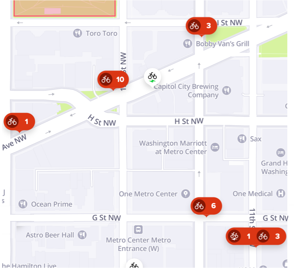
Figure 3: Locations of the Capital Bikeshare bike stations that are considered for our analysis.

We are motivated to apply our method to this dataset because of the dynamic nature of bike-sharing systems. The system allows customers to rent bikes from any bike-sharing station using an app and then return the bike to any bike-sharing station at their convenience. This flexibility requires the company managing the bike-sharing system to relocate bikes between stations in response to demand fluctuations. Accurately predicting this demand can greatly enhance the efficiency of these systems. Additionally, customers seeking to rent bikes tend to go towards nearby stations with available bikes, when one station has limited availability. Consequently, the demand for bikes at one station is closely intertwined with the demand at nearby stations, creating a high degree of correlation. Our approach accounts for these interdependencies to provide more effective predictions for optimizing bike-sharing operations.

As mentioned earlier, our response variables correspond to the demand for bikes at the five different bike stations across three time periods on a given day $(T)$, resulting in a total of $p=15$ responses. The covariates used in our experiment are the bike demand at these five stations during the same time periods over the last three days $(T-1,T-2,T-3),$ giving us $q=45$ covariates. Our goal is to get accurate predictions by leveraging the information we get from the conditional dependency structure between the responses and between the responses and the past demand.

We consider two different extents for this data. In the initial configuration, we have data for January 2023 $(n=31)$; in the second configuration, we have data from January - March 2023 $(n=90)$. We also create the training and testing set in two different ways. In the first setup, we split the data into train and test with 80% of the data belonging to the training set and 20% belonging to the test. In the next set of experiments, we maintain the 80% training set while distributing the remaining 20% from the test set differently. Here, we assume that half of the values in the test set are known and the other half are unknown. We solely predict the unknown values. These training and testing set-ups are demonstrated in figure 4. Comparing the two setups helps in evaluating the impact of incorporating the response dependencies (estimated via $\hat{\Lambda}$) into the predictions on the performance of the methods.

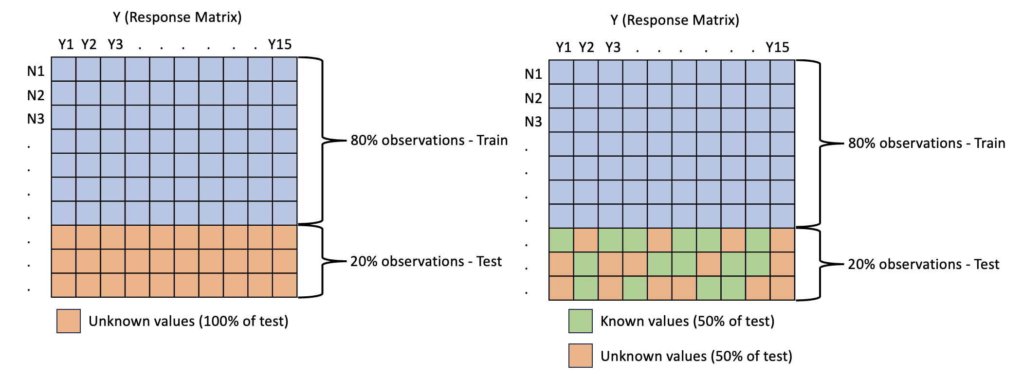
Figure 4: Two different training and testing setups. Left - Train and test with an 80 - 20 split. Right - Train and test with an 80 - 20 split, but half of the test responses are considered to be known.

We compare the prediction accuracy of our method against Graphical LASSO (or GLASSO), CAPME and Bayes CRF (or BCRF). The tuning parameters for each of these methods have been chosen from 5-fold cross-validation and the average prediction errors are evaluated by:

$$\bar{Err}=\frac{1}{n}\sum_{d=1}^{n}\|Y_{d}-\hat{Y_{d}}\|_{2},$$

where $d$ denotes a particular day.

The average prediction errors for all the methods are provided in Table 10. From the results, we can see that our method outperforms all the other methods consistently. Additionally, it is interesting to note that when the sample size ($n=31$) is less than the number of covariates ($p=45$), our method exhibits significantly better performance. Conversely, when the sample size is larger, Graphical LASSO and Bayes CRF have comparable performance. This is because our method uses the induced group sparsity to select only the relevant variables which is critical when the number of covariates is large.

It is also worth highlighting that the CAPME method performs poorly when confronted with scenarios where all test values are unknown. This is due to the omission of the second stage of CAPME in this setup, wherein it predicts response dependencies. Consequently, the full potential of CAPME remains untapped in this context. In contrast, when half of the test values are unknown, it leverages the value of $\Lambda$ to predict these unknown responses, showcasing a more comprehensive utilization of its capabilities. This is reflected in the lower magnitude of errors for the other methods as well.

	All test values unknown		Half test values unknown
Method	N = 31	N = 90	N = 31	N = 90
BVS.GM	18.734	22.222	10.439	12.483
GLASSO	25.657	22.687	16.832	16.907
BCRF	26.638	24.345	14.681	12.770
CAPME	53.160	108.424	39.895	23.269

Table 10: Average prediction error for capital bike-share demand

6 Conclusion

In the space of estimating the relationship within high dimensional responses and covariates, we introduce a Bayesian model designed to simultaneously estimate three distinct sparsity structures: the conditional dependency structure among the responses, the conditional dependency structure between the responses and the covariates, and the regression coefficient matrix. The proposed methodology bridges a significant gap in the literature on variable selection and sparse estimation for high-dimensional graphical models which currently focus either on the sparse estimation of the precision matrix or the regression coefficient matrix. Our empirical results demonstrate the capability of our method to be particularly useful when the signal strength is low.

References

- Bai et al., (2020) Bai, R., Ročková, V., and George, E. I. (2020). Spike-and-Slab Meets LASSO: A Review of the Spike-and-Slab LASSO. Handbook of Bayesian Variable Selection.
- Cai et al., (2013) Cai, T. T., Li, H., Liu, W., and Xie, J. (2013). Covariate-adjusted precision matrix estimation with an application in genetical genomics. Biometrika, 100(1):139–156.
- Candes and Tao, (2007) Candes, E. and Tao, T. (2007). The Dantzig selector: Statistical estimation when is much larger than . The Annals of Statistics, 35(6):2313–2351.
- Castillo et al., (2015) Castillo, I., Schmidt-Hieber, J., and van der Vaart, A. (2015). Bayesian linear regression with sparse priors. Annals of Statistics, 43(5):1986–2018.
- Consonni et al., (2017) Consonni, G., La Rocca, L., and Peluso, S. (2017). Objective Bayes covariate-adjusted sparse graphical model selection. Scandinavian Journal of Statistics, 44(3):741–764.
- Deshpande et al., (2019) Deshpande, S. K., Ročková, V., and George, E. I. (2019). Simultaneous variable and covariance selection with the multivariate spike-and-slab LASSO. Journal of Computational and Graphical Statistics, 28(4):921–931.
- Fan and Li, (2001) Fan, J. and Li, R. (2001). Variable selection via nonconcave penalized likelihood and its oracle properties. Journal of the American Statistical Association, 96(456):1348–1360.
- Friedman et al., (2008) Friedman, J., Hastie, T., and Tibshirani, R. (2008). Sparse inverse covariance estimation with the graphical LASSO. Biostatistics, 9(3):432–441.
- Gan et al., (2019) Gan, L., Narisetty, N. N., and Liang, F. (2019). Bayesian regularization for graphical models with unequal shrinkage. Journal of the American Statistical Association, 114(527):1218–1231.
- Gan et al., (2022) Gan, L., Narisetty, N. N., and Liang, F. (2022). Bayesian estimation of Gaussian conditional random fields. Statistica Sinica, 32:131–152.
- Honorio et al., (2012) Honorio, J., Samaras, D., Rish, I., and Cecchi, G. (2012). Variable selection for gaussian graphical models. In Artificial Intelligence and Statistics, pages 538–546. PMLR.
- Ishwaran and Rao, (2005) Ishwaran, H. and Rao, J. S. (2005). Spike and slab variable selection: frequentist and Bayesian strategies. The Annals of Statistics, 33(2):730–773.
- Lafferty et al., (2001) Lafferty, J., McCallum, A., and Pereira, F. C. (2001). Conditional random fields: Probabilistic models for segmenting and labeling sequence data. Machine Learning, 46(1-3):283–334.
- Li et al., (2022) Li, S., Cai, T. T., and Li, H. (2022). Transfer learning in large-scale gaussian graphical models with false discovery rate control. Journal of the American Statistical Association, pages 1–13.
- Li and McCormick, (2019) Li, Z. R. and McCormick, T. H. (2019). An expectation conditional maximization approach for Gaussian graphical models. Journal of Computational and Graphical Statistics, 28(4):767–777.
- Loh and Wainwright, (2013) Loh, P.-L. and Wainwright, M. J. (2013). Regularized M-estimators with nonconvexity: Statistical and algorithmic theory for local optima. Advances in Neural Information Processing Systems, 26.
- Mohammadi et al., (2023) Mohammadi, R., Massam, H., and Letac, G. (2023). Accelerating Bayesian structure learning in sparse Gaussian graphical models. Journal of the American Statistical Association, 118(542):1345–1358.
- Narisetty and He, (2014) Narisetty, N. N. and He, X. (2014). Bayesian variable selection with shrinking and diffusing priors. The Annals of Statistics, 42(2):789–817.
- Osborne et al., (2020) Osborne, N., Peterson, C. B., and Vannucci, M. (2020). Latent Network Estimation and Variable Selection for Compositional Data Via Variational EM. Journal of Computational and Graphical Statistics, 31:163 – 175.
- Radosavljevic et al., (2014) Radosavljevic, V., Vucetic, S., and Obradovic, Z. (2014). Neural gaussian conditional random fields. In Machine Learning and Knowledge Discovery in Databases: European Conference, ECML PKDD 2014, Nancy, France, September 15-19, 2014. Proceedings, Part II 14, pages 614–629. Springer.
- Ravikumar et al., (2011) Ravikumar, P., Wainwright, M. J., Raskutti, G., and Yu, B. (2011). High-dimensional covariance estimation by minimizing -penalized log-determinant divergence. Electronic Journal of Statistics, 5:935 – 980.
- Rigollet, (2015) Rigollet, P. (2015). High dimensional statistics lecture notes. https://ocw.mit.edu/courses/18-s997-high-dimensional-statistics-spring-2015/resources/mit18_s997s15_chapter2/.
- Ročková, (2018) Ročková, V. (2018). Bayesian estimation of sparse signals with a continuous spike-and-slab prior. The Annals of Statistics, page 401 – 437.
- Ročková and George, (2014) Ročková, V. and George, E. I. (2014). EMVS: The EM approach to Bayesian variable selection. Journal of the American Statistical Association, 109(506):828–846.
- Ročková and George, (2016) Ročková, V. and George, E. I. (2016). Fast Bayesian factor analysis via automatic rotations to sparsity. Journal of the American Statistical Association, 111(516):1608–1622.
- Ročková and George, (2018) Ročková, V. and George, E. I. (2018). The spike-and-slab LASSO. Journal of the American Statistical Association, 113(521):431–444.
- Rothman et al., (2010) Rothman, A. J., Levina, E., and Zhu, J. (2010). Sparse multivariate regression with covariance estimation. Journal of Computational and Graphical Statistics, 19(4):947–962.
- Sohn and Kim, (2012) Sohn, K.-A. and Kim, S. (2012). Joint estimation of structured sparsity and output structure in multiple-output regression via inverse-covariance regularization. In Artificial Intelligence and Statistics, pages 1081–1089. PMLR.
- Wytock and Kolter, (2013) Wytock, M. and Kolter, Z. (2013). Sparse Gaussian conditional random fields: Algorithms, theory, and application to energy forecasting. In International Conference on Machine Learning, pages 1265–1273. PMLR.
- Yang et al., (2021) Yang, X., Gan, L., Narisetty, N. N., and Liang, F. (2021). GemBag: Group estimation of multiple Bayesian graphical models. The Journal of Machine Learning Research, 22(1):2450–2497.
- Yin and Li, (2011) Yin, J. and Li, H. (2011). A sparse conditional Gaussian graphical model for analysis of genetical genomics data. The Annals of Applied Statistics, 5(4):2630.
- Yuan and Zhang, (2014) Yuan, X.-T. and Zhang, T. (2014). Partial Gaussian graphical model estimation. IEEE Transactions on Information Theory, 60(3):1673–1687.
- Zhang and Li, (2022) Zhang, J. and Li, Y. (2022). High-dimensional gaussian graphical regression models with covariates. Journal of the American Statistical Association, pages 1–13.