A Deep Learning Earth System Model for Stable and Efficient Simulation of the Current Climate

Abstract

A key challenge for computationally intensive state-of-the-art Earth-system models is to distinguish global warming signals from interannual variability. Recently machine learning models have performed better than state-of-the-art numerical weather prediction models for medium-range forecasting. Here we introduce DLESyM, a parsimonious deep learning model that accurately simulates the Earth’s current climate over 1000-year periods with negligible drift. DLESyM simulations equal or exceed key metrics of seasonal and interannual variability–such as tropical cyclone genesis and intensity, and mid-latitude blocking frequency–for historical simulations from four leading models from the 6th Climate Model Intercomparison Project. DLESyM, trained on both historical reanalysis data and satellite observations, is a key step toward an accurate highly efficient model of the coupled Earth system, empowering long-range sub-seasonal and seasonal forecasts.

1 Introduction

Enhanced Earth-system simulators are needed to better characterize critical thresholds and address the grand challenge of achieving global sustainability [1]. Accurate simulation of the Earth system to test hypotheses and evaluate sensitivities using state-of-the-art (SOTA) numerical Earth-system models requires enormous computational resources available only at large national and international centers. Coordinated experiments with these models through the Coupled Model Intercomparison Project (CMIP), have “become one of the foundational elements of climate science" [2]. To obtain dramatically more efficient and accessible simulations of the current climate, we introduce the Deep Learning Earth SYstem Model (DLESyM), a parsimonious machine-learning (ML) model whose fidelity to many aspects of the current climate system is comparable or even superior to several leading CMIP6 models.

ML models have recently demonstrated superiority over more traditional numerical weather prediction models for single deterministic global weather forecasts out to about 10 days [3, 4, 5, 6, 7]. Yet these same deterministic models become unstable or give unrealistic atmospheric states when iteratively rolled out for a full year [8]. One key for improving multi-year simulations is to correctly incorporate the sea surface temperature (SST). Simply specifying climatological sea surface temperatures (SST) as external forcing can improve the fidelity of some ML and ML-hybrid atmospheric models over decadal rollouts [9, 10]. Moving beyond externally specified SSTs, a reduced-complexity general circulation model (GCM) relying on conventional numerical methods has been coupled with a ML ocean model that predicts only SST to create 70-year simulations of the current climate [11]. As a first step with a fully ML coupled atmosphere-ocean model [12] were able to approximate oceanic signatures of El Niño and equatorial waves over 6-month forecast rollouts before instabilities developed.

Here we present our Deep Learning Earth SYstem Model (DLESyM) in a basic form that couples a parsimonious deep learning weather prediction model (DLWP) [8] with a deep learning ocean model (DLOM). We examine the performance and climatology of DLESyM over 100- and 1000-year iterative rollouts. Our model does not include anthropogenic forcing beyond what is incorporated in the training data, so our free-running simulations match the current climate.

A unique property of DLESyM is it’s ability to correctly simulate the current climate over a 1000-year iterative rollout with negligible drift. The empiricism associated with training our model on past reanalysis and observational data may be contrasted with the empirical tuning of model parameters required to minimize the drift in pre-industrial simulations with CMIP models. DLESyM captures extratropical interannual and synoptic-scale variability as well as or better than leading CMIP6 models with similar horizontal resolution (about 1^∘ in latitude). In the tropics, DLESyM’s climatology of spontaneously generated tropical cyclones and the Outgoing Longwave Radiation (OLR) signature of the Indian Summer Monsoon is superior to those of CMIP6 models. Despite being a autoregressive model with no generative components, DLESyM forecasts continue to generate sharply defined weather patterns over 1000 years (730,000 steps) into the rollout.

It is remarkable that such accurate behavior over long time scales is achieved through training our DLWP with a loss function that minimizes error over just 24 hours. The loss function for the DLOM minimizes errors over eight days, which is also short compared to the time scales over which SSTs evolve. The ability of the DLESyM to learn the current climate using such short-period training data sidesteps concerns about the lack of appropriate long-period datasets to train purpose-built ML models for seasonal and multi-year simulations [13].

As in SOTA CMIP6 Earth-system models, the coupling between the atmosphere and the ocean in DLESyM is asynchronous, with 6-hour time resolution in the atmosphere and 2-day resolution in the ocean. In comparison to the most successful medium-range ML forecast models [3, 4, 5, 6, 7], we adopt a much more parsimonious approach using an order of magnitude less prognostic variables at each grid point: 9 for the atmosphere and just SST for the ocean. Precipitation is not simulated directly as part of the autoregressive rollout, but rather diagnosed from the forecast fields with a separate deep learning module. Our training data includes fields from the ERA5 reanalysis, but in contrast to most previous models, we extend our set of prognostic fields to include outgoing long wave radiation (OLR) trained on observations from the International Satellite Cloud Climatology Project (ISCCP). Details about the architecture and training of DLESyM are presented in the Methods section.

2 1000-Year Simulation

The model’s accurate reproduction of the annual cycle and negligible drift is illustrated in Fig. 1a, which shows the first and last 5 years of a 1000-year (730,000-step) simulation initialized on January 1, 2017 along with the ERA5 verification for the period 2017-2022. Similar results generating the same average climate were obtained for 12 shorter 100-year simulations initialized on the first day of the month throughout a full year. The field contoured as a function of time and latitude in Fig. 1 is zonally averaged 500 hPa geopotential height ($Z_{500}$), which is high in the tropics and lowest in the wintertime pole. The same field is shown for the ERA5 reanalysis for the years 2017-2021 Fig. 1b. There is no predictability for the precise atmospheric state beyond roughly two weeks, but the climatological variations in the annual cycle of $Z_{500}$ are essentially identical in the reanalysis, the first 5 years, and the last five years of the 1000-year simulation.

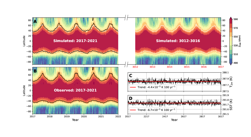
Figure 1: Zonally averaged 3-day mean of $Z_{500}$ plotted as a function of time and latitude: (A) for the first and last 5 years of a recursive 1,000-year model simulation initialized on 1 January 2017 (B) corresponding $Z_{500}$ field from the ERA5 reanalysis for the years 2017-2022. Also plotted are 15-day averaged values for the 560 dam contour for the DLESyM simulation (white line) in (A) and for ERA5 (black line) as a reference in both (A) and (B). Globally averaged annual mean (D) T_2m and (E) SST (black) during the 1,000 year simulation with the linear fit (red) and the trend noted in each panel.

Drift in global-mean values of the simulated fields is an important concern in climate modeling. Any drift must be sufficiently small that it does not mask actual changes from internal variability or anthropogenic forcing such as greenhouse-gas emissions. Drift can arise during spin-up as coupled models are initialized [14] and from nonclosure of global mass and energy budgets [14]. To reduce drift, conventional coupled GCMs must be spun up for centuries before beginning an actual experiment. The computational costs of long spin-ups can be prohibitive, so experiments often begin in states that are not fully equilibrated [15, 16].

Despite the DLESyM’s atmospheric and ocean modules being trained separately, there is no startup transient or spin-up period in the globally averaged 2-m air temperature and SST (Fig. 1d,e). The drifts in both surface air temperature and SST are two orders of magnitude smaller than that in pre-industrial scenarios in many CMIP models [16, 17]. It should be emphasized that these results are obtained without using training loss functions that constrain long-term drift; instead errors are simply minimized over periods of one day in the atmosphere and eight days in the ocean.

3 High Impact Cyclones

Extratropical cyclones (ETC) modulate the day-to-day cool-season weather through the passage of low and high pressure systems. A single severe ETC can cause catastrophic flooding, widespread power outages, and significant fatalities[18, 19]. Medium range ML weather forecast models have demonstrated skill in forecasting even severe ETCs at short lead times [20], but the features forecast by many of these models are excessively smoothed over longer lead times [4, 7]. Our DLESyM spontaneously generates realistic ETCs with sharply defined features throughout the full 1000-year rollout. For example, intense surface winds wrap around the 1000-hPa height ($Z_{1000}$) low center of a “Nor’easter" that develops near the end of the rollout in January 3016 just southeast of Newfoundland (Fig. 2e,f).

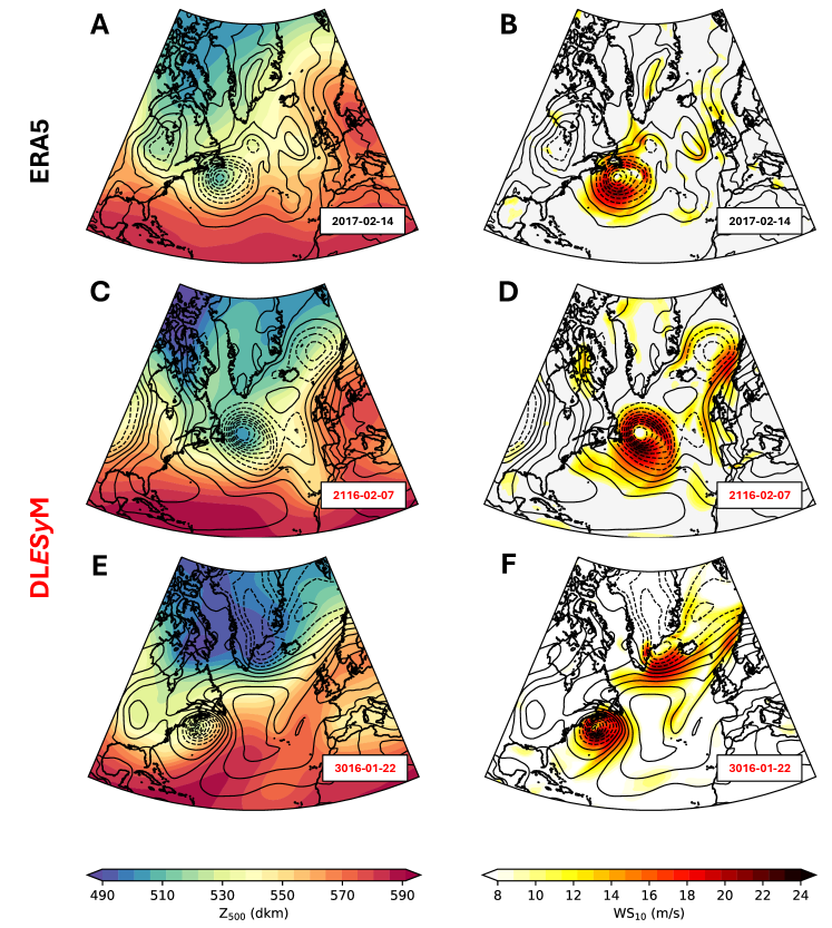
Figure 2: (A) Observed $Z_{1000}$, which is proportional to mean sea-level pressure (black contours, c.i.=4 dkm, contours $\leq 0$ dkm are dashed) and $Z_{500}$ (color fill) on February 14^th 2017. Data are plotted at 1^∘ latitude-longitude resolution. (B) As in (A), with color fill showing 10-m wind speed. (C), (D) as in (A), (B) for a simulated storm on February 7, 2116 in the 100th year of the DLESyM rollout. (E), (F) as in (C), (D) for January 22, 3016, in the 1000th year of the rollout.

For comparison, the same ERA5 fields for a roughly similar Nor’easter observed on February 14, 2017 are plotted in Fig. 2a,b. This observed storm is strong, but still a bit weaker in amplitude than the one in our 1000-year rollout. Another example of a Nor’easter traveling across the Atlantic in the 100th year of the rollout is shown in Fig. 2c,d. The upper-level $Z_{500}$ field in this case is notably similar to that observed on February 14, 2017.

Tropical cyclones (TCs) have been responsible for more fatalities than any other single weather event; the 1970 Bhola TC killed 250,000–500,000 people in Bangladesh [21]. The largest TC in the world are those in the Western North Pacific (WNP) [22], motivating us to compare the climatology of TC generation over the WNP during the last 30 years of a 100-year rollout from January 1, 2017 with 30 years of ERA5 data and historical simulations from four leading CMIP6 models.

An example of one of the top ten strongest spontaneously generated TCs near the end of the rollout (in August 2114) is compared with super typhoon Dale from the top ten TC in the ERA5 reanalysis (on November 12, 1996) in Fig. 3a,b. Both TC have the same amplitude in $Z_{1000}$, although the 10-m wind speeds are weaker in the DLESyM simulation, likely because of the relatively coarse 110-km grid spacing in our model.

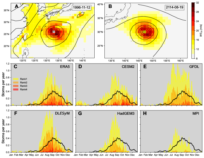
Figure 3: Tropical cyclone simulation and climatology in the WNP. (A) ERA5 reanalysis on November 12, 1996 and (B) DLESyM on August 19, 2114 showing $Z_{1000}$ (black contours, c.i.=6 dkm, contours $\leq 0$ dkm are dashed) and 10-m wind speeds (color fill). Both ERA5 and DLESyM fields are plotted at 1^∘ latitude-longitude resolution. (C)–(H): average frequency of TCs in storms per day from ERA5 and CMIP6 historical runs from 1985-2014, or 2085-2114 from DLESyM. Presence of a TC is determined from low sea-level pressure (CMIP6) or low $Z_{1000}$ (ERA5 and DLESyM) together with warm-core structure aloft (Methods 8.8). Black curve in (C)-(H) is the running 20-day average frequency of Rank 2 storms in ERA5.

Similar O(100) km grid spacing is also a serious limitation in CMIP6 models. Figure 3c-i compares the TC frequency in the WNP over the 30-year period 2085-2114 in the rollout with the period 1985-2014 in the ERA5 reanalysis and four historical CMIP6 runs. Except for the HadGEM3-GC31-LL, which use a 50% coarser mesh, the CMIP6 results were obtained using roughly the same grid spacing as DLESyM. All four CMIP6 models have difficulty capturing the correct frequency and intensity of TCs in the ERA5 reanalysis, particularly for more intense storms. The DLESyM generates a more accurate TC climatology than all models except perhaps CESM2. The peak in its annual cycle occurs roughly one month early compared to the ERA5 reanalysis, a shift likely produced by a similar one-month shift in the SSTs simulated in this region (Fig. 15). Recalling the simplicity of our DLOM, this shift might be reduced using a more complete ocean model.

4 Extra-tropical variability

High-amplitude ridges over western Europe are associated with both the simulated and observed Nor’easters, as apparent in the northward extension of the $Z_{500}$ field over Scandinavia (Fig. 2a,c,e). A strong stationary ridge steers atmospheric flows along extended north-south trajectories leading ETCs to detour around the region underneath the ridge [23, 24, 25]. Such “blocking" generates anomalous temperature and precipitation patterns that may include extreme cold-air outbreaks [26, 27], heat waves [28], droughts and floods [29, 30].

Correctly capturing subseasonal and seasonal variability requires Earth-system models to faithfully reproduce the frequency, spatial distribution, and amplitude of blocking events. This is a challenge for the CIMP6 models [31][32] and a good test of the climatology in the long rollouts of DLESyM. Here we compare the 40-year periods 2070-2110 from the 100-year DLESyM rollout starting on January 1, 2017 with ERA5 reanalysis and CMIP6 historical runs for the period 1970-2010.

The spatial distribution of the time-mean frequency of northern-hemisphere blocking events is evaluated using the absolute geopotential height index (AGP) [33] (Methods 8.5). DLESyM closely approximates the blocking frequencies computed from ERA5, except near the dateline, where blocks develop too frequently over the Chukchi Sea (Figs 4a,b). Equivalent plots for the historical runs from four leading CIMP6 models previously analyzed in connection with TCs are shown in Fig. 11. The distribution and amplitude of blocking frequency in the DLESyM rollout is roughly similar to that in the CMIP6-models. A quantitative comparison of the performance of all these models is provided by the Taylor diagram [34] (Methods 8.6) in Fig. 4c, from which one can assess differences in spatial correlation, standard deviation, and centered RMSE between each model and ERA5.

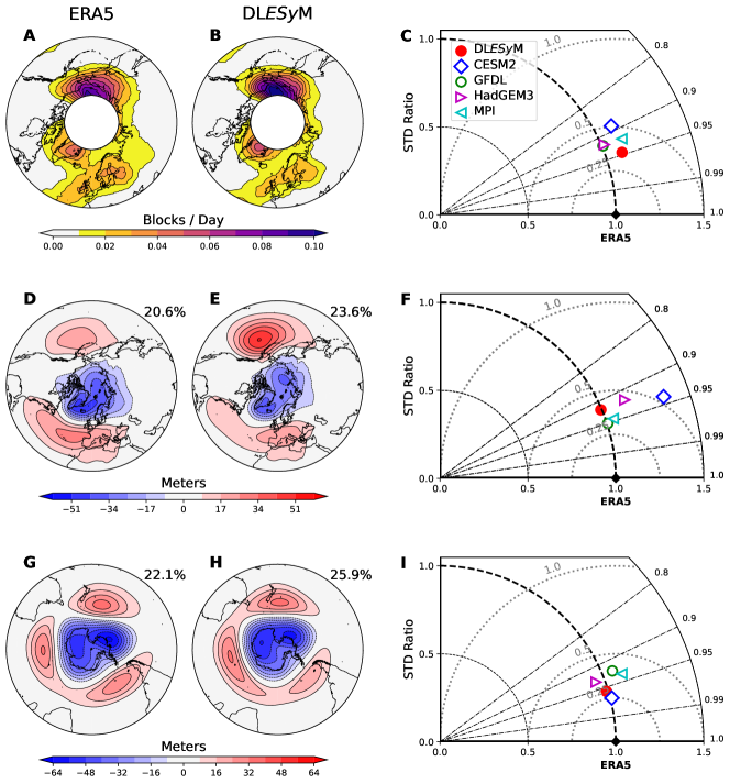
Figure 4: Mean frequency of northern hemisphere blocking during (A) the last 40 years of the 100-year DLESyM rollout and (B) from ERA5 (1970-2010). (C) Taylor diagram comparing blocking frequency for the same periods in DLESyM to that in ERA5 and to historical simulations (1970-2010) from selected CMIP6 models. EOFs associated with the NAM in (D) ERA5 and (E) DLESyM. Percentages give variance explained by each EOF. (F) Taylor diagram comparing the NAM in ERA5 with DLESyM, CESM2, GFDL-CM4, MPI-ESM1-2-HR and HadGEM3-GC31-LL. (G)–(I) as in (D)–(F) for the SAM.

DLESyM generates lower centered RMSE (having the least distance between the point plotted for each model and the point labeled ERA5 in Fig. 4c) and better spatial correlation than all four CMIP6 models. The normalized standard deviation for DLESyM is just slightly worse than for the MPI and CESM models, which are in turn, worse than the almost perfect standard deviation values for the GFDL and HadGEM models. Overall, the representation of blocking in the last 40 years of our 100-year rollout is at least as good as that in the historical runs from the compute-intensive SOTA CMIP6 models.

On longer time scales, the most important patterns extratropical hemispheric-scale variability are the Northern and Southern Annular Modes (the NAM and SAM). The NAM is the leading empirical orthogonal function (EOF) of the low-pass filtered $Z_{1000}$ field with the seasonal cycle removed; we similarly compute the SAM for the southern hemisphere using $Z_{500}$ (Methods 8.7). Geopotential height anomalies are low near the pole and high in mid-latitudes during the positive phase of the NAM and the SAM. High magnitudes of the NAM index are associated with statistically significant changes in the probability of impactful weather, including cold-air outbreaks and intense mid-latitude storms [35].

The fidelity of the DLESyM in reproducing the NAM over the last 40 years of our 100-year rollout is compared to that for year 1970–2010 in the ERA5 dataset in Fig. 4d,e. In both cases, the percentage of the variance explained, the spatial structure, and the amplitudes are very similar except over the North Pacific, where the signal is too strong in the DLESyM. As shown in Fig. 12, the comparable signal over the North Pacific is also too strong in three of the four CMIP6 historical simulations. The overall performance of the DLESyM and CMIP6 models are compared against the ERA5 NAM in the Taylor diagram in Fig. 4f. Both the GFDL and MPI models are superior to DLESyM, which in turn scores better than the other two CMIP6 models.

Turning to the southern hemisphere, the same set of comparisons is shown for the SAM in Fig. 4g–i and Fig. 13. The SAM analysis again demonstrates that DLESyM captures not just the correct climatology, but generates the correct low-frequency variance. As summarized in the Taylor diagram, DLESyM clearly outperforms three of the four CMIP6 models, only lagging behind CESM2.

5 Indian Summer Monsoon

The Indian summer monsoon (ISM) is a dominant feature in the annual cycle of tropical weather and has a crucial impact on agriculture. Increases or decreases of at least 10% in ISM rainfall have been associated with average deviations of $\pm 10$% in foodgrain production [36]. Here, we characterize the ISM by its signature in OLR, which can be directly compared with satellite observations. The 30-year mean annual cycle of the ISM index (after [37]; Methods: 8.9) over the period 1985-2014 in the ISCCP data closely matches that for years 2085-2114 in the 100-year DLESyM rollout through the start of November, after which the DLESyM’s ISM index increases more slowly (Fig. 5a).

The northward march of zonally averaged ISM convective cloud systems (low OLR) during onset, and their subsequent retreat to the south is illustrated for the same 30-year periods in Fig. 5b,c. The ISCCP data and the DLESyM again show very similar signatures except after November, south of 14^∘. Examination of the horizontal distribution of OLR within the ISM region late in the year indicates that the erroneously lingering deep convection in November and December lies over extreme southern India (Fig. 17). The four CMIP6 models also have difficulty accurately capturing the annual cycle of the ISM in their simulated OLR fields (Fig. 16). The superiority of DLESyM’s treatment of the seasonal cycle of zonally averaged OLR in the ISM, compared to the four CMIP6 models, is concisely illustrated by the Taylor diagram in Fig. 5d.

Turning from 30-year climatologies to a seasonal forecast, the OLR fields for a six-month DLESyM rollout beginning January 1, 2017 are compared against available ISCCP data within our testing split. The forecast for the ISM index closely follows ISCCP observations, however much of that signal is driven by climatology (Fig. 5a). Two-week averaged regional precipitation predicted at the end of the 6-month rollout is similar to the ERA5 verification (Fig. 5e,f). Further discussion of the forecast OLR and precipitation distributions during the 2017 monsoon onset appear in section 9.4.

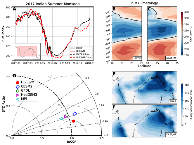
Figure 5: Indian Summer Monsoon (ISM) forecast and climatology in DLESyM. (A) Time series of forecasted 2017 ISM index (solid lines) and climatological index (dashed lines) for DLESyM (red) and ISCCP (black). The ISM index is the OLR averaged over the red box on the inserted map. (B) OLR Hovmoller of ISM climatology from 1985-2014 of the ISCCP record. (C) as in (B) calculated over years 2085-2114 of the DLESyM rollout. (D) Taylor diagram comparing spatio-temporal patterns displayed in (B), (C), and corresponding analyses from CMIP6 historical simulations. 14-day accumulated precipitation beginning June 12, 2017 for (E) ERA5 and (F) DLESyM 6-month forecast initialized January 1, 2017.

6 El Niño

The El Niño Southern Oscillation (ENSO) is the largest mode of interannual variability and can impact global weather patterns including precipitation over North America [38], the length of the South Asian Monsoon [39], the frequency and intensity of East Asian heatwaves [40] , and Antarctic [41] and Arctic sea ice variability [42]. DLESyM reproduces the characteristic temporal variations in the El Niño-Southern Oscillation (ENSO) though it underestimates its amplitude. Simulated teleconnections between ENSO phase and global SST and OLR closely match observed patterns of variability (Fig. 20). More in-depth discussion of ENSO variability in DLESyM appears in Section 9.5 of the Supplement. Further investigation of the oceanic response is left to future work.

7 Conclusion

Efforts to improve SOTA Earth-system models often focus on incorporating increasingly detailed representations of additional physical processes and extending to higher spatial resolutions. As a result, using these models becomes increasingly difficult for those without access to very high performance computing. Here we adopt a simpler and novel approach, asynchronously coupling a DLWP model with just 9 prognostic variables to a DLOM simulating SST, both using a 110-km globally-uniform mesh. The resulting DLESyM reproduces several aspects of the current climate at least as well as leading CMIP6 models at similar spatial resolution, yet as configured for this investigation, the DLESyM can complete a 1000-year simulation on a single NVIDIA A100 GPU in about 12 h. In contrast, running a 1000-year simulation with the National Center for Atmospheric Research’s CESM2.1.5 model at similar spatial resolution using 1280 processing elements on their SOTA HPE Cray EX, would take approximately 90 days.

The simulations shown here demonstrate that our DLESyM is not subject to several limitations that have been assumed to apply to the stability and accuracy of long autoregressive rollouts of deep learning Earth-system and weather forecast models [4, 43, 44]. In particular, the DLESyM simulation remains stable for 730,000 steps without significantly smoothing the structure of individual weather systems. Empiricism clearly underlies our data-driven machine learning approach, while playing a lesser role in traditional Earth-system models. CMIP models do, nevertheless, also include many empirically tuned parameters. For example, parameters are typically adjusted to minimize any drift in pre-industrial climate simulations remaining after an initial spin up period of several centuries. In contrast, there is no initial transience when our separately trained atmosphere and ocean models begin the coupled simulation, and the DLESyM’s drift in globally averaged 2-m air temperature and SST is two orders of magnitude smaller than that in many coupled CMIP6 models.

Surprisingly, the robust long-term properties of the DLESyM emerge after training it only on loss functions that focus on very short-term performance. Those loss functions consist of RMSE averaged over one day in the atmosphere and eight days in the ocean. No physical constraints or components of the training loss explicitly push the model toward the correct long-term behavior.

Climatologies of 30-y and 40-y periods from long iterative DLESyM rollouts were compared to similar length periods from the ERA5 reanalysis, ISCCP satellite observations, and historical runs from four CIMP6 models. The northern and southern annular modes (NAM and SAM) are captured with fidelity similar to the CMIP6 models as measured by spatial correlation, variance and RMSE. Because both the NAM and SAM are associated with extreme weather, long rollouts of DLESyM can help us understand extreme weather statistics

The frequency and spatial distribution of northern-hemisphere blocking is captured by DLESyM at least as well as by the CMIP6 models. In the tropics, DLESyM rollouts replicate the observed daily climatology of tropical cyclones in the western North Pacific and the Indian Summer monsoon better than the CMIP6 models.

Although it demonstrated success in this parsimonious configuration, there are clearly many avenues along which DLESyM can be improved. Perhaps the most obvious is to extend the DLOM beyond predicting just SST by adding fields characterizing the sea-surface height and upper-ocean heat content. Future work includes incorporating land-surface and sea-ice modules and testing configurations with additional atmospheric variables and finer spatial resolution.

One limitation of the DLESyM is that it is only applicable to simulations of the current climate. As such, the model is suitable for seasonal and sub-seasonal forecasting. Improvement of such long-timescale forecasts would be of enormous societal benefit, and ensemble DLESyM forecasts are being developed for this purpose. Forecasts of the future climate will require the model to incorporate forcing from greenhouse gases and anthropogenic aerosols; further investigation is warranted to determine whether this can be achieved by adding physical constraints to the model.

8 Materials and Methods

8.1 Model Design

DLESyM uses two U-net style convolutional neural nets [45] in autoregessive rollouts: one trained to simulate the atmosphere and the other, the ocean. The structures of these U-nets originate from a series of successful deep learning weather prediction models [46, 47, 8]. This section will focus on differences between the U-nets used in DLESyM and the architecture presented in [8], and on the coupling between the atmospheric and oceanic modules.

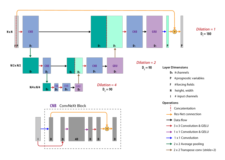
Figure 6: Schematic representation of the DLWP U-net as a sequence of operations on layers (see legend). U-net levels are labeled by their channel depth, with $D_{1}=180$ and $D_{2}=D_{3}=90$ being associated with the first convolutions in each level. Each ConvNeXt block (blue) is replaced by the layers and operations shown in the inset labeled CNB, with generic embedding depths $D$ and $I$ determined by the channel depth of the input and the labeled value of $D_{n}$. The purple blocks labeled GRU denote convolutional Gated Recurrent Unit layers, which are implemented with $1\times 1$ spatial convolutions. Other layers evaluated by the encoder are shown as dark green, while those evaluated by the decoder are shown as light green.

The structure of the atmospheric module is diagrammed in Fig. 6, with the details of the convolutional GRU [48] omitted for simplicity. Unlike the original ConvNeXt block proposed in [49], the ConvNeXt block in [8] expands the latent-layer depth by a factor of four as part of a spatial convolution with a $3\times 3$ kernel. Here we return to an architecture closer to that proposed in [49], where the expansion in latent-layer depth is imposed with a $1\times 1$ convolutional kernel. The resulting economy in the number of trainable weights allows us to substantially increase the latent-layer depth in each level of the U-net while reducing the total number of trainable parameters from 9.8M to 3.5M without loss of predictive skill.

The ocean module uses the same U-net architecture shown in Fig. 6, except layer depths at each level are reduced to $D_{1}=90$ and $D_{2}=D_{3}=45$, and the convolutional GRU is omitted to simplify the coupling algorithm. There are roughly 2.5M trainable parameters in the ocean module. Precipitation is diagnosed with a third U-net model. Like the ocean module, this model uses the architecture in Fig. 6 with the GRU’s omitted. The final output is the accumulated precipitation between the two model input times, rather than an updated model state. The layer depths are $D_{1}=64$, $D_{2}=128$, $D_{3}=256$, and the precipitation model uses roughly 1.5M trainable parameters.

8.2 Atmosphere-Ocean Coupling

The key challenge to forecast the ocean and atmosphere together is accommodating the different temporal resolution of the two models. Ocean circulations evolve more slowly than those in the atmosphere, so as in traditional Earth-system models, we use a longer time step for our ocean model. The DLOM updates every 4 days; each model step generates SST values at both 48-h and 96-h lead times. In contrast, the atmosphere updates every 12 hours, generating atmospheric fields at both 6-h and 12-h lead times. (See [8] for details about the two-in, two-out time stepping.)

To step the coupled model forward, we proceed in 96-h (4 day) increments. The mechanics of our coupling are illustrated in Figure 7. To describe the mechanism of our coupled model, we use $A$ to represent the atmospheric forecast and $S$ to represent the predicted oceanic forecast. The star operator, $\ast$, will indicate observed values. Subscripts are used to represent time, expressed in hours, relative to the initialization of the simulation with hour $0$ being the time at which the forecast is initialized.

The first step in our coupled simulations is to forecast the atmosphere. We use past and initial atmospheric states, $A^{\ast}_{-6}$, $A^{\ast}_{0}$ and the initial SST, $S^{\ast}_{0}$, to call the atmosphere model. This call produces predicted atmospheric states A₆ and A₁₂. Then, using these predicted atmospheric states and the same $S^{\ast}_{0}$, we call the atmospheric model again. This process is repeated, using the same SST, $S^{\ast}_{0}$, throughout, until we obtain a predicted atmosphere through 96 h. The ocean states S${}^{\ast}_{-48}$ and S${}^{\ast}_{0}$ are stepped forward using the $WS_{10}$, $Z_{1000}$ and OLR as forcing from the time-averaged atmosphere states $\overline{A_{48}}={\rm average}(A_{6},...,A_{48})$ and $\overline{A_{96}}={\rm average}(A_{54},...,A_{96})$ to produce the predicted ocean states S₄₈ and S₉₆. This completes a full 96-h cycle, which we repeat during iterative rollouts. Note that the 2-m atmospheric temperature is not passed to the ocean model in an effort to divorce causality from correlation, since the surface temperature over the ocean is primarily forced by the SST, not vice versa.

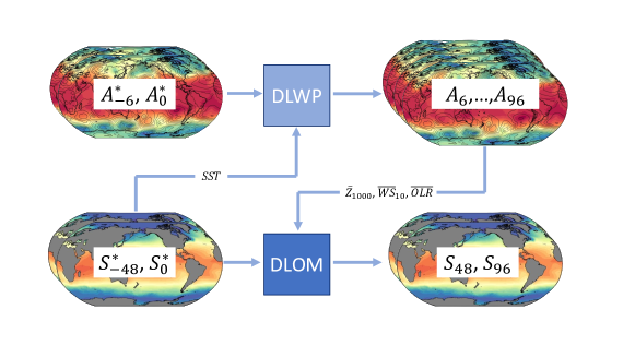
Figure 7: DLESyM coupling mechanism. Atmosphere and ocean states are denoted by $A$ and $S$, respectively, with the subscript indicating time in hours with respect to initialization at hour 0. Light blue box represents the atmospheric module (DLWP) while the darker blue represents the ocean (DLOM). Data flow and sequence of calls are given with arrows. For full description refer to section 8.2.

8.3 Data Sources

8.3.1 ERA5

ECMWF reanalysis version 5 (ERA5) [50] is the primary dataset used for training and verification of DLESyM providing these prognostic fields: geopotential at 1000, 700, 500, 300 and 250 hPa, temperature at 2-m and 850 hPa, total column water vapor, and SST. We also use two ERA5 time-invariant fields for training and inference: terrain height and land-sea fraction (called surface geopotential and land-sea mask in ERA5 database respectively.). Some of these fields require additional preprocessing using other ERA5 fields as indicated in Table 1.

As part of this reprocessing, SST data over the continents are imputed using zonal linear interpolation. This coast to coast interpolation ensures that our convolutional operations yield reasonable values throughout our domain while minimizing the sharp gradients near the land-sea boundaries. In addition to zonally interpolated imputation, we also tested the use of zonal climatological imputation. The later method, however, tended to produce nonphysical features in the ocean state during long rollouts. Although the full global SST is updated every step, the values over land are masked and ignored in the loss function during training.

ERA5 data and other data used in this study are summarized in Table 1. DLESyM discretizes all fields using the Hierarchical Equal Area isoLatitude Pixelization (HEALPix) [51, 8, 52], with the 12 tessellated HEALPix faces, each having $64\times 64$ grid points for a total of 49,152 points globally. The diagonal distance between adjacent nodes is approximately 110 km, which in turn is approximately 1°  of latitude at the equator.

8.3.2 ISCCP

The International Satellite Cloud Climatology Project (ISCCP) calibrates and compiles observations from a large suite of satellites into a single dataset [53]. For this study, we use the "IR Brightness Temperature" field from the HXG distribution, which is available from 1983 to 2017 at 3-hour resolution on a 0.1 degree latitude-longitude mesh. The ISCCP data requires several preprocessing steps before it is ready for training. There are swaths of missing data, notably prior to 1998 over the Indian Ocean, which are filled in using ERA5’s model-derived total net thermal radiation (TTR) field. To complete this imputation, IR brightness temperature is downsampled from the 0.1 degree latitude-longitude mesh to a 0.25°  mesh to match the ERA5 grid. Then TTR, in units of J m^-2, is scaled to match the distribution of the ISCCP brightness temperatures using the relation:

$$\widehat{\mbox{TTR}}=\frac{\sigma_{\mbox{IR}}}{\sigma_{\mbox{TTR}}}(\mbox{TTR}-\mu_{\mbox{TTR}})+\mu_{\mbox{IR}}$$ (1)

where $\widehat{\mbox{TTR}}$ is scaled TTR, $\sigma_{\rm IR}$ is the standard deviation of the IR brightness temperature, $\sigma_{\rm TTR}$ is the standard deviation of the TTR, $\mu_{\rm TTR}$ is the mean TTR, and $\mu_{\rm IR}$ is the mean IR brightness temperature. Once scaled, we use the TTR to impute the IR Brightness temperature over the missing regions of missing ISCCP data. A 2D Gaussian filter is used to smooth seams in the ISCCP observations and the imputed TTR. The result is a realistic OLR record that contains no missing data. Like ERA5 sourced data, ISCCP data was mapped onto the HEALPix mesh for training and inference.

Variable Name	Symbol	Source	Preprocessing
1000-hPa geopotential height	$Z_{1000}$	ERA5	-
500-hPa geopotential height	$Z_{500}$	ERA5	-
250-hPa geopotential height	$Z_{250}$	ERA5	-
700–300-hPa thickness	$\tau_{300-700}$	ERA5	difference between 300 and 700-hPa geopotential heights
2-m temperature	$T_{2m}$	ERA5	-
850-hPa temperature	$T_{850}$	ERA5	-
total column water vapor	TCWV	ERA5	-
10-m windspeed	$WS_{10}$	ERA5	magnitude of 10-m horizontal velocity vector
sea surface temperature	SST	ERA5	land imputation
outgoing longwave radiation	OLR	ISCCP	brightness conversion and OLR imputation
land-sea fraction	$F_{ls}$	ERA5	-
surface elevation	$z$	ERA5	-
top of atmosphere insolation	$I_{TOA}$	-	-

Table 1: Earth System fields ingested by DLESyM. The columns show the variable name, the abbreviated symbol for the variable, the data source, extra preprocessing steps used to prepare data for training/inference

8.4 Training the Deep Learning Earth System Model

While our ocean and atmosphere modules are coupled during inference (section 8.2), they are trained separately. We train each module to receive information about the other by using ERA5 and ISCCP data to initialize each training step. In this section we describe in detail the data, parameters, and curriculum used to train both the DLWP, DLOM, and the diagnostic precipitation module.

8.4.1 Deep Learning Weather Prediction Model

The DLWP training dataset is made up of four types of input: the 9 prognostic fields predicted by DLWP as well as 2 constant fields, 1 prescribed field, and 1 coupled field. Each of these inputs is interpreted by the neural net as a single channel. The constant fields are topographic height and land-sea fraction; the prescribed field is $I_{TOA}$ (which is calculated on-the-fly as a function of time, longitude, and latitude); the coupled field is SST. DLWP is trained on 33 years of observations (1983-2016) and validated on 1 year of observations (2016-2017).

As in [46], the atmosphere model is trained to optimize global root mean squared error (RMSE) over 24 hours, using data every 6-h generated by two model steps. Choosing a 24-h period for the loss allows the model to learn the atmospheric evolution in a complete diurnal cycle over the full globe without pushing it toward a multi-day ensemble mean forecast. Despite removing appropriate global mean values, and normalizing all the prognostic variables by their standard deviation, the contributions to the loss among individual variables differ by orders of magnitude; OLR and TCWV generate the largest losses, while $Z_{250}$ produces the smallest. We scale the weight for the $i^{\rm th}$ variable, $w_{i}$, to ensure the contributions to the RMSE loss function approximately balance the contributions from each field. Formally:

$$w_{i}=\frac{.001}{V_{i}},$$ (2)

where $V_{i}$ is the unscaled validation loss for the $i^{\rm th}$ variable after a 10-epoch training. We find that improvements achieved from weighting the loss function are not sensitive to the exact values of $w_{i}$.

Here we note important hyperparameter choices. This section is not comprehensive; the full model configuration will be published in the code repository associated with this article (Section  Data and Software Availability). Throughout training, we use the cosine annealing leaning rate scheduler as formulated by PyTorch’s optim library [54] over our 250 epoch training cycle. We used gradient clipping with max_norm=0.25. The DLWP model training took roughly 6.5 days on 4 NVIDIA A100 80GB graphics processing units (GPUs).

8.4.2 Deep Learning Ocean Model

Like DLWP, DLOM also has four basic types of input: prognostic, constant, prescribed, and coupled. SST is the single prognostic field predicted by our ocean component; DLOM receives $F_{LS}$ as a constant field; $I_{TOA}$ as a prescribed field; and $WS_{10m}$, $Z_{1000}$ and OLR from the atmosphere. The coupled fields used to force the training of the DLOM component have been averaged over times t₀-t₄₈ and t₄₈-t₉₆. This treatment of the incoming atmospheric fields is designed to mimic the behavior during inference (Section 8.2). Notably, we do not use $T_{2m}$ as a forcing field for DLOM, despite it being a prognostic field of our DLWP model. This is done to avoid SST values matching the $T_{2m}$ field above the ocean, when in fact it is the SST that should determine $T_{2m}$ over the ocean.

The DLOM component model is trained to optimize maritime RMSE over 192 h of prediction. Maritime RMSE is defined as the RMSE spatially weighted by $1-F_{LS}$. DLOM has 48-h resolution and so we advance 192 h from two auto-regressive calls (similar to the two calls in DLWP training).

We found that training DLOM models is more sensitive than training DLWP models. To achieve best results, we employed a staged learning program with 3 phases. The program proceeded for 300 epochs, with a restart every 100 epochs. The key difference between phases was the value of the learning rate. At the beginning of each phase the cosine annealing scheduler was reinitialized with different max and min values. Each phase began at the best performing model checkpoint from the previous phase and continued to a target epoch. A summary of the values used to initialize the cosine annealing learning rate scheduler in the 3 phases is given in Table 2. The DLOM model was trained over roughly 44 hours on 4 NVIDIA A100 80GB GPUs.

Phase	Max Epoch	Min LR	Max LR
1	100	4e-5	1e-4
2	200	5e-6	5e-5
3	300	0	2.5e-5

Table 2: Parameters used to initialize PyTorch cosine annealing learning rate scheduler at each phase of 3 phase staged learning. For full discussion of DLOM training routine, see Section 8.4.2.

8.4.3 Deep Learning Precipitation Diagnosis

The input to the diagnostic precipitation module is the same two-time-level tensor of prognostic, constant, and prescribed variables as DLWP, but rather than a recurrent forecast, its output $P$ is the cumulative 6-h precipitation between the two sequential times. The ERA5 precipitation over the same period is the target. Because precipitation is highly skewed, the loss function is evaluated as in [55] using the log-transformed field $\tilde{P}=\ln\left(1+P/\epsilon\right)$, where $\epsilon=1\times 10^{-8}$ m. To emphasize heavy precipitation events, the loss function is global RMSE of $\exp{(b*\tilde{P})}$, where $b=0.4$.

8.5 Evaluation of Atmospheric Blocking

The calculation of blocking in the DLESyM, CMIP6, and ERA5 fields uses the absolute geopotential index (AGP) as defined in [56]. AGP is a binary classification; a location in time and space is either experiencing blocking or not. To register as blocking, the 500-hPa geopotential height field at a specific point in the northern hemisphere at latitude $\phi_{0}$ must meet three criteria:

1. Reversal of the typical 500-hPa geopotential height gradient south of the location:

   $$\frac{Z_{500}(\phi_{0})-Z_{500}(\phi_{S})}{\phi_{0}-\phi_{S}}>0$$ (3)

   where $\phi_{S}$ is the latitude 15°  south of $\phi_{0}$.

2. Geostrophic wind is westerly north of the location:

   $$\frac{Z_{500}(\phi_{N})-Z_{500}(\phi_{0})}{\phi_{N}-\phi_{0}}<-10\,{\rm m\,({}^{\circ}\,latitude)}^{-1}$$ (4)

   where $\phi_{N}$ is 15°  north of $\phi_{0}$.

3. Persistence: the first two criteria must be satisfied for five consecutive days.

The code for assessing these three conditions was adapted from the repository published with [57]. The time-mean blocking frequency is evaluated pointwise throughout the domain and plotted in units of blocks per day.

8.6 Taylor diagram

Points are plotted on the Taylor diagram [34] in a cylindrical coordinate system. The radial distance at which a point is plotted is the ratio of the standard deviation of the field under evaluation to the standard deviation of the target field. The angle at which the point is plotted is given by the inverse cosine of the pattern correlation between the field under evaluation and the target. The target point is plotted on the abscissa at a radial distance of unity. This is the point where the target would appear if it were the field subjected to evaluation.

The centered pattern RMSE (see [34]) is given by the distance between the point for the field under evaluation and target point on the abscissa. This distance can be estimated by eye using the semi-circular dotted reference lines centered about the target point. Note that the radial line at angle $\theta$ is labeled by the argument of $\cos^{-1}(\theta)$, which is the pattern correlation.

8.7 Annular Mode Computation

The Northern Annular Mode (NAM), also commonly referred to as the Arctic Oscillation, is defined as the first Empirical Orthogonal Function (EOF) of the wintertime (November-April) monthly mean $Z_{1000}$ anomalies north of 20°N [58, 59]. The anomalies are first calculated by subtracting the climatology (seasonal cycle) at each latitude, longitude, and day of year, and then weighted by the square root of the cosine of latitude before determining the EOF. Daily values of NAM are obtained by projecting the daily anomalies onto the leading EOF patterns.

Since the majority of CMIP6 models have missing data in their $Z_{1000}$ fields, this study utilized sea-level pressure (SLP), a field not available in the DLESyM, to calculate the NAM for the CMIP6 models. The spatial correlation between the NAM computed from the $Z_{1000}$ and the SLP fields is 0.99, and, when plotted with properly calibrated contour intervals, their signatures are essentially identical, as shown in Figure. 8. Using these contour intervals for intercomparison in Figure 12, the NAM is plotted based on the $Z_{1000}$ field for ERA5 and the DLESyM rollout while the NAM is calculated from SLP for the CMIP6 historical runs. To maximize compatibility, the statistics for the NAM calculated from CMIP6 data are compared against the ERA5 SLP record in the Taylor diagram in Fig. 4.

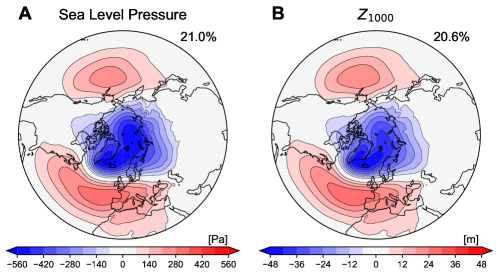
Figure 8: Leading mode of NH variability in ERA5 evaluated using (A) SLP and (B) $Z_{1000}$. Calculated over 40 years of ERA5 record (1970-2010). Contour intervals in Pa and m, as labeled, to reveal the same pattern.

The southern Annular Mode (SAM) calculation is nearly the same as NAM but for year-round monthly mean $Z_{500}$ anomalies south of 20°S. $Z_{500}$ is used instead of $Z_{1000}$ to avoid reduction-to-sea-level errors over the high terrain in Antarctica. The correlation between the NAM (SAM) index in this paper and the corresponding Arctic Oscillation (Antarctic Oscillation) daily time series provided by the Climate Prediction Center (CPC; https://www.cpc.ncep.noaa.gov/) for 1970–2010 (1979-2010) is 0.98 (0.93).

8.8 Determining Tropical Cyclone Frequency

The identification of potential tropical cyclones is based on the presence of a local minimum in SLP and an upper-level warm core, as outlined in [60, 61]. This research categorizes tropical cyclones into four groups based on these three criteria:

1. The local minimum in SLP drops below predefined thresholds within a specified area. In this study, these thresholds were established as round numbers approximating the 1st, 0.1st, 0.01st, and 0.001st percentile SLP values in the western North Pacific region (100°E–160°E, 5°N–35°N), specifically and 1000, 994, 985, 975 hPa for for fields sampled once per day.

2. The presence of a well-defined upper-level warm core. The warm core is defined as the geopotential layer thickness between 300 and 700 hPa that exceeds its climatological values.

3. The tropical cyclone trajectories are continuous. The adjacent centers along the same track are separated by no more than 2 days in time and 3 degrees in spatial distance. Tracks containing fewer than 3 data points are not considered in the analysis.

The DLESyM employed $Z_{1000}$ to identify tropical cyclones because it does not include SLP in its state vector. Both variables are available in ERA5, which allows us to calibrate the $Z_{1000}$ values in the DLESyM rollout for comparison with the CMIP6 historical runs. The difference between using SLP and $Z_{1000}$ for detecting tropical cyclones, with appropriately scaled thresholds, was negligible in this study. Choosing 0, -50, -130, -230 m as the $Z_{1000}$ thresholds corresponding to those previously noted for SLP, we obtain the comparison tropical cyclone frequencies shown in 9. The correlations between the distributions for Ranks 1 to 4 is 0.99, 0.99, 0.98, and 0.89, respectively.

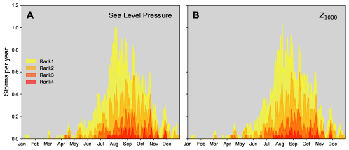
Figure 9: Comparison of TC detection algorithm applied to ERA5 using (A) SLP and (B) $Z_{1000}$. Nearly identical structure of TC frequency justifies comparisons between DLESyM simulations (which only predict $Z_{1000}$) and CMIP6 output (which only reports SLP).

8.9 Indian Summer Monsoon

Analyses reporting the Indian Summer Monsoon or ISM follow metrics defined in [37]. Outgoing longwave radiation values are spatially averaged between 10°  and 25°  North and 70°  and 100°  East to obtain the ISM index. Plotted time series in Figure 5a are daily average values of this ISM Index.

9 Supplementary Text

9.1 Global precipitation climatology

We diagnose precipitation with a DL architecture similar to that used in the ocean model (8.1). Fig. 10 shows that the annual averaged precipitation from the last 41 years of our 100-year rollout closely matches ERA5 precipitation for the years 1979-2020, including in regions of heavy precipitation. An exception is in the equatorial Pacific, where the DLESyM gives an over-estimate. Unlike the ISCCP OLR, the ERA5 precipitation is almost exclusively model generated, and therefore subject to error. The actual precipitation is difficult to observe, although analyses such as Integrated Multi-satellitE Retrievals for GPM (IMERG) are available. Detailed comparisons between DLESyM and observed precipitation are left for further study.

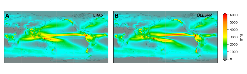
Figure 10: Climatology of global annual precipitation from (A) ERA5 reanalysis for 1979-2020, (B) last 41 years of our 100-year rollout.

9.2 Mid-latitude variability

Mid-latitude variability is characterized in Fig. 4 by comparing blocking and the annular modes in DLESyM for the last 40 years of the 100-year January 1, 2017 rollout and ERA5 reanalysis for the period 1970-2010. Also compared in that same figure are the blocking frequency, the NAM, and the SAM from the period 1970-2010 from historical runs of four CMIP6 models through concise Taylor diagrams. To augment the Taylor-diagram analysis, hemispheric plots comparing the structure of these signals in the CMIP6 simulations to that in ERA5 and the DLESyM are shown in Figs. 11–13. The CMIP6 models used for these historical runs are the CESM2, GFDL-CM4, HadGEM3-GC31-LL and MPI-ESM1-2-HR.

DLESyM blocking frequency over the Atlantic sector appears to be better than those from all four of the CMIP6 simulations; on the other hand, DLESyM gives the greatest overestimation of blocking in the western Arctic Ocean (Fig. 11). Slightly farther south, the tendency of the models to over-estimate the amplitude of the NAM in the north Pacific region is present in all simulations except the GFDL run, and it is worse in the CESM2 and HadGEM3 than in the DLESyM (Fig. 12). Turning to the SAM, the overall pattern, and the Taylor diagram scores, are both better for the DLESyM than for three of the four CMIP6 models (Fig. 13). The SAM in the CESM2 historical runs is, however, slightly better than that in the DLESyM rollout.

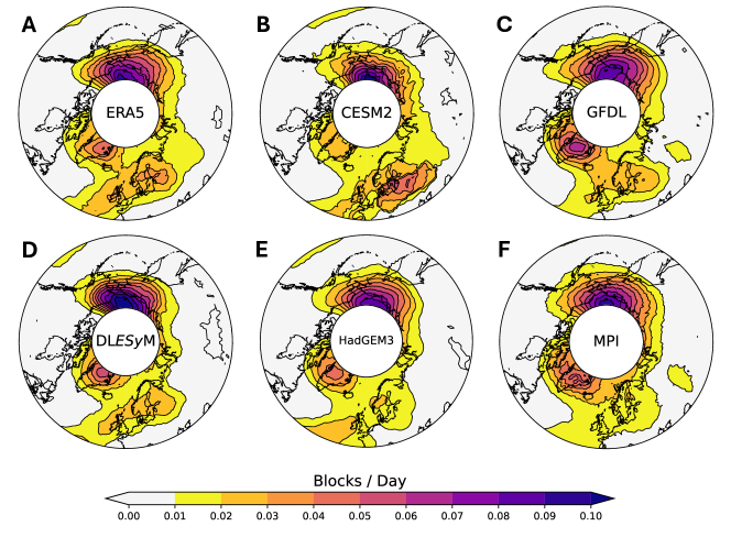
Figure 11: Blocking frequency in ERA5, DLESyM, and CMIP6. (A) annual NH blocking frequency 40 years of the ERA5 record (1970-2010). (B, C, E, F) as in (A) computed over historical CMIP6 simulations, source models labelled in of polar projection. (D) annual NH blocking frequency in the last 40 years of 100 year DLESyM rollout.

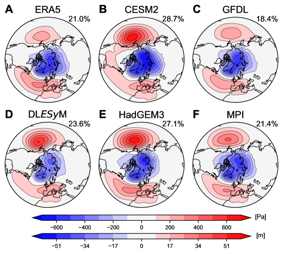
Figure 12: Leading mode of NH variability in (A) ERA5 $Z_{1000}$ during 1970-2010; (B) SLP simulated by CESM2 for CMIP6 historical experiment; (C, E, F) as in (B) except using GFDL-CM4, HadGEM3-GC31-LL, and MPI-ESM1-2-HR respectively. (D) shows same analysis as (A) evaluated over the last 40 years of the 100 year DLESyM rollout.

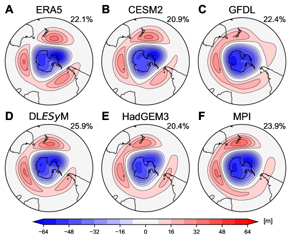
Figure 13: Leading mode of NH $Z_{500}$ variability in (A) ERA5 during 1970-2010; (B) simulated by CESM2 for CMIP6 historical experiment; (C, E, F) as in (B) except using GFDL-CM4, HadGEM3-GC31-LL, and MPI-ESM1-2-HR respectively. (D) shows same analysis as (A) evaluated over the last 40 years of the 100 year DLESyM rollout.

9.3 Tropical Cyclones

As illustrated in Figure 3c,f, the seasonal distribution and frequency of spontaneously generated western North Pacific tropical cyclones over the last 30 years in our 100-year January 1, 2017 rollout is similar to that in the ERA5 data over the 30-year period 1985-2014. To further characterize these cyclones, tracks are plotted for each storm over the 5-year periods 2010-2014 in ERA5 and 2110-2114 in the DLESyM rollout (Fig. 14).

These tracks use data at 6-h time resolution, with ranks 1–4 representing storms that, at their highest intensity, again exceed thresholds corresponding to approximately the 1st, 0.1st, 0.01st, and 0.001st percentile $Z_{1000}$ values in warm core systems over the western North Pacific region. Because the 6-h sampling increases the dataset size relative to once-a-day sampling, these ranks correspond to deeper geopotential-height thresholds of -10, -100, -200, and -300 m. The simulated cyclones follow similar tracks to those in the ERA5 reanalysis and show a similar distribution, except that strong TC are over represented in the eastern part, and under represented in the central part, of the domain in the DLESyM rollout.

As also apparent when comparing the climatologies in Figure 3c,f, the maximum TC frequency peaks about one month too early in the DLESyM rollout. This early peak is likely produced by a similar one-month early peak in the SSTs as shown by the annual cycle of their averages over the North Pacific region (100°E–160°E, 5°N–35°N) in Figure 15. These values are also averaged over the same 30-year period used for the TC analysis in both datasets. While there is a shift in the peaks and valleys of the distribution, the SSTs in the DLESyM rollout do closely follow the correct climatology, never deviating by more than 0.3^∘ K.

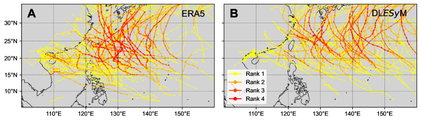
Figure 14: Tropical cyclone tracks in western North Pacific over a 5-year period from (A) ERA5 (2010-2014), (B) from the DLESyM rollout (2110–2114).

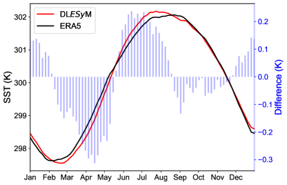
Figure 15: Annual variation in area-averaged SST values in NW Pacific from ERA5 (black) and the DLESyM (red). Vertical bars indicate the difference between the two averaged SST values.

9.4 Indian summer monsoon

The annual north-south cycle in OLR over south Asia is illustrated in Fig. 5 for 30-years of ISCCP data over the period 1985-2014 and for the DLESyM rollout for 2085-2114. The performance of the OLR simulated by the CMIP6 models during historical runs for 2085-2114 is also compared with the DLESyM result and the ISCCP observations in a Taylor diagram in Figure 5. The Hovmoller diagrams for longitudinally average observed and forecast OLR, which are evaluated in the Taylor diagram, are plotted in Figure 16. Like the DLESyM, all the CMIP6 models have difficulty properly capturing the southward progression of the low OLR signal in November and December. As indicated by the Taylor diagram in Figure 5, the best overall reproduction of the ISCCP climatology is generated in the DLESyM rollout.

The 30-year climatology of the full horizontal structure of the OLR field in the south Asian monsoon region, averaged over 2- or 3-month periods in the annual cycle, is shown (Fig. 17) for the ISCCP observations and DLESyM rollout. During monsoon onset (May–July) and the beginning of it southward retreat (September–October), the DLESyM fields are in close agreement with the observations. In the November–December period, however, the OLR values are too low over southern India and the adjacent Indian Ocean, which leads to the errors at low-latitudes apparent in November and December in Figure 16a,d.

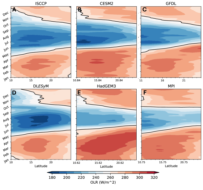
Figure 16: Climatology of the north-south progression of the annual cycle of OLR in Indian Summer Monsoon region. Hovmoller diagrams of the longitudinally averaged OLR in (A) the ISCCP data, and computed from the (B) CESM2, (C) GFDL-CM4, (D) DLESyM, (E) HADGEM3-GC31 and (F) MPI-ESM1-2-HR.

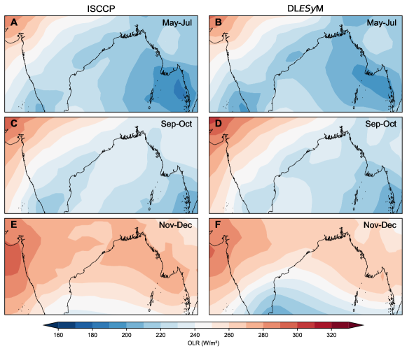
Figure 17: Climatology of the annual cycle of multi-month averaged of OLR in (A), (C), (E) ISCCP data for 1985-2014, and (B), (D), (F) years 2085-2114 in the DLESyM rollout. Averaging period is indicated in each panel.

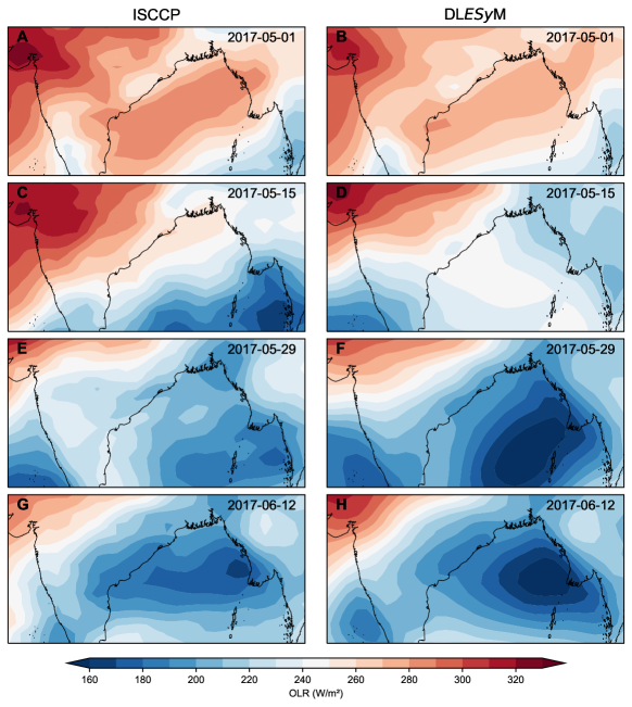
Figure 18: May–June 2017 progression of 2-week-averaged OLR for the period beginning on the date noted in each panel in (A), (C), (E), (G): ISCCP data, and (B), (D), (F), (H): 6-month DLESyM forecast from January 1, 2017.

A more detailed comparison of DLESyM treatment of monsoon onset during May and June in a 6-month forecast beginning on January 1, 2017 is presented by 2-week averaged fields of OLR (Fig. 18) and 2-week accumulated precipitation (Fig. 19). The OLR is observed by satellite, while the ERA5 precipitation in this region is generated by the ECMWF’s global forecast model during each reanalysis cycle. Considering the six-month forecast lead time, the predicted and analyzed fields are in reasonably good agreement in three of the four 2-week periods, with substantial differences only during May 15-28.

Some of this good agreement is facilitated by the strong climatological forcing for the Indian Summer Monsoon. The extent to which DLESyM can correctly capture interannual variations in monsoon onset in ensemble forecasts is a subject of current research. Nevertheless, Figs. 18) and 19 demonstrate that key atmospheric fields simulated by DLESyM at the end of the 6-month rollout are physically realistic.

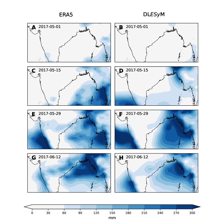
Figure 19: May–June 2017 progression of 2-week accumulated precipitation fields for the period beginning on the date noted in each panel in (A), (C), (E), (G): ERA5, and (B), (D), (F), (H): 6-month DLESyM forecast from January 1, 2017.

9.5 El Niño Southern Oscillation

The El Niño Southern Oscillation (ENSO) is the largest mode of interannual variability and can impact remote regions of the globe via atmospheric teleconnections. ENSO has a center of action in the equatorial Pacific. El Niño, the positive (warm) phase of ENSO, is characterized by a weak west-east equatorial Pacific SST gradient, weak trade winds, and deep convection in the central and eastern equatorial Pacific. In contrast, La Niña, the negative (cold) phase of ENSO, is associated with strong trade winds, an enhanced west-east equatorial Pacific SST gradient, and strong deep convection in the western equatorial Pacific. ENSO is predominately driven by coupled interactions between the atmosphere and ocean in the tropical Pacific[62, 63], and readers are referred to [64] for a full review of ENSO dynamics.

Given the importance of ENSO for global interannual variability, we examine the performance of DLESyM in simulating a realistic ENSO. Our DLESyM spontaneously generates variability in the Niño 3.4 (5N-5S, 170W-120W; black box) region comparable to observations, albeit weaker in magnitude (Fig. 20a). There is no tendency for the model to drift toward a warm or cold state in the equatorial Pacific. Instead, weak El Niños or La Niñas with magnitudes of the Niño 3.4 index exceeding 0.5 develop with a period of roughly 4 years, consistent with observations. In order to examine patterns of variability, SST and OLR anomalies for observations Figure 20(b-c) and model output Figure 20(d-e) are regressed onto their respective standardized Niño 3.4 (5N-5S, 170W-120W; black box) times series. Remarkably, maps of these regression coefficients, interpreted as the SST and OLR anomalies associated with a positive one standard-deviation Niño 3.4 anomaly, reveal that our DLESyM generates patterns of variability consistent with observations. Associated with an El Niño (i.e. a positive one standard-deviation Niño 3.4 anomaly) DLESyM exhibits widespread warming and cooling in the east and west Pacific, respectively, and a weakening of the climatological west-east equatorial SST gradient. Coincident with this pattern of SST changes is a decrease in OLR in the central Pacific, suggestive of deep convection, high cloud-tops, and a shift in the Walker circulation, and an increase in OLR in the west and east Pacific, characteristic of subsidence and reduced cloud cover. Moreover, the similarity between the DLESyM and observed response pattern of SSTs and OLR in remote ocean basins (i.e. Atlantic and Southern Oceans) suggests the our DLESyM may capture the remote atmospheric teleconnections associated with ENSO.

Despite the amplitude bias in DLESyM’s ENSO, these results strongly suggest that, with modest improvements, this DLESyM may be a powerful new tool for studying ENSO variability. Recall that the ocean module in our DLESyM is quite basic, predicting only SST. A more complete model capable of capturing atmosphere-ocean interactions, thermal damping, and upper-ocean dynamics would likely be able to better capture realistic ENSO amplitudes.

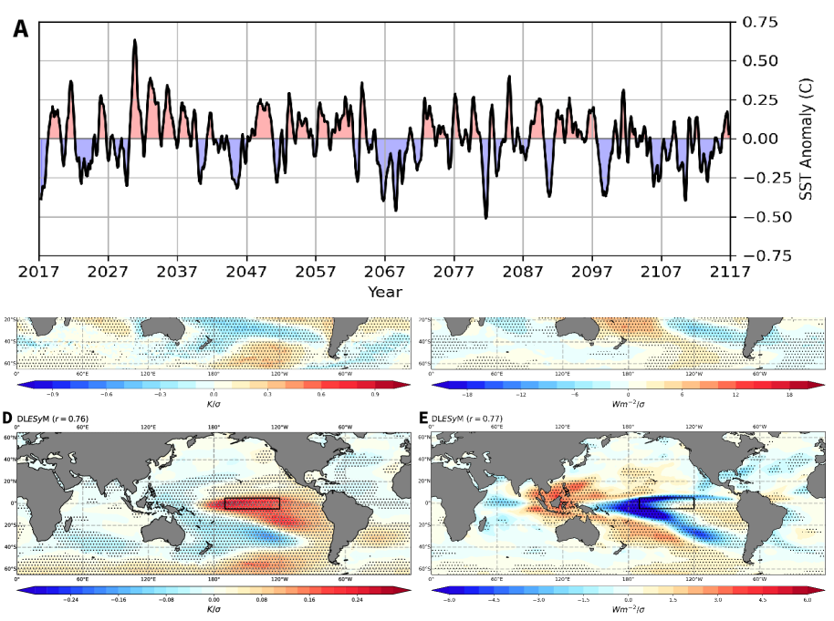
Figure 20: (A) Niño 3.4 index (5N-5S, 170W-120W; black box) computed from the perturbation of the equatorial SSTs from the monthly climatology in the 100-year January 1, 2017 rollout . Anomally patterns of (B) ERA5 SST, (C) ISCCP OLR, (D) DLESyM SST, and (E) DLESyM OLR regressed onto their respective standardized Niño 3.4 times series. Stippling indicates statistical significance (p $\leq$ 0.05) computed from a 2-tailed p-value associated with Pearson correlation coefficient.

Data and Software Availability

All data used within this study has been obtained through publicly available data repositories. ERA5 data was downloaded from ECMWF’s Climate Data Store [50, 65]. ISCCP data is made available by NOAA’s National Center for Environmental Information (NCEI) initiative [66]. Code required for data preparation, model training/inference, and analysis will be published on github (https://github.com/AtmosSci-DLESM/DLESyM). CMIP6 data was downloaded using the acccmip6 open source project (acccmip6.readthedocs.io).

Author Contributions

DLESyM Conceptualization: DRD, NCC. Software development: NCC, MK. DLESyM training: NCC. Precipitation module conceptualization: DRD and RM. Precipitation module training: RM. DLESyM Execution of rollouts: NCC. Data curation: NCC, MK, BL, RM. Analysis design: DRD, NCC, BL, ZE. Analysis execution: BL, NCC, ZE, RM. Writing - main text: DRD. Writing – materials and methods: NCC, DRD, BL, RM. Writing – supplement: DRD, ZE, RM. Writing – revisions: NCC, DRD, ZE, MK, BL, RM. Figures: BL, NCC, RM, ZE, DRD. Project coordination: DRD.

References

- [1] W. V. Reid, D. Chen, L. Goldfarb, H. Hackmann, Y. T. Lee, K. Mokhele, E. Ostrom, K. Raivio, J. Rockström, H. J. Schellnhuber, and A. Whyte. Earth system science for global sustainability: Grand challenges. Science, 330(6006):916–917, 2010.
- [2] Veronika Eyring, Sandrine Bony, Gerald A. Meehl, Catherine A. Senior, Bjorn Stevens, Ronald J. Stouffer, and Karl E. Taylor. Overview of the Coupled Model Intercomparison Project Phase 6 (CMIP6) experimental design and organization. Geoscientific Model Development, 9(5):1937–1958, 2016.
- [3] Kaifeng Bi, Lingxi Xie, Hengheng Zhang, Xin Chen, Xiaotao Gu, and Qi Tian. Accurate medium-range global weather forecasting with 3D neural networks. Nature, 619(7970):533–538, 2023.
- [4] Remi Lam, Alvaro Sanchez-Gonzalez, Matthew Willson, Peter Wirnsberger, Meire Fortunato, Ferran Alet, Suman Ravuri, Timo Ewalds, Zach Eaton-Rosen, Weihua Hu, Alexander Merose, Stephan Hoyer, George Holland, Oriol Vinyals, Jacklynn Stott, Alexander Pritzel, Shakir Mohamed, and Peter Battaglia. Learning skillful medium-range global weather forecasting. Science, 382(6677):1416–1421, 2023.
- [5] Kang Chen, Tao Han, Junchao Gong, Lei Bai, Fenghua Ling, Jing-Jia Luo, Xi Chen, Leiming Ma, Tianning Zhang, Rui Su, Yuanzheng Ci, Bin Li, Xiaokang Yang, and Wanli Ouyang. FengWu: Pushing the Skillful Global Medium-range Weather Forecast beyond 10 Days Lead. arXiv:2304.02948, 2023.
- [6] Lei Chen, Xiaohui Zhong, Feng Zhang, Yuan Cheng, Yinghui Xu, Yuan Qi, and Hao Li. FuXi: A cascade machine learning forecasting system for 15-day global weather forecast. npj Climate and Atmospheric Science, 6(1):1–11, 2023.
- [7] Simon Lang, Mihai Alexe, Matthew Chantry, Jesper Dramsch, Florian Pinault, Baudouin Raoult, Mariana C. A. Clare, Christian Lessig, Michael Maier-Gerber, Linus Magnusson, Zied Ben Bouallègue, Ana Prieto Nemesio, Peter D. Dueben, Andrew Brown, Florian Pappenberger, and Florence Rabier. AIFS - ECMWF’s data-driven forecasting system. arXiv:2406.01465, 2024.
- [8] Matthias Karlbauer, Nathaniel Cresswell-Clay, Dale R. Durran, Raul A. Moreno, Thorsten Kurth, Boris Bonev, Noah Brenowitz, and Martin V. Butz. Advancing Parsimonious Deep Learning Weather Prediction Using the HEALPix Mesh. Journal of Advances in Modeling Earth Systems, 16(8):e2023MS004021, 2024.
- [9] Oliver Watt-Meyer, Gideon Dresdner, Jeremy McGibbon, Spencer K. Clark, Brian Henn, James Duncan, Noah D. Brenowitz, Karthik Kashinath, Michael S. Pritchard, Boris Bonev, Matthew E. Peters, and Christopher S. Bretherton. ACE: A fast, skillful learned global atmospheric model for climate prediction, 2023. arXiv:2310.02074.
- [10] Dmitrii Kochkov, Janni Yuval, Ian Langmore, Peter Norgaard, Jamie Smith, Griffin Mooers, James Lottes, Stephan Rasp, Peter Düben, Milan Klöwer, Sam Hatfield, Peter Battaglia, Alvaro Sanchez-Gonzalez, Matthew Willson, Michael P. Brenner, and Stephan Hoyer. Neural General Circulation Models, 2023. arXiv:2311.07222 [physics].
- [11] Troy Arcomano, Istvan Szunyogh, Alexander Wikner, Brian R. Hunt, and Edward Ott. A hybrid atmospheric model incorporating machine learning can capture dynamical processes not captured by its physics-based component. Geophysical Research Letters, 50(8):e2022GL102649, 2023.
- [12] Chenggong Wang, Michael S. Pritchard, Noah Brenowitz, Yair Cohen, Boris Bonev, Thorsten Kurth, Dale Durran, and Jaideep Pathak. Coupled ocean-atmosphere dynamics in a machine learning earth system model. arXiv:2406.08632, 2024.
- [13] Catherine O. de Burgh-Day and Tennessee Leeuwenburg. Machine learning for numerical weather and climate modelling: A review. Geoscientific Model Development, 16(22):6433–6477, November 2023.
- [14] Stefan Rahmstorf. Climate drift in an ocean model coupled to a simple, perfectly matched atmosphere. Climate Dynamics, 11(8):447–458, 1995.
- [15] A. Yool, J. Palmiéri, C. G. Jones, A. A. Sellar, L. de Mora, T. Kuhlbrodt, E. E. Popova, J. P. Mulcahy, A. Wiltshire, S. T. Rumbold, M. Stringer, R. S. R. Hill, Y. Tang, J. Walton, A. Blaker, A. J. G. Nurser, A. C. Coward, J. Hirschi, S. Woodward, D. I. Kelley, R. Ellis, and S. Rumbold-Jones. Spin-up of UK Earth System Model 1 (UKESM1) for CMIP6. Journal of Advances in Modeling Earth Systems, 12(8):e2019MS001933, 2020.
- [16] Alexander Sen Gupta, Nicolas C. Jourdain, Jaclyn N. Brown, and Didier Monselesan. Climate Drift in the CMIP5 Models. Journal of Climate, 2013.
- [17] J. K. Ridley, E. W. Blockley, and G. S. Jones. A Change in Climate State During a Pre-Industrial Simulation of the CMIP6 Model HadGEM3 Driven by Deep Ocean Drift. Geophysical Research Letters, 49(6):e2021GL097171, 2022.
- [18] Mattha Busby, Miranda Bryant, Lili Bayer, Mattha Busby (now); Miranda Bryant, and Lili Bayer (earlier). Storm Ciarán: deaths reported across Europe while UK faces major disruption – as it happpened. the Guardian, 2023.
- [19] Jon Henley and Jon Henley Europe correspondent. Storm Ciarán: Seven people killed and dozens injured in Europe. The Guardian, 2023.
- [20] Andrew J. Charlton-Perez, Helen F. Dacre, Simon Driscoll, Suzanne L. Gray, Ben Harvey, Natalie J. Harvey, Kieran M. R. Hunt, Robert W. Lee, Ranjini Swaminathan, Remy Vandaele, and Ambrogio Volonté. Do AI models produce better weather forecasts than physics-based models? A quantitative evaluation case study of Storm Ciarán. npj Climate and Atmospheric Science, 7(1):1–11, 2024.
- [21] Naomi Hossain. The 1970 Bhola cyclone, nationalist politics, and the subsistence crisis contract in Bangladesh. Disasters, 42(1):187–203, 2018.
- [22] Kelvin T. F. Chan and Johnny C. L. Chan. Global climatology of tropical cyclone size as inferred from QuikSCAT data. International Journal of Climatology, 35(15):4843–4848, 2015.
- [23] Daniel F. Rex. Blocking Action in the Middle Troposphere and its Effect upon Regional Climate. Tellus, 2(4):275–301, 1950.
- [24] Tim Woollings. Dynamical influences on European climate: an uncertain future. Philosophical Transactions: Mathematical, Physical and Engineering Sciences, 368(1924):3733–3756, 2010.
- [25] Anthony R. Lupo. Atmospheric blocking events: a review. Annals of the New York Academy of Sciences, 1504:5–24, 2021.
- [26] J. Cattiaux, R. Vautard, C. Cassou, P. Yiou, V. Masson-Delmotte, and F. Codron. Winter 2010 in Europe: A cold extreme in a warming climate. Geophysical Research Letters, 37(20), 2010.
- [27] Kirien Whan, Francis Zwiers, and Jana Sillmann. The Influence of Atmospheric Blocking on Extreme Winter Minimum Temperatures in North America. Journal of Climate, 29(12):4361–4381, June 2016.
- [28] David Barriopedro, Erich M. Fischer, Jürg Luterbacher, Ricardo M. Trigo, and Ricardo García-Herrera. The Hot Summer of 2010: Redrawing the Temperature Record Map of Europe. Science, 332(6026):220–224, 2011.
- [29] Peter Bissolli, Karsten Friedrich, Jörg Rapp, and Markus Ziese. Flooding in eastern central Europe in May 2010 – reasons, evolution and climatological assessment. Weather, 66(6):147–153, 2011.
- [30] R. A. Houze, K. L. Rasmussen, S. Medina, S. R. Brodzik, and U. Romatschke. Anomalous Atmospheric Events Leading to the Summer 2010 Floods in Pakistan. Bulletin of the American Meteorological Society, 92(3):291–298, 2011.
- [31] Reinhard Schiemann, Marie-Estelle Demory, Len C. Shaffrey, Jane Strachan, Pier Luigi Vidale, Matthew S. Mizielinski, Malcolm J. Roberts, Mio Matsueda, Michael F. Wehner, and Thomas Jung. The Resolution Sensitivity of Northern Hemisphere Blocking in Four 25-km Atmospheric Global Circulation Models. Journal of Climate, 30(1):337–358, 2017.
- [32] Paolo Davini and Fabio D’Andrea. From CMIP3 to CMIP6: Northern Hemisphere Atmospheric Blocking Simulation in Present and Future Climate. Journal of Climate, 33(23):10021–10038, December 2020.
- [33] Stefano Tibaldi and Franco Molteni. On the operational predictability of blocking. Tellus A, 42(3):343–365, 1990.
- [34] Karl E. Taylor. Summarizing multiple aspects of model performance in a single diagram. Journal of Geophysical Research: Atmospheres, 106(D7):7183–7192, April 2001.
- [35] David W. J. Thompson and John M. Wallace. Regional Climate Impacts of the Northern Hemisphere Annular Mode. Science, 293(5527):85–89, 2001.
- [36] B. Parthasarathy, A. A. Munot, and D. R. Kothawale. Regression model for estimation of Indian foodgrain production from summer monsoon rainfall. Agricultural and Forest Meteorology, 42(2):167–182, March 1988.
- [37] Bin Wang and Zhen Fan. Choice of South Asian Summer Monsoon Indices. Bulletin of the American Meteorological Society, 80(4):629–638, April 1999.
- [38] Chester F Ropelewski and Michael S Halpert. North american precipitation and temperature patterns associated with the el niño/southern oscillation (enso). Monthly Weather Review, 114(12):2352–2362, 1986.
- [39] Bhupendra Nath Goswami and Prince K Xavier. Enso control on the south asian monsoon through the length of the rainy season. Geophysical Research Letters, 32(18), 2005.
- [40] Ming Luo and Ngar-Cheung Lau. Amplifying effect of enso on heat waves in china. Climate Dynamics, 52(5):3277–3289, 2019.
- [41] Xiaojun Yuan. Enso-related impacts on antarctic sea ice: a synthesis of phenomenon and mechanisms. Antarctic Science, 16(4):415–425, 2004.
- [42] Robin Clancy, Cecilia Bitz, and Ed Blanchard-Wrigglesworth. The influence of enso on arctic sea ice in large ensembles and observations. Journal of Climate, 34(24):9585–9604, 2021.
- [43] Ilan Price, Alvaro Sanchez-Gonzalez, Ferran Alet, Timo Ewalds, Andrew El-Kadi, Jacklynn Stott, Shakir Mohamed, Peter Battaglia, Remi Lam, and Matthew Willson. GenCast: Diffusion-based ensemble forecasting for medium-range weather. arXiv:2312.15796v2, 2024.
- [44] Ashesh Chattopadhyay and Pedram Hassanzadeh. Long-term instabilities of deep learning-based digital twins of the climate system: The cause and a solution. arXiv:2304.07029, 2023.
- [45] Olaf Ronneberger, Philipp Fischer, and Thomas Brox. U-net: Convolutional networks for biomedical image segmentation. In Medical image computing and computer-assisted intervention–MICCAI 2015: 18th international conference, Munich, Germany, October 5-9, 2015, proceedings, part III 18, pages 234–241. Springer, 2015.
- [46] Jonathan A. Weyn, Dale R. Durran, and Rich Caruana. Improving Data-Driven Global Weather Prediction Using Deep Convolutional Neural Networks on a Cubed Sphere. Journal of Advances in Modeling Earth Systems, 12(9):e2020MS002109, 2020.
- [47] Jonathan A. Weyn, Dale R. Durran, Rich Caruana, and Nathaniel Cresswell-Clay. Sub-Seasonal Forecasting With a Large Ensemble of Deep-Learning Weather Prediction Models. Journal of Advances in Modeling Earth Systems, 13(7):e2021MS002502, 2021.
- [48] Nicolas Ballas, Li Yao, Chris Pal, and Aaron Courville. Delving deeper into convolutional networks for learning video representations. arXiv preprint arXiv:1511.06432, 2015.
- [49] Zhuang Liu, Hanzi Mao, Chao-Yuan Wu, Christoph Feichtenhofer, Trevor Darrell, and Saining Xie. A ConvNet for the 2020s, 2022. arXiv:2201.03545.
- [50] Hans Hersbach, Bill Bell, Paul Berrisford, Shoji Hirahara, András Horányi, Joaquín Muñoz-Sabater, Julien Nicolas, Carole Peubey, Raluca Radu, Dinand Schepers, Adrian Simmons, Cornel Soci, Saleh Abdalla, Xavier Abellan, Gianpaolo Balsamo, Peter Bechtold, Gionata Biavati, Jean Bidlot, Massimo Bonavita, Giovanna De Chiara, Per Dahlgren, Dick Dee, Michail Diamantakis, Rossana Dragani, Johannes Flemming, Richard Forbes, Manuel Fuentes, Alan Geer, Leo Haimberger, Sean Healy, Robin J. Hogan, Elías Hólm, Marta Janisková, Sarah Keeley, Patrick Laloyaux, Philippe Lopez, Cristina Lupu, Gabor Radnoti, Patricia de Rosnay, Iryna Rozum, Freja Vamborg, Sebastien Villaume, and Jean-Noël Thépaut. The ERA5 global reanalysis. Quarterly Journal of the Royal Meteorological Society, 146(730):1999–2049, 2020.
- [51] K. M. Górski, E. Hivon, A. J. Banday, B. D. Wandelt, F. K. Hansen, M. Reinecke, and M. Bartelmann. HEALPix: A Framework for High-Resolution Discretization and Fast Analysis of Data Distributed on the Sphere. The Astrophysical Journal, 622(2):759, 2005.
- [52] Andrea Zonca, Leo P. Singer, Daniel Lenz, Martin Reinecke, Cyrille Rosset, Eric Hivon, and Krzysztof M. Gorski. healpy: equal area pixelization and spherical harmonics transforms for data on the sphere in Python. Journal of Open Source Software, 4(35):1298, 2019.
- [53] Alisa H. Young, Kenneth R. Knapp, Anand Inamdar, William Hankins, and William B. Rossow. The International Satellite Cloud Climatology Project H-Series climate data record product. Earth System Science Data, 10(1):583–593, 2018.
- [54] Adam Paszke, Sam Gross, Francisco Massa, Adam Lerer, James Bradbury, Gregory Chanan, Trevor Killeen, Zeming Lin, Natalia Gimelshein, Luca Antiga, Alban Desmaison, Andreas Kopf, Edward Yang, Zachary DeVito, Martin Raison, Alykhan Tejani, Sasank Chilamkurthy, Benoit Steiner, Lu Fang, Junjie Bai, and Soumith Chintala. Pytorch: An imperative style, high-performance deep learning library. In H. Wallach, H. Larochelle, A. Beygelzimer, F. d'Alché-Buc, E. Fox, and R. Garnett, editors, Advances in Neural Information Processing Systems 32, pages 8024–8035. Curran Associates, Inc., 2019.
- [55] Stephan Rasp and Nils Thuerey. Data-driven medium-range weather prediction with a resnet pretrained on climate simulations: A new model for weatherbench. Journal of Advances in Modeling Earth Systems, 13(2), 2021.
- [56] Reinhard Schiemann, Panos Athanasiadis, David Barriopedro, Francisco Doblas-Reyes, Katja Lohmann, Malcolm J. Roberts, Dmitry V. Sein, Christopher D. Roberts, Laurent Terray, and Pier Luigi Vidale. Northern Hemisphere blocking simulation in current climate models: evaluating progress from the Climate Model Intercomparison Project Phase 5 to 6 and sensitivity to resolution. Weather and Climate Dynamics, 1(1):277–292, 2020.
- [57] Lukas Brunner and Andrea K. Steiner. A global perspective on atmospheric blocking using GPS radio occultation – one decade of observations. Atmospheric Measurement Techniques, 10(12):4727–4745, 2017.
- [58] David W. J. Thompson and John M. Wallace. The Arctic oscillation signature in the wintertime geopotential height and temperature fields. Geophysical Research Letters, 25(9):1297–1300, 1998.
- [59] Mark P. Baldwin and Timothy J. Dunkerton. Stratospheric Harbingers of Anomalous Weather Regimes. Science, 294(5542):581–584, 2001.
- [60] Paul A Ullrich, Colin M Zarzycki, Elizabeth E McClenny, Marielle C Pinheiro, Alyssa M Stansfield, and Kevin A Reed. Tempestextremes v2. 1: A community framework for feature detection, tracking, and analysis in large datasets. Geoscientific Model Development, 14(8):5023–5048, 2021.
- [61] Colin M Zarzycki and Paul A Ullrich. Assessing sensitivities in algorithmic detection of tropical cyclones in climate data. Geophysical Research Letters, 44(2):1141–1149, 2017.
- [62] Goratz Beobide-Arsuaga, Tobias Bayr, Annika Reintges, and Mojib Latif. Uncertainty of enso-amplitude projections in cmip5 and cmip6 models. Climate Dynamics, 56:3875–3888, 2021.
- [63] Jakob Bjerknes. Atmospheric teleconnections from the equatorial pacific. Monthly weather review, 97(3):163–172, 1969.
- [64] Chunzai Wang, Clara Deser, Jin-Yi Yu, Pedro DiNezio, and Amy Clement. El niño and southern oscillation (enso): a review. Coral reefs of the eastern tropical Pacific: Persistence and loss in a dynamic environment, pages 85–106, 2017.
- [65] Copernicus Climate Change Service. ERA5 hourly data on single levels from 1940 to present, 2018.
- [66] National Centers for Environmental Information (NCEI). International Satellite Cloud Climatology Project (ISCCP)-H Series, 2021.